We include uncertainties due to missing higher order corrections to QCD computations (MHOU) used in the determination of parton distributions (PDFs) in the recent NNPDF4.0 set of PDFs. We use our previously published methodology, based on the treatment of MHOUs and their full correlations through a theory covariance matrix determined by scale variation, now fully incorporated in the new NNPDF theory pipeline. We assess the impact of the inclusion of MHOUs on the NNPDF4.0 central values and uncertainties, and specifically show that they lead to improved consistency of the PDF determination with an ensuing moderate reduction of PDF uncertainties at NNLO.

1 Introduction

The uncertainty on the parton distribution functions (PDFs) that enter any prediction of physical processes is one main bottleneck for precision physics at the LHC. Thanks to methodological progress, especially the use of machine learning techniques and the increase of experimental information, we have recently achieved a determination of PDFs, NNPDF4.0 [1], whose nominal precision reaches the percent level. It is clearly crucial to assess whether this level of precision is reliable, and whether it is matched by the same level of accuracy.

A considerable effort has gone into assessing the impact on uncertainties of the methodology used for the determination of PDFs, and specifically the way it propagates the information contained in the data onto the PDF uncertainty (see e.g. the recent studies in Refs. [2, 3]). However, PDF uncertainties, as given in all standard PDF sets, such as NNPDF4.0 [1], CT18 [4], MSHT20 [5] or ABMP16 [6], do not include theoretical uncertainties, i.e., the uncertainties that affect the predictions that are compared to the data in the process of determining PDFs from a set of experimental data. The only exceptions are the parametric uncertainty related to the value of the strong coupling $\alpha_{s}$, which is routinely included since the early days of LHC physics [7], and nuclear uncertainties that affect e.g. deep-inelastic scattering (DIS) data on nuclear targets (such as neutrino DIS data), that are for instance included in the NNPDF4.0 PDF determination [8, 9].

In principle, theoretical uncertainties may come from a variety of different sources, both parametric (such as the values of the heavy quark masses) and non-parametric (such as the aforementioned nuclear corrections). Theory uncertainties related to missing higher orders in QCD computations — MHOUs henceforth — are particularly relevant, because they affect any prediction. The current typical perturbative accuracy of QCD computations is next-to-next-to-leading order (NNLO), with N³LO corrections only known in a small number of cases [10]. At NNLO, MHOUs are typically of the order of a few percent or bigger. For LHC precision observables used for PDF determination, such as gauge boson or top-pair production, this is surely comparable to the experimental systematic uncertainties, and often larger or even much larger than the experimental statistical uncertainty. Since the uncertainty on the experimental measurement and on the theoretical prediction enter in a completely symmetric way in the figure of merit used for PDF determination [2], there is no justification to include the former and not the latter if they are of comparable sizes.

In Refs. [11, 12] we have presented a methodology for the systematic inclusion of theory uncertainties in PDF fits through a theory covariance matrix, and for the computation of the theory covariance matrix related to MHOU through correlated scale variations. A first application of this methodology to the construction of a set of NLO PDFs with MHOUs, based on the NNPDF3.1 [13] PDF set and methodology, was also presented in these references, but no global NNLO PDF set with inclusion of MHOUs is currently available. Such a construction is now greatly facilitated by the availability of the EKO [14] evolution code, and its inclusion in a new pipeline for producing theory predictions for PDF determination [15], recently used for the construction of the NNPDF4.0QED PDF set [16] and currently adopted by NNPDF as a standard. Other approaches to the determination of MHOUs have been proposed [17, 18, 19, 20, 21, 22]; also, MHOUs on NNLO PDFs have been recently estimated based on an approximate N³LO PDF determination [23].

It is the purpose of this paper to include MHOUs in the NNPDF4.0 NLO and NNLO sets of parton distributions using the methdology of Refs. [11, 12]. The final deliverables of the paper are thus new versions of the NNPDF4.0 global PDF determination, with more accurate central values and uncertainties that now also account for the inclusion of MHOUs in the process of PDF determination. It was indeed shown in Refs. [11, 12] that the main effect of including MHOUs in PDF determination is to modify central values, specifically leading to better perturbative convergence. Parton distributions with MHOUs included in the PDF uncertainty should henceforth become the default choice.

This paper is organized as follows. First, in Section 2 we succinctly review the formalism of Refs. [11, 12] for the determination of a covariance matrix accounting for MHOUs and its implementation in a PDF fit, specifically referring to its recent implementation in the EKO evolution code. In Section 3 we present the MHOU covariance matrices at NLO and NNLO and validate the NLO covariance matrix by comparing the estimated MHOUs against the known NNLO results. The main deliverables of this paper, namely the NNPDF4.0 NLO and NNLO PDFs with MHOUs, are presented in Section 4, where they are compared, both in terms of central values and uncertainties, to their counterparts without MHOUs, thereby assessing the impact of MHOUs on the consistency of the PDF determination. Finally, in Section 5 we discuss the delivery and usage of the PDFs with MHOUs and summarize our results. In an Appendix we provide explicit expressions for the missing higher order terms that are generated upon performing renormalization and factorization scale variation, and that are used in Section 2 to construct the MHOU covariance matrix.

2 The MHOU covariance matrix

The inclusion of MHOUs is done by supplementing theory predictions with a covariance matrix that accounts for their expected correlated variation upon inclusion of higher-order corrections. This in turn is estimated through scale variation. The whole construction is explained in detail in Refs. [11, 12], to which we refer for a detailed discussion. In this section we provide a brief summary of the main aspects of the procedure, with specific reference to its implementation in the EKO [14] code that, as mentioned, is part of the new NNPDF theory pipeline [15] used in this paper. In particular, for ease of reference, in this Section we adopt the same notation as in the EKO documentation, even though they depart somewhat from those of Ref. [14].

We first summarize the way perturbative expansions of various quantities are defined; we then review the way MHOUs on hard cross sections and anomalous dimensions can be estimated by mean of scale variation, and we finally summarize the construction of the MHOU covariance matrix. The expressions that are needed for scale variation up to N³LO are summarized in Appendix A.

2.1 Perturbative expansion and factorization

We start by writing down explicitly the perturbative expansion of an observable factorized in terms of a hard cross-section and PDFs, with the main goal of establishing notation. Given this, we only consider the case of inclusive electroproduction with a single parton species. The hadronic observable is then a structure function $F(Q^{2})$ that depends on a physical scale $Q^{2}$, and it is written in terms of a partonic quantity, the coefficient function $C(Q^{2})$, perturbatively computed as an expansion in the strong coupling

$$a_{s}(Q^{2})\equiv\frac{\alpha_{s}(Q^{2})}{4\pi}$$ (2.1)

and a PDF $f(Q^{2})$. In Mellin space we simply have

$$F(Q^{2})=C(Q^{2})f(Q^{2}).$$ (2.2)

The partonic coefficient function (for hadronic processes the partonic cross-section) is expanded perturbatively, and at N^kLO it is given by

$$C\left(a_{s}(Q^{2})\right)=a_{s}^{m}(Q^{2})\sum_{j=0}^{k}\left(a_{s}(Q^{2})\right)^{j}C_{j}$$ (2.3)

where the LO cross-section is ${\cal O}(a_{s}^{m})$: so for deep-inelastic structure functions $m=0$ (in the case of $F_{2},F_{3}$) or $m=1$ (in the case of $F_{L}$), for top pair production $m=2$ and so on.

The scale dependence of the strong coupling $a_{s}(Q^{2})$ and of the PDF $f(Q^{2})$ are given by

$$\mu^{2}\frac{{\rm d}a_{s}(\mu^{2})}{{\rm d}\mu^{2}} =\beta(a_{s}(\mu^{2}))=-\sum_{j=0}^{k}\left(a_{s}(\mu^{2})\right)^{2+j}\beta_{j},$$ (2.4)

$$\mu^{2}\frac{{\rm d}f(\mu^{2})}{{\rm d}\mu^{2}} =-\gamma\left(a_{s}(\mu^{2})\right).f(\mu^{2})$$ (2.5)

At N^kLO the beta function and anomalous dimensions are respectively given by

$$\beta(a_{s}(\mu^{2})) =-\sum_{j=0}^{k}\left(a_{s}(\mu^{2})\right)^{2+j}\beta_{j},$$ (2.6)

$$\gamma\left(a_{s}(\mu^{2})\right) =\sum_{j=0}^{k}\left(a_{s}(\mu^{2})\right)^{1+j}\gamma_{j}.$$ (2.7)

The coefficients $\beta_{j}$ are known up to $k=4$ (N⁴LO or five loops) [24, 25, 26, 27], while the coefficients $\gamma_{j}$ are known exactly up to $k=2$ and approximately for $k=3$ (N³LO or four loops) [28, 29, 30, 31, 32, 33, 34, 23, 35]. The perturbative expansion of the solutions to Eqs. 2.4 and 2.5, which are needed in order to compute the scale variation terms that we are interested in, are given explicitly in Appendix A.

The solution to Eq. 2.5 can be written in the form of an evolution kernel operator (EKO) $E(\mu^{2}\leftarrow\mu_{0}^{2})$ [14] given by

$$f(\mu^{2})=E(\mu^{2}\leftarrow\mu_{0}^{2})f(\mu_{0}^{2})=\mathcal{P}\exp\left(-\int_{\mu_{0}^{2}}^{\mu^{2}}\frac{{\rm d}{\mu^{\prime}}^{2}}{{\mu^{\prime}}^{2}}\,\gamma\left(a_{s}({\mu^{\prime}}^{2})\right)\right)f(\mu_{0}^{2}),$$ (2.8)

where $\mathcal{P}$ denotes path ordering. Of course, including the anomalous dimension to N^kLO accuracy yields a PDF $f(Q^{2})$ whose scale dependence has a resummed (next-to-)^k-leading-logarithmic (N^kLL) accuracy. The perturbative expansion of this solution is given up to (fixed, i.e. not resummed) order $a_{s}^{3}$ in Appendix A.

2.2 MHOUs from scale variation

Theoretical predictions at hadron colliders depend on two quantities that are computed perturbatively: the partonic cross sections or coefficient functions, Eq. (2.3), and the anomalous dimensions, Eq. (2.7), that determine the scale dependence, Eq. (2.8), of the PDF. Both quantities can be expressed as a series in the strong coupling $a_{s}(Q^{2})$, in turn perturbatively given, through the solution to Eq. (2.4), in terms of the value of the strong coupling at a reference scale, typically $a_{s}(M_{Z})$. The MHOU on the predictions is due to the truncation of these perturbative expansions at a given order.

In principle, if a variable-flavor-number scheme [36, 37] is used, a further MHOU is introduced by the truncation of the perturbative expansion of the matching conditions that relate PDFs in schemes with a different number of active flavors. These uncertainties, especially those related to the matching at the charm threshold, are very important if one is interested in PDFs below the charm threshold, such as for instance when trying to determine the intrinsic charm PDF [38, 39]. However, if one is interested in precision LHC phenomenology, then physics predictions are produced in a $n_{f}=5$ scheme, but PDFs are also determined by comparing to data predictions whose vast majority is computed in the $n_{f}=5$ scheme. Hence, the matching uncertainties only affect the small amount of data below the bottom threshold (no data below the charm threshold are used), and then through the MHOU at the bottom threshold, which is very small. The MHOU related to the matching conditions are thus subdominant and we will neglect them here.

We thus focus on MHOUs on the hard cross-sections and anomalous dimensions. The estimate of these MHOUs from scale variation are obtained by producing various expressions for a perturbative result to a given accuracy, that differ by the subleading terms that are generated when varying the scale at which the strong coupling is evaluated. Starting with the coefficient function, Eq. (2.3), we thus construct a scale-varied N^kLO coefficient function

$$\bar{C}(a_{s}(\mu^{2}),\rho_{r})=a_{s}^{m}(\mu^{2})\sum_{j=0}^{k}\left(a_{s}(\mu^{2})\right)^{j}\bar{C}_{j}(\rho_{r})$$ (2.9)

by requiring that

$$\bar{C}(a_{s}(\rho_{r}Q^{2}),\rho_{r})=C(a_{s}(Q^{2}))\left[1+{\cal O}(a_{s})\right],$$ (2.10)

which fixes the scale-varied coefficients $\bar{C}_{j}(\rho_{r})$ in terms of the starting $C_{j}$. Explicit expressions are given up to N³LO in Appendix A. At any given order $C$ and $\bar{C}$ differ by subleading terms: their difference is taken as an estimate of the missing higher orders, and it may be used for the construction of a MHOU covariance matrix, as summarized in Sect. 2.3. We refer to this way of estimating MHOUs on partonic cross-sections as renormalization scale variation.

Through the same procedure, we may obtain an estimate of the MHOU on the anomalous dimension, Eq. (2.7). Namely, we construct a scale-varied N^kLO anomalous dimension

$$\bar{\gamma}(a_{s}(\mu^{2}),\rho_{f})=a_{s}(\mu^{2})\sum_{j=0}^{k}\left(a_{s}(\mu^{2})\right)^{j}\bar{\gamma}_{j}(\rho_{f}),$$ (2.11)

by requiring that

$$\bar{\gamma}(a_{s}(\rho_{f}Q^{2}),\rho_{f})=\gamma(a_{s}(Q^{2}))\left[1+O(a_{s})\right],$$ (2.12)

which fixes the coefficients $\bar{\gamma}_{j}(\rho_{f})$ in terms of $\gamma_{j}$: of course, the corresponding expressions are the same as those obtained by expressing the $\bar{C}_{j}(\rho_{f})$ in terms of $C_{j}$, in the particular case $m=1$. Again the subleading difference between $\gamma$ and $\bar{\gamma}$ may be taken as an estimate of the MHOU on anomalous dimensions. This uncertainty then translates into a MHOU on the PDF $f(Q^{2})$ when this is expressed through Eq. (2.8) in terms of the PDFs at the parametrization scale. We refer to this estimate of the MHOU on the scale dependence of the PDF as factorization scale variation.

By substituting the scale-varied anomalous dimension $\bar{\gamma}(\alpha(\mu^{2}),\rho_{f})$ in the expression Eq. (2.8) of the PDF one can show [12] that factorization scale variation can be equivalently performed directly at the level of the PDF, by defining a scale-varied PDF $\bar{f}(Q^{2},\rho_{f})$ whose scale dependence is given by a scale-varied evolution kernel operator (EKO) $\bar{E}(Q^{2}\leftarrow\mu^{2}_{0},\rho_{f})$:

$$\bar{f}(Q^{2},\rho_{f})=\bar{E}(Q^{2}\leftarrow\mu^{2}_{0},\rho_{f})f(\mu_{0}^{2}),$$ (2.13)

and the scale-varied EKO $\bar{E}$, computed at N^kLL, differs by subleading terms from the original EKO:

$$\bar{E}(Q^{2}\leftarrow\mu^{2}_{0},\rho_{f})=E(Q^{2}\leftarrow\mu^{2}_{0})\left[1+O(a_{s})\right].$$ (2.14)

The scale-varied EKO can be constructed as

$$\bar{E}(Q^{2}\leftarrow\mu^{2}_{0},\rho_{f})=K\left(a_{s}(\rho_{f}Q^{2}),\rho_{f}\right)E(\rho_{f}Q^{2}\leftarrow\mu^{2}_{0}),$$ (2.15)

where at N^kLL (i.e. with the anomalous dimension computed at N^kLO) the additional evolution kernel $K(a_{s}(\rho_{f}Q^{2}),\rho_{f})$ is given by the expansion

$$K\left(a_{s}(\rho_{f}Q^{2}),\rho_{f}\right)=\sum_{j=0}^{k}\left(a_{s}(\rho_{f}Q^{2})\right)^{j}K_{j}(\rho_{f}).$$ (2.16)

Substituting this expansion in Eq. (2.14) fixes all coefficients $K_{j}(\rho_{f})$ in terms of $\gamma_{j}$. Their expressions are given up to N³LO in Appendix A. Taken together, Eqs. 2.14 and 2.15, mean that the scale-varied evolution kernel Eq. (2.14) evolves from $\mu_{0}^{2}$ to $\rho_{f}Q^{2}$, and then from $\rho_{f}Q^{2}$ back to $Q^{2}$, but with the latter evolution expanded out to fixed N^kLO.

The two ways of performing factorization scale variation, on anomalous dimensions Eqs. (2.11-2.12) or on PDFs Eqs. (2.13-2.14) are equivalent, as when performed at N^kLO they generate the same subleading N^k+1LO terms (though yet higher order terms are different), namely

$$\bar{f}(Q^{2},\rho_{f})-f(Q^{2})=\left\{\mathcal{P}\exp\left(-\int_{\mu_{0}^{2}}^{\mu^{2}}\frac{{\rm d}{\mu^{\prime}}^{2}}{{\mu^{\prime}}^{2}}\,\left[\bar{\gamma}\left(a_{s}({\rho_{f}\mu^{\prime}}^{2}),\rho_{f}\right)-\gamma\left(a_{s}({\mu^{\prime}}^{2})\right)\right]\right)f({\mu^{\prime}}^{2})\right\}\left[1+{\cal O}(a_{s})\right].$$ (2.17)

These two different ways of performing factorization scale variation, by varying the scale of the anomalous dimension or varying the scale of the PDF were respectively referred to as scheme A and scheme B in Ref. [12]. A third way, referred to as scheme C in Ref. [12], consists of using the scale-varied PDF, Eqs. (2.13-2.15), namely

$$\bar{f}(Q^{2},\rho_{f})=K(a_{s}(\rho_{f}Q^{2}),\rho_{f})E(\rho_{f}Q^{2}\leftarrow\mu^{2}_{0})f(\mu_{0}^{2})$$ (2.18)

in the factorized expression, Eq. (2.2), but including $K(a_{s}(\rho_{f}Q^{2}),\rho_{f})$ in the coefficient function instead of the PDF. This amounts to evaluating the PDF at a different scale, but with a modified coefficient function. The corresponding explicit expressions are also given for completeness in Appendix A.

In standard practice, factorization scale variation is usually performed using scheme C, because this does not require changing the PDFs, which are typically taken as given from an external provider. However, in the context of a PDF determination, factorization scale variation through scheme B, Eq. (2.13), is simplest, as it only requires modifying the EKO used to compute PDF evolution. This is the way we will perform factorization scale variation in this paper.

2.3 Construction of the covariance matrix

The MHOU due to the perturbative truncation of the partonic cross-sections and the scale dependence of the PDFs, respectively estimated through renormalization scale variation, Eqs. 2.9 and 2.10, and factorization scale variation according to scheme B of Ref. [12], Eqs. 2.13 and 2.16, are included through a MHOU covariance matrix. This is constructed as follows [11, 12].

First, we define the shift in theory prediction for the $i$-th datapoint due to renormalization and factorization scale variation

$$\Delta_{i}(\rho_{f},\rho_{r})\equiv T_{i}(\rho_{f},\rho_{r})-T_{i}(0,0),$$ (2.19)

where $T_{i}(\rho_{f},\rho_{r})$ is the prediction for the $i$-th datapoint obtained by varying the renormalization and factorization scale by a factor $\rho_{r}$, $\rho_{f}$ respectively. Note that in Refs. [11, 12] the scale variations were parametrized by their logarithms, i.e. through parameters $\kappa_{r}=\ln\rho_{r}$, $\kappa_{f}=\ln\rho_{f}$.

Next, we choose a correlation pattern for scale variation, as follows [11, 12]:

• factorization scale variation is correlated for all datapoints, because the scale dependence of PDFs is universal;

• renormalization scale variation is correlated for all datapoints belonging to the same category, i.e. either the same observable (such as, for instance, fully inclusive DIS cross-sections) or to different observables for the same process (such as, for example, the $Z$ transverse momentum and rapidity distributions).

Note that this requires a categorization of processes: for instance we consider charged-current and neutral-current deep-inelastic scattering as separate processes. The particular process categorization adopted in this work is discussed in Section 3.1.

These choices correspond to the assumptions that factorization and renormalization scale variation fully capture the MHOU on anomalous dimensions and partonic cross-sections respectively, and that missing higher order terms are of a similar nature and thus of a similar size in all processes included in a given process category. Different assumptions are consequently possible, for instance decorrelating the renormalization scale variation from contributions to the same process from different partonic sub-channels, or introducing a further variation of the scale of the process on top of the renormalization and factorization scale variation discussed above (see Section 4.3 of Ref. [12] for a more detailed discussion).

We then define a MHOU covariance matrix, whose matrix element between two datapoints $i$, $j$ is

$$S_{ij}=n_{m}\sum_{V_{m}}\Delta_{i}(\rho_{f},\rho_{r_{i}})\Delta_{j}(\rho_{f},\rho_{r_{j}}),$$ (2.20)

where the sum runs over the space $V_{m}$ of the $m$ scale variations that are included; the factorization scale $\rho_{f}$ is always varied in a correlated way, the renormalization scales $\rho_{r_{i}}$, $\rho_{r_{j}}$ are varied in a correlated way ($\rho_{r_{i}}=\rho_{r_{j}}$) if datapoints $i$ and $j$ belong to the same category, but are varied independently if $i$ and $j$ belong to different categories, and $n_{m}$ is a normalization factor. The computation of the normalization factor is nontrivial because it must account for the mismatch between the dimension of the space of scale variations when two datapoints are in the same category (so there is only one correlated set of renormalization scale variations) and when they are not (so there are two independent sets of variations). These normalization factors were computed for various choices of the space $V_{m}$ of scale variations and for various values of $m$ in Ref. [12], to which we refer for details.

As in Refs. [11, 12] we consider scale variation by a factor 2, so

$$\kappa_{f}=\ln\rho_{f}=\pm\ln 4\qquad\kappa_{r}=\ln\rho_{r}=\pm\ln 4.$$ (2.21)

In Ref. [12] various different choices for the space of allowed variations were considered. These included, among others: the 9-point prescription, in which $\kappa_{r}$, $\kappa_{f}$ are allowed to both take all values $(0,\pm\ln 4)$, with $m=8$ (eight variations about the central value); and the commonly used 7-point prescription, with $m=6$, which is obtained from the former by discarding the two outermost variations, in which $\kappa_{r}=+\ln 4$, $\kappa_{f}=-\ln 4$ or $\kappa_{r}=-\ln 4$, $\kappa_{f}=+\ln 4$. We will show in Section 3 that, upon validation of the MHOU covariance matrix, the 7–point and 9-point prescription have a similar behavior, in agreement with what was already found in Ref. [12]. Other prescriptions, with a more limited set of independent scale variations, where shown in Ref. [12] to perform less well, and we will not consider them any further. The explicit expressions for the MHOU covariance matrix with the 7-point and 9-point prescription are respectively given in Eqs. (4.18-4.19) and Eq. (4.15) of Ref. [12].

The set of assumptions that include the correlation patterns of renormalization and factorization scale variations, the process categorization, the range of variation of the scales, and the specific choice of variation points involves a certain degree of arbitrariness. This is inevitable given that the MHOU is the estimate of the probability distribution for the size of an unknown quantity which has an unique true value, and thus it is intrinsically Bayesian. The only way to validate this kind of estimate is by comparing its performance to cases in which the true value is known, as we shall do in Section 3.2.

3 The MHOU covariance matrix and its validation

We now compute and validate MHOU covariance matrix obtained using the procedure discussed in the previous section: first, we present its construction based on a suitable dataset categorization, and then its validation at NLO where the next-order corrections are known, so the true MHOUs can be determined exactly.

3.1 The covariance matrix at NLO and NNLO

In order to determine the covariance matrix we must first choose a dataset and process categorization. The dataset used for the determination of the NNPDF4.0MHOU PDFs is the same as the dataset used for the determination of the NNLO NNPDF4.0 PDFs, see Ref. [1] for details. This same dataset is adopted both for the NLO and NNLO NNPDF4.0MHOU PDFs discussed here. In Ref. [1] a somewhat different dataset was used for the NLO PDF determination, in particular excluding datapoints for which NNLO corrections are sizable and including at NLO some data for which NNLO corrections were not available at the time of the writing of that paper. Here we wish to adopt exactly the same dataset at NLO and NNLO in order to be able to analyze the impact of the inclusion of MHOUs on perturbative convergence without changes in dataset acting as a confounding effect.

As explained in the previous Section, process categories correspond to classes of processes for which missing higher order terms are likely to be of similar enough origin. Therefore the correlation between the MHOU on any pair of predictions for processes in the same category can be computed to good approximation as if they were two datapoints for the same physics process. We thus group processes into nine process categories, namely, neutral-current deep-inelastic scattering (DIS NC); charged-current deep-inelastic scattering (DIS CC); and the following seven hadronic production processes: top-pair; $Z$, i.e. neutral-current Drell-Yan (DY NC); $W^{\pm}$, i.e. charged current Drell-Yan (DY CC); single top; single-inclusive jets; prompt photon; dijet.

With these choices the covariance matrices at NLO and NNLO can be computed from Eq. (2.20). Results at NLO and NNLO computed using the 7-point prescription are shown in Fig. 3.1. As expected, the absolute value of the matrix elements is smaller at NNLO than at NLO: the reduction is in fact by almost an order of magnitude. However, the pattern of correlations appear to be quite stable upon changes of perturbative order. Note that all data points, including those that belong to different experiments, are correlated through MHOUs on perturbative evolution. This is a significant difference in comparison to a typical experimental covariance matrix.

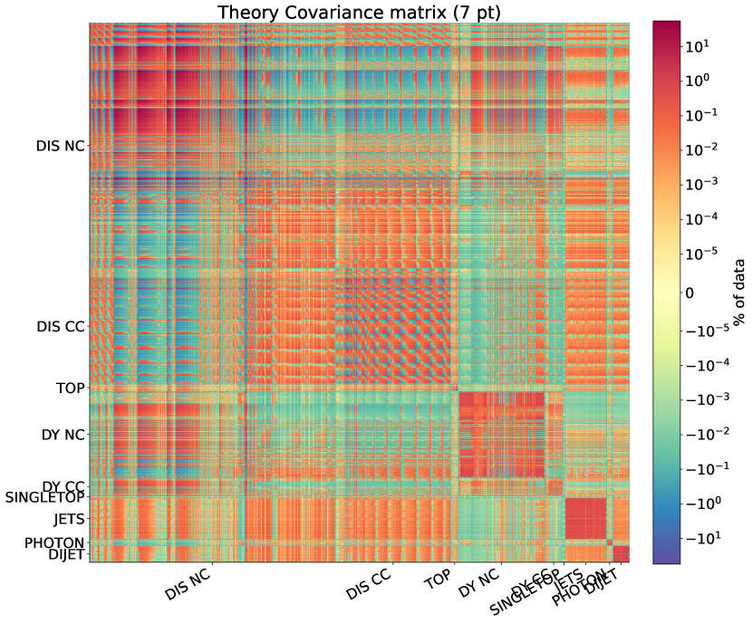
(a) NLO

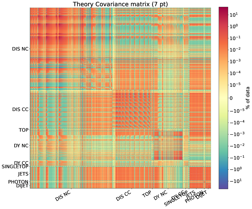
(b) NNLO

Figure 3.1: The MHOU covariance matrix Eq. (2.20) computed with the 7-point prescription at NLO (left) and NNLO (right).

The relative uncertainties on individual points (i.e. the square-root of the diagonal covariance matrix elements) before and after the inclusion of the MHOU and the MHOU itself are compared in Fig. 3.2 at NLO and NNLO. It is clear that at the level of uncertainties at NLO the MHOU uncertainty is comparable to the other components of the uncertainty, whereas at NNLO it is clearly subdominant. Consequently we might expect the effect of MHOUs at NNLO to be mostly through correlations, and thus to mostly impact PDF central values, and less so PDF uncertainties.

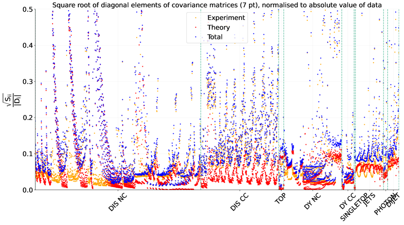
(a) NLO

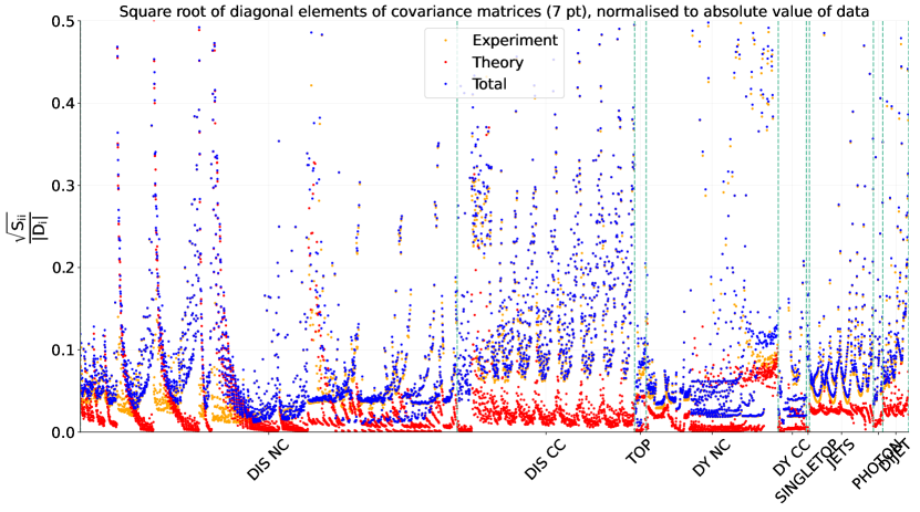
(b) NNLO

Figure 3.2: Comparison of the experimental and MHO contributions to the relative uncertainty, defined as the square root of the diagonal element of the covariance matrix normalized to the value of the theory prediction, at NLO (top) and NNLO (bottom), for all datapoints. The experimental, MHO, and total uncertainties are shown in yellow, red and blue respectively.

3.2 Validation

The MHOU covariance matrix at NLO can be validated by comparing it to the known difference between NLO and NNLO predictions. This comparison can be performed using various estimators, originally proposed in Ref.[11]. We present here results of this validation, both for our default 7-point prescription, as well as for the 9-point prescription discussed in Section 2.3.

We define a normalized shift vector, whose $i$-th component $\delta_{i}$ is the normalized shift of the $i$-th datapoint due to the change in theory prediction from NLO to NNLO for fixed PDF, namely

$$\delta_{i}=\frac{T_{i}^{\text{NNLO}}-T_{i}^{\text{NLO}}}{T_{i}^{\text{NLO}}},$$ (3.1)

where the index $i$ runs over all the datapoints, and $T_{i}^{\text{NNLO}}$ and $T_{i}^{\text{NLO}}$ are respectively the NNLO and NLO theory predictions both computed using the NLO PDF set.

The simplest validation consists of comparing the shift $\delta_{i}$ to the uncertainty on individual points (also normalized), i.e. to the square root of the diagonal entries of the normalized NLO MHOU covariance matrix

$$\hat{S}_{ij}^{\text{NLO}}=\frac{S_{ij}^{\text{NLO}}}{T_{i}^{\text{NLO}}T_{j}^{\text{NLO}}}\,.$$ (3.2)

Results are shown, for both the 7-point and the 9-point prescriptions, in Fig. 3.3, where we compare $\delta_{i}$ to $\pm\sqrt{\hat{S}_{ii}}$. It is clear that for DIS both 7-point and 9-point scale variations at NLO provide a very conservative uncertainty estimate that significantly overestimates the NLO-NNLO shift. On the other hand for hadronic processes the shift and scale variation estimate are generally comparable in size. Only for DY scale variations perform less well, with instances of underestimation of the shift.

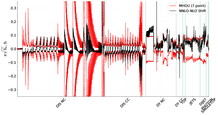
(a) 7 point

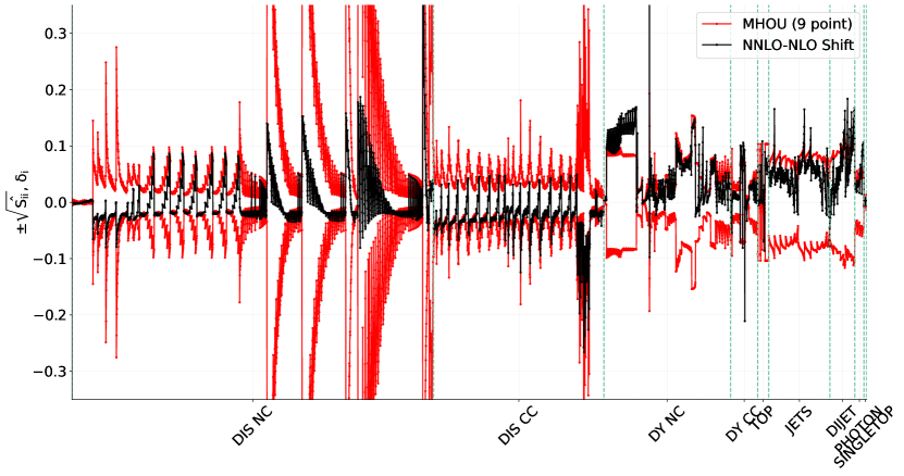
(b) 9 point

Figure 3.3: Comparison of the symmetrized NLO MHOU $\pm{\sqrt{\hat{S}_{ii}}}$ (red, same as in Fig. 3.2, but normalized to the NLO theory prediction) to the normalized NNLO-NLO shift $\delta_{i}$ Eq. (3.1) (black) for all datapoints. Results obtained with the 7-point (top) and 9-point (bottom) prescription are shown.

This validation is however very crude, in that it does not test correlations at all. These can be checked by comparing the eigenvalues of the covariance matrix to the projection of the shift along its eigenvectors. It is important to realize that the shift $\delta_{i}$ is a vector in the $N_{\rm dat}$-dimensional space of data, of which the independent eigenvectors of the covariance matrix span a small subspace $S$ with dimension $N_{\rm sub}\ll N_{\rm dat}$. In our case, $N_{\rm dat}=4616$ while $N_{\rm sub}=22$ for 7-point scale variation, and $N_{\rm sub}=48$ for 9-point (see formulae in Appendix A of Ref. [11] with $p=9$ process classes). Therefore, a further nontrivial requirement is that the shift vector be mostly contained within the subspace $S$.

We can perform both tests quantitatively as follows [11]. First, we determine the eigenvectors $e_{i}^{\alpha}$ and the eigenvalues $\lambda^{\alpha}=(s^{\alpha})^{2}$ of the MHOU covariance matrix, with $s^{\alpha}>0$. Then, we determine the $N_{\rm sub}$ projections $\delta^{\alpha}$ of the shift vector $\delta_{i}$ on the eigenvectors $e_{i}^{\alpha}$, i.e.

$$\delta^{\alpha}=\sum_{i=1}^{N_{\text{dat}}}\delta_{i}e_{i}^{\alpha},\quad\alpha=1,\dots,N_{\rm sub}.$$ (3.3)

Finally, we determine the component of the shift vector in the $N_{\rm sub}$ dimensional subspace $S$:

$$\delta^{S}_{i}=\sum_{\alpha=1}^{N_{\rm sub}}\delta^{\alpha}e_{i}^{\alpha},$$ (3.4)

and the orthogonal component

$$\delta^{\rm miss}_{i}=\delta_{i}-\delta^{S}_{i},$$ (3.5)

which is the part of the shift vector that is missed by the MHOU covariance matrix.

We can now test whether correlated uncertainties are correctly accounted for by checking whether $s^{\alpha}$ are of comparable size of $\delta^{\alpha}$ — in principle, assuming MHO terms to be Gaussianly distributed, 68% of $\delta^{\alpha}$ should be smaller than or equal to $s^{\alpha}$. We can further test how much of the shift vectors lies in the subspace $S$ by determining the length $|\delta^{\rm miss}|$ of the missed vector, and the angle between the full shift vector and its component contained in the $S$ subspace

$$\theta=\arccos{\left(\frac{|\delta^{S}|}{|\delta|}\right)}.$$ (3.6)

Clearly, if the shift was entirely explained by the MHOU covariance matrix, then $|\delta^{\rm miss}|=0$, $|\delta^{S}|=|\delta|$, and $\theta=0$.

The shift projections $|\delta^{\alpha}|$ and covariance matrix eigenvalues $|s^{\alpha}|$ are compared both for the 7-point and the 9-point prescriptions in Fig. 3.4, where we also show the length of the missed component $|\delta^{\rm miss}|$. There is good agreement between shift projections and predicted MHOUs for the largest eigenvalues using both prescriptions. For smaller eigenvectors there is also generally good agreement, but the 9-point prescription somewhat underestimates the size of individual components of the shift.

		DIS NC	DIS CC	TOP	DY NC	DY CC	SINGLETOP	JETS	PHOTON	DIJET	TOTAL
Prescription	$N_{\rm sub}$	$\theta$ [$\degree$]
7-point	22	39	18	24	23	38	14	15	12	12	32
9-point	48	37	15	20	23	34	12	13	7	12	28

Table 3.1: The angle $\theta$, Eq. (3.6), for the 7-point and the 9-point prescriptions for individual process categories and for the total dataset. The dimension $N_{\rm sub}$ of the $S$ subspace is also shown.

The size of the missed component of shift vector can be seen in Fig. 3.4 to be similar to its largest eigenvector component for both prescriptions, i.e. relatively small in comparison to the full shift, given that the first ten components or so are of comparable size. Indeed, this can be seen from the angle Eq. (3.6) between the shift vector and its projection in the subspace $S$, which is tabulated in Tab. 3.1 both for individual datasets and the full dataset. The two prescriptions perform both surprisingly well, given the very small size of the $S$ subspace, with a very small difference between the two prescriptions despite the difference by more than a factor 2 in the size of the $S$ subspace. For almost all datasets the direction of the shift and its projection in the $S$ subspace are quite close and in some cases very close, the only exception being NC DIS and to a lesser extent DY, especially CC.

In summary, we conclude that the NLO MHOU covariance matrix accounts quite well for the uncertainty due to the missing NNLO corrections, with only the uncertainty on the DY prediction somewhat underestimated by scale variation, and the performance of the 7-point and 9-point prescription fairly close. Specifically, the 9-point prescription performs slightly better in terms of capturing the subspace in which the shift lies, while the 7-point performs somewhat better in terms of correctly describing the size of the uncertainty in the subspace. In the sequel we will adopt the 7-point prescription as a default.

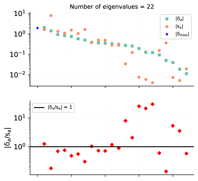
(a) 7-point

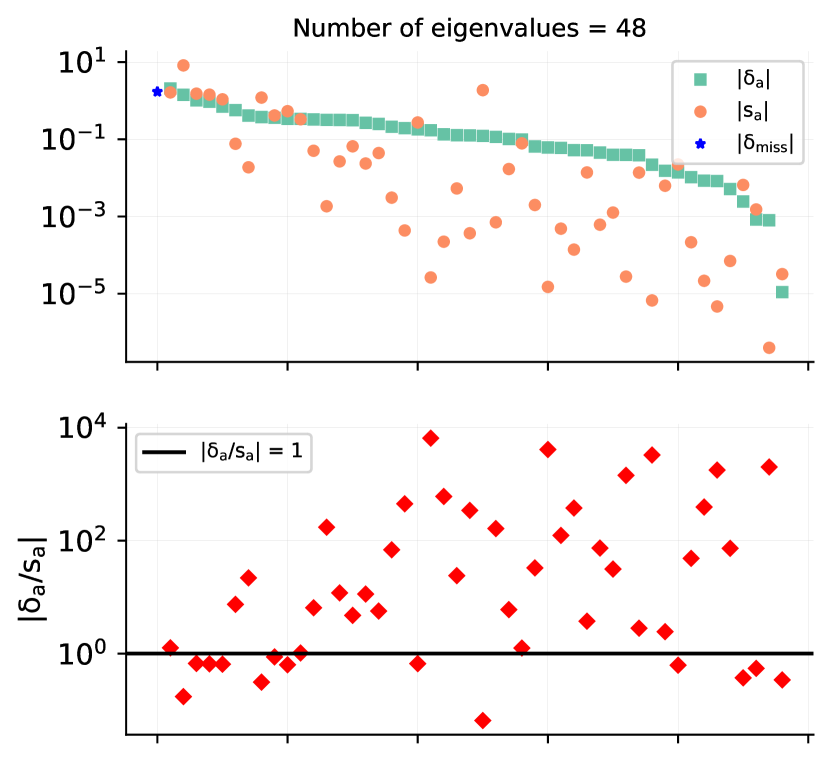
(b) 9-point

Figure 3.4: The projection $|\delta^{\alpha}|$ Eq. 3.3 of the shift vector along each eigenvector of the MHOU covariance matrix compared to the square root $|s^{\alpha}|$ of the corresponding eigenvalue, for both the 7- and the 9-point prescription. The plots are ordered by decreasing size of the projections and the results are shown both as absolute and as a ratio. In the absolute panel, the length $|\delta^{\text{miss}}|$ Eq. (3.5) of the missed component Eq. (3.5) is also shown.

4 The NNPDF4.0MHOU determination

We now turn to the main deliverables of this paper, namely the NNPDF4.0 NLO and NNLO PDF sets with MHOUs, which are obtained by repeating the corresponding NNPDF4.0 PDF determinations, but now also including a MHOU covariance matrix determined with a 7-point prescription, as discussed in Section 2. The underlying dataset is identical to that used for the determination of the NNPDF4.0 NNLO PDFs [1]. As already mentioned in Section 3.1, here we adopt exactly the same dataset at NLO and NNLO, while in Ref. [1] a somewhat different dataset was used at NLO. Hence, we compare here four PDF sets: NLO and NNLO, with and without MHOUs, all determined based on the same underlying data.

Note that the NLO PDFs without MHOUs shown here are unsuitable for phenomenology, because they include data for which NNLO corrections are very large, and were thus excluded from the NNPDF4.0NLO dataset of Ref. [1]. However in this study we prefer to compare PDFs produced using exactly the same code and the same dataset, and that only differ in perturbative order and in the presence of MHOUs, so that the effect of the latter can be assessed without any confounding effect, however small.

Note also that the NNPDF4.0 NNLO without MHOUs shown here are equivalent but not identical to the published NNPDF4.0 PDFs [1]: they differ from them because of the correction of a few minor bugs in the data implementation, and because of the use of a new theory pipeline [15] for the computation of predictions, which in particular includes a new implementation of the treatment of heavy quark mass effects that differs from the previous one by subleading terms. The impact of these changes was assessed in Appendix A of Ref. [16], and was found to be very limited, so that for any application the NNPDF4.0 NNLO MHOU PDFs presented here can be considered to be the counterpart of the published NNPDF4.0 NNLO PDFs (without MHOU) [1].

4.1 Fit quality

In Tabs. 4.1-4.4 we report the number of data points and the $\chi^{2}$ per data point in the NLO and NNLO NNPDF4.0 PDF determinations before and after inclusion of MHOUs. When MHOUs are not included, the covariance matrix is defined as in Ref. [1], namely, it is the sum of the experimental covariance matrix $C$ and of a theory covariance matrix accounting for missing nuclear corrections $S^{\rm(nucl)}$, as determined in Refs. [8, 9], and whose impact is discussed in Section 8.6 of Ref. [1]. When MHOUs are included, the covariance matrix also contains the contribution Eq. (2.20) discussed in Sections 2.3-3.1, that we call $S^{\rm(7pt)}$.

Note that the MHOU contribution is respectively excluded or included both in the definition of the $\chi^{2}$ used by the NNPDF algorithm (i.e. for pseudodata generation and in training and validation loss functions), and in the covariance matrix used in order to compute the values given in Tabs. 4.1-4.4. Note also that the experimental covariance matrix used in order to compute the values given in Tabs. 4.1-4.4 differs from that used in the NNPDF algorithm, because the latter treats multiplicative uncertainties according to the $t_{0}$ method [40] in order to avoid the d’Agostini bias, while the former is just the published experimental covariance matrix. In Tab. 4.1 datasets are aggregated according to the process categorization of Section 3.1. Individual data sets are displayed in Tab. 4.2 (NC and CC DIS), in Tab. 4.3 (NC and CC DY), and in Tab. 4.4 (top pairs, single-inclusive jets, dijets, isolated photons, and single top). The naming of the datasets follows Ref. [1].

Dataset	$N_{\rm dat}$	NLO		NNLO
		$C+S^{\rm(nucl)}$	$C+S^{\rm(nucl)}+S^{\rm(7pt)}$	$C+S^{\rm(nucl)}$	$C+S^{\rm(nucl)}+S^{\rm(7pt)}$
DIS NC	2100	1.30	1.22	1.23	1.20
DIS CC	989	0.92	0.87	0.90	0.90
DY NC	736	2.01	1.71	1.20	1.15
DY CC	157	1.48	1.42	1.48	1.37
Top pairs	64	2.08	1.24	1.21	1.43
Single-inclusive jets	356	0.84	0.82	0.96	0.81
Dijets	144	1.52	1.84	2.04	1.71
Prompt photons	53	0.59	0.49	0.75	0.67
Single top	17	0.36	0.35	0.36	0.38
Total	4616	1.34	1.23	1.17	1.13

Table 4.1: The number of data points and the $\chi^{2}$ per data point for the NLO and NNLO NNPDF4.0 PDF sets without and with MHOUs. Datasets are grouped according to the process categorization of Section 3.1.

Dataset	$N_{\rm dat}$	NLO		NNLO
		$C+S^{\rm(nucl)}$	$C+S^{\rm(nucl)}+S^{\rm(7pt)}$	$C+S^{\rm(nucl)}$	$C+S^{\rm(nucl)}+S^{\rm(7pt)}$
NMC $F_{2}^{d}/F_{2}^{p}$	121	0.87	0.87	0.87	0.88
NMC $\sigma^{{\rm NC},p}$	204	1.96	1.29	1.62	1.33
SLAC $F_{2}^{p}$	33	1.72	0.84	0.97	0.68
SLAC $F_{2}^{d}$	34	1.08	0.75	0.63	0.54
BCDMS $F_{2}^{p}$	333	1.60	1.26	1.41	1.29
BCDMS $F_{2}^{d}$	248	1.06	1.01	1.01	0.99
HERA I+II $\sigma_{\rm NC}\ e^{-}p$	159	1.39	1.39	1.39	1.39
HERA I+II $\sigma_{\rm NC}\ e^{+}p$ ($E_{p}=460$ GeV)	204	1.11	1.04	1.08	1.04
HERA I+II $\sigma_{\rm NC}\ e^{+}p$ ($E_{p}=575$ GeV)	254	0.89	0.87	0.92	0.88
HERA I+II $\sigma_{\rm NC}\ e^{+}p$ ($E_{p}=820$ GeV)	70	1.08	0.96	1.12	0.95
HERA I+II $\sigma_{\rm NC}\ e^{+}p$ ($E_{p}=920$ GeV)	377	1.19	1.17	1.30	1.25
HERA I+II $\sigma_{\rm NC}^{c}$	37	1.83	1.66	2.03	1.75
HERA I+II $\sigma_{\rm NC}^{b}$	26	1.46	1.03	1.45	1.11
CHORUS $\sigma_{CC}^{\nu}$	416	0.96	0.95	0.97	0.97
CHORUS $\sigma_{CC}^{\bar{\nu}}$	416	0.90	0.87	0.88	0.87
NuTeV $\sigma_{CC}^{\nu}$ (dimuon)	39	0.22	0.22	0.31	0.33
NuTeV $\sigma_{CC}^{\bar{\nu}}$ (dimuon)	37	0.58	0.39	0.56	0.64
HERA I+II $\sigma_{\rm CC}\ e^{-}p$	42	1.39	1.18	1.25	1.29
HERA I+II $\sigma_{\rm CC}\ e^{+}p$	39	1.33	1.25	1.22	1.25

Table 4.2: Same as Tab. 4.1, for the DIS NC (top) and DIS CC (bottom) datasets.

Dataset	$N_{\rm dat}$	NLO		NNLO
		$C+S^{\rm(nucl)}$	$C+S^{\rm(nucl)}+S^{\rm(7pt)}$	$C+S^{\rm(nucl)}$	$C+S^{\rm(nucl)}+S^{\rm(7pt)}$
E866 $\sigma^{d}/2\sigma^{p}$ (NuSea)	15	0.66	0.52	0.53	0.51
E866 $\sigma^{p}$ (NuSea)	29	1.35	0.85	1.63	1.00
E605 $\sigma^{d}/2\sigma^{p}$ (NuSea)	85	0.44	0.42	0.46	0.45
E906 $\sigma^{d}/2\sigma^{p}$ (SeaQuest)	6	1.23	3.20	0.90	0.90
CDF $Z$ differential	28	1.36	1.26	1.23	1.18
D0 $Z$ differential	28	0.75	0.73	0.64	0.64
ATLAS low-mass DY 7 TeV	6	13.3	8.97	0.87	0.78
ATLAS high-mass DY 7 TeV	5	1.60	1.64	1.60	1.67
ATLAS $Z$ 7 TeV ($\mathcal{L}=35$ pb-1)	8	0.77	0.49	0.60	0.57
ATLAS $Z$ 7 TeV ($\mathcal{L}=4.6$ fb-1) CC	24	5.00	3.29	1.73	1.68
ATLAS $W,Z$ 7 TeV ($\mathcal{L}=4.6$ fb-1) CF	15	1.82	1.21	1.07	1.02
ATLAS low-mass DY 2D 8 TeV	60	1.73	1.04	1.21	1.08
ATLAS high-mass DY 2D 8 TeV	48	1.48	1.34	1.12	1.08
ATLAS $\sigma_{Z}^{\rm tot}$ 13 TeV	1	0.48	0.43	0.30	0.60
ATLAS $Z$ $p_{T}$ 8 TeV ($p_{T},m_{\ell\ell}$)	44	1.05	0.93	0.90	0.91
ATLAS $Z$ $p_{T}$ 8 TeV ($p_{T},y_{Z}$)	48	0.74	0.69	0.88	0.70
CMS DY 2D 7 TeV	110	3.66	1.10	1.35	1.32
CMS $Z$ $p_{T}$ 8 TeV	28	1.66	1.58	1.40	1.41
LHCb $Z\to ee$ 7 TeV	9	1.51	1.36	1.64	1.53
LHCb $Z\to\mu$ 7 TeV	15	1.01	0.85	0.78	0.73
LHCb $Z\to ee$ 8 TeV	17	1.67	1.21	1.25	1.26
LHCb $Z\to\mu$ 8 TeV	16	1.40	1.05	1.46	1.59
LHCb $Z\to ee$ 13 TeV	16	1.34	1.61	0.96	1.80
LHCb $Z\to\mu\mu$ 13 TeV	15	1.88	1.13	1.75	0.99
D0 $W$ muon asymmetry	9	2.48	1.92	1.99	1.95
ATLAS $W$ 7 TeV ($\mathcal{L}=35$ pb-1)	22	1.23	1.15	1.13	1.12
ATLAS $W$ 7 TeV ($\mathcal{L}=4.6$ fb-1)	22	2.74	2.26	2.15	2.16
ATLAS $\sigma_{W}^{\rm tot}$ 13 TeV	2	0.10	0.40	1.21	1.60
ATLAS $W^{+}$+jet 8 TeV	15	1.68	1.15	0.79	0.79
ATLAS $W^{-}$+jet 8 TeV	15	1.82	1.31	1.49	1.45
CMS $W$ electron asymmetry 7 TeV	11	0.85	0.96	0.83	0.85
CMS $W$ muon asymmetry 7 TeV	11	2.05	1.75	1.74	1.73
CMS $W$ rapidity 8 TeV	22	0.92	0.71	1.39	1.03
LHCb $W\to\mu$ 7 TeV	14	1.76	1.44	2.76	1.99
LHCb $W\to\mu$ 8 TeV	14	0.76	0.51	0.96	0.92

Table 4.3: Same as Tab. 4.1, for the DY NC (top) and DY CC (bottom) datasets.

Dataset	$N_{\rm dat}$	NLO		NNLO
		$C+S^{\rm(nucl)}$	$C+S^{\rm(nucl)}+S^{\rm(7pt)}$	$C+S^{\rm(nucl)}$	$C+S^{\rm(nucl)}+S^{\rm(7pt)}$
ATLAS $\sigma_{tt}^{\rm tot}$ 7 TeV	1	11.7	3.66	4.66	2.40
ATLAS $\sigma_{tt}^{\rm tot}$ 8 TeV	1	2.28	0.87	0.03	0.03
ATLAS $\sigma_{tt}^{\rm tot}$ 13 TeV ($\mathcal{L}$=139 fb-1)	1	4.58	1.18	0.56	0.41
ATLAS $t\bar{t}~{}\ell$+jets 8 TeV ($1/\sigma d\sigma/dy_{t}$)	4	3.39	1.89	3.01	3.70
ATLAS $t\bar{t}~{}\ell$+jets 8 TeV ($1/\sigma d\sigma/dy_{t\bar{t}}$)	4	7.19	3.85	3.65	5.80
ATLAS $t\bar{t}~{}2\ell$ 8 TeV ($1/\sigma d\sigma/dy_{t\bar{t}}$)	4	1.80	1.76	1.57	1.86
CMS $\sigma_{tt}^{\rm tot}$ 5 TeV	1	0.72	0.95	0.01	0.01
CMS $\sigma_{tt}^{\rm tot}$ 7 TeV	1	6.37	1.82	1.10	0.50
CMS $\sigma_{tt}^{\rm tot}$ 8 TeV	1	4.39	1.21	0.31	0.17
CMS $\sigma_{tt}^{\rm tot}$ 13 TeV	1	1.06	0.36	0.04	0.01
CMS $t\bar{t}~{}\ell$+jets 8 TeV ($1/\sigma d\sigma/dy_{t\bar{t}}$)	9	1.67	1.61	1.20	1.59
CMS $t\bar{t}$ 2D $2\ell$ 8 TeV ($1/\sigma d\sigma/dy_{t}dm_{t\bar{t}}$)	15	2.03	1.84	1.32	1.25
CMS $t\bar{t}~{}2\ell$ 13 TeV ($d\sigma/dy_{t}$)	10	0.77	0.71	0.51	0.59
CMS $t\bar{t}~{}\ell$+jet 13 TeV ($d\sigma/dy_{t}$)	11	0.54	0.26	0.56	0.66
ATLAS incl. jets 8 TeV, $R=0.6$	171	0.70	0.73	0.71	0.64
CMS incl. jets 8 TeV	185	0.97	0.81	1.19	0.95
ATLAS dijets 7 TeV, $R=0.6$	90	1.48	1.82	2.16	1.69
CMS dijets 7 TeV	54	1.59	2.07	1.84	1.74
ATLAS isolated $\gamma$ prod. 13 TeV	53	0.59	0.50	0.75	0.67
ATLAS single $t$ $R_{t}$ 7 TeV	1	0.38	0.30	0.48	0.57
ATLAS single $t$ $R_{t}$ 13 TeV	1	0.05	0.03	0.06	0.07
ATLAS single $t$ 7 TeV ($1/\sigma d\sigma/dy_{t}$)	3	0.84	0.82	0.97	0.94
ATLAS single $t$ 7 TeV ($1/\sigma d\sigma/dy_{\bar{t}}$)	3	0.06	0.06	0.06	0.06
ATLAS single $t$ 8 TeV ($1/\sigma d\sigma/dy_{t}$)	3	0.35	0.33	0.24	0.26
ATLAS single $t$ 8 TeV ($1/\sigma d\sigma/dy_{\bar{t}}$)	3	0.19	0.21	0.19	0.19
CMS single $t$ $\sigma_{t}+\sigma_{\bar{t}}$ 7 TeV	1	0.91	0.96	0.76	0.84
CMS single $t$ $R_{t}$ 8 TeV	1	0.13	0.09	0.17	0.20
CMS single $t$ $R_{t}$ 13 TeV	1	0.32	0.28	0.35	0.38

Table 4.4: Same as Tab. 4.1, for (from top to bottom) top pair, single-inclusive jet, isolated photon and single top production.

Tables 4.1-4.4 show that upon inclusion of the MHOU covariance matrix the total $\chi^{2}$ decreases for both the NLO and NNLO fits, but the decrease is more substantial at NLO. Even after inclusion of the MHOU, the NLO $\chi^{2}$ remains somewhat higher than the NNLO one. Inspection of Tab. 4.2-4.4 shows that this is in fact due to a small number of datasets (specifically ATLAS low-mass Drell-Yan), and we have further verified that this is in turn due to a small number of very accurately measured data points (excluded by the NLO cuts of Ref. [1]) for which NNLO corrections are very substantially underestimated by scale variation. However, for the majority of datapoints and of process categories, the MHOU covariance matrix correctly accounts for the mismatch between data and theory predictions at NLO due to missing NNLO terms, consistently with the validation of Section 3.2.

4.2 PDFs and PDF uncertainties

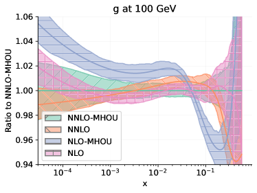
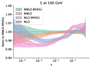
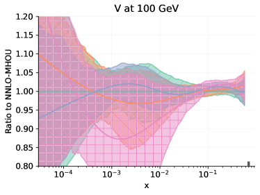
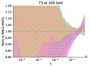
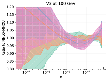
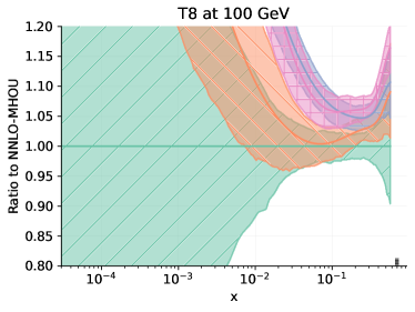
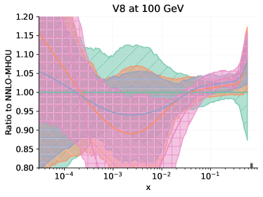
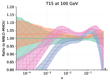
Figure 4.1: The NLO and NNLO PDFs with and without MHOUs at $Q=100$ GeV determined in this work. The gluon, singlet, valence ($V$, $V_{3}$, $V_{8}$), and triplet ($T_{3}$, $T_{8}$, $T_{15}$) PDFs are shown. All curves are normalized to the NNLO with MHOUs. The bands correspond to one sigma uncertainty.

Individual PDFs at NLO and NNLO, with and without MHOUs, are compared in Fig. 4.1 at $Q=100$ GeV. We show the gluon, singlet, valence ($V$, $V_{3}$, $V_{8}$), and triplet ($T_{3}$, $T_{8}$, $T_{15}$) distributions (see Section 3.1.1 of Ref. [1]), all shown as a ratio to the NNLO PDFs with MHOUs. The corresponding one sigma uncertainties are shown in Fig. 4.2. The change in central value due to the inclusion of MHOUs is generally moderate at NNLO; at NLO it is significant for the gluon and singlet, but quite moderate for all other PDF combinations.

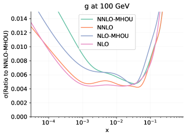
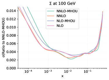
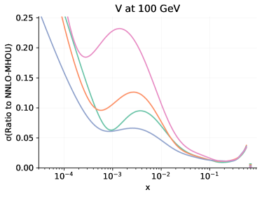
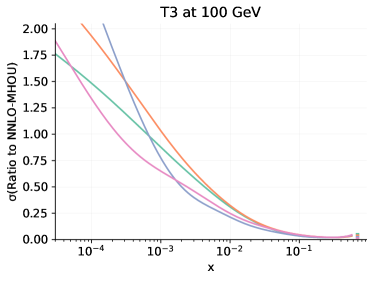
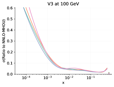
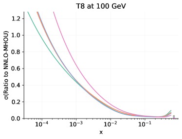
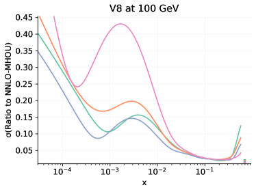
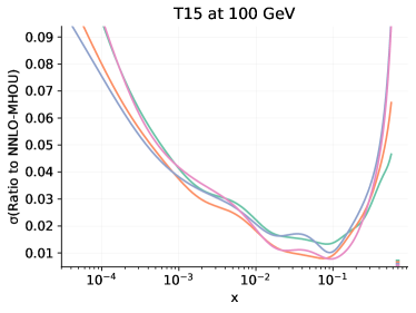
Figure 4.2: Relative one sigma uncertainties for the PDFs shown in Fig. 4.1. All uncertainties are normalized to the corresponding central NNLO PDFs with MHOUs.

The PDF uncertainty at NNLO is generally somewhat reduced or unchanged by the inclusion of MHOUs. The somewhat counter-intuitive fact that the uncertainty on the PDF is reduced upon inclusion of an extra source of uncertainty in the $\chi^{2}$ was already observed in Refs. [8, 9] and demonstrates the increased compatibility of the data due to the MHOU. At NLO a similar effect is observed in the nonsinglet sector, but not in the singlet sector, where the PDF uncertainty increases upon inclusion of the MHOU, consistently with the observation of Sect. 4.1 that at NLO the MHOU from scale variation does not fully account for the large shift from NLO to NNLO for some datasets.

Dataset	NLO		NNLO
	$C+S^{\rm(nucl)}$	$C+S^{\rm(nucl)}+S^{\rm(7pt)}$	$C+S^{\rm(nucl)}$	$C+S^{\rm(nucl)}+S^{\rm(7pt)}$
DIS NC	0.14	0.13	0.15	0.13
DIS CC	0.12	0.12	0.12	0.12
DY NC	0.19	0.17	0.18	0.17
DY CC	0.37	0.30	0.35	0.32
Top pairs	0.19	0.16	0.17	0.17
Single-inclusive jets	0.13	0.12	0.13	0.13
Dijets	0.10	0.09	0.11	0.10
Prompt photon	0.06	0.06	0.06	0.06
Single top	0.04	0.04	0.04	0.04
Total	0.16	0.15	0.17	0.15

Table 4.5: The $\phi$ uncertainty estimator for PDFs at NLO and NNLO with and without MHOUs for the process categories of Section 3.1.

A quantitative assessment of PDF uncertainties on physics predictions can be obtained through the $\phi$ estimator, which was introduced in Ref. [41] (see Eq. (4.6) there), and gives the ratio of the average correlated PDF uncertainty over the data uncertainty. As such, it provides an estimate of the consistency of the data: consistent data are combined by the underlying theory and lead to an uncertainty in the prediction which is smaller than that of the original data (see also the discussion in Section 6 of Ref. [12]). The value of $\phi$ before and after inclusion of the MHOUs is shown at NLO and NNLO in Tab. 4.5. It is clear that $\phi$ decreases upon inclusion of MHOUs for most data categories, more substantially at NNLO, and by a smaller amount at NLO. This further confirms that at NNLO data compatibility is increased by the inclusion of PDF uncertainties, but this is not always the case at NLO.

A priori, PDF sets with and without MHOUs should not necessarily be compatible within uncertainties, given that the latter do not include an existing source of uncertainty. As a matter of fact, they do agree in the nonsinglet sector, where MHOU are at most of about the same size as the PDF uncertainty before inclusion of MHOUs, but they generally do not in the singlet sector, where NNLO corrections can be very large.

Inclusion of MHOUs generally moves the NLO PDFs towards the NNLO, thereby improving perturbative convergence, except for the gluon. In fact, even for the singlet, while the NLO moves towards the NNLO upon inclusion of MHOUs, the NNLO result remains well outside the NLO uncertainty band, especially at small $x$. Again, this shows that in the singlet sector there are large NNLO corrections to the NLO result that are underestimated by MHOUs determined through scale variation. At small $x$ this can be understood as the consequence of unresummed small-$x$ logarithms [42] whose increase with perturbative order is not accounted for by scale variation.

The general conclusion is thus that the inclusion of MHOUs estimated through scale variation at NNLO improves data compatibility resulting in some reduction of uncertainties and a moderate shift of central values. At NLO it manages to account for the effect of MHOUs in fit quality while having a moderate impact on either PDF uncertainties and central values in the nonsinglet sector, and a more significant impact on central values with an increase in uncertainties in the singlet sector, while not fully accounting for the largest missing NNLO corrections.

5 Delivery and outlook

We have presented NLO and NNLO sets of parton distributions for which the PDF uncertainty includes not only the uncertainty coming from the data and that from the analysis methodology used to go from the data to the PDFs, but also the uncertainty coming from the perturbative truncation of the computations used in order to get the theory predictions that are compared to data (MHOUs). We followed the methodology that was developed in Refs. [11, 12] and used there to construct the first NLO PDF sets including MHOUs. This methodology can now be used to determine MHOUs up to N³LO, thanks to the availability of the EKO evolution code [14], and the interfacing of the NNPDF code [43] both to it and to flexible tools for the computation of physical processes (such as the YADISM module [44] for DIS) through a new and streamlined theory pipeline [15].

The MHOUs on PDFs discussed in this paper should be treated as an extra contribution to the PDF uncertainty: they reflect the uncertainty in the theory predictions used in PDF determination and are thus on a par with the experimental uncertainty on the data themselves. They are consequently independent of the further MHOU on the hard cross-section of the processes which are being predicted. The total uncertainty on predictions must therefore be obtained by combining the PDF uncertainty, now also including a MHOU component, with the MHOU uncertainty on the hard cross section computation. The latter is typically determined as the envelope of a 7-point scale variation (see e.g. Ref. [45]). However, it is also possible to include MHOUs on the hard cross section by constructing a theory covariance matrix for the hard corss section itself. An advantage of doing so is that it is then also possible to keep into account the correlation between the theory uncertainty in the process used for PDF determination, and that on the hard cross-section, which might become relevant if the experimental uncertainties are small and the predicted process was also used for PDF determination [46, 22]. This can be done by determining the cross-correlation of MHO and PDF uncertainties between the predicted process and those used for PDF determination [47].

In this respect, it is interesting to observe that an altogether different option for the inclusion of MHOUs on predictions that accounts for MHOUs on PDFs, and their full correlation to MHOUs on the hard cross-sections, is to include the scale variation in the Monte Carlo sampling [22]. A comparative study of this methodology to that adopted in the present paper, as well of different prescriptions for scale variation (such as, for instance different prescrriptions for the connstruction of the theory covariance matrix of Sect. 2.3) will be left for future studies.

The NNPDF4.0MHOU NNLO PDF set is made publicly available via the LHAPDF6 interface,

http://lhapdf.hepforge.org/  .

It is delivered as a set of $N_{\rm rep}=100$ Monte Carlo replicas, and it is denoted as

NNPDF40_nnlo_as_01180_mhou

It should be considered a more accurate version of the published NNPDF4.0 NNLO PDF set [1].

This PDF set is also made available via the NNPDF collaboration website

https://nnpdf.mi.infn.it/nnpdf4-0-mhou/  ,

where we also make available the other PDF sets presented in Section 4. These include the NLO PDFs with MHOUs based on the same dataset used at NNLO

NNPDF40_nlo_as_01180_mhou_nocuts

and the corresponding baseline NLO and NNLO sets without MHOUs

NNPDF40_nlo_as_01180_qcd_nocuts
NNPDF40_nnlo_as_01180_qcd .

The latter NNLO set is equivalent to but differs from the published NNPDF4.0 NNLO because of the adoption of a new theory pipeline, and was already presented in Ref. [16] (see in particular Appendix A of that reference).

The availability of PDFs that include MHOUs in their uncertainty is a step forward in achieving high-accuracy PDFs that can be used for precision phenomenology at the percent level. We will soon extend the results presented here to approximate N³LO [48] (for which approximate results are already available [23]). This will allow us to discuss the convergence of the perturbative expansion both of PDFs and perturbative observables, and the effect of the inclusion of MHOUs upon it. Further detailed studies of the phenomenological implications of the NNPDF4.0 PDFs, including MHOUs and the approximate N³LO PDFs, are left for future studies [49].

Acknowledgments

R. D. B, L. D. D., and R. S. are supported by the U.K. Science and Technology Facility Council (STFC) grant ST/T000600/1. F. H. is supported by the Academy of Finland project 358090 and is funded as a part of the Center of Excellence in Quark Matter of the Academy of Finland, project 346326. E. R. N. is supported by the Italian Ministry of University and Research (MUR) through the “Rita Levi-Montalcini” Program. M. U. and Z. K. are supported by the European Research Council under the European Union’s Horizon 2020 research and innovation Programme (grant agreement n.950246), and partially by the STFC consolidated grant ST/T000694/1 and ST/X000664/1. J. R. is partially supported by NWO, the Dutch Research Council. C. S. is supported by the German Research Foundation (DFG) under reference number DE 623/6-2.

Appendix A Expansion coefficients

We give here explicit expressions for the perturbative expansion coefficients that are needed in order to perform scale variation according to the prescriptions discussed in Section 2. Even though in this paper we only present results up to NNLO, expressions up to N³LO are given for future reference.

Running of $a_{s}$.

The perturbative solution of Eq. 2.4 is

$$a_{s}(\lambda\mu^{2}) =a_{s}(\mu^{2})-\left(a_{s}(\mu^{2})\right)^{2}\beta_{0}\ln\lambda+\left(a_{s}(\mu^{2})\right)^{3}\left(\left(\beta_{0}\right)^{2}\ln^{2}\lambda-\beta_{1}\ln\lambda\right)$$

$$\hskip 20.0pt-\left(a_{s}(\mu^{2})\right)^{4}\left(\left(\beta_{0}\right)^{3}\ln^{3}\lambda-\frac{5}{2}\beta_{0}\beta_{1}\ln^{2}\lambda+\beta_{2}\ln\lambda\right)$$

$$\hskip 20.0pt+O\left(\left(a_{s}(\mu^{2})\right)^{5}\right).$$ (A.1)

PDF evolution.

The perturbative solution of Eq. 2.5 is

$$E(\lambda\mu^{2}\leftarrow\mu^{2}) =\mathbbm{1}-a_{s}(\mu^{2})\gamma_{0}\ln\lambda+\left(a_{s}(\mu^{2})\right)^{2}\left[\frac{1}{2}\gamma_{0}\left(\beta_{0}+\gamma_{0}\right)\ln^{2}\lambda-\gamma_{1}\ln\lambda\right]$$

$$\hskip 20.0pt-\left(a_{s}(\mu^{2})\right)^{3}\left[\frac{1}{6}\gamma_{0}\left(2\left(\beta_{0}\right)^{2}+3\beta_{0}\gamma_{0}+\left(\gamma_{0}\right)^{2}\right)\ln^{3}\lambda\right.$$

$$\hskip 90.0pt-\left.\frac{1}{6}\left(\beta_{1}\gamma_{0}+2\beta_{0}\gamma_{1}+\gamma_{0}\gamma_{1}+\gamma_{1}\gamma_{0}\right)\ln^{2}\lambda+\gamma_{2}\ln\lambda\right]$$

$$\hskip 20.0pt+{\cal O}\left(\left(a_{s}(\mu^{2})\right)^{4}\right)\,.$$ (A.2)

Scale variation of cross-sections and anomalous dimensions.

The expression of the scale-varied coefficients $\bar{C}_{j}(\rho)$ Eq. (2.10) in terms of the expansion coefficients $C_{j}$ Eq. (2.3) is

$$\bar{C}_{0}(\rho) =C_{0}\,,$$ (A.3)

$$\bar{C}_{1}(\rho) =C_{1}+mC_{0}\beta_{0}\ln\rho\,,$$ (A.4)

$$\bar{C}_{2}(\rho) =C_{2}+\frac{m(m+1)}{2}C_{0}\left(\beta_{0}\right)^{2}\ln^{2}\rho+\left((m+1)C_{1}\beta_{0}+mC_{0}\beta_{1}\right)\ln\rho\,,$$ (A.5)

$$\bar{C}_{3}(\rho) =C_{3}+\frac{m(m+1)(m+2)}{6}C_{0}\left(\beta_{0}\right)^{3}\ln^{3}\rho$$

$$\hskip 20.0pt+\left(\frac{(m+1)(m+2)}{2}C_{1}\left(\beta_{0}\right)^{2}+\frac{m(2m+3)}{2}C_{0}\beta_{0}\beta_{1}\right)\ln^{2}\rho$$

$$\hskip 20.0pt+\left((m+2)C_{2}\beta_{0}+(m+1)C_{1}\beta_{1}+mC_{0}\beta_{2}\right)\ln\rho\,.$$ (A.6)

The expression for of the scale-varied coefficients $\bar{\gamma}_{j}(\rho)$ Eq. (2.12) in terms of the expansion coefficients $\gamma_{j}$ Eq. (2.7) of course is the same, with $m=1$ and $C\rightarrow\gamma$.

Scale variation of PDFs.

The expression of the coefficients $K_{j}(\rho)$ Eq. 2.16 in terms of the expansion coefficients $\gamma_{j}$ Eq. (2.7) can be obtained by setting $\lambda=1/\rho$ in Eq. (A.2). They are given by

$$K_{0}(\rho) =\mathbbm{1}\,,$$ (A.7)

$$K_{1}(\rho) =\gamma_{0}\ln\rho\,,$$ (A.8)

$$K_{2}(\rho) =\frac{1}{2}\gamma_{0}\left(\beta_{0}+\gamma_{0}\right)\ln^{2}\rho+\gamma_{1}\ln\rho\,,$$ (A.9)

$$K_{3}(\rho) =\frac{1}{6}\gamma_{0}\left(2\left(\beta_{0}\right)^{2}+3\beta_{0}\gamma_{0}+\left(\gamma_{0}\right)^{2}\right)\ln^{3}\rho$$

$$\hskip 20.0pt+\frac{1}{2}\left(\beta_{1}\gamma_{0}+2\beta_{0}\gamma_{1}+\gamma_{0}\gamma_{1}+\gamma_{1}\gamma_{0}\right)\ln^{2}\rho+\gamma_{2}\ln\rho\,.$$ (A.10)

Factorization scale variation in coefficient functions.

Substituting Eq. (2.18) in Eq. (2.2) the factorized expression for the physical observable after factorization scale variation is

$$F(Q^{2}) =C(Q^{2})\bar{f}(Q^{2},\rho_{f})$$

$$=C(Q^{2})K(a_{s}(\rho_{f}Q^{2}),\rho_{f})E(\rho_{f}Q^{2}\leftarrow\mu^{2}_{0})f(\mu_{0}^{2})$$ (A.11)

$$=\bar{\bar{C}}(Q^{2},\rho_{f})f(\rho_{f}Q^{2})\left[1+O(a_{s})\right],$$ (A.12)

where we defined

$$\bar{\bar{C}}(Q^{2},\rho_{f})=C(Q^{2})K^{\prime}(a_{s}(Q^{2}),\rho_{f})=\alpha_{s}^{m}(Q^{2})\sum_{j=0}^{k}\left(a_{s}(Q^{2})\right)^{j}\bar{\bar{C}}_{j}(\rho_{f}),$$ (A.13)

and $K^{\prime}$ is in turn found by re-expressing $K(\rho_{f}Q^{2},\rho_{f})$ as a series in $a_{s}(Q^{2})$, namely letting

$$K^{\prime}(a_{s}(Q^{2}),\rho_{f})=\sum_{j=0}^{k}\left(a_{s}(Q^{2})\right)^{j}K^{\prime}_{j}(\rho_{f})$$ (A.14)

with the requirement

$$K(a_{s}(\rho_{f}Q^{2}),\rho_{f})=K^{\prime}(a_{s}(Q^{2}),\rho_{f})\left[1+O(a_{s})\right].$$ (A.15)

We get

$$K^{\prime}_{0}(\rho) =\mathbbm{1}\,,$$ (A.16)

$$K^{\prime}_{1}(\rho) =\gamma_{0}\ln\rho,$$ (A.17)

$$K^{\prime}_{2}(\rho) =\frac{1}{2}\gamma_{0}\left(-\beta_{0}+\gamma_{0}\right)\ln^{2}\rho+\gamma_{1}\ln\rho\,,$$ (A.18)

$$K^{\prime}_{3}(\rho) =\frac{1}{6}\gamma_{0}\left(2\left(\beta_{0}\right)^{2}-3\beta_{0}\gamma_{0}+\left(\gamma_{0}\right)^{2}\right)\ln^{3}\rho$$

$$\hskip 20.0pt+\frac{1}{2}\left(-\beta_{1}\gamma_{0}-2\beta_{0}\gamma_{1}+\gamma_{0}\gamma_{1}+\gamma_{1}\gamma_{0}\right)\ln^{2}\rho+\gamma_{2}\ln\rho\,,$$ (A.19)

which, substituted in Eq. (A.13) leads to

$$\bar{\bar{C}}_{0}(\rho) =C_{0}\,,$$ (A.20)

$$\bar{\bar{C}}_{1}(\rho) =C_{1}+\gamma_{0}C_{0}\ln\rho\,,$$ (A.21)

$$\bar{\bar{C}}_{2}(\rho) =C_{2}+\frac{1}{2}\gamma_{0}(-\beta_{0}+\gamma_{0})C_{0}\ln^{2}\rho+\left(\gamma_{0}C_{1}+\gamma_{1}C_{0}\right)\ln\rho\,,$$ (A.22)

$$\bar{\bar{C}}_{3}(\rho) =C_{3}+\frac{1}{6}\gamma_{0}\left(2\left(\beta_{0}\right)^{2}-3\beta_{0}\gamma_{0}+\left(\gamma_{0}\right)^{2}\right)C_{0}\ln^{3}\rho$$

$$\hskip 20.0pt+\frac{1}{2}\left(-\beta_{1}\gamma_{0}-2\beta_{0}\gamma_{1}+\gamma_{0}\gamma_{1}+\gamma_{1}\gamma_{0}\right)C_{0}\ln^{2}\rho$$

$$\hskip 20.0pt+\frac{1}{2}\gamma_{0}\left(-\beta_{0}+\gamma_{0}\right)C_{1}\ln^{2}\rho$$

$$\hskip 20.0pt+\left(\gamma_{0}C_{2}+\gamma_{1}C_{1}+\gamma_{2}C_{0}\right)\ln\rho\,.$$ (A.23)

References

- [1] NNPDF Collaboration, R. D. Ball et al., The path to proton structure at 1% accuracy, Eur. Phys. J. C 82 (2022), no. 5 428, [arXiv:2109.02653].
- [2] L. Del Debbio, T. Giani, and M. Wilson, Bayesian approach to inverse problems: an application to NNPDF closure testing, Eur. Phys. J. C 82 (2022), no. 4 330, [arXiv:2111.05787].
- [3] NNPDF Collaboration, R. D. Ball, J. Cruz-Martinez, L. Del Debbio, S. Forte, Z. Kassabov, E. R. Nocera, J. Rojo, R. Stegeman, and M. Ubiali, Response to ”Parton distributions need representative sampling”, arXiv:2211.12961.
- [4] T.-J. Hou et al., New CTEQ global analysis of quantum chromodynamics with high-precision data from the LHC, Phys. Rev. D 103 (2021), no. 1 014013, [arXiv:1912.10053].
- [5] S. Bailey, T. Cridge, L. A. Harland-Lang, A. D. Martin, and R. S. Thorne, Parton distributions from LHC, HERA, Tevatron and fixed target data: MSHT20 PDFs, Eur. Phys. J. C 81 (2021), no. 4 341, [arXiv:2012.04684].
- [6] S. Alekhin, J. Blümlein, S. Moch, and R. Placakyte, Parton distribution functions, , and heavy-quark masses for LHC Run II, Phys. Rev. D96 (2017), no. 1 014011, [arXiv:1701.05838].
- [7] F. Demartin, S. Forte, E. Mariani, J. Rojo, and A. Vicini, The impact of PDF and uncertainties on Higgs Production in gluon fusion at hadron colliders, Phys. Rev. D82 (2010) 014002, [arXiv:1004.0962].
- [8] NNPDF Collaboration, R. D. Ball, E. R. Nocera, and R. L. Pearson, Nuclear Uncertainties in the Determination of Proton PDFs, Eur. Phys. J. C79 (2019), no. 3 282, [arXiv:1812.09074].
- [9] R. D. Ball, E. R. Nocera, and R. L. Pearson, Deuteron Uncertainties in the Determination of Proton PDFs, Eur. Phys. J. C 81 (2021), no. 1 37, [arXiv:2011.00009].
- [10] J. Baglio, C. Duhr, B. Mistlberger, and R. Szafron, Inclusive production cross sections at N3LO, JHEP 12 (2022) 066, [arXiv:2209.06138].
- [11] NNPDF Collaboration, R. Abdul Khalek et al., A first determination of parton distributions with theoretical uncertainties, Eur. Phys. J. C (2019) 79:838, [arXiv:1905.04311].
- [12] NNPDF Collaboration, R. Abdul Khalek et al., Parton Distributions with Theory Uncertainties: General Formalism and First Phenomenological Studies, Eur. Phys. J. C 79 (2019), no. 11 931, [arXiv:1906.10698].
- [13] NNPDF Collaboration, R. D. Ball et al., Parton distributions from high-precision collider data, Eur. Phys. J. C 77 (2017), no. 10 663, [arXiv:1706.00428].
- [14] A. Candido, F. Hekhorn, and G. Magni, EKO: evolution kernel operators, Eur. Phys. J. C 82 (2022), no. 10 976, [arXiv:2202.02338].
- [15] A. Barontini, A. Candido, J. M. Cruz-Martinez, F. Hekhorn, and C. Schwan, Pineline: Industrialization of high-energy theory predictions, Comput. Phys. Commun. 297 (2024) 109061, [arXiv:2302.12124].
- [16] NNPDF Collaboration, R. D. Ball et al., Photons in the proton: implications for the LHC, arXiv:2401.08749.
- [17] M. Cacciari and N. Houdeau, Meaningful characterisation of perturbative theoretical uncertainties, JHEP 1109 (2011) 039, [arXiv:1105.5152].
- [18] A. David and G. Passarino, How well can we guess theoretical uncertainties?, Phys. Lett. B726 (2013) 266–272, [arXiv:1307.1843].
- [19] E. Bagnaschi, M. Cacciari, A. Guffanti, and L. Jenniches, An extensive survey of the estimation of uncertainties from missing higher orders in perturbative calculations, JHEP 02 (2015) 133, [arXiv:1409.5036].
- [20] M. Bonvini, Probabilistic definition of the perturbative theoretical uncertainty from missing higher orders, Eur. Phys. J. C 80 (2020), no. 10 989, [arXiv:2006.16293].
- [21] C. Duhr, A. Huss, A. Mazeliauskas, and R. Szafron, An analysis of Bayesian estimates for missing higher orders in perturbative calculations, JHEP 09 (2021) 122, [arXiv:2106.04585].
- [22] Z. Kassabov, M. Ubiali, and C. Voisey, Parton distributions with scale uncertainties: a Monte Carlo sampling approach, JHEP 03 (2023) 148, [arXiv:2207.07616].
- [23] J. McGowan, T. Cridge, L. A. Harland-Lang, and R. S. Thorne, Approximate N3LO parton distribution functions with theoretical uncertainties: MSHT20aN3LO PDFs, Eur. Phys. J. C 83 (2023), no. 3 185, [arXiv:2207.04739]. [Erratum: Eur.Phys.J.C 83, 302 (2023)].
- [24] P. A. Baikov, K. G. Chetyrkin, and J. H. Kühn, Five-Loop Running of the QCD coupling constant, Phys. Rev. Lett. 118 (2017), no. 8 082002, [arXiv:1606.08659].
- [25] K. G. Chetyrkin, G. Falcioni, F. Herzog, and J. A. M. Vermaseren, Five-loop renormalisation of QCD in covariant gauges, JHEP 10 (2017) 179, [arXiv:1709.08541]. [Addendum: JHEP 12, 006 (2017)].
- [26] F. Herzog, B. Ruijl, T. Ueda, J. A. M. Vermaseren, and A. Vogt, The five-loop beta function of Yang-Mills theory with fermions, JHEP 02 (2017) 090, [arXiv:1701.01404].
- [27] T. Luthe, A. Maier, P. Marquard, and Y. Schroder, The five-loop Beta function for a general gauge group and anomalous dimensions beyond Feynman gauge, JHEP 10 (2017) 166, [arXiv:1709.07718].
- [28] J. Davies, A. Vogt, B. Ruijl, T. Ueda, and J. A. M. Vermaseren, Large-nf contributions to the four-loop splitting functions in QCD, Nucl. Phys. B 915 (2017) 335–362, [arXiv:1610.07477].
- [29] S. Moch, B. Ruijl, T. Ueda, J. A. M. Vermaseren, and A. Vogt, Four-Loop Non-Singlet Splitting Functions in the Planar Limit and Beyond, JHEP 10 (2017) 041, [arXiv:1707.08315].
- [30] J. Davies, C. H. Kom, S. Moch, and A. Vogt, Resummation of small-x double logarithms in QCD: inclusive deep-inelastic scattering, JHEP 08 (2022) 135, [arXiv:2202.10362].
- [31] J. M. Henn, G. P. Korchemsky, and B. Mistlberger, The full four-loop cusp anomalous dimension in super Yang-Mills and QCD, JHEP 04 (2020) 018, [arXiv:1911.10174].
- [32] M. Bonvini and S. Marzani, Four-loop splitting functions at small , JHEP 06 (2018) 145, [arXiv:1805.06460].
- [33] S. Moch, B. Ruijl, T. Ueda, J. A. M. Vermaseren, and A. Vogt, Low moments of the four-loop splitting functions in QCD, Phys. Lett. B 825 (2022) 136853, [arXiv:2111.15561].
- [34] G. Soar, S. Moch, J. A. M. Vermaseren, and A. Vogt, On Higgs-exchange DIS, physical evolution kernels and fourth-order splitting functions at large x, Nucl. Phys. B 832 (2010) 152–227, [arXiv:0912.0369].
- [35] G. Falcioni, F. Herzog, S. Moch, and A. Vogt, Four-loop splitting functions in QCD – The quark-quark case, arXiv:2302.07593.
- [36] J. C. Collins, Hard scattering factorization with heavy quarks: A General treatment, Phys. Rev. D 58 (1998) 094002, [hep-ph/9806259].
- [37] M. Buza, Y. Matiounine, J. Smith, and W. L. van Neerven, Charm electroproduction viewed in the variable flavor number scheme versus fixed order perturbation theory, Eur. Phys. J. C 1 (1998) 301–320, [hep-ph/9612398].
- [38] NNPDF Collaboration, R. D. Ball, A. Candido, J. Cruz-Martinez, S. Forte, T. Giani, F. Hekhorn, K. Kudashkin, G. Magni, and J. Rojo, Evidence for intrinsic charm quarks in the proton, Nature 608 (2022), no. 7923 483–487, [arXiv:2208.08372].
- [39] R. D. Ball, A. Candido, J. Cruz-Martinez, S. Forte, T. Giani, F. Hekhorn, G. Magni, E. R. Nocera, J. Rojo, and R. Stegeman, The intrinsic charm quark valence distribution of the proton, arXiv:2311.00743.
- [40] The NNPDF Collaboration, R. D. Ball et al., Fitting Parton Distribution Data with Multiplicative Normalization Uncertainties, JHEP 05 (2010) 075, [arXiv:0912.2276].
- [41] NNPDF Collaboration, R. D. Ball et al., Parton distributions for the LHC Run II, JHEP 04 (2015) 040, [arXiv:1410.8849].
- [42] R. D. Ball, V. Bertone, M. Bonvini, S. Marzani, J. Rojo, and L. Rottoli, Parton distributions with small-x resummation: evidence for BFKL dynamics in HERA data, Eur. Phys. J. C78 (2018), no. 4 321, [arXiv:1710.05935].
- [43] NNPDF Collaboration, R. D. Ball et al., An open-source machine learning framework for global analyses of parton distributions, Eur. Phys. J. C 81 (2021), no. 10 958, [arXiv:2109.02671].
- [44] A. Candido, F. Hekhorn, G. Magni, T. Rabemananjara, and R. Stegeman, “YADISM: Yet Another DIS Module.” in preparation.
- [45] LHC Higgs Cross Section Working Group Collaboration, D. de Florian et al., Handbook of LHC Higgs Cross Sections: 4. Deciphering the Nature of the Higgs Sector, arXiv:1610.07922.
- [46] L. A. Harland-Lang and R. S. Thorne, On the Consistent Use of Scale Variations in PDF Fits and Predictions, Eur. Phys. J. C79 (2019), no. 3 225, [arXiv:1811.08434].
- [47] R. L. Pearson, R. D. Ball, and E. R. Nocera, Next generation proton PDFs with deuteron and nuclear uncertainties, SciPost Phys. Proc. 8 (2022) 026, [arXiv:2106.12349].
- [48] NNPDF Collaboration, R. D. Ball et al., “The path to NLO Parton Distributions.” in preparation.
- [49] The NNPDF collaboration in preparation.