Joint Processing and Transmission Energy Optimization for ISAC in Cell-Free Massive MIMO with URLLC

Abstract

In this paper, we explore the concept of integrated sensing and communication (ISAC) within a downlink cell-free massive MIMO (multiple-input multiple-output) system featuring multi-static sensing and users requiring ultra-reliable low-latency communications (URLLC). Our focus involves the formulation of two non-convex algorithms that jointly solve power and blocklength allocation for end-to-end (E2E) minimization. The objectives are to jointly minimize sensing/communication processing and transmission energy consumption, while simultaneously meeting the requirements for sensing and URLLC. To address the inherent non-convexity of these optimization problems, we utilize techniques such as the Feasible Point Pursuit - Successive Convex Approximation (FPP-SCA), Concave-Convex Programming (CCP), and fractional programming. We conduct a comparative analysis of the performance of these algorithms in ISAC scenarios and against a URLLC-only scenario where sensing is not integrated. Our numerical results highlight the superior performance of the E2E energy minimization algorithm, especially in scenarios without sensing capability. Additionally, our study underscores the increasing prominence of energy consumption associated with sensing processing tasks as the number of sensing receive access points rises. Furthermore, the results emphasize that a higher sensing signal-to-interference-plus-noise ratio threshold is associated with an escalation in E2E energy consumption, thereby narrowing the performance gap between the two proposed algorithms.

I Introduction

Integrated sensing and communication (ISAC) aims to enhance spectral and hardware efficiency, offering potential applications in 6G communication networks, including autonomous vehicles, smart factories, and location/environment-aware scenarios [1, 2]. Particularly, in ultra-reliable low-latency communication (URLLC) use cases like industrial Internet-of-Things (IIoT) and vehicle-to-everything (V2X) communications, ISAC can play a crucial role. For instance, in V2X networks, ISAC systems can detect targets such as pedestrians and vehicles, delivering sensing information reliably and with minimal delay for URLLC users like autonomous vehicles [3]. Thus, a comprehensive study of these technologies together is imperative to enable mission-critical applications in future wireless networks.

For many URLLC applications, such as V2X and IIoT, short codewords are needed to satisfy latency constraints where codes with short blocklengths, e.g., 100 symbols are employed. Therefore, the finite blocklength regime needs to be considered to model decoding error probability (DEP) [4, 5, 6]. In such applications, short data packets should be delivered with a minimum reliability of 99.999% and an end-to-end (E2E) delay of less than 10-150 ms [7, 8]. Therefore, optimizing the blocklength can play an important role to meet the reliability and delay requirements.

Conversely, while ISAC introduces perceptive mobile networks through network-level sensing [9, 10, 11, 12], it is anticipated that ISAC networks may consume more energy compared to communication networks due to sensing tasks. This motivates a comprehensive study of the end-to-end (E2E) energy consumption of ISAC networks taking into account not only energy consumption for transmission but also energy consumption for processing tasks. Centralized radio access network (C-RAN) architecture has been already introduced as an energy-efficient solution for the mobile networks. There is also an inherent connection between cell-free massive MIMO (multiple-input multiple-output) and the C-RAN architecture due to the joint transmission and processing the UEs’ signals[13]. However, E2E energy-aware resource orchestration is a critical aspect that must be considered when optimizing cell-free massive MIMO systems on C-RAN architectures to fully benefit from energy savings potential [14].

I-A Related Work

To the best of our knowledge, there are few works that jointly consider URLLC and ISAC. In [3], a joint precoding scheme is proposed to minimize transmit power, satisfying sensing and delay requirements. Moreover, joint ISAC beamforming and scheduling design is addressed in [15] for periodic and aperiodic traffic. The existing works consider a single ISAC base station, while cell-free massive MIMO with multiple distributed access points (APs) has been shown to facilitate URLLC [6, 16, 17] and ISAC[18, 19] implementations.

In the conference version [20] of this work, we studied for the first time ISAC-enabled cell-free massive MIMO with URLLC users. In this paper, we extend [20] from an E2E energy minimization perspective. The consideration of E2E energy-awareness has been explored in various contexts, as reflected in prior works such as [21, 22, 23, 14, 24]. In particular, [14] studied fully virtualized E2E power minimization problem for cell-free massive MIMO on open radio access network (O-RAN) architecture by taking the radio, fronthaul, and processing resources into account. However, this work neither considered ISAC nor URLLC communications.

I-B Contributions

In this paper, we study E2E energy consumption in a cell-free massive MIMO system with URLLC user equipments (UEs) and multi-static sensing in a cluttered environment. Both sensing and communication signals contribute to the sensing task. However, the sensing signals can cause interference for the UEs. Thus, we design the precoding vectors to null the interference only for the UEs. We consider a maximum DEP threshold, representing the reliability requirement, together with a maximum transmission delay threshold as the URLLC requirements and a minimum signal-to-interference-plus-noise ratio (SINR) as the sensing requirement. The latter is motivated by the fact that given a fixed false alarm probability, detection probability increases with a higher sensing SINR [25], [26, Chap. 3 and 15]. In the conference version of this work [20], we propose a successive convex approximation-based power allocation algorithm that maximizes energy efficiency while satisfying the sensing and URLLC requirements for a given blocklength. However, the impact of blocklength optimization is not considered in [20].

Different from the conference paper, we conduct a comprehensive analysis of the processing requirements, specifically in terms of giga operations per second (GOPS), and examine its impact on processing energy consumption. The interplay between processing requirements and blocklength yields intriguing results, as demonstrated by the simulation findings presented in this paper.

The main contributions of this paper are outlined as follows:

• We derive an upper bound for the DEP and transmission delay in finite blocklength cell-free massive MIMO communications.

• We propose two joint blocklength and power allocation algorithms, which minimize the transmission energy consumption and E2E energy consumption, respectively while meeting URLLC and sensing requirements. The former algorithm is represented by SeURLLC+ and the latter is represented by E2E URLLC+. To solve the non-convex optimization problems, we benefit from the Feasible Point Pursuit - Successive Convex Approximation (FPP-SCA), Concave-Convex Programming (CCP), and fractional programming.

• We investigate the impact of E2E energy minimization, encompassing both radio and processing energy consumption, in the above-mentioned ISAC scenario, as well as a scenario where only URLLC requirements are taken into account. The algorithms for URLLC-only scenarios are represented by URLLC-only and E2E URLLC-only. The former corresponds to transmission energy minimization and the latter corresponds to E2E energy minimization.

• We conduct a sensitivity analysis by investigating the impact of DEP threhsold, maximum delay threshold, and sensing SINR threshold on E2E energy consumption.

The rest of the paper is organized as follows. In Section II, we present the system model. In Section III, we provide URLLC analysis accounting for decoding error probability and delay in finite blocklength regime. Section IV is devoted to the sensing analysis. In Section V, we describe the E2E power model and derive the GOPS analysis for both communication and sensing. Next, we present our optimization problems in Section VI. Finally, the numerical results and conclusion are provided in Section VII and Section VIII, respectively.

II System Model

We consider an ISAC-enabled cell-free massive MIMO system in URLLC scenarios. The system adopts a centralized radio access network (C-RAN) architecture [27] for uplink channel estimation and downlink communication, as well as multi-static sensing as shown in Fig. 1. All the APs are interconnected via fronthaul links to the edge cloud and operate in full synchronization. We consider the original form of cell-free massive MIMO [6], wherein all the $N_{\rm tx}$ ISAC APs jointly serve the $N_{\rm ue}$ URLLC UEs by transmitting precoded signals containing both communication and sensing symbols.

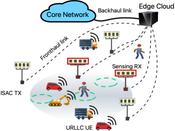
Figure 1: Illustration of the ISAC system in cell-free massive MIMO with URLLC UEs.

Concurrently, the $N_{\rm rx}$ sensing receive APs engage in simultaneous sensing of the candidate location to detect the target. Each AP is equipped with an array of $M$ antennas configured in a horizontal uniform linear array (ULA) with half-wavelength spacing. The respective array response vector is $\textbf{a}(\varphi,\vartheta)=\begin{bmatrix}1\!&\!e^{j\pi\sin(\varphi)\cos(\vartheta)}&\ldots&e^{j(M-1)\pi\sin(\varphi)\cos(\vartheta)}\end{bmatrix}^{T},$ where $\varphi$ and $\vartheta$ are the azimuth and elevation angles from the AP to the target location, respectively [28].

We consider the finite blocklength regime for URLLC UEs, where a packet of $b_{i}$ bits is sent to UE $i$ within a transmission block with blocklength $L=L_{p}+L_{d}$ symbols using the coherence bandwidth $B$. $L_{p}$ and $L_{d}$ are the number of symbols for pilot and data, respectively. It is expected that duration of each URLLC transmission, denoted by $T$, is shorter than one coherence time $T_{c}$, i.e., $T<T_{c}$ [17]. Without loss of generality, we assume the coherence time is equal to URLLC transmission time so that in for each transmission we first estimate the channel.

II-A Channel Modeling and Downlink Communications

The communication channels are modeled as spatially correlated Rician fading which are assumed to remain constant during each coherence block, and the channel realizations are independent of each other. Let $\textbf{h}_{i,k}\in\mathbb{C}^{M}$ denote the channel between ISAC AP $k$ and UE $i$, modeled as

$$\textbf{h}_{i,k}=e^{j\varphi_{i,k}}\bar{\textbf{h}}_{i,k}\,+\,\tilde{\textbf{h}}_{i,k},$$ (1)

which consists of a semi-deterministic line-of-sight (LOS) path, represented by $e^{j\varphi_{i,k}}\bar{\textbf{h}}_{i,k}$ with unknown phase-shift $\varphi_{i,k}\sim\mathcal{U}[0,2\pi)$, i.e., uniformly distributed on $[0,2\pi)$, and a stochastic non-LOS (NLOS) component $\tilde{\textbf{h}}_{i,k}\sim\mathcal{CN}(\textbf{0},\textbf{R}_{i,k})$ with the spatial correlation matrix $\textbf{R}_{i,k}\in\mathbb{C}^{M\times M}$. Both $\bar{\textbf{h}}_{i,k}$ and $\textbf{R}_{i,k}$ include the combined effect of geometric path loss and shadowing. We concatenate the channel vector $\textbf{h}_{i,k}$ in the collective channel vector

$$\textbf{h}_{i}=\begin{bmatrix}\textbf{h}_{i,1}^{T}&\ldots&\textbf{h}_{i,N_{\rm tx}}^{T}\end{bmatrix}^{T}\in\mathbb{C}^{N_{\rm tx}M}$$ (2)

for UE $i$.

Let $s_{i}[m]$ and $s_{0}[m]$ represent the downlink communication symbol for UE $i$ and sensing symbol, respectively at time instance $m$. The symbols are independent and have zero mean and unit power. Moreover, let $\rho_{i}\geq 0$ and $\rho_{0}\geq 0$ be, respectively, the power control coefficients for UE $i$ and the target, which are fixed throughout the transmission. Then, the transmitted signal from transmit AP $k\in\{1,\cdots,N_{\rm tx}\}$ at time instance $m$ is

$$\vspace{-1mm}\textbf{x}_{k}[m]=\sum_{i=0}^{N_{\rm ue}}\sqrt{\rho_{i}}\textbf{w}_{i,k}s_{i}[m]=\textbf{W}_{k}\textbf{D}_{\rm s}[m]\boldsymbol{\rho},\vspace{-1mm}$$ (3)

where the vectors $\textbf{w}_{i,k}\in\mathbb{C}^{M}$ and $\textbf{w}_{0,k}\in\mathbb{C}^{M}$ are the transmit precoding vectors for transmit AP $k$ corresponding to UE $i$ and the sensing signal, respectively. In (3), $\textbf{W}_{k}=\begin{bmatrix}\textbf{w}_{0,k}&\textbf{w}_{1,k}&\cdots&\textbf{w}_{N_{\rm ue},k}\end{bmatrix}$, ${\textbf{D}}_{\rm s}[m]=\textrm{diag}\left(s_{0}[m],s_{1}[m],\ldots,s_{N_{\rm ue}}[m]\right)$ is the diagonal matrix containing the sensing and communication symbols, and $\boldsymbol{\rho}=[\sqrt{\rho_{0}}\ \ldots\ \sqrt{\rho_{N_{\rm ue}}}]^{T}$.

Moreover, let $n_{i}[m]\!\sim\!\mathcal{CN}(0,\sigma_{n}^{2})$ be the independent receiver noise at UE $i$ at time instance $m$. The received signal at UE $i$ is given as

$$y_{i}[m]= \underbrace{\sqrt{\rho_{i}}\textbf{h}_{i}^{H}\textbf{w}_{i}s_{i}[m]}_{\textrm{Desired signal}}+\underbrace{\sum_{j=1,j\neq i}^{N_{\rm ue}}\sqrt{\rho_{j}}\textbf{h}_{i}^{H}\textbf{w}_{j}s_{j}[m]}_{\textrm{Interference signal due to the other UEs}}$$

$$+\underbrace{\sqrt{\rho_{0}}\textbf{h}_{i}^{H}\textbf{w}_{0}s_{0}[m]}_{\textrm{Interference signal due to the sensing}}+\underbrace{n_{i}[m]}_{\textrm{Noise}},$$ (4)

where the collective precoding vectors

$${\textbf{w}_{i}=\left[\textbf{w}_{i,1}^{T}\ \textbf{w}_{i,2}^{T}\ \ldots\ \textbf{w}_{i,N_{\rm tx}}^{T}\right]^{T}\in\mathbb{C}^{N_{\rm tx}M}},$$ (5)

for $i=1,\ldots,N_{\rm ue}$, and

$$\textbf{w}_{0}=\left[\textbf{w}_{0,1}^{T}\ \textbf{w}_{0,2}^{T}\ \ldots\ \textbf{w}_{0,N_{\rm tx}}^{T}\right]^{T}\in\mathbb{C}^{N_{\rm tx}M},$$ (6)

are the centralized precoding vectors. The vectors $\textbf{w}_{i,k}\in\mathbb{C}^{M}$ and $\textbf{w}_{0,k}\in\mathbb{C}^{M}$ are the transmit precoding vectors for ISAC AP $k$ corresponding to UE $i$ and the sensing signal, respectively.

Using the independence of the data and sensing signals, the average transmit power for transmit AP $k\in\{1,\ldots,N_{\rm tx}\}$ is

$$P_{k}=\sum_{i=0}^{N_{\rm ue}}\rho_{i}\mathbb{E}\left\{\|\textbf{w}_{i,k}\|^{2}\right\},\quad k=1,\ldots,N_{\rm tx}$$ (7)

which should not exceed the maximum power limit $P_{\rm tx}$.

In the subsequent section, we will present the specifics of the linear minimum mean-squared error (LMMSE)-based channel estimation.

II-B LMMSE-Based Channel Estimation

Within the URLLC transmission time comprising $L$ symbols, $L_{p}<L$ symbols are allocated for pilot transmission. A collection of $L_{p}$ mutually orthogonal pilot sequences is represented by $\boldsymbol{\phi}_{1},\ldots,\boldsymbol{\phi}_{L_{p}}\in\mathbb{C}^{L_{p}}$, where $\|\boldsymbol{\phi}_{t}\|^{2}=L_{p}$ for $t=1,\ldots,L_{p}$. These pilot sequences are assigned to the $N_{\rm ue}$ UEs. If the number of pilot sequences is less than the number of UEs (i.e., $L_{p}<N_{\rm ue}$), then each pilot sequence may be assigned to multiple UEs. Let $t_{i}\in\{1,\ldots,L_{p}\}$ denote the index of the pilot sequence that is assigned to UE $i$ and we define $\mathcal{P}_{i}=\{j\in\{1,\ldots,N_{\rm ue}\}|t_{j}=t_{i}\}$ as the set of UEs that share the same pilot with UE $i$.

The received signal at the ISAC AP $k$ during the entire pilot transmission is denoted by $\textbf{Y}_{k}^{p}\in\mathbb{C}^{M\times L_{p}}$ where

$$\textbf{Y}_{k}^{p}=\sum_{i=1}^{N_{\rm ue}}\sqrt{\eta_{i}}\textbf{h}_{i,k}\boldsymbol{\phi}_{t_{i}}^{T}+\textbf{N}_{k},$$ (8)

where $\eta_{i}>0$ is the transmit power by UE $i$ and $\textbf{N}_{k}\in\mathbb{C}^{M\times L_{p}}$ is the received noise at AP $k$ with independent and identically distributed (i.i.d.) $\mathcal{CN}(0,\sigma_{n}^{2})$ entries. We assume that $\bar{\textbf{h}}_{i,k}$ and $\textbf{R}_{i,k}$, representing the long-term statistics for the channel in (1), are known while the random phase-shift $\varphi_{i,k}$ is unknown. With respect to estimating $\textbf{h}_{i,k}$, let us form $\textbf{y}_{t_{i},k}^{p}=\frac{1}{\sqrt{L_{p}}}\textbf{Y}_{k}^{p}\boldsymbol{\phi}_{t_{i}}^{*}\in\mathbb{C}^{M}$, where

$$\textbf{y}_{t_{i},k}^{p}=\underbrace{\sqrt{\eta_{i}L_{p}}\textbf{h}_{i,k}}_{\textrm{Desired part}}+\underbrace{\sum_{j\in\mathcal{P}_{i}\setminus\{i\}}\sqrt{\eta_{j}L_{p}}\textbf{h}_{j,k}}_{\textrm{Interference part}}+\underbrace{\textbf{n}_{t_{i},k}}_{\textrm{Noise}},$$ (9)

where $\textbf{n}_{t_{i},k}=\frac{1}{\sqrt{L_{p}}}\textbf{N}_{k}\boldsymbol{\phi}_{t_{i}}^{*}\sim\mathcal{CN}(\textbf{0},\sigma_{n}^{2}\textbf{I}_{M})$. If the number of UEs is greater than the number of mutually orthogonal pilot sequences, then each pilot sequence may be assigned to multiple UEs using the pilot assignment algorithm in [27, Alg. 4.1]. The LMMSE estimate of $\textbf{h}_{i,k}$ is given by [29]

$$\hat{\textbf{h}}_{i,k}=\sqrt{\eta_{i}L_{p}}\textbf{R}_{i,k}^{\prime}\left(\boldsymbol{\Psi}^{\prime}_{t_{i},k}\right)^{-1}\textbf{y}_{t_{i},k}^{p},$$ (10)

where $\textbf{R}_{i,k}^{\prime}$ and $\boldsymbol{\Psi}_{t_{i},k}^{\prime}$ are the spatial correlation matrix corresponding to channel $\textbf{h}_{i,k}$ and the correlation matrix of the received signal, respectively, given by

$$\textbf{R}_{i,k}^{\prime}\triangleq\textbf{R}_{i,k}+\bar{\textbf{h}}_{i,k}\bar{\textbf{h}}_{i,k}^{H}$$ (11)

$$\boldsymbol{\Psi}^{\prime}_{t_{i},k}\triangleq\sum_{j\in\mathcal{P}_{i}}\eta_{j}L_{p}\textbf{R}_{j,k}^{\prime}+\sigma_{n}^{2}\textbf{I}_{M}.$$ (12)

It is worth noting that deriving MMSE channel estimation proves challenging due to the non-Gaussian distribution of channels resulting from random phase-shifts in the LOS paths. For the sake of tractability, we adhere to the use of LMMSE-based channel estimation in this paper.

II-C Multi-Static Sensing

We investigate multi-static sensing, involving multiple transmit and receive APs in the network. The network engages in target location sensing during the downlink phase. We assume the existence of a LOS connection between the target location and each transmit/receive AP.

In the presence of the target, each receive AP captures both the reflected signals from the target and undesired signals, referred to as clutter. The clutter, being independent of the target’s presence, is treated as interference for sensing purposes. Without loss of generality, we assume that the LOS paths between transmit and receive APs are known and can be effectively canceled out. Consequently, the interference signals correspond to the reflected paths through obstacles and are henceforth denoted as target-free channels.

Let $\textbf{H}_{r,k}\in\mathbb{C}^{M\times M}$ denote the target-free channel matrix between transmit AP $k$ and receive AP $r$. We use the correlated Rayleigh fading model for the NLOS channels $\textbf{H}_{r,k}$, which is modeled using the Kronecker model [30]. We define the random matrix $\textbf{W}_{{\rm ch},(r,k)}\in\mathbb{C}^{M\times M}$ with i.i.d. entries with $\mathcal{CN}(0,1)$ distribution. The matrix $\textbf{R}_{{\rm rx},(r,k)}\in\mathbb{C}^{M\times M}$ represents the spatial correlation matrix corresponding to receive AP $r$ and with respect to the direction of transmit AP $k$. Similarly, $\textbf{R}_{{\rm tx},(r,k)}\in\mathbb{C}^{M\times M}$ is the spatial correlation matrix corresponding to transmit AP $k$ and with respect to the direction of receive AP $r$. The channel $\textbf{H}_{r,k}$ is written as

$$\textbf{H}_{r,k}=\textbf{R}^{\frac{1}{2}}_{{\rm rx},(r,k)}\textbf{W}_{{\rm ch},{(r,k)}}\left(\textbf{R}^{\frac{1}{2}}_{{\rm tx},(r,k)}\right)^{T},$$ (13)

where the channel gain is determined by the geometric path loss and shadowing, and is included in the spatial correlation matrices. The received signal at AP $r$ in the presence of the target and for $m\in\{1,\cdots,L_{d}\}$, can be formulated as

$$\textbf{y}_{r}[m]=\sum_{k=1}^{N_{\rm tx}}\underbrace{\alpha_{r,k}\sqrt{\beta_{r,k}}\textbf{a}(\phi_{r},\theta_{r})\textbf{a}^{T}(\varphi_{k},\vartheta_{k})\textbf{x}_{k}[m]}_{\textrm{desired reflections from the target}}$$

$$+\sum_{k=1}^{N_{\rm tx}}\underbrace{\textbf{H}_{r,k}\textbf{x}_{k}[m]}_{\textrm{undesired signals}}+\textbf{n}_{r}[m],$$ (14)

where $\textbf{n}_{r}[m]\sim\mathcal{CN}(\textbf{0},\sigma_{n}^{2}\textbf{I}_{M})$ is the receiver noise at the $M$ antennas of receive AP $r$. The second term in (II-C) acts as interference for the target detection. Here, $\beta_{r,k}$ is the channel gain including the path-loss from transmit AP $k$ to receive AP $r$ through the target and the variance of bi-static radar cross-section (RCS) of the target denoted by $\sigma_{\rm rcs}$. The $\alpha_{r,k}\!\sim\!\mathcal{CN}(0,\,1)$ is the normalized RCS of the target for the respective path. We assume the RCS values are i.i.d. and follow the Swerling-I model, meaning that they are constant throughout the consecutive $L_{d}$ symbols collected for sensing [26].

Following the same notation as in [25], in (II-C), the known part of each reflected path is denoted by ${\textbf{g}_{r,k}[m]\in\mathbb{C}^{M}}$, defined as

$$\textbf{g}_{r,k}[m]\triangleq\sqrt{\beta_{r,k}}\textbf{a}(\phi_{r},\theta_{r})\textbf{a}^{T}(\varphi_{k},\vartheta_{k})\textbf{x}_{k}[m],$$ (15)

where the matrix $\alpha_{r,k}\sqrt{\beta_{r,k}}\textbf{a}(\phi_{r},\theta_{r})\textbf{a}^{T}(\varphi_{k},\vartheta_{k})$ represents the reflected path through the target. Here, $\phi_{r}$ and $\theta_{r}$ denote the azimuth and elevation angles from the target location to receiver AP $r$, respectively. Similarly, $\varphi_{k}$ and $\vartheta_{k}$ represent the azimuth and elevation angles from transmit AP $k$ to the target location.

Each receive AP sends their respective signals $\textbf{y}_{r}[m]$, for $r=1,\ldots,N_{\rm rx}$, to the edge cloud, to form the collective received signal $\textbf{y}[m]=\begin{bmatrix}\textbf{y}_{1}^{T}[m]&\cdots&\textbf{y}_{N_{\rm rx}}^{T}[m]\end{bmatrix}^{T}$, which can be expressed as

$$\textbf{y}[m] =\underbrace{\mathrm{blkdiag}\left(\textbf{G}_{1}[m],\ldots,\textbf{G}_{N_{\rm rx}}[m]\right)}_{\triangleq\textbf{G}[m]}\boldsymbol{\alpha}$$

$$+\underbrace{\left(\textbf{I}_{N_{\rm rx}}\otimes\left(\textbf{x}^{T}[m]\otimes\textbf{I}_{M}\right)\right)}_{\triangleq\textbf{X}[m]}\boldsymbol{\mathfrak{h}}+\textbf{n}[m],$$ (16)

where $\textbf{G}_{r}[m]=\begin{bmatrix}\textbf{g}_{r,1}[m]&\cdots&\textbf{g}_{r,N_{\rm tx}}[m]\end{bmatrix}\in\mathbb{C}^{M\times N_{\rm tx}}$, $\textbf{x}[m]=\begin{bmatrix}\textbf{x}^{T}_{1}[m]&\cdots&\textbf{x}^{T}_{N_{\rm tx}}[m]\end{bmatrix}^{T}\in\mathbb{C}^{N_{\rm tx}M}$, and $\mathfrak{h}\sim\mathcal{CN}\left(\textbf{0},\textbf{R}\right)$ is the vectorized target-free channels[25, Sec. V].

II-D Transmit ISAC Precoding Vectors

The communication and sensing transmit precoding vectors are obtained based on regularized zero forcing (RZF) and zero forcing (ZF) approaches, respectively. The unit-norm RZF precoding vector for UE $i$ is given as $\textbf{w}_{i}=\frac{\bar{\textbf{w}}_{i}}{\left\|\bar{\textbf{w}}_{i}\right\|}$, with

$$\bar{\textbf{w}}_{i}\!=\!\left(\sum\limits_{j=1}^{N_{\rm ue}}\hat{\textbf{h}}_{j}\hat{\textbf{h}}_{j}^{H}+\delta\textbf{I}_{N_{\rm tx}M}\right)^{\!\!-1}\!\!\hat{\textbf{h}}_{i},\quad i=1,\ldots,N_{\rm ue},$$ (17)

where $\delta$ is the regularization parameter, and $\hat{\textbf{h}}_{j}=\begin{bmatrix}\hat{\textbf{h}}_{j,1}^{T}&\ldots&\hat{\textbf{h}}_{j,N_{\rm tx}}^{T}\end{bmatrix}^{T}\in\mathbb{C}^{N_{\rm tx}M}$ is the LMMSE channel estimate of the communication channel $\textbf{h}_{j}$.

We aim to null the destructive interference from the sensing signal to the UEs by using the unit-norm ZF sensing precoding vector $\textbf{w}_{0}=\frac{\bar{\textbf{w}}_{0}}{\left\|\bar{\textbf{w}}_{0}\right\|}$, where

$$\bar{\textbf{w}}_{0}=\left(\textbf{I}_{N_{\rm tx}M}-\textbf{U}\textbf{U}^{H}\right)\textbf{h}_{0},$$ (18)

and U is the unitary matrix with the orthogonal columns that span the column space of the matrix $\begin{bmatrix}\hat{\textbf{h}}_{1}&\ldots&\hat{\textbf{h}}_{N_{\rm ue}}\end{bmatrix}$. $\textbf{h}_{0}=\begin{bmatrix}\sqrt{\beta_{1}}\textbf{a}^{T}(\varphi_{1},\vartheta_{1})&\ldots&\sqrt{\beta_{N_{\rm tx}}}\textbf{a}^{T}(\varphi_{N_{\rm tx}},\vartheta_{N_{\rm tx}})\end{bmatrix}^{T}\in\mathbb{C}^{N_{\rm tx}M}$ is the concatenated sensing channel between all the ISAC APs and the target, including corresponding path loss and the array response vectors $\textbf{a}(\varphi_{k},\vartheta_{k})$ for $k=1,\ldots,N_{\rm tx}$.

III Reliability and Delay Analysis for URLLC

In this section, we derive an upper bound on the DEP and the transmission delay, both crucial aspects considered as URLLC requirements. In the finite blocklength regime, the communication data cannot be transmitted without error. From [16], ergodic data rate of UE $i$ can be approximated as

$$R_{i}\!\approx\!\mathbb{E}\Bigg{\{}\!\!\left(1\!-\!\beta\right)\!\log_{2}{\left(1+\mathsf{SINR}^{\rm(dl)}_{i}\right)}\!-\!\frac{Q^{-1}(\epsilon_{i})}{\ln(2)}\!\sqrt{\!\frac{(1\!-\!\beta)V_{i}}{L}}\Bigg{\}},\vspace{-0mm}$$ (19)

where $\beta=\frac{L_{p}}{L}$, $\epsilon_{i}$ denotes the DEP when transmitting $b_{i}$ bits to UE $i$, $\mathsf{SINR}^{\rm(dl)}_{i}$ is the instantaneous downlink communication signal-to-interference-plus-noise ratio (SINR) for UE $i$, $V_{i}=1-\left(1+\mathsf{SINR}^{\rm(dl)}_{i}\right)^{-2}$ is the channel dispersion, and $Q(\cdot)$ refers to the Gaussian Q-function. Due to the fact that $V_{i}<1$, the ergodic data rate can be lower bounded by

$$R_{i} \!\geq\!\left(1\!-\!\beta\right)\!\mathbb{E}\Bigg{\{}\!\!\log_{2}{\left(1+\mathsf{SINR}^{(\rm dl)}_{i}\right)}\!\!\Bigg{\}}\!-\!\frac{Q^{-1}(\epsilon_{i})}{\ln(2)}\sqrt{\frac{(1-\beta)}{L}}.$$ (20)

Moreover, given that only $\mathbb{E}\left\{\textbf{h}_{i}^{H}\textbf{w}_{i}\right\}$ is known at UE $i$, and according to [27, Thm. 6.1] and [25, Lem. 1],

$$\mathbb{E}\left\{\log_{2}{\left(1+\mathsf{SINR}^{\rm(dl)}_{i}\right)}\right\}\geq\log_{2}{\left(1+\overline{\mathsf{SINR}}^{(\rm dl)}_{i}\right)}$$ (21)

where

$$\overline{\mathsf{SINR}}^{(\rm dl)}_{i}=\frac{\rho_{i}\mathsf{b}_{i}^{2}}{\sum_{j=0}^{{\rm N_{ue}}}\rho_{j}\mathsf{a}_{i,j}^{2}+\sigma_{n}^{2}},\quad i=1,\ldots,N_{\rm ue}$$ (22)

with

$$\mathsf{b}_{i}=\left|\mathbb{E}\left\{\textbf{h}_{i}^{H}\textbf{w}_{i}\right\}\right|,\quad\mathsf{a}_{i,i}=\sqrt{\mathbb{E}\left\{\left|\textbf{h}_{i}^{H}\textbf{w}_{i}\right|^{2}\right\}-\mathsf{b}_{i}^{2}}$$ (23)

$$\mathsf{a}_{i,j}=\sqrt{\mathbb{E}\left\{\left|\textbf{h}_{i}^{H}\textbf{w}_{j}\right|^{2}\right\}},\quad j=0,1,\ldots,N_{\rm ue},\quad j\neq i.$$ (24)

The expectations are taken with respect to the random channel realizations. Now, using (21) and substituting $R_{i}=\frac{b_{i}}{L}$ into (20), we obtain an upper bound for the DEP as

$$\epsilon_{i}\leq\epsilon_{i}^{\rm(ub)}\!\triangleq\!Q\!\left(\sqrt{L-L_{p}}\left[\ln\left(1+\overline{\mathsf{SINR}}^{(\rm dl)}_{i}\right)-\frac{b_{i}\ln{2}}{L-L_{p}}\right]\right).$$ (25)

In this paper, we focus on the transmission delay and leave the analysis of E2E delay as future work. Let $D_{i}^{t}$ denote the transmission delay of UE $i$, expressed as

$$D_{i}^{\rm t}=\frac{T}{1-\epsilon_{i}}=\frac{L}{B(1-\epsilon_{i})},\quad i=1,\ldots,N_{\rm ue}$$ (26)

where $T=\frac{L}{B}$ is the time duration of one URLLC transmission with blocklength $L$. To satisfy the reliability requirement, $\epsilon_{i}$ should be less than the maximum tolerable DEP denoted by $\epsilon_{i}^{(\rm th)}$. Then, since $\epsilon_{i}\leq\epsilon_{i}^{\rm(ub)}\leq\epsilon_{i}^{\rm(th)}$, the transmission delay is upper-bounded as

$$D_{i}^{\rm t}\leq\frac{L}{B\left(1-\epsilon_{i}^{\rm(th)}\right)}\triangleq D_{i}^{\rm(ub)}\leq D_{i}^{\rm(th)},$$ (27)

where $D_{i}^{\rm(th)}$ is the maximum tolerable delay by UE $i$ and $D_{i}^{\rm(ub)}\leq D_{i}^{\rm(th)}$ should be satisfied to guarantee the delay requirement. This implies that the blocklength cannot exceed $D^{\rm(th)}_{i}B(1-\epsilon_{i}^{\rm(th)})$. Thus, we can define the maximum tolerable blocklength by $L_{\rm max}$, where

$$L_{\rm max}=\min\left\{D^{\rm(th)}_{i}B\left(1-\epsilon_{i}^{\rm(th)}\right)|i=1,\cdots,N_{\rm ue}\right\}.$$ (28)

IV Sensing Analysis

We have numerically shown in [19] and [25], that maximizing the sensing SINR improves the target detection probability under a constant false alarm probability. When studying other sensing tasks, it is naturally desired to keep the sensing SINR above a required threshold denoted by $\gamma_{\rm s}$, i.e., $\mathsf{SINR}_{s}\geq\gamma_{\rm s}$. This fact motivates the optimization problems presented in Section VI.

Using the previously defined vector $\boldsymbol{\rho}=[\sqrt{\rho_{0}}\ \ldots\ \sqrt{\rho_{N_{\rm ue}}}]^{T}$, from [25], the sensing SINR with independent RCS values is given by

$$\mathsf{SINR_{\rm s}}=\frac{\boldsymbol{\rho}^{T}\textbf{A}\boldsymbol{\rho}}{L_{d}MN_{\rm rx}\sigma_{n}^{2}+\boldsymbol{\rho}^{T}\textbf{B}\boldsymbol{\rho}},$$ (29)

where

$$\textbf{A}= M\,\sum_{m=1}^{L_{d}}\textbf{D}_{\rm s}^{H}[m]\Bigg{(}\sum_{r=1}^{N_{\rm rx}}\sum_{k=1}^{N_{\rm tx}}\beta_{r,k}\textbf{W}_{k}^{H}\textbf{a}^{*}(\varphi_{k},\vartheta_{k})\textbf{a}^{T}(\varphi_{k},\vartheta_{k})$$

$$\hskip 8.53581pt\times\textbf{W}_{k}\Bigg{)}\textbf{D}_{\rm s}[m],$$ (30)

B $$=\sum_{m=1}^{L_{d}}\textbf{D}_{\rm s}^{H}[m]\left(\sum_{r=1}^{N_{\rm rx}}\sum_{k=1}^{N_{\rm tx}}\mathrm{tr}\left(\textbf{R}_{\mathrm{rx},(r,k)}\right)\textbf{W}_{k}^{H}\textbf{R}^{T}_{{\rm tx},(r,k)}\textbf{W}_{k}\right)$$

$$\hskip 8.53581pt\times\textbf{D}_{\rm s}[m].$$ (31)

As we see, the sensing SINR is a function of symbols which are random for different blocklength values. When the blocklength is fixed, we can assume that the symbols are known in advance. This implies that although the symbols are known when processing the received sensing signals, they cannot be known during the resource allocation phase. To this end, we take the expectation with respect to the random symbols. Then, the average sensing SINR would be

$$\overline{\mathsf{SINR}}_{s} =\frac{\boldsymbol{\rho}^{T}\mathbb{E}\{\textbf{A}\}\boldsymbol{\rho}}{L_{d}MN_{\rm rx}\sigma_{n}^{2}+\boldsymbol{\rho}^{T}\mathbb{E}\{\textbf{B}\}\boldsymbol{\rho}},$$ (32)

The symbols $s_{i}[m]$ are independent, having zero mean and unit variance. Therefore, $\mathbb{E}\{s_{i}^{*}[m]s_{i}[m]\}=1$ and $\mathbb{E}\{s_{i}^{*}[m]s_{j}[m]\}=0$ for $i\neq j$. Then, the expectations in (32) are obtained as follows

$$\mathbb{E}\{\textbf{A}\}=L_{d}\,M\textbf{A}_{D},\quad \mathbb{E}\{\textbf{B}\}=L_{d}\,\textbf{B}_{D},$$ (33)

where

$$\textbf{A}_{D}=\mathrm{diag}\Bigg{(}\mathrm{diag}\Bigg{(} \sum_{r=1}^{N_{\rm rx}}\sum_{k=1}^{N_{\rm tx}}\beta_{r,k}\textbf{W}_{k}^{H}\textbf{a}^{*}(\varphi_{k},\vartheta_{k})$$

$$\times\textbf{a}^{T}(\varphi_{k},\vartheta_{k})\textbf{W}_{k}\Bigg{)}\Bigg{)}$$ (34)

$$\textbf{B}_{D}=\mathrm{diag}\Bigg{(}\mathrm{diag}\Bigg{(} \sum_{r=1}^{N_{\rm rx}}\sum_{k=1}^{N_{\rm tx}}\mathrm{tr}\left(\textbf{R}_{\mathrm{rx},(r,k)}\right)\textbf{W}_{k}^{H}\textbf{R}^{T}_{{\rm tx},(r,k)}\textbf{W}_{k}\Bigg{)}\Bigg{)}.$$ (35)

The average sensing SINR with respect to symbols and RCS values is finally written as

$$\overline{\mathsf{SINR}}_{s} =\frac{M\boldsymbol{\rho}^{T}\textbf{A}_{D}\boldsymbol{\rho}}{MN_{\rm rx}\sigma_{n}^{2}+\boldsymbol{\rho}^{T}\textbf{B}_{D}\boldsymbol{\rho}}.$$ (36)

V E2E Power Consumption Modeling

Compared to communication networks, ISAC networks are expected to consume more power due to sensing tasks. In general, E2E power consumption in a system with C-RAN architecture is consisting of two main components: i) the radio site power consumption, including the AP power consumption and ii) the power consumption at the edge cloud, denoted by $P_{\rm cloud}$ [23].

In the considered C-RAN architecture, all processing is done in the cloud. Let $P_{\textrm{AP},0}^{\rm tx}$ and $P_{\textrm{AP},0}^{\rm rx}$ be the static power consumption of the transmit ISAC AP and the receive sensing AP, respectively. The total power consumption, taking into account both communication and sensing, can be expressed as

$$P_{\rm total} =\underbrace{\sum_{k=1}^{N_{\rm tx}}\left(P_{\textrm{AP},0}^{\rm tx}+\Delta^{\rm tr}P_{k}\right)+\sum_{r=1}^{N_{\rm rx}}P_{\textrm{AP},0}^{\rm rx}}_{\textrm{radio site power consumption}}+P_{\rm cloud}$$ (37)

where $\Delta^{\rm tr}$ is the slope of load-dependent transmission power consumption of each AP. The $P_{k}$ is the transmission power of the ISAC AP $k$ from (7). The power consumption at the cloud is modeled as

$$P_{\rm cloud} =P_{\rm fixed}+\frac{1}{\sigma_{\rm cool}}\Bigg{(}P_{\rm cloud,0}^{\rm proc}+\Delta_{\rm cloud}^{\rm proc}\frac{C_{\rm cloud}}{C_{\rm max}}\Bigg{)},$$ (38)

where $P_{\rm fixed}$ is the fixed power consumption at the cloud which is independent of the load. $P_{\rm cloud,0}^{\rm proc}$ is the processing power consumption in the idle mode. $\sigma_{\rm cool}\in(0,1]$ and $\Delta_{\rm cloud}^{\rm proc}$ denote the cooling efficiency of the cloud and the slope of the load-dependent power consumption for processing at the digital unit (DU) in the cloud, respectively. Moreover, $C_{\rm max}$ and $C_{\rm cloud}\in[0,C_{\rm max}]$ are the maximum processing capacity of the processing resources and the total processing resource utilization in giga-operations per second (GOPS), respectively[14, 31]. The processing resource utilization can be expressed as

$$C_{\rm cloud}=C_{\rm proc}^{\rm c}+C_{\rm proc}^{\rm s}$$ (39)

where $C_{\rm proc}^{\rm c}$ and $C_{\rm proc}^{\rm s}$ are the processing resource utilization due to communication and sensing tasks, respectively.

In the following parts, the required GOPS for communication and sensing in our system model is computed, respectively. We assess the computational complexity where only the numbers of real multiplications and divisions are counted. Each complex multiplication is equal to four real multiplications. We also consider memory overhead in arithmetic operation calculations by multiplying each operation by two as done in [32, 14]. Hence, each complex multiplication is counted as $4\cdot 2=8$ operations in computing the total GOPS.

V-A GOPS Analysis of Digital Operations for Communication at the Cloud

In this section, we analyze the GOPS for digital signal processing corresponding to the communication tasks including the uplink channel estimation and downlink transmission. To compute the number of real multiplications, we mainly follow the GOPS analysis in [28, App. B], [23].

Let $C_{\textrm{ch-est}}$ denote the computational complexity of the LMMSE channel estimation approach for all the APs. To compute the channel estimates, we first obtain the vectors $\textbf{y}_{t_{i},k}^{p}$. From [28, App. B], the multiplication of one matrix of size $M\times L_{p}$ with a vector of size $L_{p}\times 1$ results in $ML_{p}$ complex multiplications. Hence, obtaining $\textbf{y}_{t_{i},k}^{p}$ for $N_{\rm ue}$ UEs at all $N_{\rm tx}$ APs costs $8ML_{p}N_{\rm ue}N_{\rm tx}$ real multiplications/division in total, if $L_{p}\geq N_{\rm ue}$. Otherwise, the number of real multiplications/divisions would be $8ML_{p}^{2}N_{\rm tx}$. Moreover, we need to compute the matrices $\textbf{R}_{i,k}^{\prime}$ and $\boldsymbol{\Psi}_{t_{i},k}^{\prime}$, given that $\bar{\textbf{h}}_{i,k}$ and $\textbf{R}_{i,k}$ are known. However, this pre-computation can be neglected since the channel statistics are usually constant for a while and there is no need to compute them every coherence block. Finally, the multiplications in (10) costs $8M^{2}N_{\rm ue}N_{\rm tx}$ real operations. Then, $C_{\textrm{ch-est}}$ is equal to

$$C_{\textrm{ch-est}}=\left\{\begin{matrix}(8ML_{p}+8M^{2})N_{\rm ue}N_{\rm tx},&L_{p}\geq N_{\rm ue}\\ 8ML_{p}^{2}N_{\rm tx}+8M^{2}N_{\rm ue}N_{\rm tx},&L_{p}<N_{\rm ue}.&\end{matrix}\right.$$ (40)

The number of real multiplications/divisions to compute centralized RZF precoding vector for all the UEs from [28, App. B] is

$$C_{\textrm{prec-comp}} =\underbrace{\frac{8\left((MN_{\rm tx})^{2}+MN_{\rm tx}\right)}{2}N_{\rm ue}}_{\textrm{inside the parentheses}}$$

$$\quad+\underbrace{\frac{8\left((MN_{\rm tx})^{3}-MN_{\rm tx}\right)}{3}}_{\rm inversion}+N_{\rm ue}\cdot\underbrace{8(MN_{\rm tx})^{2}}_{\textrm{for}(.)^{-1}\hat{\textbf{h}}_{i}}$$

$$\quad+N_{\rm ue}\cdot\left(\underbrace{8MN_{\rm tx}}_{\textrm{computing }||\textbf{w}_{i}||}+\underbrace{4MN_{\rm tx}}_{\textrm{normalization}}\right)$$

$$=\left(12(MN_{\rm tx})^{2}+16MN_{\rm tx}\right)N_{\rm ue}$$

$$\quad+\frac{8\left((MN_{\rm tx})^{3}-MN_{\rm tx}\right)}{3}.$$ (41)

Reciprocity calibration and multiplication of the symbols by the precoding vectors, each costs $8L_{d}MN_{\rm ue}N_{\rm tx}$ real operations [33, 14]. Multiplying by the power coefficients also costs $4L_{d}MN_{\rm ue}N_{\rm tx}$. Finally, the GOPS corresponding to communication processing (i.e., channel estimation, precoding and reciprocity calibration) is computed as

$$C_{\textrm{proc}}^{\rm c}=\frac{B}{L10^{9}}\Bigg{(}C_{\textrm{ch-est}}+C_{\textrm{prec-comp}}+20L_{d}MN_{\rm ue}N_{\rm tx}\Bigg{)},$$ (42)

where we divided the total giga operations by the coherence time $L/B$.

V-B GOPS Analysis of Digital Operations for Sensing at the Cloud

In this subsection, we compute the GOPS for sensing operations. In downlink, first the sensing precoding vector $\textbf{w}_{0}$ should be obtained. Next operation is multiplying the sensing symbols by the sensing precoding vector and the sensing power coefficient which costs $12L_{d}MN_{\rm tx}$ real multiplications/divisions. Let $C_{\rm prec-comp}^{\rm s}$ be the number of real multiplications/divisions to compute the sensing precoder $\textbf{w}_{0}$. The unitary matrix U in (18) (subspace spanned by the UE channel estimation vectors) is already obtained when computing the RZF precoding vectors by matrix inversion and the corresponding $\mathbf{L}\mathbf{D}\mathbf{L}^{H}$ decomposition [28, Lem. B.2]. Therefore, the computational complexity of the ZF precoding vector $\textbf{w}_{0}$ is given by

$$C_{\rm prec-comp}^{\rm s} =8(MN_{\rm tx})^{2}+12MN_{\rm tx},$$ (43)

where the first term stands for matrix-vector multiplication and the second term corresponds to the cost of computing $||\textbf{w}_{0}||$ and normalization, which are counted as $8MN_{\rm tx}+4MN_{\rm tx}$.

After transmitting the signal in downlink, the reflected signals along with the interference signals are received at the receiver APs and sent to the cloud. At the cloud, these signals are processed for a specific sensing application. In this work we consider target detection and assess the number of real multiplications/divisions required to compute the test statistics. For target detection problems, we usually compute the test statistics and compare them with a threshold. The target is declared detected if the value of the test statistics is greater than the threshold. We assume that the threshold is constant. Therefore, we can neglect the computational complexity of obtaining the threshold. However, test statistics should be obtained for each transmission. We use the maximum a posteriori ratio test (MAPRT) detector proposed in [25, Lem. 2]. The test statistics is given by

$$T =\frac{1}{\sigma_{n}^{2}}\left(\begin{bmatrix}\textbf{a}^{H}&\textbf{b}^{H}\end{bmatrix}\left(\begin{bmatrix}\textbf{C}&\textbf{E}\\ \textbf{E}^{H}&\textbf{D}\end{bmatrix}^{-1}-\begin{bmatrix}\textbf{0}&\textbf{0}\\ \textbf{0}&\textbf{D}^{-1}\end{bmatrix}\right)\begin{bmatrix}\textbf{a}\\ \textbf{b}\end{bmatrix}\right),$$ (44)

where

$$\textbf{a}=\sum_{m=1}^{L_{d}}\textbf{G}^{H}[m]\textbf{y}[m],\quad\textbf{b}=\sum_{m=1}^{L_{d}}\textbf{X}^{H}[m]\textbf{y}[m],$$ (45)

$$\textbf{C}=\sum_{m=1}^{L_{d}}\textbf{G}^{H}[m]\textbf{G}[m]+\sigma_{n}^{2}\textbf{I}_{N_{\rm rx}N_{\rm tx}},$$ (46)

$$\textbf{D}=\sum_{m=1}^{L_{d}}\textbf{X}^{H}[m]\textbf{X}[m]+\sigma_{n}^{2}\textbf{R}^{-1},$$ (47)

$$\textbf{E}=\sum_{m=1}^{L_{d}}\textbf{G}^{H}[m]\textbf{X}[m].$$ (48)

Let $C_{\rm se-comp}$ denote the number of real multiplications/divisions to compute the test statistics $T$. The computational complexity can be expressed as

$$C_{\rm se-comp}=C_{\rm se-prep}+C_{\rm se-detector}$$ (49)

where $C_{\rm se-prep}$ and $C_{\rm se-detector}$ are the computational complexity of pre-processing and computing the test statistics for sensing, respectively. The former corresponds to computing (45)-(48), and the latter corresponds to computing the test statistics in (44). The computational complexity for pre-processing part and each step of computing the test statistics are listed in Table I. The total $C_{\rm se-prep}$ and $C_{\rm se-detector}$ are obtained as

$$C_{\rm se-prep}=L_{d}C_{{\rm se-prep},m}$$

$$L_{d}\Bigg{(}20MN_{\rm tx}N_{\rm rx}+16M^{2}N_{\rm tx}N_{\rm rx}+4N_{\rm rx}\left(N_{\rm tx}^{2}+N_{\rm tx}\right)M$$

$$\quad+4\left((MN_{\rm tx})^{2}+MN_{\rm tx}\right)+8N_{\rm rx}\,N_{\rm tx}^{2}\,M^{2}\Bigg{)}$$ (50)

$$C_{\rm se-detector}=8\frac{\left((1+M^{2})N_{\rm tx}N_{\rm rx}\right)^{3}-(1+M^{2})N_{\rm tx}N_{\rm rx}}{3}$$

$$\quad+8\frac{(M^{2}N_{\rm tx}N_{\rm rx})^{3}-M^{2}N_{\rm tx}N_{\rm rx}}{3}$$

$$\quad+8\,\left(\left((1+M^{2})N_{\rm tx}N_{\rm rx}\right)^{2}+(1+M^{2})N_{\rm tx}N_{\rm rx}\right),$$ (51)

where $C_{{\rm se-prep},m}$ is defined as $C_{\rm se-prep}/L_{d}$. Finally, the sensing GOPS is obtained as

$$C_{\rm proc}^{\rm s} =\frac{B}{L10^{9}}\Bigg{(}\underbrace{12L_{d}MN_{\rm tx}}_{\textrm{precoding + power}}+C_{\textrm{prec-comp}}^{\rm s}+\underbrace{C_{\rm se-comp}}_{\textrm{target detection}}\Bigg{)}.$$ (52)

TABLE I: Number of real multiplications/divisions for computing test statistics.

Operation	# of real multiplications/division
$\textbf{G}[m],\quad\forall m$	$20\,L_{d}\,MN_{\rm tx}N_{\rm rx}$
a	$8\,L_{d}\,M^{2}\,N_{\rm rx}\,N_{\rm tx}\,$
b	$8\,L_{d}\,M^{2}\,N_{\rm tx}\,N_{\rm rx}$
C	$4\,L_{d}N_{\rm rx}\left(N_{\rm tx}^{2}+N_{\rm tx}\right)M$
D	$4L_{d}\,\left((MN_{\rm tx})^{2}+MN_{\rm tx}\right)$
E	$8\,L_{d}\,N_{\rm rx}\,N_{\rm tx}^{2}\,M^{2}$
$\begin{bmatrix}\textbf{C}&\textbf{E}\\ \textbf{E}^{H}&\textbf{D}\end{bmatrix}^{-1}$	$8\frac{\left((1+M^{2})N_{\rm tx}N_{\rm rx}\right)^{3}-(1+M^{2})N_{\rm tx}N_{\rm rx}}{3}$
$\textbf{D}^{-1}$	$8\frac{(M^{2}N_{\rm tx}N_{\rm rx})^{3}-M^{2}N_{\rm tx}N_{\rm rx}}{3}$
$\begin{bmatrix}\textbf{a}^{H}&\textbf{b}^{H}\end{bmatrix}\begin{bmatrix}(.)&(.)\\ (.)&(.)\end{bmatrix}\begin{bmatrix}\textbf{a}\\ \textbf{b}\end{bmatrix}$	$8\,\left(\left((1+M^{2})N_{\rm tx}N_{\rm rx}\right)^{2}+(1+M^{2})N_{\rm tx}N_{\rm rx}\right)$

VI Joint blocklength and Power Optimization

In this paper, we aim to optimize the blocklength and the power control coefficients to minimize the energy consumption while URLLC and sensing requirements are satisfied. In the following subsections, we cast two non-convex optimization problems: i) minimizing only the energy consumption for transmission; ii) minimizing E2E energy consumption by taking into account the energy consumption at the radio site and the cloud.

VI-A Minimizing Energy Consumption for Transmission

The optimization problem can be cast as

$$\textbf{P1:}\quad\underset{\boldsymbol{\rho}\geq\textbf{0},L>L_{p}}{\textrm{minimize}}\quad E_{\rm tr}=\frac{L_{d}}{B}P_{\rm tr}\,$$ (53a)

subject to $$\epsilon_{i}\leq\epsilon^{\rm(ub)}_{i}\leq\epsilon^{\rm(th)}_{i},\quad\forall i>0$$ (53b)

$$L\leq L_{\rm max},\quad$$ (53c)

$$\overline{\mathsf{SINR}}_{s}\geq\gamma_{\rm s},\quad$$ (53d)

$$P_{k}\leq P_{\rm tx},\quad\quad\textrm{for}\quad k=1,\cdots,N_{\rm tx}$$ (53e)

$P_{\rm tr}=\sum_{k=1}^{N_{\rm tx}}P_{k}$ is the average power consumption for transmission, given as $P_{\rm tr}=\sum_{j=0}^{N_{\rm ue}}\rho_{j}=\|\boldsymbol{\rho}\|^{2}$, where $\boldsymbol{\rho}=[\sqrt{\rho_{0}}\ \ldots\ \sqrt{\rho_{N_{\rm ue}}}]^{T}$, due to the unit-power centralized precoding vectors. Constraints (53b) and (53c) correspond to the URLLC requirements. The $\gamma_{\rm s}$ is the required sensing SINR that is selected according to the target detection performance requirement and $P_{\rm tx}$ is the maximum transmit power per AP.

The aforementioned problem is challenging to solve due to its non-convex nature and the high coupling of variables. In the following theorem, we present an equivalent optimization problem by introducing newly defined auxiliary variables. This allows us to obtain a more tractable optimization problem.

Theorem 1.

Consider the problem in (53) and define the collective vectors $\textbf{r}=[r_{1}\ \ldots\ r_{N_{\rm ue}}]^{T}$ and $\boldsymbol{\chi}=[\chi_{1}\ \ldots\ \chi_{N_{\rm ue}}]^{T}$. The optimal solution $\{\boldsymbol{\rho}^{\star},L^{\star}\}$ of the problem given below is also an optimal solution to (53):

$$\underset{\boldsymbol{\rho},\boldsymbol{\chi},\textbf{r}\geq\textbf{0},L>L_{p},\bar{L}>0}{\textrm{minimize}}\quad\frac{\|\boldsymbol{\rho}\|^{2}}{\overline{L}}\,$$ (54a)

$$\textrm{subject to:}\,\quad L-L_{p}\leq\frac{1}{\overline{L}},$$ (54b)

$$\ln\left(1+\chi_{i}\right)-\chi_{i}+\frac{\rho_{i}\mathsf{b}_{i}^{2}}{r_{i}}\geq\frac{Q^{-1}\left(\epsilon_{i}^{\rm(th)}\right)}{\sqrt{L-L_{p}}}+\frac{b_{i}\ln{2}}{L-L_{p}}$$ (54c)

$$\left\|\begin{bmatrix}\sqrt{2}\mathsf{a}_{i,0}\sqrt{\rho_{0}}\\ \vdots\\ \sqrt{2}\mathsf{a}_{i,N_{\rm ue}}\sqrt{\rho_{N_{\rm ue}}}\\ \sqrt{2}\mathsf{b}_{i}\sqrt{\rho_{i}}\\ \sqrt{2}\sigma_{n}\\ 1+\chi_{i}\\ r_{i}\end{bmatrix}\!\right\|\leq 1+\chi_{i}+r_{i},\forall i,$$ (54d)

$$\boldsymbol{\rho}^{T}\left(\gamma_{\rm s}\textbf{B}_{D}-M\,\textbf{A}_{D}\,\right)\boldsymbol{\rho}\leq-\gamma_{\rm s}MN_{\rm rx}\sigma_{n}^{2}$$ (54e)

$$\left\|\textbf{F}_{k}\boldsymbol{\rho}\right\|\leq\sqrt{P_{\rm tx}},\quad k=1,\ldots,N_{\rm tx},$$ (54f)

$$L\leq L_{\rm max},\$$ (54g)

where ${\bf F}_{k}=\mathrm{diag}\left(\sqrt{\mathbb{E}\left\{\|{\bf w}_{0,k}\|^{2}\right\}},\ldots,\sqrt{\mathbb{E}\left\{\|{\bf w}_{N_{\rm ue},k}\|^{2}\right\}}\right)$.

Proof.

See Appendix A. ∎

The optimization problem in (54) is still not convex due to the non-convex constraints (54b), (54c) and (54e). The terms that destroy convexity are the convex terms $1/\overline{L}$ and $\frac{\rho_{i}\mathsf{b}_{i}^{2}}{r_{i}}$ (in terms of $\boldsymbol{\rho}$ and r) on the right-hand side of (54b) and the left-hand side of (54c), respectively. To this end, we apply the concave-convex procedure (CCP) approach to (54b) and (54c), and the FPP-SCA method [34] to (54e), wherein $-\boldsymbol{\rho}^{T}M\,\textbf{A}_{D}\boldsymbol{\rho}$ is a concave function. Moreover, to avoid any potential infeasibility issue regarding (54e) during the initial iterations of the algorithm, we add slack variable $\chi_{0}\geq 0$ and a slack penalty $\lambda$, to the convexified problem at the initial iterations. In subsequent iterations, we set $\chi_{0}$ to zero if it is less than a threshold, denoted as $\chi_{0}\leq\epsilon_{\chi}$. Finally, the convex problem that is solved at the $c^{\rm th}$ iteration becomes

$$\underset{\boldsymbol{\rho},\boldsymbol{\chi},\textbf{r}\geq\textbf{0},L,\bar{L}>L_{p},\chi_{0}\geq 0}{\textrm{minimize}}\quad\frac{\|\boldsymbol{\rho}\|^{2}}{\overline{L}}+\lambda\chi_{0}\,,$$ (55a)

$$\textrm{subject to}\quad{L-L_{p}}\leq\frac{2}{\overline{L}^{(c-1)}}-\frac{\overline{L}}{\left(\overline{L}^{(c-1)}\right)^{2}},$$ (55b)

$$\ln\left(1+\chi_{i}\right)-\chi_{i}+2\frac{\sqrt{\rho_{i}}^{(c-1)}\mathsf{b}_{i}^{2}\,\sqrt{\rho_{i}}}{r_{i}^{(c-1)}}-r_{i}\left(\frac{\sqrt{\rho_{i}}^{(c-1)}\mathsf{b}_{i}}{r_{i}^{(c-1)}}\right)^{2}$$

$$\hskip 14.22636pt\geq\frac{Q^{-1}\left(\epsilon_{i}^{\rm(th)}\right)}{\sqrt{L-L_{p}}}+\frac{b_{i}\ln{2}}{L-L_{p}}$$ (55c)

$$\gamma_{\rm s}\boldsymbol{\rho}^{T}\textbf{B}_{D}\boldsymbol{\rho}-2M\,\Re\left(\left(\boldsymbol{\rho}^{(c-1)}\right)^{T}\textbf{A}_{D}\boldsymbol{\rho}\right)$$

$$\hskip 14.22636pt\leq-\gamma_{\rm s}MN_{\rm rx}\sigma_{n}^{2}-M\left(\boldsymbol{\rho}^{(c-1)}\right)^{T}\textbf{A}_{D}\boldsymbol{\rho}^{(c-1)}+\chi_{0},$$ (55d)

$$\eqref{con3b},\eqref{con5b},\eqref{con6b}.$$

The steps of FPP-SCA and CCP procedure are outlined in Algorithm 1. We empirically observed that setting $\overline{L}^{(0)}=\frac{1}{L_{\rm max}-L_{p}}$, $\rho_{0}^{(0)}=0$ and $\sqrt{\rho_{i}}^{(0)}=10^{-3}\sqrt{P_{\rm tx}/N_{\rm ue}}$ for $i>0$ yields satisfactory results.

Algorithm 1 FPP-SCA and CCP Procedure for Problem (54).

1:Initialization: Set arbitrary $\boldsymbol{\rho}^{(0)},\textbf{r}^{(0)}\geq\textbf{0}$, the solution accuracy parameters $\epsilon,\epsilon_{\chi}>0$, $\overline{L}^{(0)}=\frac{1}{L_{\rm max}-L_{p}}$, and $\lambda>0$. Set the iteration counter to $c=0$, and a maximum iteration number $c_{\rm max}$. Moreover, let $\mathsf{F}^{(0)}=\infty$ be the initial value of objective function and $\Delta\mathsf{F}^{(c)}=\mathsf{F}^{(c)}-\mathsf{F}^{(c-1)}$ with $\mathsf{F}^{(-1)}=0$.

2:$c\leftarrow c+1$.

3:While $\Delta\mathsf{F}^{(c-1)}\geq\epsilon$ and $c\leq c_{\rm max}$, do

4:Set $\boldsymbol{\rho}^{(c)}$, $\overline{L}^{(c)}$, and $\textbf{r}^{(c)}$ to the solution of the convex problem in (55), where the previous iterates $\boldsymbol{\rho}^{(c-1)}$, $\overline{L}^{(c-1)}$, and $\textbf{r}^{(c-1)}$ are taken as constant.

5:If $\chi_{0}<\epsilon_{\chi}$, set $\chi_{0}=0$ for the next iteration.

6:End while

7:Output: The transmit power coefficients $\boldsymbol{\rho}^{(c)}$ and the blocklength $L^{(c)}$.

VI-B Minimizing E2E Energy Consumption

In this subsection, our objective is to minimize the E2E energy consumption. The optimization problem is formulated as follows

$$\textbf{P2:}\quad\underset{\boldsymbol{\rho}\geq\textbf{0},L>L_{p}}{\textrm{minimize}}\quad E_{\rm total}=\frac{L}{B}P_{\rm total}\,$$ (56a)

subject to $$\epsilon_{i}\leq\epsilon^{\rm(ub)}_{i}\leq\epsilon^{\rm(th)}_{i},\quad\forall i>0$$ (56b)

$$L\leq L_{\rm max},\quad$$ (56c)

$$\overline{\mathsf{SINR}}_{s}\geq\gamma_{\rm s},\quad$$ (56d)

$$P_{k}\leq P_{\rm tx},\quad\quad\textrm{for}\quad k=1,\cdots,N_{\rm tx}.$$ (56e)

The total power consumption can be rewritten as

$$P_{\rm total}=P_{\rm FIXED}+\Delta^{\rm tr}\|\boldsymbol{\rho}\|^{2}+\frac{1}{L}f_{1}+\frac{L_{d}}{L}f_{2}$$ (57)

where

$$P_{\rm FIXED}=\sum_{k=1}^{N_{\rm tx}}P_{\textrm{AP},0}^{\rm tx}+\sum_{r=1}^{N_{\rm rx}}P_{\textrm{AP},0}^{\rm rx}+P_{\rm fixed}+\frac{P_{\rm cloud,0}^{\rm proc}}{\sigma_{\rm cool}}$$ (58)

$$f_{1}=\frac{\Delta_{\rm cloud}^{\rm proc}}{\sigma_{\rm cool}C_{\rm max}}\frac{B}{10^{9}}\Bigg{(}C_{\textrm{ch-est}}+C_{\textrm{prec-comp}}+C_{\textrm{prec-comp}}^{\rm s}$$

$$\quad+C_{\rm se-detector}\Bigg{)}$$ (59)

$$f_{2}=\frac{\Delta_{\rm cloud}^{\rm proc}}{\sigma_{\rm cool}C_{\rm max}}\frac{B}{10^{9}}\left(20MN_{\rm ue}N_{\rm tx}+12MN_{\rm tx}+C_{{\rm se-prep},m}\right).$$ (60)

Similar to the approach of problem P1, we define a new variable $\bar{L}$ where $L-L_{p}\leq\frac{1}{\bar{L}}$. Then, the objective function (56a) is equivalent to

$$\mathsf{F_{2}}\triangleq\frac{1}{B}\left(L\left(P_{\rm FIXED}\right)+\left(L-L_{p}\right)f_{2}+\Delta^{\rm tr}\frac{\|\boldsymbol{\rho}\|^{2}}{\bar{L}}\right).$$ (61)

The non-convex optimization problem in (56) can be solved using the same approach in P1 as follows:

$$\underset{\boldsymbol{\rho},\boldsymbol{\chi},\textbf{r}\geq\textbf{0},L,\bar{L}>L_{p},\chi_{0}\geq 0}{\textrm{minimize}}\quad\mathsf{F_{2}}+\lambda\chi_{0},$$ (62a)

$$\textrm{subject to}\quad\eqref{con1c},\eqref{con2c},\eqref{con3c},\eqref{con3b},\eqref{con5b},\eqref{con6b}.$$

VII Numerical Results

In this section, we present numerical results to evaluate the performance of the proposed joint blocklength and power allocation algorithms. We consider a total area of 500 $\rm m\times$ 500 $\rm m$. The sensing location is in the center of the area, i.e., $(250,250)$. The number of antenna elements per AP is set to $M=4$. The $N_{\rm tx}=16$ ISAC transmit APs are uniformly distributed in the area. We consider the number of sensing receive APs equal to $N_{\rm rx}=1$ or $N_{\rm rx}=2$ where the first AP is located at $(200,250)$ and the second one is located at $(300,250)$. The total number of URLLC UEs in the network is $N_{\rm ue}=8$, unless otherwise stated. We set $P_{\rm tx}=100$ mW and the uplink pilot transmission power for each UE is $50$ mW.

The large-scale fading coefficients, shadowing parameters, probability of LOS, and the Rician factors are simulated based on the 3GPP Urban Microcell model, defined in [35, Table B.1.2.1-1, Table B.1.2.1-2, Table B.1.2.2.1-4]. The path losses for the Rayleigh fading target-free channels are also modeled by the 3GPP Urban Microcell model with the difference that the channel gains are multiplied by an additional scaling parameter equal to $0.3$ to suppress the known parts of the target-free channels due to LOS and permanent obstacles [25]. The sensing channel gains are computed by the bi-static radar range equation [26]. The carrier frequency, the bandwidth, and the noise variance are set to $1.9$ GHz, $200$ KHz, and $-114$ dBm, respectively. The number of pilot symbols is $L_{p}=10$.

TABLE II: Simulation Parameters

$\Delta^{\rm tr},\sigma_{\rm cool}$	4, 0.9	$P_{\rm fixed}$	120 W
$P_{\textrm{AP},0}^{\rm tx},P_{\textrm{AP},0}^{\rm rx}$	6.8$\cdot M$ W, 6.8$\cdot M$  W	$P_{\rm cloud,0}^{\rm proc}$	20.8 W
$\Delta_{\rm cloud}^{\rm proc}$	740 W	$C_{\rm max}$	1800 GOPS

The spatial correlation matrices for the communication channels are generated by using the local scattering model in [27, Sec. 2.5.3]. The RCS of the target is modeled by the Swerling-I model with $\sigma_{\rm rcs}=0\,\rm dBsm$. For all the UEs, we set the same packet size, the maximum transmission delay, and the DEP threshold to $b_{i}=256$ bits, $D_{i}^{\rm(th)}=1$ ms, and $\epsilon_{\rm th}=10^{-5}$, respectively unless otherwise stated. In the proposed algorithms, $\epsilon=10^{-3}$, $\epsilon_{\chi}=10^{-6}$, $\lambda=10$, and $c_{\rm max}=30$. The sensing SINR threshold is set to $\gamma_{s}=0$ dB, unless otherwise stated. The remaining parameters are detailed in Table II, where the values are consistent with those in [14], except for a scaling of the total processing capacity and the corresponding power of a DU by a factor of ten to accommodate all the processing in a single DU.

We compare the performance of two proposed algorithms: i) SeURLLC+, which aims to minimize the transmission energy consumption for as ISAC cell-free massive MIMO system with URLLC UEs, and ii) E2E SeURLLC+, which aims to minimize the E2E energy consumption. We also consider two baseline algorithms for only URLLC systems without integrating sensing: i) URLLC-only, and ii) E2E URLLC-only, which represent minimizing transmission energy and E2E energy, respectively.

Figure 2: E2E energy consumption over one transmission with different algorithms and with $N_{\rm rx}=1,2$.

In Fig. 2, we illustrate E2E energy consumption with varying algorithms and two values for the number of sensing receive APs. The chart breaks down energy consumption by system components and different operations, including transmission, ISAC APs, sensing receive APs, communication and sensing processing, and “Others” representing load-independent and idle mode power consumption at the cloud. It is shown that in URLLC-only scenarios, the majority of the energy consumption is related to the ISAC APs and then the load-independent and idle mode power consumption at the cloud. Remarkably, E2E energy minimization demonstrates a substantial reduction in energy consumption by approximately $50\%$ in URLLC-only scenarios. This underscores the importance of E2E energy-aware optimization. Conversely, in ISAC scenarios, the impact of E2E energy minimization is less pronounced, resulting in only a marginal decrease. However, we observe that the energy consumption due to sensing processing becomes predominant when $N_{\rm rx}=2$. This observation suggests a potential optimization avenue, as turning off one sensing receive AP can halve the energy consumption, contributing significantly to overall energy efficiency.

(a) E2E URLLC-only

(b) E2E SeURLLC+ , $N_{\rm rx}=1$

(c) E2E SeURLLC+ , $N_{\rm rx}=2$

Figure 3: Energy consumption in one transmission with a) E2E URLLC-only, b) E2E SeURLLC+ with $N_{\rm rx}=1$, and E2E SeURLLC+ with $N_{\rm rx}=2$.

To complete the findings in Fig. 2, we provide a comparative analysis of the energy consumption distribution across various components within the system in Fig. 3. E2E energy minimization algorithms are considered for a) URLLC-only scenario, b) ISAC scenario with 1 sensing receive AP, and c) ISAC scenario with 2 sensing receive APs. As shown in Fig. 3(a) and Fig. 3(b), the ISAC APs are the most energy consuming components. Notably, the increment in the number of sensing receive APs is accompanied by a significant rise in energy consumption corresponding to the processing of the received signals for target detection. This is evident that with the addition of another receive AP, the share of sensing processing increases up to $52\%$, approximately four times larger than the case with $N_{\rm rx}=1$.

Figure 4: Blocklength vs. decoding error probability threshold.

Figure 5: E2E energy consumption vs. decoding error probability threshold.

VII-A Impact of Reliability and Delay Requirements

In this subsection, we investigate the impact of the reliability and delay requirements on the performance of the above-mentioned algorithms. Fig. 4 shows the blocklength as a function of decoding error probability (DEP) threshold. Generally, the blocklength decreases by relaxing the reliability threshold in all the algorithms except URLLC-only. It is shown that the URLLC-only algorithm always ends up with the maximum available blocklength, i.e., $L_{\rm max}$, since increasing the blocklength allows lower transmit power to satisfy the reliability constraint. We also observe that minimizing only the transmission energy consumption will lead to higher blocklength values compared to the E2E energy minimization algorithms, i.e., E2E URLLC-only and E2E SeURLLC+. Compared to URLLC-only, the E2E URLLC-only algorithm results in a significant decrease in the blocklength to minimize the E2E energy consumption over one transmission. For ISAC scenarios, we see the same behaviours as in E2E URLLC-only. However, the blocklength is slightly higher due to the interplay between sensing power consumption and the blocklength as transmit power consumption will decrease with larger blocklength.

Fig. 5 illustrates the E2E energy consumption in terms of the DEP threshold. The results show that relaxing the reliability constraint would generally reduce the E2E energy consumption. However, ISAC scenarios demand higher energy consumption as it is expected. Moreover, we observe that algorithms that minimize E2E energy consumption outperform the corresponding algorithms which only minimize the transmission energy consumption. Particularly, when we do not integrate sensing in the system, there is a noticeable gap between performance of URLLC-only and E2E URLLC-only algorithms.

Figure 6: E2E energy consumption vs. maximum delay threshold.

The results for E2E energy consumption versus maximum delay threshold, $D_{i}^{(\rm tx)}$, are depicted in Fig. 6. As it is shown, E2E energy consumption does not change significantly with different maximum delay threshold, except for URLLC-only algorithm. The reason is that the URLLC-only algorithm would always result in the highest possible blocklength to minimize the transmission energy consumption while the optimized value for the blocklength with other algorithms would be much lower than the one with URLLC-only to minimize the energy consumption. That is why the SeURLLC+ has lower E2E energy consumption than URLLC-only. However, the results of E2E URLLC-only algorithm show that minimum E2E energy consumption could be archived by optimizing the blocklength with respect to E2E energy consumption. This behavior highlights the importance of the E2E energy minimization.

VII-B Impact of Sensing Requirement

Figure 7: Blocklength vs. sensing SINR threshold.

Figure 8: E2E energy consumption vs. sensing SINR threshold.

The impact of the sensing SINR threshold, $\gamma_{s}$, on the blocklength and E2E energy consumption is investigated in Fig. 7 and Fig. 8, respectively. E2E energy minimization leads to lower energy consumption as it is shown that E2E SeURLLC+ outperforms SeURLLC+. The reason can be found in Fig. 7. It is shown that E2E SeURLLC+ leads to lower blocklength which means lower E2E energy consumption. Moreover, we observe that the gap between the performance of these two algorithms gradually decreases by demanding higher sensing SINR threshold.

VIII Conclusion

In this paper, we proposed a joint blocklength and power control algorithm for a downlink cell-free massive MIMO system with multi-static sensing and URLLC users. We formulated two non-convex optimization problems, focusing on transmission energy minimization and E2E energy minimization, respectively. Numerical results demonstrated the superiority of the E2E energy minimization algorithm, particularly in scenarios with no sensing capability. Furthermore, our results revealed a growing significance of energy consumption related to sensing processing tasks with the increase in the number of sensing receive access points. This observation highlights a potential optimization avenue, as deactivating one sensing receive AP can effectively mitigate this dominance and contribute to overall energy efficiency. Furthermore, our findings indicated that a higher sensing SINR threshold leads to increased E2E energy consumption. This ultimately narrows the performance gap between the two proposed algorithms: the transmission-only approach and the E2E energy minimization approach.

Appendix A Proof of Theorem 1

Let us define a new optimization variable, denoted by $\overline{L}$, where $L-L_{p}\leq 1/\overline{L}$. Then, minimizing the objective function is equivalent to minimizing the following convex function (quadratic-over-linear function)

$$\frac{\|\boldsymbol{\rho}\|^{2}}{\overline{L}}\,.$$ (63)

Since the above function is minimized, at the optimal solution, it holds that $\overline{L}=1/L_{d}=1/(L-L_{p})$. According to (25), the reliability constraints in (53b) can be written in the form of

$$\ln\left(1+\frac{\rho_{i}\mathsf{b}_{i}^{2}}{\sum_{j=0}^{{\rm N_{ue}}}\rho_{j}\mathsf{a}_{i,j}^{2}+\sigma_{n}^{2}}\right)\!\geq\frac{Q^{-1}\left(\epsilon_{i}^{(\rm th)}\right)}{\sqrt{L-L_{p}}}+\frac{b_{i}\ln{2}}{L-L_{p}}$$ (64)

where $\overline{\mathsf{SINR}}^{\rm(dl)}_{i}$ is substituted by (22). To handle the non-convexity of the left-hand side in (64), we define a new variable $\chi_{i}$ and use fractional programming [36] to write the left-hand side as

$$\ln(1+\chi_{i})-\chi_{i}+(1+\chi_{i})\frac{\rho_{i}\mathsf{b}_{i}^{2}}{\sum_{j=0}^{{\rm N_{ue}}}\rho_{j}\mathsf{a}_{i,j}^{2}+\rho_{i}\mathsf{b}_{i}^{2}+\sigma_{n}^{2}}.$$ (65)

Moreover, to represent the upper bound to $\left(\sum_{j=0}^{{\rm N_{ue}}}\rho_{j}\mathsf{a}_{i,j}^{2}+\rho_{i}\mathsf{b}_{i}^{2}+\sigma_{n}^{2}\right)/(1+\chi_{i})$, we introduce the optimization variable $r_{i}$, similarly as in [14], for $i=1,\ldots,N_{\rm ue}$, where

$$\frac{\sum_{j=0}^{{\rm N_{ue}}}\rho_{j}\mathsf{a}_{i,j}^{2}+\rho_{i}\mathsf{b}_{i}^{2}+\sigma_{n}^{2}}{1+\chi_{i}}\leq r_{i},$$ (66)

which can be written as a second-order cone (SOC) constraint in (54d). We then re-cast the constraint in (65) as

$$\ln\left(1+\chi_{i}\right)-\chi_{i}+\frac{\rho_{i}\mathsf{b}_{i}^{2}}{r_{i}}\geq\frac{Q^{-1}\left(\epsilon_{i}^{\rm(th)}\right)}{\sqrt{L-L_{p}}}+\frac{b_{i}\ln{2}}{L-L_{p}}$$ (67)

which will not destroy optimality since we want to minimize $r_{i}$ to increase the left-hand side of the SINR constraint.

From (36), the sensing constraint in (53d) are expressed as

$$\boldsymbol{\rho}^{T}\left(\gamma_{\rm s}\textbf{B}_{D}-M\,\textbf{A}_{D}\,\right)\boldsymbol{\rho}\!\leq\!-\gamma_{\rm s}MN_{\rm rx}\sigma_{n}^{2}.$$ (68)

Finally, we define $\textbf{F}_{k}=\textrm{diag}\left(\sqrt{\mathbb{E}\left\{\|\textbf{w}_{0,k}\|^{2}\right\}},\ldots,\sqrt{\mathbb{E}\left\{\|\textbf{w}_{N_{\rm ue},k}\|^{2}\right\}}\right)$ and rewrite the per-AP power constraints in (53e) in SOC form in terms of $\boldsymbol{\rho}$ as $\left\|\textbf{F}_{k}\boldsymbol{\rho}\right\|\leq\sqrt{P_{\rm tx}},$ , for $k=1,\ldots,N_{\rm tx}$.

References

• [1] F. Liu, Y. Cui, C. Masouros, J. Xu, T. X. Han, Y. C. Eldar, and S. Buzzi, “Integrated sensing and communications: Towards dual-functional wireless networks for 6G and beyond,” IEEE J. Sel. Areas Commun., 2022.
• [2] W. Zhou, R. Zhang, G. Chen, and W. Wu, “Integrated sensing and communication waveform design: A survey,” IEEE Open J. Commun. Soc., vol. 3, pp. 1930–1949, 2022.
• [3] C. Ding, C. Zeng, C. Chang, J.-B. Wang, and M. Lin, “Joint precoding for MIMO radar and URLLC in ISAC systems,” in Proceedings of the 1st ACM MobiCom Workshop on Integrated Sensing and Communications Systems, 2022, pp. 12–18.
• [4] M. Ozger, M. Vondra, and C. Cavdar, “Towards beyond visual line of sight piloting of UAVs with ultra reliable low latency communication,” in 2018 IEEE Global Communications Conference (GLOBECOM), 2018, pp. 1–6.
• [5] C. Sun, C. She, C. Yang, T. Q. Quek, Y. Li, and B. Vucetic, “Optimizing resource allocation in the short blocklength regime for ultra-reliable and low-latency communications,” IEEE Trans. Wirel. Commun., vol. 18, no. 1, pp. 402–415, 2018.
• [6] A. Lancho, G. Durisi, and L. Sanguinetti, “Cell-free massive MIMO for URLLC: A finite-blocklength analysis,” IEEE Trans. Wirel. Commun., 2023.
• [7] F. Salehi, M. Ozger, and C. Cavdar, “Reliability and delay analysis of 3-dimensional networks with multi-connectivity: Satellite, HAPs, and cellular communications,” IEEE Transactions on Network and Service Management, pp. 1–1, 2023.
• [8] Q. Peng, H. Ren, C. Pan, N. Liu, and M. Elkashlan, “Resource allocation for cell-free massive MIMO-enabled URLLC downlink systems,” IEEE Transactions on Vehicular Technology, 2023.
• [9] J. Pritzker, J. Ward, and Y. C. Eldar, “Transmit precoder design approaches for dual-function radar-communication systems,” arXiv preprint arXiv:2203.09571, 2022.
• [10] R. Thomä, T. Dallmann, S. Jovanoska, P. Knott, and A. Schmeink, “Joint communication and radar sensing: An overview,” in EuCAP, 2021.
• [11] Y. Huang, Y. Fang, X. Li, and J. Xu, “Coordinated power control for network integrated sensing and communication,” IEEE Trans. Veh. Technol., 2022, to appear.
• [12] A. Zhang, M. L. Rahman, X. Huang, Y. J. Guo, S. Chen, and R. W. Heath, “Perceptive mobile networks: Cellular networks with radio vision via joint communication and radar sensing,” IEEE Veh. Technol. Mag., vol. 16, no. 2, pp. 20–30, 2020.
• [13] D. Wang, C. Zhang, Y. Du, J. Zhao, M. Jiang, and X. You, “Implementation of a cloud-based cell-free distributed massive mimo system,” IEEE Communications Magazine, vol. 58, no. 8, pp. 61–67, 2020.
• [14] Ö. T. Demir, M. Masoudi, E. Björnson, and C. Cavdar, “Cell-free massive MIMO in O-RAN: Energy-aware joint orchestration of cloud, fronthaul, and radio resources,” arXiv preprint arXiv:2301.06166, 2023.
• [15] X. Zhao and Y.-J. A. Zhang, “Joint beamforming and scheduling for integrated sensing and communication systems in URLLC,” in IEEE Glob. Commun. Conf., 2022, pp. 3611–3616.
• [16] H. Ren, C. Pan, Y. Deng, M. Elkashlan, and A. Nallanathan, “Joint pilot and payload power allocation for massive-MIMO-enabled URLLC IIoT networks,” IEEE J. Sel. Areas Commun., vol. 38, no. 5, pp. 816–830, 2020.
• [17] A. A. Nasir, H. D. Tuan, H. Q. Ngo, T. Q. Duong, and H. V. Poor, “Cell-free massive mimo in the short blocklength regime for URLLC,” IEEE Transactions on Wireless Communications, vol. 20, no. 9, pp. 5861–5871, 2021.
• [18] A. Sakhnini, M. Guenach, A. Bourdoux, H. Sahli, and S. Pollin, “A target detection analysis in cell-free massive mimo joint communication and radar systems,” in IEEE ICC, 2022, pp. 2567–2572.
• [19] Z. Behdad, Ö. T. Demir, K. W. Sung, E. Björnson, and C. Cavdar, “Power allocation for joint communication and sensing in cell-free massive MIMO,” in IEEE Glob. Commun. Conf., 2022, pp. 4081–4086.
• [20] Z. Behdad, Ö. T. Demir, K. W. Sung, and C. Cavdar, “Interplay between sensing and communication in cell-free massive MIMO with URLLC users,” submitted for a possible conference publication, 2023.
• [21] A. Alabbasi, X. Wang, and C. Cavdar, “Optimal processing allocation to minimize energy and bandwidth consumption in hybrid CRAN,” IEEE Transactions on Green Communications and Networking, vol. 2, no. 2, pp. 545–555, 2018.
• [22] M. Masoudi, Ö. T. Demir, J. Zander, and C. Cavdar, “Energy-optimal end-to-end network slicing in cloud-based architecture,” IEEE Open Journal of the Communications Society, vol. 3, pp. 574–592, 2022.
• [23] Ö. T. Demir, M. Masoudi, E. Björnson, and C. Cavdar, “Cell-free massive MIMO in virtualized CRAN: How to minimize the total network power?” in IEEE ICC, 2022.
• [24] Z. Yang, C. Pan, J. Hou, and M. Shikh-Bahaei, “Efficient resource allocation for mobile-edge computing networks with NOMA: Completion time and energy minimization,” IEEE Transactions on Communications, vol. 67, no. 11, pp. 7771–7784, 2019.
• [25] Z. Behdad, Ö. T. Demir, K. W. Sung, E. Björnson, and C. Cavdar, “Multi-static target detection and power allocation for integrated sensing and communication in cell-free massive MIMO,” arXiv preprint arXiv:2305.12523, 2023.
• [26] M. A. Richards, J. Scheer, and W. A. Holm, Principles of Modern Radar: Basic Principles.   New York, NY, USA: Scitech, 2010.
• [27] Ö. T. Demir, E. Björnson, and L. Sanguinetti, “Foundations of user-centric cell-free massive MIMO,” Found. Trends Signal Process., vol. 14, no. 3-4, pp. 162–472, 2021.
• [28] E. Björnson, J. Hoydis, and L. Sanguinetti, “Massive MIMO networks: Spectral, energy, and hardware efficiency,” Foundations and Trends® in Signal Processing, vol. 11, no. 3-4, pp. 154–655, 2017.
• [29] Z. Wang, J. Zhang, E. Björnson, and B. Ai, “Uplink performance of cell-free massive MIMO over spatially correlated Rician fading channels,” IEEE Communications Letters, vol. 25, no. 4, pp. 1348–1352, 2020.
• [30] D. Shiu, G. Foschini, M. Gans, and J. Kahn, “Fading correlation and its effect on the capacity of multielement antenna systems,” IEEE Trans. Commun., vol. 48, no. 3, pp. 502–513, 2000.
• [31] M. Masoudi, S. S. Lisi, and C. Cavdar, “Cost-effective migration toward virtualized C-RAN with scalable fronthaul design,” IEEE Systems Journal, vol. 14, no. 4, pp. 5100–5110, 2020.
• [32] C. Desset and B. Debaillie, “Massive MIMO for energy-efficient communications,” in 2016 46th European Microwave Conference (EuMC).   IEEE, 2016, pp. 138–141.
• [33] S. Malkowsky, J. Vieira, L. Liu, P. Harris, K. Nieman, N. Kundargi, I. C. Wong, F. Tufvesson, V. Öwall, and O. Edfors, “The world’s first real-time testbed for massive MIMO: Design, implementation, and validation,” IEEE Access, vol. 5, pp. 9073–9088, 2017.
• [34] O. Mehanna, K. Huang, B. Gopalakrishnan, A. Konar, and N. D. Sidiropoulos, “Feasible point pursuit and successive approximation of non-convex QCQPs,” IEEE Signal Process Lett., vol. 22, no. 7, pp. 804–808, 2014.
• [35] 3GPP, “Further advancements for E-UTRA physical layer aspects (release 9),” TS 36.814, 2017.
• [36] K. Shen and W. Yu, “Fractional programming for communication systems—part II: Uplink scheduling via matching,” IEEE Transactions on Signal Processing, vol. 66, no. 10, pp. 2631–2644, 2018.