A Hierarchical Framework with Spatio-Temporal Consistency Learning for Emergence Detection in Complex Adaptive Systems

Abstract

Emergence, a global property of complex adaptive systems (CASs) constituted by interactive agents, is prevalent in real-world dynamic systems, e.g., network-level traffic congestions. Detecting its formation and evaporation helps to monitor the state of a system, allowing to issue a warning signal for harmful emergent phenomena. Since there is no centralized controller of CAS, detecting emergence based on each agent’s local observation is desirable but challenging. Existing works are unable to capture emergence-related spatial patterns, and fail to model the nonlinear relationships among agents. This paper proposes a hierarchical framework with spatio-temporal consistency learning to solve these two problems by learning the system representation and agent representations, respectively. Especially, spatio-temporal encoders are tailored to capture agents’ nonlinear relationships and the system’s complex evolution. Representations of the agents and the system are learned by preserving the intrinsic spatio-temporal consistency in a self-supervised manner. Our method achieves more accurate detection than traditional methods and deep learning methods on three datasets with well-known yet hard-to-detect emergent behaviors. Notably, our hierarchical framework is generic, which can employ other deep learning methods for agent-level and system-level detection.

I Introduction

Many real-world dynamic systems can be regarded as complex adaptive systems (CASs) composed of autonomous, adaptive, and interacting agents, whose interactions at the micro level can result in emergent phenomena at the macro level, namely, emergence [1, 2, 3]. Figure 1(a) presents an example. When there is adequate space among cars, the road net enjoys a smooth traffic flow. When the distances between cars significantly narrow down, network-level congestion occurs as an emergent phenomenon. Emergence is irreducible to the properties of agents that constitute CAS, and it is unpredictable by nature [1, 4]. Nonetheless, it will be beneficial to detect the formation and evaporation of emergence, specifically, weak emergence that is scientifically relevant [5]. It can help monitor some global properties of the system and issue a warning signal when an undesirable phenomenon arrives. For example, reporting a traffic jam based on the feedback of cars can help with the health management of traffic systems. It will complement existing monitors relying on static devices like sensors or cameras [6].

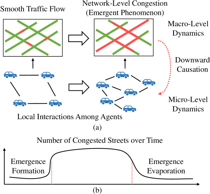
Figure 1: (a) Illustration of emergence. (b) Framing emergence detection as a change-point detection problem.

Emergence detection can be formulated as an online change-point detection (CPD) problem by regarding the time steps when emergence forms or evaporates as change points [7, 8]. As shown in Figure 1(b), the number of congested streets can serve as a global variable to monitor the emergence. However, CASs are distributed by nature, i.e., there is no centralized controller that can access the states of all agents. Therefore, methods requiring all agents’ states to compute a global metric for emergence detection become impractical under the distributed setting. Hence, it is desirable to detect emergence using agents’ local observation, which is feasible because all agents experience the downward causation [7] when the emergence forms, as shown in Figure 1(a). For example, cars slow down in a crowded street. Based on this observation, O’toole et al. [7] propose DETect, the only feasible emergence detection method for the distributed setting. In DETect, each agent analyzes its relationship with neighbors, communicates with them, and sends feedback when finding a noticeable change in the relationship. DETect concludes the formation or evaporation of emergence when the number of feedback gets significantly larger.

Though making a big step, DETect has two main limitations. First, it simply counts agents’ feedback to monitor the emergence, which may neglect the spatial patterns that are highly correlated to emergence. Second, it adopts linear regression to model an agent’s relationship with its neighbors, which may fail to capture nonlinear relationships.

This paper tries to overcome the above limitations from a graph perspective. CAS can be regarded as a dynamic graph [9], and thus emergence detection can be cast to online CPD in dynamic graphs under the distributed setting. Based on this formulation, it suffices to learn a system-level representation aware of emergence-related patterns, and agent-level representations encoding the nonlinear relationships. When emergence forms or evaporates, the system representations between adjacent time steps are expected to be inconsistent, which can serve as a detecting signal for emergence. Specifically, a Hierarchical framework with Spatio-Temporal Consistency Learning is proposed for Emergence Detection (HiSTCLED). HiSTGLED is of a three-layer structure, “agents-region monitors-global monitor”, which allows to capture emergence-related spatial patterns by aggregating agent-level detecting results from bottom-up. HiSTCLED can be conceptually implemented by the efficient end-edge-cloud collaborative framework. Spatio-temporal encoders (STEs) are designed to model the complex variation of agents’ nonlinear relationships and the system states on highly dynamic scenarios. The corresponding representations of agents and the system are learned by jointly preserving the spatial and temporal consistency through non-contrastive self-supervised learning strategies.

Our contributions are summarized as follows.

• The hierarchical framework HiSTCLED can capture emergence-related spatial patterns by aggregating agent-level detecting results from bottom-up.

• STEs are tailored to model the nonlinear relationships among agents and the evolution of the system. Featured by parallel execution and incremental update of representations, these encoders are especially suitable for online detection.

• The agent representations and the system representation are learned by preserving the intrinsic spatio-temporal consistency in a self-supervised manner. The training strategy avoids data augmentations that may break spatio-temporal consistency and negative samples that increase the computational overhead.

• Extensive experiments on three datasets with well-known yet hard-to-detect emergent phenomena validate the superiority of HiSTCLED over DETect and deep learning methods. Notably, other deep learning methods can be incorporated in our hierarchical framework for emergence detection.

II Related Work

II-A Emergence Detection

Detecting the emergence of CAS, generally requires at least one global monitor [2]. Depending on how the monitor acquires the information of agents for detection, existing methods fall into three design choices of architectures: (I) a single monitor with direct access to agents’ states, (II) a monitor collecting agents’ information indirectly, e.g., from static sensors, and (III) a monitor collecting feedback from mobile agents. Our method belongs to class III.

Methods from class I defined global variables to monitor the system state, e.g., information entropy [10, 11, 12, 13], statistical divergence [14], and Granger-emergence [15]. These methods require centralized monitoring, and are thus inapplicable under the distributed setting.

Methods from class II allow distributed monitoring. However, it requires prior knowledge of emergence to decide what to detect at each sensor [16, 17], falling short in detecting unknown emergent phenomena.

DETect [7], the only existing method from class III, overcomes the limitations of the first two classes. Each agent serves as a local detector, and agents’ feedback is aggregated to monitor the emergence. Our method inherits the advantages of DETect, and further introduces region monitors between agents and the global monitor, allowing to analyze spatial patterns ignored by DETect. STEs are tailored to model nonlinear relationships among agents, which is difficult for the linear models adopted by DETect.

Similar to region monitoring, Santos et al. [18] detect emergence by utilizing subsystem-level information. Their work requires collecting and labeling data of pre-defined subsystems, which is not applicable to emergence detection rooted in agents’ local observations.

More backgrounds of CAS and emergence, along with a detailed description of DETect are shown in Appendix A.

II-B Related Graph Mining Tasks

Emergence detection can be viewed as CPD in dynamic graphs, concerning both structural [19, 20] and attributed [21] changes. It is also closely related to graph-level anomaly detection (AD) [22, 23], since emergence is a novel graph-level property. The anomaly is measured by prediction error [24, 25], one-class classification loss [26], contrastive loss [27], etc. These methods require a centralized controller. Protogerou et al. [28] propose a distributed graph anomaly detection method, where each node shares the latent vector with its neighbors. This will raise privacy concerns and increase the communication cost. Thus, methods from graph-level CPD and AD are inapplicable for emergence detection, but they can adapt to our framework regarding the distributed settings [7], where agents can only sense their neighbors’ states and share the detecting results.

II-C Self-Supervised Learning for Dynamic Graphs

Self-supervised learning leverages rich attributed and structural information of graphs to train graph neural networks (GNNs) without labels [29]. Despite its success in static graphs, efforts in dynamic graphs are limited. Contrastive learning is a typical paradigm, but it is non-trivial to construct different views of a node or a graph that preserve spatio-temporal semantics [30, 31, 32, 33]. Besides, the large number of negative samples substantially increases the computational overhead. To avoid these issues, this paper develops non-contrastive spatio-temporal learning strategies.

III Method

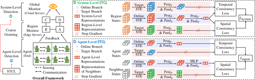
Figure 2: Overview of HiSTCLED. HiSTCLED contains three hierarchies, agents, region monitors, and a global monitor, which can be conceptually implemented by the end-edge-cloud collaborative framework. Agents sense the states of neighbors, measure the change in relationships, and communicate with them to make agent-level detection. The detecting results are coarse-grained to region states, whose spatial patterns are used for system-level detection. Representations of agents and the system are learned via spatio-temporal consistency learning (STCL) technique to support agent-level and system-level detection, respectively.

III-A Problem Formulation

Regarding the time steps when the emergence forms or evaporates as change points, emergence detection in CAS can be formulated as CPD in dynamic graphs as follows.

Definition 1 (Dyanmic graph).

A dynamic graph is composed of a graph series $\{\mathcal{G}^{t}\}^{T}_{t=1}$, where $\mathcal{G}^{t}=(\mathcal{V},\mathcal{E}^{t},\mathbf{X}^{t})$ is a snapshot at time $t$, with $\mathcal{V}$ as the set of nodes over all time steps, $\mathcal{E}^{t}$ as the set of edges at time $t$, and $\mathbf{X}^{t}$ as the node features at time $t$.

Definition 2 (CPD in dynamic graphs).

The task of CPD in dynamic graphs aims to find a set of change points $\mathcal{T}^{*}=\{t^{*}_{k}\}^{K}_{k=1}$ from a graph series $\{\mathcal{G}^{t}\}^{T}_{t=1}$. The change points split $[1,T]$ into contiguous segments such that $[1,T]=\bigcup^{K^{*}-1}_{k=1}[t^{*}_{k},t^{*}_{k+1}]$, with $t^{*}_{1}=1$ and $t^{*}_{K}=T$.

The node set $\mathcal{V}$ is assumed time-invariant for simplicity. One can always include nodes appearing at all time steps to form $\mathcal{V}$. The node feature $\mathbf{x}^{t}\in\mathbb{R}^{4}$ is an agent’s 2D position and velocity in this paper.

Under the distributed setting, the global monitor does not have direct access to agents’ states. Each agent as a local detector has limited vision and shares limited messages.

Definition 3 (Distributed Setting for Emergence Detection).

A qualified emergence detection method under the distributed setting should satisfy the following three conditions:

• Condition 1. An agent only senses the states of other agents within a certain radius. Formally, the neighborhood of agent $j$ at time $t$ is defined as $\mathcal{N}^{t}_{j}=\{i:d^{t}_{ij}\leq\delta\}$, where $d^{t}_{ij}$ is the Euclidean distance.

• Condition 2. An agent $j$ only communicates with its neighbors in $\mathcal{N}^{t}_{j}$.

• Condition 3. The only message that an agent $j$ shares with its neighbors or uploads to some monitor is its detecting score for emergence, i.e., a scalar $s^{t}_{j}\in[0,1]$.

Inspired by Ranshous et al. [34], this paper uses a dissimilarity function to calculate the detecting scores, and defines the criterion for CPD as follows.

Definition 4 (Criterion for CPD).

Given a graph series and a dissimilarity function $d(\mathcal{G},\mathcal{G}^{\prime})\in\mathbb{R}_{\geq 0}$, a change point $t$ is detected when $d(\mathcal{G}^{t},\mathcal{G}^{t-1})>c$ and $d(\mathcal{G}^{t},\mathcal{G}^{t+1})\leq c$ for some threshold $c$.

III-B Motivation and Overview of HiSTCLED

The distributed setting stated in Definition 3 poses severe challenges to existing spatio-temporal modeling techniques and emergence detection methods:

• Conditions 1 and 3 state that the hidden vectors of agents are not shared. Thus, the common practice of stacking multiple GNN layers [35] to capture long-range dependence over multi-hop neighbors is inapplicable.

• Conditions 2 and 3 state that it is hard to reach consensus among agents via local communication within a limited time, because the communication graph changes constantly and it is not necessarily connected [36]. See Appendix A for further demonstration.

• Condition 3 states that the global monitor is unable to make global detection by utilizing agents’ states in an end-to-end manner.

These challenges motivate the key design choice of HiSTCLED, that is, modeling the spatio-temporal dependency at different levels and aggregating the information hierarchically. An overview of HiSTCLED is shown in the left part of Figure 2. It contains three hierarchies from bottom-up, agents, region monitors, and a global monitor. It can be conceptually implemented by the end-edge-cloud collaborative framework [37]. The area where all agents move is split into several connected regions. In each region, every agent senses the states of its neighbors and detects if its relationship with neighbors changes significantly. Each agent communicates with its neighbors to enhance the agent-level detecting results. The detecting results of agents within the same region are aggregated by the corresponding region monitor. The regional results are analyzed by the global monitor to make a system-level detection that is aware of emergence-related patterns.

The agent-level and system-level detection are supported by agent-level and system-level representation learning, respectively. STEs are designed to capture nonlinear agent-to-agent and region-to-region relationships. Self-supervised learning strategies are designed to learn agent representations and the system representation that preserve spatio-temporal consistency. The inconsistency in system representation serves as a detection signal for emergence. Formally, HiSTCLED can be described as a three-step process, corresponding to its three-level structure,

$$\mathbf{s}^{1:T} =\text{AgentDetect}\left(\mathbf{X}^{1:T}\right)\in\mathbb{R}^{T\times|\mathcal{V}|},$$ (1)

$$\mathbf{y}^{1:T} =\text{CoarseGrain}\left(\mathbf{s}^{1:T}\right)\in\mathbb{R}^{T\times M},$$

$$s^{1:T}_{\mathcal{G}} =\text{SystemDetect}\left(\mathbf{y}^{1:T}\right)\in\mathbb{R}^{T}.$$

$\mathbf{s}^{1:T}$ are agent-level detecting scores, which are coarse-grained to $M$ regions’ states $\mathbf{y}^{1:T}$. $s^{1:T}_{\mathcal{G}}$ are system-level detecting scores based on region states. The following sections will describe the process of HiSTCLED in detail.

III-C Agent-Level Detection

The procedure of agent-level detection is shown in the right bottom part of Figure 2.

III-C1 Spatio-Temporal Encoder

To make online detection at time $\tau$, each agent records its state and its neighbors’ states in the last $w$ time steps. Denoting $\tau(w)=\tau-w+1$ as the initial step of the time window, these states are transformed to agent representations by the agent-level STE,

$$\mathbf{h}^{\tau(w):\tau}_{j}=\text{STE}_{A}\left(\mathbf{x}^{\tau(w):\tau}_{j},\left\{\mathbf{x}^{t}_{i}:i\in\mathcal{N}^{t}_{j}\right\}^{\tau}_{t=\tau(w)}\right)\in\mathbb{R}^{w\times D},$$ (2)

Due to Conditions 1 and 3 of the distributed setting, each agent cannot acquire their neighbors’ latent representations. Thus, the popular design choice of integrated dynamic GNNs that model spatio-temporal entangled relations [38, 39] is inapplicable. Instead, this paper adopts a stacked architecture composed of a spatial transformer and a temporal transformer [40], disentangling spatial and temporal dependency.

The spatial transformer models the relationship between an agent and its neighbors at each time step. The state of an agent $\mathbf{x}^{t}_{j}$ is first embedded as a hidden vector through a single-layer perceptron, i.e., $\mathbf{e}^{t}_{j}=\text{Emb}(\mathbf{x}^{t}_{j})$. Then, a scaled-dot product attention mechanism [40] with a skip connection is applied to calculate the spatial representation

$$\mathbf{z}^{t}_{j}=\mathbf{e}^{t}_{j}+\sum_{i\in\mathcal{N}^{t}_{j}}\alpha^{t}_{ij}f_{V}\left(\mathbf{e}^{t}_{i}-\mathbf{e}^{t}_{j}\right).$$ (3)

$\mathbf{e}^{t}_{i}-\mathbf{e}^{t}_{j}$ measures the spatial difference between agent $j$ and its neighbor $i$ in the latent space. It may capture nonlinear relations that are not fully reflected in quantities of the raw space, e.g., relative positions and velocities. $f_{V}$ is a value function implemented by a linear mapping. $\alpha^{t}_{ij}=\text{softmax}(\{a^{t}_{ij}:i\in\mathcal{N}^{t}_{j}\})$ is the normalized attention score, with $a^{t}_{ij}$ defined as

$$a^{t}_{ij}=\frac{1}{\sqrt{D}}f_{Q}\left(\mathbf{e}^{t}_{j}\right)^{T}f_{K}\left(\mathbf{e}^{t}_{i}\right),$$ (4)

where $f_{Q}$ and $f_{V}$ are linear layers accounting for the query function and the key function, respectively.

The spatial transformer does not require temporal embeddings of neighbors within a time window, which is desirable because the neighbors frequently change.

The temporal transformer is instantiated as a standard transformer [40], because it is powerful for sequential modeling, and it allows parallel execution, which is favorable for online detection. At its core is a temporal attention mechanism that maps spatial representations to temporal representations,

$$\mathbf{h}^{\tau(w):\tau}_{j}=\text{softmax}\left(\frac{1}{\sqrt{D}}\mathbf{q}^{\tau(w):\tau}_{j}\left(\mathbf{k}^{\tau(w):\tau}_{j}\right)^{T}\right)\mathbf{v}^{\tau(w):\tau}_{j},$$ (5)

where $\mathbf{q}^{\tau(w):\tau}_{j},\mathbf{k}^{\tau(w):\tau}_{j}$ and $\mathbf{v}^{\tau(w):\tau}_{j}$ are query, key and value vectors transformed from $\mathbf{z}^{\tau(w):\tau}$, respectively.

Disentangling the spatial and temporal information also makes the spato-temporal encoder friendly to streaming data because the agent representations can be updated incrementally. As the time step $\tau$ increases by 1, only the current spatial representation $\mathbf{z}^{\tau+1}_{j}$ needs to be computed, while $\mathbf{z}^{\tau(w)+1:\tau}_{j}$ can be reused. For the temporal transformer, intermediate results like the unnormalized attention scores and the query vectors that only involve $\mathbf{z}^{\tau(w)+1:\tau}_{j}$ can be stored. The normalized attention scores and the temporal representations can be computed by further incorporating $\mathbf{z}^{\tau+1}_{j}$. Details can be found in Appendix C.

III-C2 Spatio-Temporal Consistency Learning (STCL)

Since the labels of emergence are rarely known a priori, this paper proposes to train STE in a self-supervised manner by preserving the spatio-temporal consistency of the agent representations. STCL is inspired by an influential non-contrastive method called bootstrapping your own latent (BYOL) [41], which avoids explicit negative samples by aligning different views of the same sample encoded by asymmetric neural networks. BYOL is briefly introduced in Appendix A.

Unlike BYOL that uses a single objective, STCL disentangles the learning objectives of temporal consistency and spatial consistency since they characterize different aspects of the dynamic system. For each aspect, an online network and a target network with asymmetric network structures are designed to process different views of the same agent. These views are constructed by leveraging the intrinsic spatial and temporal relations within the data other than data augmentation that may damage the spatio-temporal semantics [31]. Given a view of some agent, the online network is trained to align the output of the target network for another view.

In the following subsections, a symbol with a tilde stands for an element from the target branch, e.g., a vector $\widetilde{\mathbf{h}}$ and a function $\widetilde{f}$. Symbols without a tilde come from the online branch. A vector with a superscript $t$ is called a transient representation at time $t$, e.g., $\mathbf{h}^{t}$. A vector with a superscript $(\tau)$ stands for a short-term representation within a time window $[\tau(w),\tau]$, e.g., $\mathbf{h}^{(\tau)}$.

Temporal Consistency Loss

When emphasizing the temporal consistency, the agent representation $\mathbf{h}^{t}_{j}$ is mapped to a temporal space via the temporal projection $\text{Proj}_{T}$. The resulting vectors $\mathbf{v}^{t}_{j}$ are reduced to a short-term representation via a temporal pooling function $\text{Pool}_{T}$, mean pooling here:

$$\mathbf{v}^{t}_{j}=\text{Proj}_{T}\left(\mathbf{h}^{t}_{j}\right),\quad\mathbf{v}_{j}^{(\tau)}=\text{Pool}_{T}\left(\mathbf{v}^{\tau(w):\tau}_{j}\right).$$ (6)

To ensure that the short-term representation is consistent with the transient representations, and thus capturing the tendency within the time window, this paper minimizes the dissimilarity between them. The dissimilarity is defined as the complement of the cosine similarity,

$$d\left(\mathbf{v}_{j}^{(\tau)},\widetilde{\mathbf{h}}^{t}_{j}\right)=\frac{1}{2}\left(1-\text{cos}\left(\mathbf{v}_{j}^{(\tau)},\widetilde{\mathbf{h}}^{t}_{j}\right)\right).$$ (7)

Then, the temporal consistency loss is defined as the average temporal dissimilarity of all agents within the time window,

$$\mathcal{L}_{T}=\frac{1}{w|\mathcal{V}|}\sum_{j\in\mathcal{V}}\sum^{\tau}_{t=\tau(w)}d\left(\mathbf{v}_{j}^{(\tau)},\widetilde{\mathbf{h}}^{t}_{j}\right).$$ (8)

Spatial Consistency Loss

When emphasizing the spatial consistency, $\mathbf{h}^{t}_{j}$ is mapped to a spatial space via the spatial projection $\text{Proj}_{S}$. To avoid disturbing the optimization of the temporal counterpart, this paper further transforms the resulting vectors with a multi-layer perceptron (MLP) to construct an asymmetric branch, i.e.,

$$\mathbf{n}^{t}_{j}=\text{Proj}_{S}\left(\mathbf{h}^{t}_{j}\right),\quad\mathbf{m}_{j}^{(\tau)}=\text{Pool}_{T}\left(\text{MLP}\left(\mathbf{n}^{\tau(w):\tau}_{j}\right)\right).$$ (9)

By minimizing the dissimilarity between the short-term representation of each agent and its neighbors, the model learns to preserve spatial consistency, i.e.,

$$\mathcal{L}_{S}=\frac{1}{\kappa|\mathcal{V}|}\sum_{j\in\mathcal{V}}\sum_{i\in\mathcal{N}_{j}}d\left(\mathbf{m}_{j}^{(\tau)},\widetilde{\mathbf{n}}_{i}^{(\tau)}\right),$$ (10)

where $\mathcal{N}_{j}$ contains $\kappa$ random neighbors from the temporal neighborhood $\cup^{\tau}_{t=\tau(w)}\mathcal{N}^{t}_{j}$. The sampling probability of a neighbor is proportional to its frequency.

As $\text{STE}_{A}$ is responsible for representation, while $\text{Proj}_{T}$ and $\text{Proj}_{S}$ are responsible for projections, they are simply implemented as MLPs. Mean pooling is adopted for $\text{Pool}_{T}$ and $\text{Pool}_{S}$ for simplicity, and more advanced spatial pooling [35, 42] and temporal pooling [43] methods are left for future work.

Optimization

Combining the temporal consistency loss and the spatial consistency loss, the overall loss for agent-level learning is

$$\mathcal{L}_{\text{Agent}}=\mathcal{L}_{T}+\mathcal{L}_{S}.$$ (11)

Directly minimizing the above loss will lead to collapsed representations [41]. To avoid this, the parameters $\Theta_{A}$ of the online branch are optimized by a gradient-based algorithm, e.g., Adam [44], while parameters $\widetilde{\Theta}_{A}$ of the target branch are updated by exponential moving average [41],

$$\Theta_{A}\leftarrow\text{Opt}\left(\mathcal{L}_{\text{Agent}},\Theta_{A}\right),\quad\widetilde{\Theta}_{A}\leftarrow\eta\widetilde{\Theta}_{A}+(1-\eta)\Theta_{A},$$ (12)

where $\eta\in[0,1]$ is a decay rate. The final $\Theta_{A}$ for emergence detection is obtained when the iterative process converges.

III-C3 Communication

Although each agent can make detection independently, sharing the detecting scores will make the detection more robust. In DETect [7], an agent only communicates with a randomly selected neighbor. Taking a step further, our method allows each agent to update its own score $s^{t}_{j}$ by combining the scores of all neighbors and the dissimilarity between representations of adjacent steps,

$$s^{\tau+1}_{j}=\alpha\cdot d\left(\mathbf{h}^{(\tau)}_{j},\mathbf{h}^{(\tau-1)}_{j}\right)+\frac{(1-\alpha)}{|\mathcal{N}_{j}^{\tau}|+1}\sum_{i\in\mathcal{N}^{\tau}_{j}\cup\{j\}}s^{\tau}_{i}.$$ (13)

where $\mathbf{h}^{(\tau)}_{j}=p_{T}\left(\mathbf{h}^{\tau(w):\tau}\right)$. $\alpha\in[0,1]$ is a mixing coefficient. When $\alpha=1$, the messages from neighbors are ignored, and when $\alpha=0$, the agent is overwhelmed by its neighbors’ detecting scores. The communication cost can be controlled by setting a budget for the number of neighbors.

III-D Coarse Graining and System-Level Detection

The procedure of system-level detection is shown in the right top part of Figure 2.

III-D1 Coarse Graining

The area where all agents move is split into several adjacent regions $\{\mathcal{R}_{m}\}^{M}_{m=1}$ in a grid shape. The detecting scores of agents within a region are aggregated as the region’s state,

$$y^{t}_{m}=\sum_{j\in\mathcal{R}_{m}}s^{t}_{j}.$$ (14)

These regions form a region graph $\mathcal{RG}^{t}=(\mathcal{RV},\mathcal{RE},\mathbf{y}^{t})$, with $\mathcal{RV}$ as the set of regions, $\mathcal{RE}$ as the set of edges between regions, and $\mathbf{y}^{t}$ as the region states at time $t$. The formulation can be naturally extended to regions with irregular boundaries and complex graph structures [45, 46]. This paper considers grid-shape region graphs for a proof of concept, while more complex scenarios are left for future work.

III-D2 Region Representation

As in agent-level detection, a region-level ST $\text{STE}_{R}$ with a similar network structure is applied to the region graph for obtaining the representation $\mathbf{r}^{t}_{m}$ for each region, i.e.,

$$\mathbf{r}^{\tau(w):\tau}_{m}=\text{STE}_{R}\left(y^{\tau(w):\tau}_{m},\left\{y^{t}_{n}:n\in\mathcal{RN}_{m}\right\}^{\tau}_{t=\tau(w)}\right),$$ (15)

where $\mathcal{RN}_{m}$ is the set of region $m$’s neighboring regions. Based on region representations, a system representation is learned to gain a global view of the system. Hence, the variation in system representations indicates the formation or evaporation of emergence. Likewise, temporal and spatial consistency losses are designed to guide the learning procedure.

III-D3 Spatio-Temporal Consistency Learning

Temporal Consistency Loss

A regional spatial projection $\text{Proj}_{RS}$ with a regional spatial pooling function $\text{Pool}_{RS}$ is applied to obtain the transient system representation,

$$\mathbf{r}^{t}_{\mathcal{G}}=\text{Pool}_{RS}\left(\left\{\text{Proj}_{RS}\left(\mathbf{r}^{t}_{m}\right):m\in\mathcal{RV}\right\}\right).$$ (16)

Then, a regional temporal projection $\text{Proj}_{RT}$ followed by a regional temporal pooling function $\text{Pool}_{RT}$ is applied to obtain the short-term system representation,

$$\mathbf{u}^{(\tau)}=\text{Pool}_{RT}\left(\text{Proj}_{RT}\left(\mathbf{r}^{\tau(w):\tau}_{\mathcal{G}}\right)\right).$$ (17)

By minimizing the dissimilarity between $\mathbf{u}^{(\tau)}$ and $\widetilde{\mathbf{r}}^{t}_{\mathcal{G}}$, the model learns to preserve system-level temporal consistency,

$$\mathcal{L}_{ST}=\frac{1}{w}\sum^{\tau}_{t=\tau(w)}d\left(\mathbf{u}^{(\tau)},\widetilde{\mathbf{r}}^{t}_{\mathcal{G}}\right).$$ (18)

Spatial Consistency Loss

The system-level spatial consistency loss ensures that the system representation $\mathbf{u}^{(\tau)}$ is consistent with the representation of each region. A regional spatial projection $\text{Proj}_{RS}$ together with a regional temporal pooling function $\text{Pool}_{RT}$ is applied to obtain the region representation within a time window,

$$\widetilde{\mathbf{w}}_{m}^{(\tau)}=\text{Pool}_{RT}\left(\widetilde{\text{Proj}}_{RS}\left(\widetilde{\mathbf{r}}^{\tau(w):\tau}_{m}\right)\right).$$ (19)

By minimizing the dissimilarity between $\mathbf{u}^{(\tau)}$ and $\widetilde{\mathbf{w}}_{m}^{(\tau)}$, the characteristics of each region are preserved in the system representation,

$$\mathcal{L}_{SS}=\frac{1}{\kappa}\sum_{m\in\mathcal{D}}d\left(\mathbf{u}^{(\tau)},\widetilde{\mathbf{w}}_{m}^{(\tau)}\right),$$ (20)

where $\mathcal{D}$ contains $\kappa$ sampled regions from $\mathcal{RV}$. For simplicity, $\text{Proj}_{ST}$ and $\text{Proj}_{SS}$ are implemented as MLPs, while $\text{Pool}_{RT}$ and $\text{Pool}_{RS}$ are mean pooling, as in agent-level detection.

The overall loss for system-level learning is the sum of temporal consistency loss and spatial consistency loss

$$\mathcal{L}_{\text{System}}=\mathcal{L}_{ST}+\mathcal{L}_{SS}.$$ (21)

The parameters of region-level online and target networks are updated in the same way as Eq. (12). Currently, agent-level and system-level STCL are trained separately. The reasons are twofold: (1) the construction of region states requires high-quality agent-level detecting scores; (2) it is hard to define meaningful system-level training signal for agent-level models without the truth change points. A joint optimization of the two hierarchies is left for future work.

The system-level detecting score is defined as the dissimilarity between system representations of adjacent time steps,

$$s^{\tau}_{\mathcal{G}}=d\left(\mathbf{u}^{(\tau)},\mathbf{u}^{(\tau-1)}\right).$$ (22)

A summary of notations used in this paper is shown in Appendix B. The pseudo codes for STCL and emergence detection are shown in Appendix C.

III-E Time Complexity Analysis of HiSTCLED

At the agent level, the time complexity of spatial encoding at time $t$ is $O(|\mathcal{E}^{t}|)$, and the time complexity of temporal encoding within a time window is $O(|\mathcal{V}|w^{2})$. Thus, the total complexity of spatio-temporal encoding is $O(|\mathcal{V}|w^{2}+\sum^{\tau}_{t=\tau(w)}|\mathcal{E}^{t}|)$. The time complexity for evaluating the temporal consistency loss and the spatial consistency loss is $O(w|\mathcal{V}|)$ and $O(\kappa|\mathcal{V}|)$. The time complexity of communication is $O(|\mathcal{E}^{t}|)$ at each time step. Therefore, at both the training and inference stages, the time complexity is linear of the number of agents and the number of edges.

Similarly, the time complexity of system-level spatio-temporal encoding is $O(|\mathcal{RV}|w^{2}+|\mathcal{RE}|w)$. The complexity of evaluating system-level temporal consistency loss and spatial consistency loss are $O(w)$ and $O(\kappa)$, respectively.

III-F Characteristics of HiSTCLED

HiSTCLED is characterized by the following features.

• By hierarchically aggregating agent-level detecting results, HiSTCLED can capture emergence-related spatial patterns ignored by DETect, where agents’ feedback is summed up indiscriminately.

• Thanks to the spatio-temporal disentangled architecture, STE can capture agents’ nonlinear relationships under the distributed setting, where popular designs of spatio-temporal integrated GNNs are infeasible.

• STCL preserves the spatio-temporal consistency within both agent-level and system-level representations. Compared with BYOL, it avoids potentially harmful data augmentations, and can handle multiple objectives in a disentangled way. It is free of negative samples, significantly reducing the computational cost for spatio-temporal data.

IV Experiments

IV-A Datasets

Evaluating the performance of online emergence detection methods generally requires building simulation environments to simulate the state evolution of agents. This paper adopts three simulation environments from DETect [7] implemented by NetLogo [47]. They are equipped with well-known yet hard-to-detect emergent phenomena. Agents move in a 2D bounded world composed of patches. The resulting datasets are briefly described as follows.

• Flock [48]: Each agent is a bird. The emergence is the flocking behavior. The objective measure of emergence is the number of patches that contain no birds.

• Pedestrian [11]: Each agent is a pedestrian walking either from left to right or in the opposite position. The emergence is the counter-flow. The objective measure of emergence is the number of lanes formed by pedestrians.

• Traffic [7]: Each agent is a car running on the road net of Manhattan, New York City. The road net contains 6,657 junctions and 77,569 road segments. The cars are routed by a routing engine GraphHopper [49] based on real-world car records. The emergence happens when a significant number of streets get congested. Thus, the objective measure of emergence is the number of congested road segments.

On Flock and Pedestrian datasets, real-world data is unavailable. Thus, reasonable behavioral rules are designed for agents. On Traffic dataset, the real-world data is combined with simulation rules to mimic agents’ behaviors. Visualizations of emergent behaviors on all datasets are shown in Appendix D. A summary of important statistics of the datasets is shown in Table I. Each dataset contains 20 times of simulations, with 5 times as the training set, 5 times as the validation set, and the rest as the testing set. Following O’toole et al. [7], the objective measure is evaluated every 50 steps. The ground truth change points are labeled by running offline CPD algorithms provided by ruptures [50]. Offline CPD algorithms have access to the whole series, and thus the labeled change points are more reliable and accurate. The results are checked manually. It turns out that change points make up no more than 1% of all evaluation steps. The severe imbalance between change points and normal points increases the challenge of emergence detection.

TABLE I: Statistics of datasets.

Datasets	Flock	Pedestrian	Traffic
# Agents	150	382	2,522
Shape of grid	$51\times 51$	$40\times 40$	$841\times 841$
# Simulation steps	50,000	50,000	60,000
# Evaluation steps	1,000	1,000	1,200
# Change points	10	10	$\approx$ 10

IV-B Evaluation Metrics

Due to the unpredictability of emergence, it can be difficult to detect the exact change points. The formation or evaporation of emergence can happen in a short period rather than a specific time step. Therefore, it is reasonable to accept more than one detection around a true change point in practice. In this paper, the detections within a given tolerance $\theta$ are regarded as one true positive (TP), while the rest detections are regarded as negative positive (FP), i.e.,

TP $$=\left|\left\{t^{*}\in\mathcal{T}^{*}:\exists t\in\widehat{\mathcal{T}},\text{s.t.}\,|t-t^{*}|\leq\theta\right\}\right|,$$

FP $$=\left|\left\{t\in\widehat{\mathcal{T}}:\forall t^{*}\in\mathcal{T}^{*},|t-t^{*}|>\theta\right\}\right|,$$

where $\mathcal{T}^{*}$ and $\widehat{\mathcal{T}}$ are the set of true change points and the set of detected ones, respectively. This paper sets $\theta=20$ for all datasets. Defining the precision $\text{Prec}=\frac{\text{TP}}{\text{TP}+\text{FP}}$ and the recall rate $\text{Rec}=\frac{\text{TP}}{|\mathcal{T}^{*}|}$, the F1 score can be computed as

$$\text{F1}=\frac{2\times\text{Prec}\times\text{Rec}}{\text{Prec}+\text{Rec}}.$$

The F1 score measures the overall accuracy of CPD. This paper further uses the covering metric [51, 52] to measure the overlapping degree between the ground truth segments and the detected segments. Let $\mathcal{A}^{*}$ be the set of ground truth segments $\mathcal{I}^{*}$, with a similar definition for $\widehat{\mathcal{A}}$ and $\widehat{\mathcal{I}}$. The covering metric is defined as

$$\text{Cover}\left(\mathcal{A}^{*},\widehat{\mathcal{A}}\right)=\frac{1}{T}\sum_{\mathcal{I}^{*}\in\mathcal{A}^{*}}|\mathcal{I}^{*}|\cdot\underset{\widehat{\mathcal{I}}\in\widehat{\mathcal{A}}}{\text{max}}\,J\left(\mathcal{I}^{*},\widehat{\mathcal{I}}\right),$$

where $J\left(\mathcal{I}^{*},\widehat{\mathcal{I}}\right)=\frac{\left|\mathcal{I}^{*}\cap\widehat{\mathcal{I}}\right|}{\left|\mathcal{I}^{*}\cup\widehat{\mathcal{I}}\right|}$ is the Jaccard index [53] measuring the overlapping degree between two segments.

In the original paper of DETect [7], the detecting performance is quantitatively evaluated by checking if the number of detected events is significantly larger during the emergent periods than the non-emergent periods. Nonetheless, the deviation between detected change points and the ground truth is not assessed. Therefore, this paper hopes to fill the gap by introducing the two metrics, and push the current research towards more timely emergence detection.

IV-C Baselines

To demonstrate the effectiveness of our method, this paper compares it with DETect and some state-of-the-art deep learning methods in closely related fields, including time series CPD method TS-CPP [54], time series AD method GDN [24], and graph-level AD method OCGTL [27]. Advanced techniques like GNNs and contrastive learning are used in these methods. They are adapted to our framework at both agent-level and system-level detection. They are renamed with a suffix “+HED”, short for Hierarchical Emergence Detection.

• DETect: A decentralized method for online emergence detection. Each agent detects the change in relationships between its neighbors and itself via a linear model. The detecting results are aggregated to make a global decision.

• TS-CPP+HED: A time series CPD method based on contrastive learning. Temporal convolutional networks [55] are used for time series encoding, and the similarity between two contiguous time segments is used as the indicator for CPD.

• GDN+HED: A GNN-based method for multi-variate time series AD. It uses graph attention to capture the relationships between sensors and defines the maximum deviation score for AD.

• OCGTL+HED: A graph-level AD method that combines one-class classification and neural transformation learning [56], an advanced self-supervised learning technique.

The codes of all baselines are publicly available. The code of DETect is directly applied to our experiments. The code of TS-CPP, GDN and OCGTL are adapted to our framework. Implementation details of HiSTCLED are described in Appendix D.

IV-D Comparison with Baselines

TABLE II: Detecting performance of different methods. Both the mean value and the standard deviation are reported. The best results are in bold. The improvements are significant ($p$-value $<0.05$). The relative improvements are computed w.r.t. DETect.

Datasets	Flock		Pedestrian		Traffic
Metrics	F1$\uparrow$	Cover$\uparrow$	F1$\uparrow$	Cover$\uparrow$	F1$\uparrow$	Cover$\uparrow$
TS-CPP+HED	0.7003$\pm$ 0.0029	0.6444$\pm$ 0.0148	0.7105$\pm$ 0.0260	0.6720$\pm$ 0.0320	0.3673$\pm$ 0.0370	0.5315$\pm$ 0.0313
GDN+HED	0.6755$\pm$ 0.0441	0.6902$\pm$ 0.0254	0.7181$\pm$ 0.0319	0.7123$\pm$ 0.0132	0.3473$\pm$ 0.0067	0.5276$\pm$ 0.0040
OCGTL+HED	0.7092$\pm$ 0.0301	0.7299$\pm$ 0.0437	0.9248$\pm$ 0.0207	0.8854$\pm$ 0.0134	0.3674$\pm$ 0.0379	0.5713$\pm$ 0.0194
DETect	0.4862$\pm$ 0.0507	0.6559$\pm$ 0.0284	0.2064$\pm$ 0.0807	0.4408$\pm$ 0.0416	0.3479$\pm$ 0.0875	0.5479$\pm$ 0.0558
HiSTCLED	0.7757$\pm$ 0.0026	0.7810$\pm$ 0.0116	0.9352$\pm$ 0.0096	0.9235$\pm$ 0.0107	0.3928$\pm$ 0.0235	0.5872$\pm$ 0.0093
Improvement	+59.54%	+19.07%	+353.10%	+109.51%	+12.91%	+7.17%

The detecting performance of different methods are shown in Table II. The metrics of DETect are relatively low on all datasets, showing that emergence detection can be difficult for traditional methods even on the simulation datasets. Deep learning methods generally outperform DETect in both metrics, and HiSTCLED achieves the highest performance. The results verify the superiority of our framework, which can capture emergence-related spatial patterns and model nonlinear spatio-temporal dynamics. GDN+HED calculates the detecting score based on next-step prediction error, which can be sensitive to the noise in the states. HiSTCLED calculates the score based on the consistency of representations, which is resistant to potential noise. HiSTCLED jointly preserves spatial and temporal consistency, and thus outperforms TS-CPP+HED that ignores spatial consistency and OCGTL+HED that ignores temporal consistency.

IV-E Ablation Study

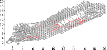
(a) States of road nets.

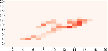
(b) States of regions.

Figure 3: Case study of spatial patterns on Traffic dataset. In (a), each line segment represents a road segment. Segments in red are congested, while those in gray are normal. In (b), each grid represents a region state. The darker the color, the more agent-level detections are collected. Best viewed in color.

Some variants of HiSTCLED are introduced to verify the necessity of capturing emergence-related patterns and modeling agents’ relationships with neighbors. HiSTCLED${}_{\text{Agent}}$ removes system-level detection. HiSTCLED${}_{\text{Self}}$ makes agent-level detection without modeling the spatial relationships, i.e., removing the spatial encoder and training without the spatial consistency loss. The Results are shown in Table III.

Effect of System-Level Detection

Without system-level detection, the average F1 score and the covering metric of HiSTCLED${}_{\text{Agent}}$ decrease by 0.0943 and 0.0970, respectively. The results verify that the spatial patterns of agent-level detecting results help with emergence detection.

To see what patterns are captured by HiSTCLED, a case study is conducted on Traffic dataset. Figure 3 visualizes the congesting states of the road net and the region states when the network-level congestion forms. Figure 3(a) shows that congested road segments constitute a connected subnetwork with a diameter of 80, accounting for more than $\frac{1}{3}$ of the diameter of the road net. The phenomenon confirms the emergence of widespread congestion. Such emergence-related pattern is almost faithfully reflected in region states. The results also show that HiSTCLED can detect the emergence of widespread congestion even when the traffic flow is not provided.

Effect of Agent-Level Detection

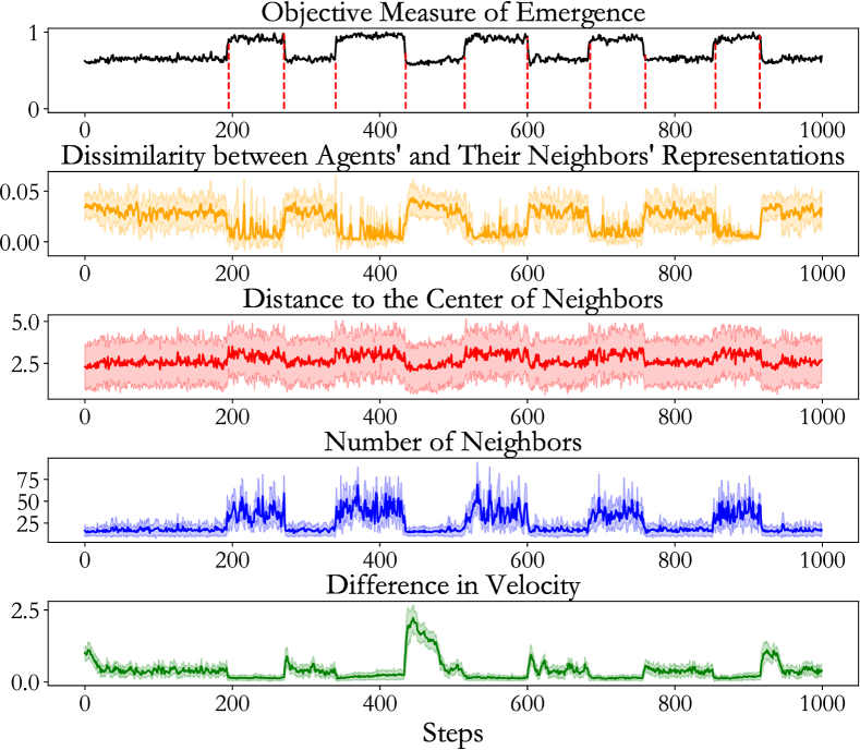
Figure 4: Case study of agents’ relationships on Flock dataset. The variation curves of the objective measure, agents’ dissimilarity in latent space, and agents’ relationships w.r.t. three indicators are visualized. Best viewed in color.

Compared with HiSTCLED${}_{\text{Agent}}$, the average F1 score and the covering metric of HiSTCLED${}_{\text{Self}}$ decrease by 0.0264 and 0.0171, respectively. The results show that modeling the nonlinear relationship between an agent and its neighbors is indispensable for agent-level detection. Note that HiSTCLED${}_{\text{Agent}}$ is better than DETect on Flock and Pedestrian datasets, and on par with it on Traffic dataset, which again verifies the effectiveness of agent-level spatio-temporal modeling.

To see how HiSTCLED${}_{\text{Agent}}$ captures the relationships, this paper conducts a case study on Flock dataset. Inspired by O’toole et al. [7], three indicators are used to measure the relationships w.r.t. agents’ states, including the distance to the center of neighbors, the number of neighbors, and the difference between an agent’s velocity and its neighbors’ average velocity. The objective measure of emergence is set as a reference. Agents’ and their neighbors’ dissimilarity in representations stands for relationships in the latent space. The variation curves of the aforementioned metrics are shown in Figure 4. As expected, during the emergent period of flocking, birds get crowded, and thus, the distances are smaller, the neighbor count increases, and the difference in velocity decreases. Different metrics present different patterns, yet these patterns are approximately captured by the latent representations. The tendency of the dissimilarity curve also agrees with that of the objective measure. These results show that our method can somehow capture the relationships defined by some intuitive metrics w.r.t. agents’ states.

TABLE III: Abalation study. Both the mean value and the standard deviation are reported. The best results of agent-level and system-level detection are in bold. The improvements are significant ($p$-value $<0.05$).

Datasets	Flock		Pedestrian		Traffic
Metrics	F1$\uparrow$	Cover$\uparrow$	F1$\uparrow$	Cover$\uparrow$	F1$\uparrow$	Cover$\uparrow$
HiSTCLED${}_{\text{Agent-S}}$	0.6351$\pm$ 0.0451	0.6962$\pm$ 0.0438	0.7627$\pm$ 0.0556	0.7430$\pm$ 0.0361	0.3189$\pm$ 0.0265	0.5319$\pm$ 0.0106
HiSTCLED${}_{\text{Agent-T}}$	0.6264$\pm$ 0.0271	0.6847$\pm$ 0.0275	0.7773$\pm$ 0.0119	0.7490$\pm$ 0.0250	0.3197$\pm$ 0.0361	0.5227$\pm$ 0.0164
HiSTCLED${}_{\text{Agent}}$	0.6705$\pm$ 0.0114	0.6960$\pm$ 0.0168	0.7965$\pm$ 0.0163	0.7601$\pm$ 0.0108	0.3538$\pm$ 0.0027	0.5445$\pm$ 0.0090
HiSTCLED${}_{\text{S}}$	0.7155$\pm$ 0.0317	0.7516$\pm$ 0.0169	0.9220$\pm$ 0.0142	0.9089$\pm$ 0.0199	0.3690$\pm$ 0.0266	0.5755$\pm$ 0.0361
HiSTCLED${}_{\text{T}}$	0.7564$\pm$ 0.0620	0.7680$\pm$ 0.0310	0.9278$\pm$ 0.0122	0.9082$\pm$ 0.0187	0.3735$\pm$ 0.0233	0.5880$\pm$ 0.0219
HiSTCLED${}_{\text{Self}}$	0.6413$\pm$ 0.0303	0.6899$\pm$ 0.0319	0.7732$\pm$ 0.0128	0.7211$\pm$ 0.0325	0.3271$\pm$ 0.0227	0.5382$\pm$ 0.0088
HiSTCLED	0.7757$\pm$ 0.0026	0.7810$\pm$ 0.0116	0.9352$\pm$ 0.0096	0.9235$\pm$ 0.0107	0.3928$\pm$ 0.0235	0.5872$\pm$ 0.0093

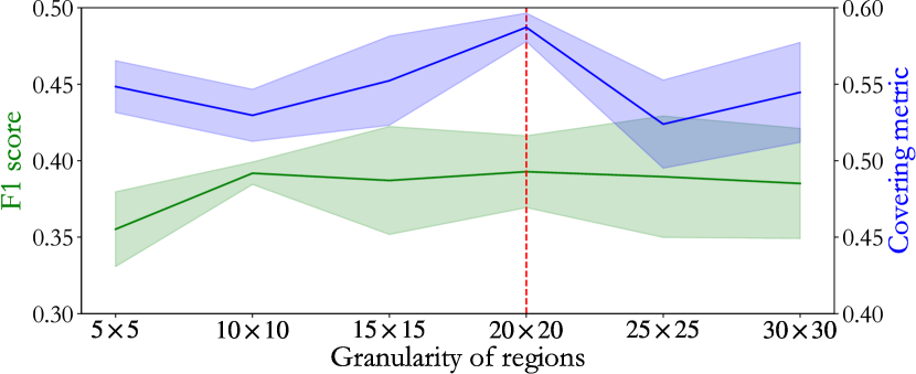
Figure 5: Effect of region granularity on Traffic dataset. The dashed vertical line indicates the best results. Best viewed in color.

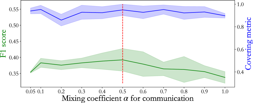
Figure 6: Effect of agents’ communication on Traffic dataset. The dashed vertical line indicates the best results. Best viewed in color.

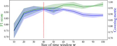
Figure 7: Effect of window size in system-level detection on Pedestrian dataset. Best viewed in color.

Effect of Spatial and Temporal Consistency Losses

To validate the effectiveness of STCL for both agent-level and system-level detection, this paper introduces variants of HiSTCLED${}_{\text{Agent}}$ and HiSTCLED trained with only the spatial or the temporal consistency loss. The resulting methods are denoted as HiSTCLED${}_{\text{Agent-S}}$, HiSTCLED${}_{\text{Agent-T}}$, HiSTCLED${}_{\text{S}}$, and HiSTCLED${}_{\text{T}}$, respectively. As shown in Table III, removing any term in the loss function will lead to degenerated performance in most cases. Thus, the spatial consistency loss and temporal consistency loss are complementary to learning discriminative representations for emergence detection.

IV-F Hyperparameter Analysis

Effect of Region Granularity

The area where agents move is split into many regions for system-level detection. The granularity of regions decides how many details are preserved for global analysis. To study the effect of region granularity, this paper trains the system-level detector on Traffic dataset under several $N\times N$ grids, with $N\in\{5,10,15,20,25,30\}$. The results are shown in Figure 6. The F1 score is lowest when $N=5$. Maybe coarsening too much will result in inadequate information that cannot support accurate detection. Both the F1 score and covering metric increase as $N$ grows but start to decrease at $N=20$. When $N$ is too large, the regions are too small to collect sufficient feedback from agents and present stable spatial patterns. Thus, our method achieves the highest performance for $N=20$ with a moderate computational cost.

Effect of Mixing Coefficient for Communication

Agents communicate with neighbors to make agent-level detections. The mixing coefficient $\alpha$ in Eq. (13) balances the importance of an agent’s current observation and its neighbors’ detecting scores. $\alpha$ is set to $0.05$ to keep consistent with DETect. To see how $\alpha$ affects the detecting accuracy, this paper evaluates HiSTCLED${}_{\text{Agent}}$ on Traffic dataset with $\alpha$ ranging from $0.1$ to $1$. As shown in Figure 6, the F1 score and covering metric can be promoted by increasing $\alpha$, i.e., assigning a larger weight to agents’ current observation. However, when $\alpha=1$, i.e., agents ignore the detecting scores of their neighbors, the F1 score drops significantly, verifying the necessity of communication. The results show the possibility of tuning $\alpha$ to improve the detecting accuracy. Furthermore, $\alpha$ can be personalized and adaptive over time. Optimizing the choices of $\alpha$ is left for future work.

Effect of Window Size for Emergence Detection

The window size $w$ is the temporal scope of emergence detection. Like the granularity of regions, there is a tradeoff between precision and efficacy w.r.t. $w$. It is set to $10$ for agent-level detection, since the objective measure of emergence is evaluated every 50 steps and the states of agents are downsampled every 5 steps. In this way, agents can make relatively accurate and timely detections. However, performance degeneration is observed for system-level detection with the same window size. It is conjectured that system-level needs a larger temporal scope with coarse-grained spatial information. The effect of $w$ is studied on Pedestrian dataset, with $w\in\{10,20,\dots,100\}$. As shown in Figure 7, the F1 score generally increases as $w$ grows, while the covering metric peaks at $w=40$. Therefore, to achieve better overall performance with a moderate computational cost, $w$ is set to 40 for system-level detection. This choice is also practical since the global monitor generally has a larger capacity than a single agent.

Effect of Threshold $\theta$

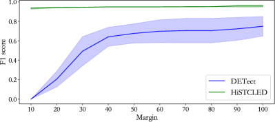
Figure 8: Effect of threshold $\theta$ on Pedestrian dataset. Best viewed in color.

In the experiments, the threshold $\theta$ is set to $20$ on all datasets for fairly comparing the detecting precision of different methods. Apparently, the F1 scores are affected by the choices of $\theta$. This paper evaluate the F1 scores of HiSTCLED and DETect on Pedestrian dataset for $\theta\in\left\{10,20,\dots,100\right\}$, and the results are shown in Figure 8. For both methods, the F1 score grows approximately as $\theta$ increases, because a larger tolerance allows to include more detected change points. On the whole, HiSTCLED consistently achieves higher detecting precision than DETect for all $\theta$, yet the difference narrows down as $\theta$ increases. Besides, the variance of DETect’s F1 scores tends to grow up for a larger $\theta$, while HiSTCLED preserves a considerably smaller variance, showing that the performance of HiSTCLED is more stable. In practice, a relatively smaller threshold is more favorable, because detected change points with smaller displacement help to detect the emergence more timely.

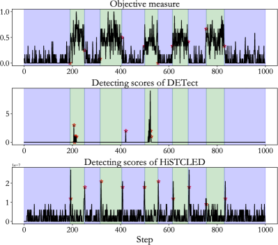
Figure 9: Visualization of the ground truth change points (top), and change points detected by DETect (middle) and HiSTCLED (bottom) on Pedestrian dataset. The variation curves are in black. The change points are marked as stars. The periods of emergence are in green. The normal periods are in purple. Best viewed in color.

To further differentiate the detecting quality of DETect and HiSTCLED, this paper visualizes their detected change points on Pedestrian dataset. As shown in Figure 9, DETect fails to detect change points in several periods, and the detected points are relatively far from the nearest ground truth. By contrast, HiSTCLED successfully detects all change points with significantly smaller deviations.

V Conclusion

This paper proposes a hierarchical framework named HiSTCLED for emergence detection in CAS under the distributed setting. By aggregating agent-level detecting results from bottom-up, HiSTCLED learns a system representation that captures emergence-related patterns. Nonlinear relationships between agents and their neighbors are encoded in agent representations through STE. These representations are learned in a self-supervised manner by preserving the spatio-temporal consistency. HiSTCLED surpasses the traditional methods and deep learning methods on three datasets with well-known yet hard-to-detect emergent phenomena. HiSTCLED is flexible to incorporate deep learning methods from graph-level CPD and anomaly detection for effective emergence detection.

Future work includes introducing distributed GNNs and advanced CPD methods to boost the performance of emergence detection. Designing graph learning methods for emergence-related higher-order structures is also promising. Besides, it is crucial to construct more realistic simulation environments to evaluate the performance and identify real-world challenges.

References

- Artime and De Domenico [2022] O. Artime and M. De Domenico, “From the origin of life to pandemics: Emergent phenomena in complex systems,” Philosophical Transactions of the Royal Society A, vol. 380, no. 2227, p. 20200410, 2022.
- Kalantari et al. [2020] S. Kalantari, E. Nazemi, and B. Masoumi, “Emergence phenomena in self-organizing systems: A systematic literature review of concepts, researches, and future prospects,” Journal of Organizational Computing and Electronic Commerce, vol. 30, no. 3, pp. 224–265, 2020.
- O’toole [2016] E. O’toole, “Decentralised detection of emergence in complex adaptive systems,” Ph.D. dissertation, Trinity College (Dublin, Ireland), 2016.
- Fromm [2005] J. Fromm, “Types and forms of emergence,” arXiv preprint nlin/0506028, 2005.
- Bedau [1997] M. A. Bedau, “Weak emergence,” Philosophical Perspectives, vol. 11, pp. 375–399, 1997.
- Zeng et al. [2021] G. Zeng, Z. Sun, S. Liu, X. Chen, D. Li, J. Wu, and Z. Gao, “Percolation-based health management of complex traffic systems,” Frontiers of Engineering Management, vol. 8, no. 4, pp. 557–571, 2021.
- O’toole et al. [2017] E. O’toole, V. Nallur, and S. Clarke, “Decentralised detection of emergence in complex adaptive systems,” ACM Transactions on Autonomous and Adaptive Systems, vol. 12, no. 1, pp. 1–31, 2017.
- Aminikhanghahi and Cook [2016] S. Aminikhanghahi and D. J. Cook, “A survey of methods for time series change point detection,” Knowledge and Information Systems, vol. 51, pp. 339–367, 2016.
- Gignoux et al. [2017] J. Gignoux, G. Chérel, I. D. Davies, S. R. Flint, and E. Lateltin, “Emergence and complex systems: The contribution of dynamic graph theory,” Ecological Complexity, vol. 31, pp. 34–49, 2017.
- Mnif and Müller-Schloer [2011] M. Mnif and C. Müller-Schloer, “Quantitative emergence,” in Organic Computing—A Paradigm Shift for Complex Systems. Springer, 2011, pp. 39–52.
- Procházka and Olševičová [2015] J. Procházka and K. Olševičová, “Monitoring lane formation of pedestrians: Emergence and entropy,” in Asian Conference on Intelligent Information and Database Systems. Springer, 2015, pp. 221–228.
- Liu et al. [2018] Q. Liu, M. He, D. Xu, N. Ding, and Y. Wang, “A mechanism for recognizing and suppressing the emergent behavior of UAV swarm,” Mathematical Problems in Engineering, vol. 2018, 2018.
- Luo et al. [2022] J. Luo, J. Xin, G. Binghui, H. Zheng, W. Wu, and W. Lv, “Dynamic model and crowd entropy measurement of crowd intelligence system (in Chinese with English abstract),” SCIENTIA SINICA Informationis, vol. 52, no. 1, pp. 99–110, 2022.
- Fisch et al. [2010] D. Fisch, M. Jänicke, B. Sick, and C. Müller-Schloer, “Quantitative emergence–A refined approach based on divergence measures,” in Fourth IEEE International Conference on Self-Adaptive and Self-Organizing Systems. IEEE Computer Society, 2010, pp. 94–103.
- Seth [2008] A. K. Seth, “Measuring emergence via nonlinear granger causality.” in ALIFE, vol. 2008, 2008, pp. 545–552.
- Grossman et al. [2008] R. L. Grossman, M. Sabala, Y. Gu, A. Anand, M. Handley, R. Sulo, and L. Wilkinson, “Discovering emergent behavior from network packet data: Lessons from the angle project,” in Next Generation of Data Mining. Chapman and Hall/CRC, 2008, pp. 267–284.
- Niazi and Hussain [2011] M. A. Niazi and A. Hussain, “Sensing emergence in complex systems,” IEEE Sensors Journal, vol. 11, no. 10, pp. 2479–2480, 2011.
- Santos et al. [2017] E. Santos, Y. Zhao, and S. Gómez, “Automatic emergence detection in complex systems,” Complex., vol. 2017, 2017.
- Wang et al. [2017] Y. Wang, A. Chakrabarti, D. Sivakoff, and S. Parthasarathy, “Fast change point detection on dynamic social networks,” in Proceedings of the 26th International Joint Conference on Artificial Intelligence, 2017, pp. 2992–2998.
- Huang et al. [2020] S. Huang, Y. Hitti, G. Rabusseau, and R. Rabbany, “Laplacian change point detection for dynamic graphs,” in Proceedings of the 26th ACM SIGKDD International Conference on Knowledge Discovery & Data Mining, 2020, pp. 349–358.
- Sulem et al. [2023] D. Sulem, H. Kenlay, M. Cucuringu, and X. Dong, “Graph similarity learning for change-point detection in dynamic networks,” Machine Learning, vol. 113, pp. 1–44, 2023.
- Ma et al. [2023] X. Ma, J. Wu, S. Xue, J. Yang, C. Zhou, Q. Z. Sheng, H. Xiong, and L. Akoglu, “A comprehensive survey on graph anomaly detection with deep learning,” IEEE Transactions on Knowledge and Data Engineering, vol. 35, no. 12, pp. 12 012–12 038, 2023.
- Pazho et al. [2022] A. D. Pazho, G. A. Noghre, A. A. Purkayastha, J. Vempati, O. Martin, and H. Tabkhi, “A comprehensive survey of graph-based deep learning approaches for anomaly detection in complex distributed systems,” arXiv preprint arXiv:2206.04149, 2022.
- Deng and Hooi [2021] A. Deng and B. Hooi, “Graph neural network-based anomaly detection in multivariate time series,” in Proceedings of the AAAI Conference on Artificial Intelligence, vol. 35, no. 5, 2021, pp. 4027–4035.
- Zheng et al. [2023] Y. Zheng, H. Y. Koh, M. Jin, L. Chi, K. T. Phan, S. Pan, Y.-P. P. Chen, and W. Xiang, “Correlation-aware spatial–temporal graph learning for multivariate time-series anomaly detection,” IEEE Transactions on Neural Networks and Learning Systems, November 2023, doi: 10.1109/TNNLS.2023.3325667.
- Zhao and Akoglu [2023] L. Zhao and L. Akoglu, “On using classification datasets to evaluate graph outlier detection: Peculiar observations and new insights,” vol. 11, no. 3, pp. 151–180, 2023.
- Qiu et al. [2022] C. Qiu, M. Kloft, S. Mandt, and M. Rudolph, “Raising the bar in graph-level anomaly detection,” in Proceedings of the Thirty-First International Joint Conference on Artificial Intelligence, 2022, pp. 2196–2203.
- Protogerou et al. [2021] A. Protogerou, S. Papadopoulos, A. Drosou, D. Tzovaras, and I. Refanidis, “A graph neural network method for distributed anomaly detection in IoT,” Evolving Systems, vol. 12, no. 1, pp. 19–36, 2021.
- Wu et al. [2023] L. Wu, H. Lin, C. Tan, Z. Gao, and S. Z. Li, “Self-supervised learning on graphs: Contrastive, generative, or predictive,” IEEE Transactions on Knowledge and Data Engineering, vol. 35, no. 4, pp. 4216–4235, 2023.
- Tian et al. [2021] S. Tian, R. Wu, L. Shi, L. Zhu, and T. Xiong, “Self-supervised representation learning on dynamic graphs,” in Proceedings of the 30th ACM International Conference on Information & Knowledge Management, 2021, pp. 1814–1823.
- Liu et al. [2022a] X. Liu, Y. Liang, C. Huang, Y. Zheng, B. Hooi, and R. Zimmermann, “When do contrastive learning signals help spatio-temporal graph forecasting?” in Proceedings of the 30th International Conference on Advances in Geographic Information Systems, 2022, pp. 1–12.
- Pei et al. [2023] L. Pei, Y. Cao, Y. Kang, Z. Xu, and Z. Zhao, “Self-supervised spatiotemporal clustering of vehicle emissions with graph convolutional network,” IEEE Transactions on Neural Networks and Learning Systems, July 2023, doi: 10.1109/TNNLS.2023.3293463.
- Zhang et al. [2023] Q. Zhang, C. Huang, L. Xia, Z. Wang, Z. Li, and S. Yiu, “Automated spatio-temporal graph contrastive learning,” in Proceedings of the ACM Web Conference, 2023, pp. 295–305.
- Ranshous et al. [2015] S. Ranshous, S. Shen, D. Koutra, S. Harenberg, C. Faloutsos, and N. F. Samatova, “Anomaly detection in dynamic networks: A survey,” WIREs Computational Statistics, vol. 7, no. 3, pp. 223–247, 2015.
- Wu et al. [2020] Z. Wu, S. Pan, F. Chen, G. Long, C. Zhang, and S. Y. Philip, “A comprehensive survey on graph neural networks,” IEEE Transactions on Neural Networks and Learning Systems, vol. 32, no. 1, pp. 4–24, 2020.
- Ren and Beard [2008] W. Ren and R. W. Beard, Distributed consensus in multi-vehicle cooperative control. Springer, 2008, vol. 27, no. 2.
- He et al. [2022] Q. He, Z. Dong, F. Chen, S. Deng, W. Liang, and Y. Yang, “Pyramid: Enabling hierarchical neural networks with edge computing,” in Proceedings of the ACM Web Conference, 2022, pp. 1860–1870.
- Skarding et al. [2021] J. Skarding, B. Gabrys, and K. Musial, “Foundations and modeling of dynamic networks using dynamic graph neural networks: A survey,” IEEE Access, vol. 9, pp. 79 143–79 168, 2021.
- Wang et al. [2022] S. Wang, J. Cao, and P. S. Yu, “Deep learning for spatio-temporal data mining: A survey,” IEEE Transactions on Knowledge and Data Engineering, vol. 34, no. 8, pp. 3681–3700, 2022.
- Vaswani et al. [2017] A. Vaswani, N. Shazeer, N. Parmar, J. Uszkoreit, L. Jones, A. N. Gomez, Ł. Kaiser, and I. Polosukhin, “Attention is all you need,” Advances in Neural Information Processing Systems, vol. 30, pp. 5998–6008, 2017.
- Grill et al. [2020] J.-B. Grill, F. Strub, F. Altché, C. Tallec, P. Richemond, E. Buchatskaya, C. Doersch, B. Avila Pires, Z. Guo, M. Gheshlaghi Azar et al., “Bootstrap your own latent: A new approach to self-supervised learning,” Advances in Neural Information Processing Systems, vol. 33, pp. 21 271–21 284, 2020.
- Liu et al. [2022b] C. Liu, Y. Zhan, J. Wu, C. Li, B. Du, W. Hu, T. Liu, and D. Tao, “Graph pooling for graph neural networks: Progress, challenges, and opportunities,” arXiv preprint arXiv:2204.07321, 2022.
- Lee et al. [2021] D. Lee, S. Lee, and H. Yu, “Learnable dynamic temporal pooling for time series classification,” in Proceedings of the AAAI Conference on Artificial Intelligence, vol. 35, no. 9, 2021, pp. 8288–8296.
- Kingma and Ba [2015] D. P. Kingma and J. Ba, “Adam: A method for stochastic optimization,” in International Conference on Learning Representations, 2015.
- Sun et al. [2020] J. Sun, J. Zhang, Q. Li, X. Yi, Y. Liang, and Y. Zheng, “Predicting citywide crowd flows in irregular regions using multi-view graph convolutional networks,” IEEE Transactions on Knowledge and Data Engineering, vol. 34, no. 5, pp. 2348–2359, 2020.
- Li et al. [2022] F. Li, J. Feng, H. Yan, D. Jin, and Y. Li, “Crowd flow prediction for irregular regions with semantic graph attention network,” ACM Transactions on Intelligent Systems and Technology, vol. 13, no. 5, pp. 1–14, 2022.
- Tisue and Wilensky [2004] S. Tisue and U. Wilensky, “Netlogo: A simple environment for modeling complexity,” in International Conference on Complex Systems, vol. 21. Boston, MA, 2004, pp. 16–21.
- Reynolds [1987] C. W. Reynolds, “Flocks, herds and schools: A distributed behavioral model,” in Proceedings of the 14th Annual Conference on Computer Graphics and Interactive Techniques, M. C. Stone, Ed. ACM, 1987, pp. 25–34.
- [49] P. Karich and S. Schöder, “Graphhopper.” [Online]. Available: https://graphhopper.com/
- Truong et al. [2020] C. Truong, L. Oudre, and N. Vayatis, “Selective review of offline change point detection methods,” Signal Processing, vol. 167, p. 107299, 2020.
- Van den Burg and Williams [2020] G. J. Van den Burg and C. K. Williams, “An evaluation of change point detection algorithms,” arXiv preprint arXiv:2003.06222, 2020.
- Arbelaez et al. [2010] P. Arbelaez, M. Maire, C. Fowlkes, and J. Malik, “Contour detection and hierarchical image segmentation,” IEEE Transactions on Pattern Analysis and Machine Intelligence, vol. 33, no. 5, pp. 898–916, 2010.
- Jaccard [1912] P. Jaccard, “The distribution of the flora in the alpine zone. 1,” New Phytologist, vol. 11, no. 2, pp. 37–50, 1912.
- Deldari et al. [2021] S. Deldari, D. V. Smith, H. Xue, and F. D. Salim, “Time series change point detection with self-supervised contrastive predictive coding,” in Proceedings of the Web Conference, 2021, pp. 3124–3135.
- Bai et al. [2018] S. Bai, J. Z. Kolter, and V. Koltun, “An empirical evaluation of generic convolutional and recurrent networks for sequence modeling,” arXiv preprint arXiv:1803.01271, 2018.
- Qiu et al. [2021] C. Qiu, T. Pfrommer, M. Kloft, S. Mandt, and M. Rudolph, “Neural transformation learning for deep anomaly detection beyond images,” in International Conference on Machine Learning. PMLR, 2021, pp. 8703–8714.