Correspondence Analysis for Symbolic Multi–Valued Variables

Abstract

This paper sets a proposal of a new method and two new algorithms for Correspondence Analysis when we have Symbolic Multi–Valued Variables (SymCA). In our method, there are two multi–valued variables $X$ and $Y$, that is to say, the modality that takes the variables for a given individual is a finite set formed by the possible modalities taken for the variables in a given individual, that which allows to apply the Correspondence Analysis to multiple selection questionnaires. Then, starting from all the possible classic contingency tables an interval contingency table can be built, which will be the point of departure of the proposed method.

Symbolic data analysis, contingency tables, interval contingency table, disjunctive complete table, symbolic multi–valued variables.

1 Relationship between two symbolic multi–valued variables

One of the objectives of the Correspondence Analysis is to explore the relationships between the modalities of two qualitative variables by two–dimensional representations. The objective of the Correspondence Factorial Analysis between two symbolic multi–valued variables (SymCA) is the same one, but also there is some kind of uncertainty in the input data that will be reflected in the two–dimensional representations, since each modality will be represented with a rectangle instead of a point, as usual. A symbolic variable $Y$ is called multi–valued one if its values $Y(k)$ are all finite subsets [Bock and Diday (2000)].

In the classic Correspondence Analysis a contingency table associated with two qualitative variables is build. For example, suppose there are two qualitative variables: $X=$eyes-color (with 3 modalities green, blue and brown) and $Y=$ hair-color (with 2 modalities blond and black). If each one of the 2 qualitative variables is observed in 5 individuals the following disjunctive complete tables could be obtained:

$$X=\left[\begin{array}[]{ccc}1&0&0\\ 0&0&1\\ 1&0&0\\ 0&0&1\\ 1&0&0\end{array}\right],\qquad Y=\left[\begin{array}[]{cc}0&1\\ 0&1\\ 0&1\\ 1&0\\ 1&0\end{array}\right].$$

In these matrices, if the $(i,j)-$entry is 1, it means that the individual $i$ take the modality $j$ and a 0 means that individual $i$ doesn’t take it. If the matrix multiplication $K=X^{t}Y$ is made, the crossed table or contingency table between the variables $X$ and $Y$ will be obtained, such as the following:

$$K=X^{t}Y=\left[\begin{array}[]{cc}1&2\\ 0&0\\ 1&1\end{array}\right].$$

In the $(i,j)-$entry of the matrix $K$ appears the quantity of individuals that assume simultaneously the modality $i$ of the variable $X$ and the modality $j$ of the variable $Y$. As it is well known, the Correspondence Analysis usually starts up with the contingency table among the variables $X$ and $Y$.

For the case of multi–valued variables there will be individuals whose information regards the assumed modality is a “diffuse variable”.

Example 1. Let $X$ be the qualitative variable “eyes-color” with 3 modalities: green, blue and brown; it could be that the eyes color of the first individual is green or blue (but not both), that is to say $X(1)=$green or $X(1)=$blue. Let $Y$ be the qualitative variable “hair-color” with 2 modalities blond and black, there could also be an individual whose hair color is not completely well defined, for instance for the third individual, it might also be $Y(3)=$blond or $Y(3)=$black but not both). In this way there are two possible disjunctive complete tables for the variable $X$ and two for $Y$, which are:

$$X_{1}=\left[\begin{array}[]{ccc}1&0&0\\ 0&0&1\\ 1&0&0\\ 0&0&1\\ 1&0&0\end{array}\right],\quad X_{2}=\left[\begin{array}[]{ccc}0&1&0\\ 0&0&1\\ 1&0&0\\ 0&0&1\\ 1&0&0\end{array}\right],\qquad Y_{1}=\left[\begin{array}[]{cc}0&1\\ 0&1\\ 1&0\\ 1&0\\ 1&0\end{array}\right],\quad Y_{2}=\left[\begin{array}[]{cc}0&1\\ 0&1\\ 0&1\\ 1&0\\ 1&0\end{array}\right].$$

Using this information there will be 4 possible contingency tables among the variable $X$ and $Y$, which are:

$$K_{1}=X_{1}^{t}Y_{1}=\left[\begin{array}[]{cc}2&1\\ 0&0\\ 1&1\end{array}\right],\quad K_{2}=X_{2}^{t}Y_{1}=\left[\begin{array}[]{cc}2&0\\ 0&1\\ 1&1\end{array}\right],$$

$$K_{3}=X_{1}^{t}Y_{2}=\left[\begin{array}[]{cc}1&2\\ 0&0\\ 1&1\end{array}\right],\quad K_{4}=X_{2}^{t}Y_{2}=\left[\begin{array}[]{cc}1&1\\ 0&1\\ 1&1\end{array}\right].$$

Taking the minimum and the maximum of the components of these 4 matrices, a contingency data table of interval type is obtained:

$$K=\left[\begin{array}[]{cc}[1,2]&[0,2]\\ [0,0]&[0,1]\\ [1,1]&[1,1]\end{array}\right].$$

The main idea of the proposed method is to carry out a classic Correspondence Analysis on the matrix of $K$’centers, working with a similar idea just like in the Centers Method in principal component analysis for interval data (see [Cazes and other 1997]).

The construction of the matrix $K$ of interval type requires many calculations. If the variable $X$ has $p$ modalities taken in $m$ individuals then the row $i$ of the disjuntive complete table of $X$ has at most $p$ possibilities to place the value 1 (it cannot be at the same time in any pair of components), then there are at most $p^{m}$ possible disjunctive complete tables for the variable $X$. Similarly, if the variable $Y$ has $n$ modalities and they are observed in $m$ individuals then there are $n^{m}$ possible disjunctive complete tables for the variable $Y$. Therefore there are $p^{m}n^{m}$ possible contingency matrices associated to the variables $X$ and $Y$. Then $K$ should be generated taking the minimum and the maximum of these $p^{m}n^{m}$ matrices. That is to say, $p^{m}n^{m}$ products of matrices of sizes $p\times m$ and $m\times n$ should be made.

The following theorem reduces the matrix $K$ calculation to only two matrix multiplications, therefore it has time $\mathcal{O}(m^{2})$ (extremely quick). Before presenting the theorem, the following definition must be given.

Definition 1. Let $X$ be a qualitative multi–valued variable. The matrix of minimum possibilities (meet matrix) associated to $X$ is defined and denoted by $\underline{X}$, such as the following:

$$\underline{X}_{ij}=\left\{\begin{array}[]{cl}0&\text{ if there is }j\neq j^{\prime}\text{ such that the individual }i\text{ could take the modality }j\\ &\text{ or the }j^{\prime}\text{ of }X.\text{ }\\ 1&\text{ if the individual }i\text{ only took the modality }j\text{ of }X\text{.}\end{array}\right.$$

It could be said that:

$$\underline{X}_{ij}=\left\{\begin{array}[]{cl}0&\text{ if }X(i)\neq\{j\}\\ 1&\text{ if }X(i)=\{j\}.\end{array}\right.$$

Also, the matrix of maximum possibilities (join matrix) associated to $X$ is defined and denoted by $\overline{X}$, as follows:

$$\overline{X}_{ij}=\left\{\begin{array}[]{cl}0&\text{ if the individual }i\text{ doesn't take the modality }j\text{ of }X,\text{ }\\ 1&\text{ if the individual }i\text{ can take the modality }j\text{ of }X\text{,}\end{array}\right.$$

it could be said that:

$$\overline{X}_{ij}=\left\{\begin{array}[]{cl}0&\text{ if }j\notin X(i)\\ 1&\text{ if }j\in X(i).\end{array}\right.$$

Example 2. Using the same variables $X$ and $Y$ from example 1, it is obtained:

$$\underline{X}=\left[\begin{array}[]{ccc}0&0&0\\ 0&0&1\\ 1&0&0\\ 0&0&1\\ 1&0&0\end{array}\right],\quad\overline{X}=\left[\begin{array}[]{ccc}1&1&0\\ 0&0&1\\ 1&0&0\\ 0&0&1\\ 1&0&0\end{array}\right],$$

$$\underline{Y}=\left[\begin{array}[]{cc}0&1\\ 0&1\\ 0&0\\ 1&0\\ 1&0\end{array}\right],\quad\overline{Y}=\left[\begin{array}[]{cc}0&1\\ 0&1\\ 1&1\\ 1&0\\ 1&0\end{array}\right].$$

Theorem 1. Let $X$ and $Y$ be two qualitative multi–valued variables and let $K_{ij}=\left[\underline{k_{ij}},\overline{k_{ij}}\right]$ the contingency matrix of interval type associated to $X$ and $Y$, then:

$$\underline{k_{ij}} = \left(\underline{X}^{t}\underline{Y}\right)_{ij}\text{ for }i=1,2,\ldots,p\text{ and }j=1,2,\ldots,n.$$

$$\overline{k_{ij}} = \left(\overline{X}^{t}\overline{Y}\right)_{ij}\text{ for }i=1,2,\ldots,p\text{ and }j=1,2,\ldots,n.$$

Proof: It is evident that $\left(\underline{X}^{t}\underline{Y}\right)_{ij}$ counts the worst of the cases for the modality $i$ of the variable $X$ and the modality $j$ of the variable $Y$, that is to say, the minimum of individuals that take at the same time the modality $i$ of the variable $X$ and the modality $j$ of the variable $Y$. While $\left(\overline{X}^{t}\overline{Y}\right)_{ij}$ counts the best of the cases (the maximum of individuals) for the modality $i$ of the variable $X$ and the modality $j$ of the variable $Y$, that is to say, the maximum of individuals that take at the same time the modality $i$ of the variable $X$ and the modality $j$ of the variable $Y$. $\blacksquare$

Example 3. Using the same variables $X$ and $Y$ as in example 2, it is obtained:

$$\underline{X}^{t}\underline{Y}=\left[\begin{array}[]{ccccc}0&0&1&0&1\\ 0&0&0&0&0\\ 0&1&0&1&0\end{array}\right]\left[\begin{array}[]{cc}0&1\\ 0&1\\ 0&0\\ 1&0\\ 1&0\end{array}\right]=\left[\begin{array}[]{cc}1&0\\ 0&0\\ 1&1\end{array}\right],$$

$$\overline{X}^{t}\overline{Y}=\left[\begin{array}[]{ccccc}1&0&1&0&1\\ 1&0&0&0&0\\ 0&1&0&1&0\end{array}\right]\left[\begin{array}[]{cc}0&1\\ 0&1\\ 1&1\\ 1&0\\ 1&0\end{array}\right]=\left[\begin{array}[]{cc}2&2\\ 0&1\\ 1&1\end{array}\right],$$

Then:

$$K=\left[\begin{array}[]{cc}[1,2]&[0,2]\\ [0,0]&[0,1]\\ [1,1]&[1,1]\end{array}\right].$$

2 Correspondence factorial analysis between two symbolic multi–valued variables

In the method proposed, there are two multi–valued variables $X$ and $Y$, that is to say, the modality that takes the variables for a given individual is a finite set formed by the possible modalities taken for the variables in a given individual. As we explained in the previous section, starting from the classic contingency tables an interval contingency table can be built, which will be the point of departure of the method proposed.

An interval contingency matrix $K$ with $n$ rows and $p$ columns associated to two multi–valued variables $X$ and $Y$ is taken into consideration, where $X$ has $n$ modalities and $Y$ has $p$ modalities.

$$K=\left(\begin{array}[]{ccc}\left[\underline{k_{11}},\overline{k_{11}}\right]&\cdots&\left[\underline{k_{1p}},\overline{k_{1p}}\right]\\ \vdots&\ddots&\vdots\\ \left[\underline{k_{n1}},\overline{k_{n1}}\right]&\cdots&\left[\underline{k_{np}},\overline{k_{np}}\right]\end{array}\right).$$ (1)

The idea of the method is to transform the matrix presented in (1) into the following matrix (2):

$$K^{c}=\left(\begin{array}[]{cccc}k_{11}^{c}&k_{12}^{c}&\cdots&k_{1p}^{c}\\ k_{21}^{c}&k_{22}^{c}&\cdots&k_{2p}^{c}\\ \vdots&\vdots&\ddots&\vdots\\ k_{n1}^{c}&k_{p2}^{c}&\cdots&k_{np}^{c}\end{array}\right)=\left(\begin{array}[]{cccc}\frac{\underline{k_{11}}+\overline{k_{11}}}{2}&\frac{\underline{k_{12}}+\overline{k_{12}}}{2}&\cdots&\frac{\underline{k_{1p}}+\overline{k_{1p}}}{2}\\ \frac{\underline{k_{21}}+\overline{k_{21}}}{2}&\frac{\underline{k_{22}}+\overline{k_{22}}}{2}&\cdots&\frac{\underline{k_{2p}}+\overline{k_{2p}}}{2}\\ \vdots&\vdots&\ddots&\vdots\\ \frac{\underline{k_{n1}}+\overline{k_{n1}}}{2}&\frac{\underline{k_{n2}}+\overline{k_{n2}}}{2}&\cdots&\frac{\underline{k_{np}}+\overline{k_{np}}}{2}\end{array}\right).$$ (2)

A classic Correspondence Analysis of the matrix $K^{c}$ is carried out to do that, we make a PCA (Principal Component Analysis) of row profiles and column profiles of $K^{c}$, that allows to obtain two-dimensional representations of the centers. Then, in a similar way to the method of the centers in PCA for interval data, the tops of the hypercubes are projected in supplementary in this plane, then we choose the minimum and the maximum. The difference in this case is that row hypercubes and column hypercubes are projected in the same plane (simultaneous representation).

For this, as it is usual in Correspondence Analysis, the following notation is introduced:

$$k_{i\cdot}^{c}=\mathop{\displaystyle\sum}\limits_{j=1}^{p}k_{ij}^{c},\quad k_{\cdot j}^{c}=\mathop{\displaystyle\sum}\limits_{i=1}^{n}k_{ij}^{c},\quad k^{c}=\mathop{\displaystyle\sum}\limits_{i=1,j=1}^{n,p}k_{ij}^{c},$$

and the “relative frequencies”:

$$f_{ij}^{c}=\frac{k_{ij}^{c}}{k^{c}},\quad f_{i\cdot}^{c}=\mathop{\displaystyle\sum}\limits_{j=1}^{p}f_{ij}^{c},\quad f_{\cdot j}^{c}=\mathop{\displaystyle\sum}\limits_{i=1}^{n}f_{ij}^{c}.$$

In the classic Correspondence Analysis, to analyze a contingency table the effective table is not used, but the table of row profiles and column profiles are (that is to say, there is an interest in the percentage distributions to the interior of the rows and columns). The $i-$th row profile is defined by:

$$\left(\frac{f_{ij}^{c}}{f_{i\cdot}^{c}}\right)_{j}=\left(\frac{k_{ij}^{c}}{k_{i\cdot}^{c}}\right)_{j},$$

and the $j-$th column profile by:

$$\left(\frac{f_{ij}^{c}}{f_{\cdot j}^{c}}\right)_{i}=\left(\frac{k_{ij}^{c}}{k_{\cdot j}^{c}}\right)_{i}.$$

In this way in the classic Correspondence Analysis in a simultaneous way are represented the $n$ row profiles in $\mathbb{R}^{p}$ given by:

$$\left\{\frac{f_{ij}^{c}}{f_{i\cdot}^{c}}\text{ for }j=1,2,\ldots,p\right\},$$

and the $p$ column profiles in $\mathbb{R}^{n}$ given by:

$$\left\{\frac{f_{ij}^{c}}{f_{\cdot j}^{c}}\text{ for }i=1,2,\ldots,n\right\}.$$

Then the data table suffers two transformations, one on the row profiles and another one on the column profiles, using that data table clouds of points in $\mathbb{R}^{p}$ and in $\mathbb{R}^{n}$ will be built. These transformations can be described in terms of three matrices $F^{c},D_{n}^{c}$ and $D_{p}^{c}$. Where $F^{c}=\frac{1}{k^{c}}K^{c}$ is a matrix of size $n\times p$ of the relative frequencies ($\left(F^{c}\right)_{ij}=f_{ij}^{c}$), $D_{n}^{c}$ is a diagonal matrix of size $n\times n$ whose diagonal is formed by those marginal of the rows $f_{i\cdot}^{c}$ and the matrix $D_{p}^{c}$ is a diagonal matrix of size $p\times p$ whose diagonal is formed by the marginal of the columns $f_{\cdot j}^{c}$.

With this notation, in the space $\mathbb{R}^{p}$ the row profiles that are the rows of the matrix $X=\left(D_{n}^{c}\right)^{-1}F^{c}$ with the metric $M=\left(D_{p}^{c}\right)^{-1}$ are represented, in which case the distance between two row profiles is:

$$d^{2}(i,k)=\sum_{j=1}^{p}\frac{1}{f_{\cdot j}^{c}}\left(\frac{f_{ij}^{c}}{f_{i\cdot}^{c}}-\frac{f_{kj}^{c}}{f_{k\cdot}^{c}}\right)^{2},$$

and in the space $\mathbb{R}^{n}$ the column profiles are represented and constitute the columns of the matrix $X=\left(D_{p}^{c}\right)^{-1}\left(F^{c}\right)^{t}$ with the metric $M=\left(D_{n}^{c}\right)^{-1}$, in which case the distance between two column profiles is:

$$d^{2}(j,s)=\sum_{i=1}^{n}\frac{1}{f_{i\cdot}^{c}}\left(\frac{f_{ij}^{c}}{f_{\cdot j}^{c}}-\frac{f_{js}^{c}}{f_{\cdot s}^{c}}\right)^{2}.$$

As it is well known, to make this representation in the space $\mathbb{R}^{p}$ the singular value decomposition of the matrix $S^{c}=\left(F^{c}\right)^{t}\left(D_{n}^{c}\right)^{-1}F^{c}\left(D_{p}^{c}\right)^{-1}$ must be done in such way that the factorial coordinates are:

$$\psi_{\alpha}=\left(D_{n}^{c}\right)^{-1}F^{c}\left(D_{p}^{c}\right)^{-1}u_{\alpha},$$

where $u_{\alpha}$ is the eigenvector of $S^{c}$ associated to the eigenvalue $\lambda_{\alpha}$. Explicitly the factorial coordinates in the space $\mathbb{R}^{p}$ are:

$$\psi_{\alpha i}=\sum_{j=1}^{p}\frac{f_{ij}^{c}}{f_{i\cdot}^{c}f_{\cdot j}^{c}}u_{\alpha j}.$$ (3)

It is also very well–known that to make this representation in the space $\mathbb{R}^{n}$ we do the singular value decomposition of the matrix $T^{c}=F^{c}\left(D_{p}^{c}\right)^{-1}\left(F^{c}\right)^{t}\left(D_{n}^{c}\right)^{-1}$ in a such way that the factorial coordinates are:

$$\varphi_{\alpha}=\left(D_{p}^{c}\right)^{-1}\left(F^{c}\right)^{t}\left(D_{n}^{c}\right)^{-1}v_{\alpha},$$

where $v_{\alpha}$ is the eigenvector of $T^{c}$ associated to the eigenvalue $\lambda_{\alpha}$ (the first eigenvalue is 1, so it is discarded). Explicitly, the factorial coordinates in the space $\mathbb{R}^{n}$ are:

$$\varphi_{\alpha j}=\sum_{i=1}^{n}\frac{f_{ij}^{c}}{f_{i\cdot}^{c}f_{\cdot j}^{c}}v_{\alpha i}.$$ (4)

The following two theorems will allow to project in form of rectangles the column profiles and row profiles of interval type. Where, if we denote $\underline{f_{ij}}=\dfrac{\underline{k_{ij}}}{k^{c}}$ and $\overline{f_{ij}}=\dfrac{\overline{k_{ij}}}{k^{c}}$ the column profile of interval type is:

$$\left[\frac{\underline{f_{ij}}}{f_{\cdot j}^{c}},\frac{\overline{f_{ij}}}{f_{\cdot j}^{c}}\right]\text{ for }i=1,2,\ldots,n,$$

and the row profile of interval type is:

$$\left[\frac{\underline{f_{ij}}}{f_{i\cdot}^{c}},\frac{\overline{f_{ij}}}{f_{i\cdot}^{c}}\right]\text{ for }j=1,2,\ldots,p.$$

Theorem 2. If the hypercube defined by the $j$–th column profile of interval type is projected on the $\alpha$–th principal component of the Correspondence Analysis of the matrix $K^{c}$ (in the direction of $v_{\alpha}$), then the maximum and minimum values are given by the equations (5) and (6) respectively.

$$\underline{\varphi_{\alpha j}}=\mathop{\displaystyle\sum}\limits_{i=1,v_{\alpha i}<0}^{n}\frac{\overline{f_{ij}}}{f_{i\cdot}^{c}f_{\cdot j}^{c}}v_{\alpha i}+\mathop{\displaystyle\sum}\limits_{i=1,v_{\alpha i}>0}^{n}\frac{\underline{f_{ij}}}{f_{i\cdot}^{c}f_{\cdot j}^{c}}v_{\alpha i},$$ (5)

$$\overline{\varphi_{\alpha j}}=\mathop{\displaystyle\sum}\limits_{i=1,v_{\alpha i}<0}^{n}\frac{\underline{f_{ij}}}{f_{i\cdot}^{c}f_{\cdot j}^{c}}v_{\alpha i}+\mathop{\displaystyle\sum}\limits_{i=1,v_{\alpha i}>0}^{n}\frac{\overline{f_{ij}}}{f_{i\cdot}^{c}f_{\cdot j}^{c}}v_{\alpha i}.$$ (6)

Proof: Let $z_{j}=(z_{1j},z_{2j},\ldots,z_{nj})\in Z_{H}^{j}$ be the hypercube defined by the $j$–th column profile of interval type $Y_{ij}=\left[\dfrac{\underline{f_{ij}}}{f_{\cdot j}^{c}},\dfrac{\overline{f_{ij}}}{f_{\cdot j}^{c}}\right]$, then if $z_{ij}\in Y_{ij}$ for all $i=1,2,\ldots,n$ and $j=1,2,\ldots,p$, we have that $\dfrac{\underline{f_{ij}}}{f_{\cdot j}^{c}}\leq z_{ij}\leq\dfrac{\overline{f_{ij}}}{f_{\cdot j}^{c}}$, then $z_{ij}=\dfrac{\widehat{z}_{ij}}{f_{\cdot j}^{c}}$ with $\underline{f_{ij}}\leq\widehat{z}_{ij}\leq\overline{f_{ij}}$. As $\dfrac{1}{f_{i\cdot}^{c}}>0$ we have:

$$\frac{\underline{f_{ij}}}{f_{i\cdot}^{c}f_{\cdot j}^{c}}v_{\alpha i}\leq\frac{\widehat{z}_{ij}}{f_{i\cdot}^{c}f_{\cdot j}^{c}}v_{\alpha i}\leq\frac{\overline{f_{ij}}}{f_{i\cdot}^{c}f_{\cdot j}^{c}}v_{\alpha i}\text{ if }v_{\alpha i}\geq 0,$$ (7)

and

$$\frac{\underline{f_{ij}}}{f_{i\cdot}^{c}f_{\cdot j}^{c}}v_{\alpha i}\geq\frac{\widehat{z}_{ij}}{f_{i\cdot}^{c}f_{\cdot j}^{c}}v_{\alpha i}\geq\frac{\overline{f_{ij}}}{f_{i\cdot}^{c}f_{\cdot j}^{c}}v_{\alpha i}\text{ if }v_{\alpha i}\leq 0.$$ (8)

Let by $pz_{\alpha j}$ the projection in supplementary of $z_{j}$ on the factorial axis with direction $v_{\alpha}$. As it is very well known in classic Correspondence Analysis, the projection in supplementary has the form $pz_{\alpha j}=\mathop{\displaystyle\sum}\limits_{i=1}^{n}\dfrac{\widehat{z}_{ij}}{f_{i\cdot}^{c}f_{\cdot j}^{c}}v_{\alpha i}$. It is clear of (7) and of (8) that:

$$pz_{\alpha j} = \mathop{\displaystyle\sum}\limits_{n=1,v_{\alpha i}>0}^{n}\dfrac{\widehat{z}_{ij}}{f_{i\cdot}^{c}f_{\cdot j}^{c}}v_{\alpha i}+\mathop{\displaystyle\sum}\limits_{i=1,v_{\alpha i}<0}^{n}\dfrac{\widehat{z}_{ij}}{f_{i\cdot}^{c}f_{\cdot j}^{c}}v_{\alpha i}$$

$$\leq \mathop{\displaystyle\sum}\limits_{n=1,v_{\alpha i}>0}^{n}\frac{\overline{f_{ij}}}{f_{i\cdot}^{c}f_{\cdot j}^{c}}v_{\alpha i}+\mathop{\displaystyle\sum}\limits_{i=1,v_{\alpha i}<0}^{n}\frac{\underline{f_{ij}}}{f_{i\cdot}^{c}f_{\cdot j}^{c}}v_{\alpha i}.$$

Similarly,

$$pz_{\alpha j}\geq\mathop{\displaystyle\sum}\limits_{i=1,v_{\alpha i}<0}^{n}\frac{\overline{f_{ij}}}{f_{i\cdot}^{c}f_{\cdot j}^{c}}v_{\alpha i}+\mathop{\displaystyle\sum}\limits_{i=1,v_{\alpha i}>0}^{n}\frac{\underline{f_{ij}}}{f_{i\cdot}^{c}f_{\cdot j}^{c}}v_{\alpha i}$$

Then $pz_{\alpha j}\in\left[\underline{\varphi_{\alpha j}},\overline{\varphi_{\alpha j}}\right]$, and since $\underline{\varphi_{\alpha j}}$ and $\overline{\varphi_{\alpha j}}$ are the projections of some of the tops of the hypercube $Z_{H}^{j}$, then $\underline{\varphi_{\alpha j}}$ and $\overline{\varphi_{\alpha j}}$ are respectively the minimum and maximum of all the possible projections. $\blacksquare$

Theorem 3. If the hypercube defined by the $i$–th row profile of interval type is projected on the $\alpha$–th principal component (in the direction of $u_{\alpha}$), then the maximum and minimum values are given by the equations (9) and (10) respectively.

$$\underline{\psi_{\alpha i}}=\mathop{\displaystyle\sum}\limits_{j=1,u_{\alpha j}<0}^{p}\frac{\overline{f_{ij}}}{f_{i\cdot}^{c}f_{\cdot j}^{c}}u_{\alpha j}+\mathop{\displaystyle\sum}\limits_{j=1,u_{\alpha j}>0}^{p}\frac{\underline{f_{ij}}}{f_{i\cdot}^{c}f_{\cdot j}^{c}}u_{\alpha j},$$ (9)

$$\overline{\psi_{\alpha i}}=\mathop{\displaystyle\sum}\limits_{j=1,u_{\alpha j}<0}^{p}\frac{\underline{f_{ij}}}{f_{i\cdot}^{c}f_{\cdot j}^{c}}u_{\alpha j}+\mathop{\displaystyle\sum}\limits_{j=1,u_{\alpha j}>0}^{p}\frac{\overline{f_{ij}}}{f_{i\cdot}^{c}f_{\cdot j}^{c}}u_{\alpha j}.$$ (10)

Proof: Similar to the previous theorem. $\blacksquare$

Theorem 4. The classic Correspondence Analysis is a particular case of the SymCA proposed in Theorem 2 and 3.

Proof: It is evident, because if it is starteed with the matrix $K=\left(\left[\underline{k_{ij}},\overline{k_{ij}}\right]\right)_{n\times p}$ with $\underline{k_{ij}}=\overline{k_{ij}}$, then $k_{ij}=\dfrac{\underline{k_{ij}}+\overline{k_{ij}}}{2}=\underline{k_{ij}}=\overline{k_{ij}}$. Then it is gotten for the interval type profiles $\dfrac{\underline{f_{ij}}}{f_{\cdot j}^{c}}=\dfrac{\overline{f_{ij}}}{f_{\cdot j}^{c}}$, and $\dfrac{\underline{f_{ij}}}{f_{i\cdot}^{c}}=\dfrac{\overline{f_{ij}}}{f_{i\cdot}^{c}}$, that is to say both are classic profiles. Therefore algorithm 1 executes a classic Correspondence Analysis, then the hipercube became a point so the maximum and minimum coordinates will be the same. $\blacksquare$

3 Example

A contingency table of interval type $K$ of 4 rows and 4 columns in which appears the eyes color and the hair color of 592 women is considered , the data table $K$ is given by:

		color	of the	hair
		black-h	brown-h	red-h	blond-h
color	black-e	[60,60]	[119,123]	[20,28]	[4,7]
of the	brown-e	[15,15]	[50,58]	[14,20]	[5,11]
eyes	green-e	[5,5]	[24,26]	[10,12]	[11,12]
	blue-e	[20,20]	[70,84]	[16,17]	[90,100]

The components of this data table can be interpreted as follows: For example the entry $[119,123]$ means that the number of brown hair women with black eyes is between 119 and 123. The entry $[90,100]$ means that the number of blond women with blue eyes is between 90 and 100. The principal plane resultant of the SymCA is presented in the Figure 1. As it can be seen, the modality “black” of the variable hair color is represented by a point, it is coherent with the information in the data table of this modality, because it doesn’t have any variation (in all the intervals $[a,b]$ of the first column we have that $a=b$). On the other hand, the modality “blond-h” and “read-h” of the variable hair color are represented by bigger rectangles, that is also coherent with the information in the data table.

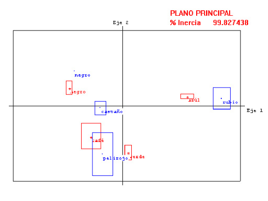
Figure 1: Graph result of the SymCA.