Semi-parametric local variable selection under misspecification

Abstract.

Local variable selection aims to discover localized effects by assessing the impact of covariates on outcomes within specific regions defined by other covariates. We outline some challenges of local variable selection in the presence of non-linear relationships and model misspecification. Specifically, we highlight a potential drawback of common semi-parametric methods: even slight model misspecification can result in a high rate of false positives. To address these shortcomings, we propose a methodology based on orthogonal cut splines that achieves consistent local variable selection in high-dimensional scenarios. Our approach offers simplicity, handles both continuous and discrete covariates, and provides theory for high-dimensional covariates and model misspecification. We discuss settings with either independent or dependent data. Our proposal allows including adjustment covariates that do not undergo selection, enhancing flexibility in modeling complex scenarios. We illustrate its application in simulation studies with both independent and functional data, as well as with two real datasets. One dataset evaluates salary gaps associated with discrimination factors at different ages, while the other examines the effects of covariates on brain activation over time. The approach is implemented in the R package mombf.

Keywords: local null testing, semi-parametric model, Bayesian model selection, Bayesian model averaging, functional data

Local variable selection, or local null hypothesis testing, is a critical issue in many areas of science. In statistical terms, this problem arises in scenarios where researchers are provided with a set of covariates of interest, denoted as $x$, and are tasked with testing whether they have an effect on an outcome $y$, at specific values indicated by additional covariates $z$. For example, consider evaluating whether disparities in salary ($y$) are associated to covariates such as race and gender ($x$) at different career stages ($z$). Although there may be no evidence of such disparities based on race among individuals who have recently entered the workforce (e.g., as a result of newly implemented policies aimed at addressing this matter), there may still exist disparities based on gender and at other career stages. In another application we discuss here, we test whether patient or experiment covariates ($x$) are associated to brain activity ($y$) at various time points ($z$). For a broader discussion and further examples, including both independent and dependent data scenarios, we refer to Paulon et al. (2023). It is important to note that the primary objective in all these examples is testing (multiple) scientific hypotheses indexed by $z$, not merely estimating covariate effects on the outcome. Indeed, our examples illustrate how estimation-focused methods such as tree ensembles, may be prone to considerable false positive inflation.

Semi-parametric models provide a natural framework for analyzing the effect of $x$ at various $z$ to address local variable selection, particularly when the sample size or computational power are not sufficient for the use of fully non-parametric methods, or one wishes to use simpler models to facilitate interpretation. While semi-parametric models are a standard tool for statisticians (e.g., generalized additive models, Cox proportional hazards model), their application to local variable selection has not been extensively studied. Our research primarily contributes in two significant ways. Firstly, we offer a theoretical analysis that highlights a critical potential drawback of standard semi-parametric methods. When the model is even slightly misspecified (as is unavoidable in practice), the type I error of most methods that test a precise null hypothesis converges to 1. This raises a significant concern for local variable selection. Secondly, we propose a strategy to address this pitfall through a simple modification that preserves the interpretability and computational features of semi-parametric models. We give theoretical and empirical evidence that our approach achieves consistent (local) variable selection in scenarios where the model is misspecified. To our knowledge, these results are the first of their kind for high-dimensional local variable selection under misspecification.

Before discussing related literature, Figure 1 illustrates potential issues that arise when the assumed model misspecifies the true mean structure (see Section 5.1 for details). There is a single binary covariate, $x$, defining two groups. The true group means are equal for $z\leq 0$ and different for $z>0$. The goal is to identify the set of $z$’s at which the group means differ, based on $n=100$ observations. Suppose we employ a semi-parametric model based on cubic B-splines, and fit it to the combined data from both groups. The solid black lines in Figure 1 depict the projection of the true group means onto a cubic B-spline basis, i.e. the best approximation that one may recover as $n\rightarrow\infty$. The critical issue emerges when we observe that the projected means are no longer equal for $z\leq 0$ (left panel). As $n$ grows, we will erroneously detect differences between the group means for $z\leq 0$, although truly no differences exist. Here the sample size $n=100$ is moderate and the projected group means are only subtly different for $z<0$, nevertheless this suffices to run into significant type I error issues. Specifically, the right panel shows that a near-one posterior probability is assigned to group differences for $z\in(-1,0)$ (similar issues occur when using posterior intervals or P-values). We note that we employed a moderate number of knots, 20 for the baseline mean and 10 for the group differences. Adding knots as $n$ grows is standard in estimation and forecasting problems and could mitigate type I error inflation. Alas, in our model selection context, the model space size grows exponentially with the number of knots, and the power to detect local differences diminishes. Therefore, it is desirable to have methods that can effectively operate with relatively few knots.

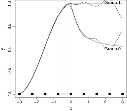
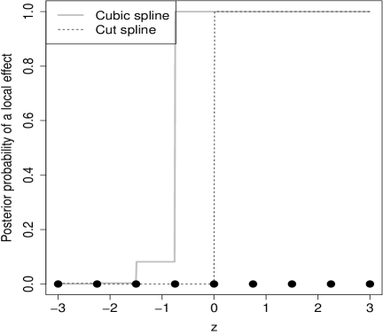
Figure 1. A simulated illustration. True group means and their cubic B-spline projections (left), and posterior probability of local group differences for cubic and cut cubic B-splines based on $n=100$ (right).

This paper considers settings with independent data, where the goal is to perform local variable selection, and some extensions to dependent data. The latter setting received considerable attention in the literature. For instance, Boehm Vock et al. (2015) addressed local variable selection by combining spike-and-slab priors with latent Gaussian processes, an approach extended by Jhuang et al. (2019) using horseshoe priors. Kang et al. (2018) applied a soft-thresholding operator to a Gaussian process for local variable selection. For functional data observed over a common grid (e.g., mass spectrometry, images), Morris et al. (2011) and Zhu et al. (2011) employed basis functions such as wavelets, Fourier transforms, and splines. These methods test whether covariate effects are near 0, rather than exactly 0 as is our goal here. There is also abundant research in settings where $z$ is discrete. For example, Smith and Fahrmeir (2007) proposed a Bayesian framework for regressions on a lattice, whereas Scheel et al. (2013) and Choi and Lawson (2018) focused on variable selection over discrete spatial locations.

A work related to ours is the model by Deshpande et al. (2020) , who employed Bayesian additive regression trees (BART) for varying-coefficient models, both with independent and dependent observations, and established near-minimax estimation rates when the number of covariates grows at a rate slower than $n$. However, their work did not provide theory for variable selection. Furthermore, Paulon et al. (2023) considered a non-parametric framework for time-varying variable selection with discrete covariates, aiming to detect high-order covariate interactions. They established parameter estimation and variable selection consistency for a fixed number of covariates. Here we consider a simpler semi-parametric model that does not require longitudinal data, allows for continuous and discrete covariates and multivariate $z$, and provides high-dimensional theory under model misspecification.

The fundamental aspect of our approach lies in using basis functions that capture covariate effects in a local manner for each neighborhood and are orthogonal to the basis functions used outside that neighborhood. We refer to this construction as an orthogonal cut basis. It can be viewed as an extension of a piece-wise constant parameterization that maintains certain orthogonality properties and allows including higher-degree terms (e.g., cubic terms, as shown in Figure 1). In settings with dependent data, an additional element is required: a block-diagonal approximation to the covariance that captures local dependence. Combined with the orthogonal cut basis, such a purposedly misspecified dependence model ensures consistent local variable selection as $n\rightarrow\infty$.

We set notation. Let $y=(y_{1},\ldots,y_{n})\in\mathbb{R}^{n}$ be the observed outcomes, $x_{i}=(x_{i1},\ldots,x_{ip})$ a vector of $p$ covariates for individual $i$, and $z_{i}\in\mathbb{R}^{d}$ the “coordinates” of interest. In one example $y_{i}$ is the salary of individual $i$ and $z_{i}$ the age, in another $y_{i}$ is the brain activity for a given patient at time $z_{i}$. The goal is to evaluate the effect of $x_{i}$ on $y_{i}$ at each possible $z_{i}$. We remark that our theory and methods also hold when $z_{i}$ is multivariate. However, our examples focus only on univariate $z_{i}$ for simplicity and clarity. Furthermore, effectively deploying the methodology to multivariate functional data in practice requires thorough work in specifying suitable dependence models that falls beyond our scope. Additionally to $z_{i}$, there may be additional adjustment covariates that one includes in the model without undergoing testing. For simplicity we omit said covariates from our exposition, but they are implemented in our software and used in our salary example. We denote the (unknown) data-generating density of $y$ as $F$, which generally lies outside the assumed model class. For purposes of local null testing, it is convenient to partition the support of $z$ into a set of regions $\mathcal{R}=\{R_{1},\ldots,R_{|\mathcal{R}|}\}$ (e.g., the 9 intervals in Figure 1). We will later discuss that one may consider multiple such sets of regions $\mathcal{R}_{1},\ldots,\mathcal{R}_{L}$ and obtain combined inference via Bayesian model averaging. However, for ease of exposition we consider a single $\mathcal{R}$ for now.

The paper is organized as follows. In Section 1, we first discuss a simpler scenario involving a single discrete covariate (group comparisons), which highlights the main issues arising from model misspecification. We then propose a solution based on orthogonal cut bases. In Section 2, we extend these ideas to multiple covariates. Section 3 presents a Bayesian framework for local variable selection, and Section 4 establishes its asymptotic validity. Specifically, we prove that asymptotically one detects which covariates are conditionally uncorrelated with the outcome (given the remaining covariates) at each considered coordinate ($z$), i.e. one attains consistent local variable selection. By Slutsky’s theorem, these results imply that our Bayesian model averaging posterior on the parameters converges to the posterior under the optimal model, where only non-zero parameters are included, hence one also obtains accurate point estimates and asymptotically valid posterior credible intervals. Section 5 shows examples, considering both independent errors and functional data. Finally, Section 6 concludes. The supplementary material contains all proofs, and R scripts to reproduce our analyses. Our methods are implemented in the R package “mombf”.

1. Local variable selection in group comparisons

1.1. Local selection in model-based tests

We consider first the case of a single discrete covariate, $x_{i1}\in\{1,\ldots,K\}$, which defines $K$ distinct groups. Suppose that the true data-generating process, unbeknownst to the data analyst, is characterized by an expectation given by a baseline function $f_{0}(z_{i})$ plus an interaction term $f_{1}(x_{i1},z_{i})$. Specifically, we posit that

(1) $$E_{F}(y_{i}\mid z_{i},x_{i})=f_{0}(z_{i})+f_{1}(x_{i1},z_{i}),\quad i=1,\ldots,n,$$

where $f_{0}$ and $f_{1}$ indicate continuous functions in $z_{i}$. An identifiability condition is required in (1), e.g. a sum-to-zero constraint $\sum_{k=1}^{K}f_{1}(k,z)=0$ at each $z$, so that $f_{1}(k,z)$ represents the deviation from the baseline mean for group $k$ at $z$. The objective of local variable selection is to assess whether the groups have a zero effect at a specific value of $z$, as indicated by the interaction term $f_{1}(k,z)$. This is expressed by the local null hypothesis:

(2) $$f_{1}(1,z)=f_{1}(2,z)=\ldots=f_{1}(K,z)=0.$$

In practice, the true data-generating distribution $F$, as well as the functions $f_{0}$ and $f_{1}$, are unknown and need to be approximated. A common strategy is to model $f_{0}$ and $f_{1}$ using basis functions (such as splines) and to assume a specific error model for the outcome $y=(y_{1},\ldots,y_{n})$, say Gaussian. More specifically, let us consider the approximation of $f_{0}(z_{i})$ with $\beta_{0}(z_{i})=w_{i0}^{T}\eta_{0}$ and $f_{1}(k,z_{i})$ with $\beta_{1k}(z_{i})=w_{ik}^{T}\eta_{1k}$, where $w_{i0}=w_{i0}(z_{i})\in\mathbb{R}^{l_{0}}$ and $w_{ik}=w_{ik}(z_{i})\in\mathbb{R}^{l_{1}}$ evaluate the chosen basis at $z_{i}$ and $(\eta_{0},\eta_{1k})$ denote the corresponding coefficient parameters. Then, (1) is approximated by

(3) $$E_{\eta}(y_{i}\mid z_{i},x_{i1}=k)=\beta_{0}(z_{i})+\beta_{1k}(z_{i})=w_{i0}^{T}\eta_{0}+w_{ik}^{T}\eta_{1k}.$$

Equation (1) describes a so-called varying coefficient model (Hastie and Tibshirani, 1993), where the regression coefficients $\beta_{0}(z_{i})$ and $\beta_{1k}(z_{i})$ depend on $z_{i}$. Assuming Gaussian errors, we can express (3) in matrix notation as:

(4) $$y\mid Z,X\sim N\left(W_{0}\eta_{0}+W_{1}\eta_{1},\Sigma\right),$$

where $W_{0}$ is an $n\times l_{0}$ matrix with $i^{th}$ row given by $w_{i0}$, $W_{1}$ is an $n\times l_{1}K$ matrix with $i^{th}$ row given by $(w_{i1},\ldots,w_{iK})$, and $\Sigma$ represents the error covariance. For instance, one may assume independence and take $\Sigma=\sigma^{2}I$ for some $\sigma^{2}>0$, or consider an appropriate model for dependent data (e.g., autoregressive). To ensure identifiability, we impose an orthogonality constraint $W_{1}^{T}W_{0}=0$ in a manner that $W_{0}\eta_{0}$ represents the baseline mean and $W_{1}\eta_{1}$ represents group deviations from the baseline. This is easily achieved by defining with a standard basis (e.g. splines) and defining $W_{1}$ to be the residuals from regressing that basis onto $W_{0}$, see Section 1.2. For simplicity, we assume that $W$ is non-random, meaning that the covariates $X$ and coordinates $Z$ are fixed, and that any subset of $W$ with $\leq n$ columns has full column-rank.

Under the model specified in (3), the local null hypothesis can be expressed as

(5) $$\beta_{11}(z)=\ldots=\beta_{1K}(z)=0\Longleftrightarrow w_{1}^{T}\eta_{11}=\ldots=w_{K}^{T}\eta_{1K}=0,$$

where $w_{k}=w_{k}(z)$ is the basis function of $\beta_{1k}$ evaluated at a specific $z$. In other words, the local null test at a given $z$ assesses whether a particular linear combination (given by $w_{k}(z)$) of the parameters is zero.

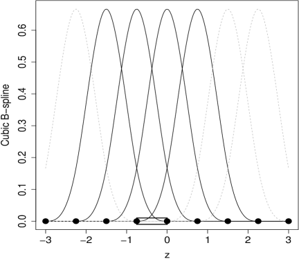
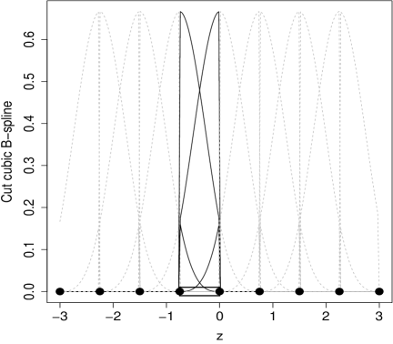
Figure 5. Cubic B-splines (left) and cut cubic B-splines (right) for the simulated illustration in Figure 1.

To facilitate interpretation, we use a local basis such that conducting the test for any $z$ within a given region $R_{b}$ is defined by finding zeroes in $\eta_{1k}$ (rather than in linear combinations $w_{k}(z)^{T}\eta_{1k}$). By a local basis, we mean that the value of $\beta_{1k}(z)$ in each region $R_{b}$ is defined by a small subset of parameters in $\eta_{1k}$. For instance, B-spline bases have minimal support among all spline bases: in an $l$-degree B-spline, each interval between consecutive knots is represented by $l+1$ coefficients. Figure 5 (left) illustrates a cubic B-spline ($l=3$) in which a local hypothesis is tested for $z\in[-0.75,0]$ (black square) with $K=2$ groups. Only $l+1=4$ bases (marked in black) have nonzero values in this interval, specifically bases 2-5. That is, if $\eta_{12}=\eta_{13}=\eta_{14}=\eta_{15}=0$ it then follows that $\beta_{11}(z)=0$ for all $z\in[-0.75,0]$, where we recall that the deviation of group $K=2$ from the baseline is given by $\beta_{12}(z)=-\beta_{11}(z)$, from the identifiability constraint $W_{1}^{T}W_{0}=0$ discussed above.

1.2. Model Misspecification and orthogonal cut basis

One of our main messages is that model-based tests, such as (5), can lead to incorrect conclusions when the mean model is misspecified, i.e. the approximation (4) does not perfectly capture the true mean (1). Under mild conditions, most estimators $\hat{\eta}=(\hat{\eta}_{0},\hat{\eta}_{1})$ for the parameters in Equation (4) converge to the optimal values that minimize the Kullback-Leibler divergence. Consider the independent errors case, with $\Sigma=\sigma I$ in (4). Then, the asymptotically optimal value minimizes mean squared prediction error under the data-generating truth $F$, and is given by a least-squares regression of $E_{F}(y\mid Z,X)$ on $W$,

(6) $$\eta^{*}=\arg\min_{\eta}E_{F}\left[(y-W\eta)^{T}(y-W\eta)\mid Z,X\right]=(W^{T}W)^{-1}W^{T}E_{f}(y\mid Z,X).$$

The issue is that the optimal coefficient values in $\eta^{*}$ associated with a specific region may be non-zero even when the group means are equal in that region. In Figure 1, although the group means are equal for all $z\in[-0.75,0]$, the optimal coefficients $\eta_{12}^{*},\ldots,\eta_{15}^{*}$ associated to this region are non-zero. As $n\rightarrow\infty$, standard frequentist and Bayesian tests provide overwhelming evidence for a group effect at such $z$ values, resulting in false positives. This issue remains problematic even when the sample size is moderate, as in Figure 1 where $n=100$. Intuitively, the issue arises because the coefficients $\eta_{12}^{*},\ldots,\eta_{15}^{*}$ also play a role in approximating the group means outside the region $[-0.75,0]$, e.g. by setting non-zero entries in $\eta_{1}^{*}$ one obtains a better approximation to the true group means for values $z>0$.

To address this issue, we introduce the concept of an orthogonal cut basis. This is a basis for $\beta_{1k}(z)$ that has support only in a region of $z$ values and is orthogonal to bases outside that region. This ensures that the optimal coefficients $\eta_{1}^{*}$ in (6) contain zeroes when there are truly no group differences in a region, e.g. for $z<0$ in Figure 1. This occurs because the cut basis only captures the local effects within the region of interest and does not contribute to approximating the group means outside that region. Figure 5 (right) shows a cut cubic B-spline basis. Specifically, a cut B-spline basis for region $R_{b}$ is equal to the B-spline basis in $R_{b}$ and to 0 outside $R_{b}$. Cut bases, similar to tree-based regression methods, can introduce discontinuities in the estimated group differences. It is important to note that the baseline mean, denoted as $\beta_{0}(z)$, can still be assumed to be continuous. Using B-splines for the baseline mean and cut B-splines for the covariate effects combines desirable features of continuous semi-parametric and discontinuous non-parametric methods.

We next describe orthogonal cut basis more precisely and show that the asymptotic solution $\eta_{1}^{*}$ contains zeroes when there are no local group differences. We partition the support of $z$ into $|\mathcal{R}|$ regions and select a basis $W=(W_{0},W_{1})$ that satisfies two conditions. Let $(y_{b},W_{0b},W_{1b})$ indicate the rows in $(y,\,W_{0},\,W_{1})$ that correspond to the observations in region $b$ (i.e. $z_{i}\in R_{b}$). The first condition is to employ a cut basis $W_{1}$ for group effects $\beta_{1k}(z)$ within each region $b$. This implies that $W_{0}$ and the cut basis $W_{1}$ can be written as

(7) $$W_{0}=\begin{pmatrix}W_{01}\\ W_{02}\\ \ldots\\ W_{0|\mathcal{R}|}\end{pmatrix};\hskip 14.22636ptW_{1}=\begin{pmatrix}W_{11}&0&\ldots&0\\ 0&W_{12}&\ldots&0\\ \ldots&&&\\ 0&0&\ldots&W_{1|\mathcal{R}|}\end{pmatrix}.$$

The second condition is that $W_{1b}$ be orthogonal to $W_{0b}$, i.e. $W_{1b}^{T}W_{0b}=0$, and is satisfied as follows. Let $\widetilde{W}_{1b}$ be a cut basis (e.g. cut B-splines in Figure 1) such that $\widetilde{W}_{1b}^{T}W_{0b}\neq 0$, then we set $W_{1b}=(I-W_{0b}(W_{0b}^{T}W_{0b})^{-1}W_{0b})\widetilde{W}_{1b},$ which are the residuals obtained from regressing $\widetilde{W}_{1b}$ onto $W_{1b}$. Consequently, $W_{1b}^{T}W_{0b}=0$. We refer to any $W_{1}$ satisfying (7) and $W_{1b}^{T}W_{0b}=0$ as an orthogonal cut basis.

Lemma 1 below states that the asymptotic $\eta_{1b}^{*}$, which quantifies the group differences in region $b$, is obtained by regressing the true mean $E_{F}(y_{b}\mid X,Z)$ onto $W_{1b}$ (see Section 7 for the proof). Therefore, if $E_{F}(y_{b}\mid X,Z)$ is not linearly associated with $W_{1}$ in region $b$ (the $K$ data-generating group means are equal in that region), it follows that $\eta_{1b}^{*}=0$.

Lemma 1.

Consider $\eta^{*}=(\eta_{0}^{*},\eta_{1}^{*})$ in (6), where $W=(W_{0},W_{1})$, $W_{0}$ is an $n\times l_{0}$ matrix and $W_{1}$ an $n\times l_{1}$ an orthogonal cut basis as in (7) satisfying $W_{0}^{T}W_{1}=0$. Let $\eta_{1}^{*}=(\eta_{11},\ldots,\eta_{1|\mathcal{R}|}^{*})$ where $\eta_{1b}\in\mathbb{R}^{l_{b}}$ are the parameters associated to $W_{1b}$. Then, $\eta_{1b}^{*}=(W_{1b}^{T}W_{1b})^{-1}W_{1b}^{T}E_{F}(y_{b}\mid X,Z)$.

1.3. Functional data

The presence of dependent observations, as in functional or longitudinal data observed on a dense grid, can introduce additional challenges. More specifically, when assuming a given $\Sigma\neq\sigma^{2}I$, the asymptotic solution becomes

$$\widetilde{\eta}^{*} =\arg\min_{\eta}E_{F}\left[(y-W\eta)^{T}\Sigma^{-1}(y-W\eta)\mid Z,X\right]=(W^{T}\Sigma^{-1}W)^{-1}W^{T}\Sigma^{-1}E_{F}(y\mid Z,X)$$

(8) $$=\eta^{*}+(W^{T}\Sigma^{-1}W)^{-1}W^{T}\Sigma^{-1}\left[E_{F}(y\mid Z,X)-W\eta^{*}\right],$$

where $\eta^{*}$ is defined as in (6). Unless the second term in the right-hand side of (8) is zero, $\tilde{\eta}^{*}$ differs from $\eta^{*}$, meaning that the optimal estimator for independent and dependent data are not equal. Hence, even if $\eta^{*}$ contains zeroes – as guaranteed by Lemma 1 when using orthogonal cut basis – $\tilde{\eta}^{*}$ may not contain zeroes. Intuitively, under correlated errors, the optimal parameters for one region depend on those from the other regions. To address this issue, we employ a block-diagonal approximation for $\Sigma$ that accounts only for within-region dependence. More in detail, we assume that $\Sigma$ is equal to some $\Sigma_{b}$ for observations in region $b$ and 0 elsewhere. We also assume independence across functions, i.e. $\Sigma_{b}$ is also block-diagonal, with blocks corresponding to observations for each individual function. The use of a block-diagonal approximation is reasonable in many functional data applications, as long-range dependence tends to be weak. Related ideas on marginal composite likelihood methods can be found in Caragea and Smith (2006), and Varin et al. (2011) (Section 3.1).

In the case of functional data, assuming that the covariates in $X$ have zero column means, it can be shown that using such a block-diagonal covariance matrix $\Sigma$ leads to an asymptotic $\tilde{\eta}_{1}^{*}$ in (8) that contains zeroes when a covariate has no local effects. The key idea is that Lemma 1 can be extended to $\tilde{\eta}^{*}$ , yielding

$$\tilde{\eta}_{1b}^{*}=(W_{1b}^{T}\Sigma_{b}^{-1}W_{1b})^{-1}W_{1b}^{T}\Sigma_{b}^{-1}E_{F}(y_{b}\mid X,Z).$$

We refer to Lemma 2 for a precise statement. If $E_{F}(y_{b}\mid X,Z)$ does not differ across groups in region $b$ then it is linearly independent of $W_{1b}$ and hence also of $\Sigma_{b}^{-1}W_{1b}$, and then $\tilde{\eta}_{1b}^{*}=0$ by Lemma 2.

In our implementation, we adopt an approximation where we assume a common parametric covariance structure across functions. Based on our experience, this allows for a relatively precise estimation of $\Sigma$. In particular, we propose obtaining $\hat{\Sigma}$ using either a first-order autoregressive or moving average model, selecting the preferred model based on the Bayesian information criterion. Subsequently, we perform inference assuming that $\Sigma=\hat{\Sigma}$ is known. This is convenient in that one can take as a working model

(9) $$\tilde{y}\mid Z,X,\hat{\Sigma}\sim N\left(\widetilde{W}_{0}\eta_{0}+\widetilde{W}_{1}\eta_{1},\sigma^{2}I\right),$$

where $\tilde{y}=\hat{\Sigma}^{-1/2}y$, $\widetilde{W}_{0}=\hat{\Sigma}^{-1/2}W_{0}$ and $\widetilde{W}_{1}=\hat{\Sigma}^{-1/2}W_{1}$. This representation enables us to readily apply standard Bayesian independent errors calculations on $\tilde{y}$, including model search and posterior sampling strategies. We note that our theoretical framework and methodology are applicable to scenarios involving multivariate $Z$. However, effectively implementing the approach in a multivariate context would likely require alternatives to the auto-regressive and moving average models we employ here. Therefore, exploring these alternatives and their implementation is left as future work.

2. Extension to multiple covariates

We extend our approach to settings involving a covariate vector $x_{i}=(x_{i1},\ldots,x_{ip})$. In this case, the data-generating truth in (1) is expanded to $E(y_{i}\mid z_{i},x_{i})=f_{0}(z_{i})+f_{1}(x_{i},z_{i})$. Similar to (1), we consider an identifiability constraint so that $f_{0}(z_{i})$ represent the baseline mean and $f_{1}(x_{i},z_{i})$ represents deviations from the mean. Therefore, the local null test for covariate $j$ at $z$ corresponds to assessing whether $f_{1}(x_{i},z)=0$ depends on $x_{ij}$ or not. To impose this constraint, we orthogonalize the basis used for $f_{1}$ with respect to that for $f_{0}$, as explained below.

As previously discussed in relation to (3), model-based approaches for local variable selection involve approximating $(f_{0},f_{1})$ using a suitable function class and then expressing the selection in terms of the parameters of that class. While it is possible to model $f_{1}(x,z)$ non-parametrically, and assess the effect of $x$ at each given $z$, the computational burden increases sharply as $p$ or the number of possible $z$ values increase (the model space grows exponentially with the number of parameters). Instead, we consider a semi-parametric model that assumes additive covariate effects,

(10) $$E_{\eta}(y_{i}\mid z_{i},x_{i})=\beta_{0}(z_{i})+\sum_{j=1}^{p}\,\beta_{1j}(z_{i})x_{ij}=w_{i0}^{T}\eta_{0}+\sum_{j=1}^{p}\,w_{ij}^{T}\eta_{1j}.$$

Analogously to (3), $\beta_{0}(z_{i})=w_{i0}^{T}\eta_{0}$ approximates $f_{0}(z_{i})$, $x_{ij}\beta_{1j}(z_{i})=w_{ij}^{T}\eta_{1j}$ provides an additive approximation to $f_{1}(x_{i},z_{i})$, $w_{i0}=w_{i0}(z_{i})\in\mathbb{R}^{l_{0}}$ and $w_{ij}=w_{ij}(z_{i})\in\mathbb{R}^{l_{1}}$ are basis expansions computed from $(z_{i},x_{i})$, and $(\eta_{0},\eta_{11},\ldots,\eta_{1p})\in\mathbb{R}^{l_{0}+l_{1}p}$ are the corresponding parameters. We denote the total number of parameters as $q=l_{0}+l_{1}p$.

Note that the expectation $E_{F}(y_{i}\mid z_{i},x_{i})$ under the data-generating truth $F$ may not be additive, e.g. the effect of covariate $j$ at $z$ may interact with that of covariate $j^{\prime}$. However, the parameters in the assumed model (10) remain interpretable, e.g. $\beta_{1j}(z)$ is the mean effect of covariate $j$ at coordinate $z$, averaged across the values of other covariates. Hence, even in the face of potential model misspecification, testing whether $\beta_{1j}(z)=0$ remains a sensible goal. Note also that if desired one may relax the additivity assumption, e.g., by incorporating interactions and tensor products, and define $w_{i}$ to be the vector containing all such terms. However we do not pursue that here, rather we focus on providing a model that tests for average local effects and remains easy to interpret.

Assuming a Gaussian distribution for $y$, (10) can be written as

(11) $$y\mid Z,X\sim N(W_{0}\eta_{0}+W_{1}\eta_{1},\Sigma),$$

where $\Sigma$ is as in (4) and $(W_{0},W_{1})$ is an orthogonal cut basis as in (7). The only difference relative to (7) is that we extend $W_{1b}$, the basis for local covariate effects, by multiplying it by the value of each covariate (akin to interaction terms in standard regression). For brevity we omit details, which are provided in Section 8. There we also discuss that, since $W_{1}$ is an orthogonal cut basis, Lemmas 1 and 2 still apply: if $E_{F}(y_{b}\mid X,Z)$ is linearly independent of covariate $j$ given the other covariates, then the asymptotic covariate effect in region $b$ is $\eta_{1jb}^{*}=0$ (for dependent data, $\tilde{\eta}_{1jb}^{*}=0$).

As a practical remark, although our discussion applies to generic basis functions that can be quite flexible, such as cubic splines, the computational burden can become substantial when dealing with many covariates. In our examples, we found that using cubic splines for defining the baseline ($W_{0}$) and 0-degree splines for the local covariate effects led to faster computations without compromising the quality of inference for local variable selection.

3. A framework for local null testing

Equation (11) defines the likelihood associated to the observed $y\in\mathbb{R}^{n}$, given the design matrices $W_{0},W_{1}$ constructed from the $p$ covariates in $X$, the coordinates in $Z$, and the corresponding parameters $\eta=(\eta_{0},\eta_{1})\in\mathbb{R}^{l_{0}+l_{1}p}$. As described in (18), under model (11), testing for the effect of covariate $j=1,\ldots,p$ in region $b\in\{1,\ldots,|\mathcal{R}|\}$ is equivalent to testing $\eta_{1jb}=0$ versus $\eta_{1jb}\neq 0$, resulting in a total of $p|\mathcal{R}|$ tests. Section 3.1 below discusses how to incorporate these tests into a standard Bayesian model selection framework. Section 3.2 proposes default priors. In Section 3.3, we explore an alternative approach where instead of pre-defining a fixed set of regions, multiple resolutions are considered. These resolutions can be combined using Bayesian model averaging, providing flexibility and adaptability in capturing the underlying structure of the data.

3.1. Bayesian model selection and averaging

In order to describe any arbitrary model within the local variable selection process, we introduce latent variables $\gamma=\{\gamma_{jb}\}$, where $\gamma_{0b}=\mbox{I}(\eta_{0b}\neq 0)$ and $\gamma_{jb}=\mbox{I}(\eta_{1jb}\neq 0)$ serve as indicators for variable inclusion across regions $b=1,\ldots,|\mathcal{R}|$ and covariates $j=1,\ldots,p$. The model size, i.e. the number of non-zero parameters, is denoted as $|\gamma|_{0}=\sum_{jb}\gamma_{jb}$.

The goal is to select the optimal model $\gamma^{*}$, where $\gamma_{jb}^{*}=\mbox{I}(\eta_{1jb}^{*}\neq 0)$, with $\eta^{*}$ minimizing the mean squared prediction error under the data-generating truth $F$ in (6) and (8). When considering model misspecification, $\gamma^{*}$ represents the optimal model among those under consideration. Specifically, it is the model with the smallest dimension $|\gamma^{*}|_{0}$ among those that are Kullback-Leibler closest to $F$ (see Rossell (2022)).

The posterior probability of model $\gamma$ is obtained as

(12) $$p(\gamma\mid y)=\frac{p(y\mid\gamma)\,p(\gamma)}{p(y)}=\frac{p(\gamma)\int p(y\mid\eta)\,p(\eta\mid\gamma)\,d\eta}{p(y)},$$

where $p(\gamma)$ indicates the model’s prior probability and $p(\eta\mid\gamma)$ the prior on the parameters under model $\gamma$ (see Section 3.2). Given the posterior distribution $p(\gamma\mid y)$ for the entire vector $\gamma$, one can assess the local effect of covariate $j$ in region $b$ using the marginal posterior inclusion probabilities

(13) $$P(\gamma_{jb}=1\mid y)=\sum_{\gamma:\gamma_{jb}=1}\,p(\gamma\mid y).$$

As shown in Section 4, under mild regularity conditions, $p(\gamma^{*}\mid y)$ converges to 1 as $n$ grows, and thus (13) concentrates on $\gamma^{*}_{jb}$ uniformly across the pairs $(j,b)$. This guarantees that, for sufficiently large $n$, using either (12) or (13) leads to consistently selecting $\gamma^{*}$ and vanishing family-wise type I-II error rates.

We propose including local covariate effects that have high marginal posterior probability in (13). Specifically, we set $\hat{\gamma}_{j}=P(\gamma_{jb}=1\mid y)\geq t$, for some threshold $t\in(0,1)$. In our illustrations, we used $t=0.95$. This choice ensures that the model-based posterior expected false discovery proportion (FDP) remains below 0.05, see Müller et al. (2004). We point out that this procedure also has a connection with frequentist type I errors. According to Corollary 2 in Rossell (2022), for any true $\gamma^{*}_{jb}=0$, the frequentist probability of falsely selecting a covariate $j$ in region $b$ under any data-generating $F$ is upper bounded by $P_{F}(\hat{\gamma}_{jb}=1)\leq t^{-1}E_{F}\left[P(\gamma_{jb}=1\mid y)\right]$.

3.2. Priors for the local effects and model selection

Posterior model probabilities in (12) require setting a prior $p(\gamma)$ on the models and a prior $p(\eta_{\gamma}\mid\gamma)$ on the coefficients under each model. For the latter, we consider a Normal shrinkage prior

(14) $$p(\eta_{\gamma}\mid\gamma)=N\left(\eta_{\gamma};0,g\,\mbox{diag}(W_{\gamma}^{T}W_{\gamma}/n)^{-1}\right)$$

where $g>0$ is a prior dispersion parameter. By default, we set $g=1$ so that the trace of the prior precision equals that of the unit information prior of Schwarz (1978). Note that (14) can be viewed a imposing a penalty on the $L_{2}$ norm of $\eta$, and that our multi-resolution analysis (Section 3.3) encourages smoothness across coordinates $Z$ in the fitted regression. Although we focus our discussion on (14), in settings with very strong dependence and moderate $n$, we found that replacing (14) by a group pMOM prior with default parameters (Rossell et al. (2021)) helped prevent type I error inflation. Therefore, for dependent data, we recommend the group pMOM prior as the default choice (see Sections 5.2 and 5.4 for examples).

For the model prior, we consider a Complexity prior akin to Castillo et al. (2015),

(15) $$p(\gamma)=\frac{C}{q^{c|\gamma|_{0}}}\times{q\choose|\gamma|_{0}}^{-1}\mbox{I}(|\gamma|_{0}\in\{0,\ldots,\bar{q}\}),$$

where recall that $q$ is the total number of parameters defined after (10), $c\geq 0$ a prior parameter, $C=[1-1/q^{c}]/[1-1/q^{c*(\bar{q}+1)}]$ the normalizing constant, and we consider that, although possibly $q\gg n$, one restricts attention to models with $|\gamma|_{0}\leq\bar{q}$ parameters, where $\bar{q}$ is a user-defined bound such as $\bar{q}\leq n$ (since models with $|\gamma|_{0}>n$ result in data interpolation). For $c>0$ the prior probabilities decay exponentially with the model size, $|\gamma|_{0}$, and then equal prior probabilities are set on all models that have the same size.

Setting $c=0$ returns the Beta-Binomial(1,1) prior of Scott and Berger (2006), i.e. a uniform prior on the model size, which served as the basis for the extended BIC of Chen and Chen (2008). Indeed, while our primary emphasis is on Bayesian methods, the theoretical results shown in Section 4 can be seamlessly adapted to the extended BIC framework by setting $c=0$ and $g=1$. In our theoretical framework, we consider a general value for $c$. However, in our practical examples we set $c=0$, since for finite $n$ in on our experience this yields a better balance between sparsity and power to detect non-zero coefficients.

3.3. Multi-resolution analysis

So far, to simplify exposition, we assumed that a predefined set of regions $\mathcal{R}$ is used for performing the local null tests, such as the 8 intervals shown in Figure 1. In practice, it is often unclear what regions to use, or in other words, what resolution is appropriate for the local variable selection. To illustrate this point, consider a scenario where there is a single binary covariate $x_{i}$ that defines two groups, and we are interested in comparing $E(y_{i}\mid z_{i},x_{i})$ across these groups. If the group differences remain roughly constant across large regions in $z_{i}$, it would be advantageous to use a coarse resolution with fewer regions, to increase statistical power. In contrast, if the group differences change rapidly with $z_{i}$, a finer resolution with more regions may be preferred, for capturing local variations and detecting smaller-scale differences between the groups. In practice, the choice of the maximum number of regions is typically guided by computational limitations (as the model space grows exponentially) or because higher resolutions offer limited practical interest. A multi-resolution analysis is instrumental in determining if a coarser resolution might be more suitable. For example, in our salary application, we consider 2.5- year bins as the highest resolution, since policies or other measures targeting salary discrimination are unlikely to have noticeable effects in shorter time spans. Interestingly, our multi-resolution analysis places most posterior probability on (coarser) 5-year intervals. See Section 5.4 for a related discussion on our brain data.

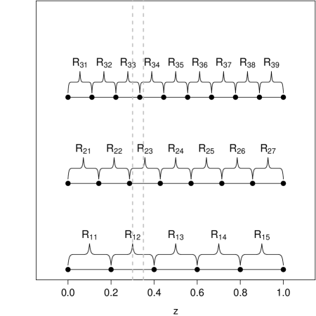
Figure 2. Multi-resolution analysis: an illustration considering 3 resolution levels with $z\in[0,1]$, defining 5, 7 and 9 regions respectively. If we focus on resolutions 1-2, one can note that $\beta_{j}(z=0.3)\neq 0$ if and only if $\beta_{j}(z=0.35)\neq 0$ (dashed lines), leading to prior dependence across $z$. See Section 3.3 for details.

Bayesian model averaging provides a natural framework for considering multiple resolution levels. We consider $L$ resolutions, where each resolution $l=1,\ldots,L$ consists of a set of regions $\mathcal{R}_{l}={R}_{l1},\ldots,R_{l|\mathcal{R}_{l}|}$. An example with three resolutions and their corresponding regions is shown in Figure 2. Similar to Section 3.2, let $\eta_{l}=\{\eta_{ljb}\}$ and $\gamma_{l}=\{\gamma_{ljb}\}$ for $j=0,\ldots,p$ and $b=1,\ldots,|\mathcal{R}_{l}|$ represent the set of parameters and models associated with resolution $l$, where the latent $\gamma_{ljb}=\mbox{I}(\eta_{lbj}\neq 0)$ indicates whether covariate $j$ has an effect in region $R_{lb}$. We consider a joint prior that factorizes as follows,

$$p(\eta_{l},\gamma_{l},\mathcal{R}_{l})=p(\eta_{l}\mid\gamma_{l},\mathcal{R}_{l})\,p(\gamma_{l}\mid\mathcal{R}_{l})\,p(\mathcal{R}_{l}).$$

where $p(\eta_{l}\mid\gamma_{l},\mathcal{R}_{l})$ is as in (14), and the model selection prior in (15) is modified to accommodate the multi-resolution setting as follows,

(16) $$p(\gamma_{l}\mid\mathcal{R}_{l})=\frac{C_{l}}{q_{l}^{c|\gamma|_{0}}}\times{q_{l}\choose|\gamma_{l}|_{0}}^{-1}\mbox{I}(|\gamma_{l}|_{0}\in\{0,\ldots,\bar{q}\}),$$

where $q_{l}=\mbox{dim}(\eta_{l})$ is the number of parameters for resolution $l$, $c\geq 0$ and $C_{l}=[1-1/q_{l}^{c}]/[1-1/q_{l}^{c*(\bar{q}+1)}]$ the normalizing constant. Finally, by default, uniform prior probabilities are assigned to the resolution levels, i.e., $p(\mathcal{R}_{l})=1/L$.

The multi-resolution formulation induces dependence in the local variable selection across nearby $z$ values, as illustrated in Figure 2. Specifically, the probability of a local effect is $P\left(\beta_{j}(z)\neq 0\right)=\sum_{l=1}^{L}P\left(\beta_{j}(z)\neq 0\mid\mathcal{R}_{l}\right)p(\mathcal{R}_{l})$, where $P\left(\beta_{j}(z)\neq 0\mid\mathcal{R}_{l}\right)$ is constant across all $z$ values within the same interval at resolution $l$. Hence, nearby $z$ and $z^{\prime}$ receive similar prior probabilities $P(\beta_{j}(z)\neq 0)$ and $P(\beta_{j}(z^{\prime})\neq 0)$. The corresponding posterior probabilities are

$$P\left(\beta_{j}(z)\neq 0\mid y\right) =\sum_{l=1}^{L}P\left(\beta_{j}(z)\neq 0\mid y,\mathcal{R}_{l}\right)\,p(\mathcal{R}_{l}\mid y),$$

where $P\left(\beta_{j}(z)\neq 0\mid\mathcal{R}_{l},y\right)$ given a resolution level $l$ is given in (13), and $p(\mathcal{R}_{l}\mid y)\propto p(y\mid\mathcal{R}_{l})\,p(\mathcal{R}_{l})=\sum_{\gamma_{l}}p(y\mid\gamma_{l},\mathcal{R}_{l})p(\gamma_{l}\mid\mathcal{R}_{l})\,p(\mathcal{R}_{l})$ is the marginal likelihood of resolution $l$.

We remark that our multi-resolution strategy is designed to facilitate parallel computation across different resolutions. We define a distinct model for each resolution $\mathcal{R}_{l}$, obtain $P(\beta_{j}(z)\neq 0\mid y,\mathcal{R}_{l})$ separately for each resolution, and then compute their weighted average. A natural alternative would involve inducing prior dependence across resolutions. This is because, if for example $\beta_{j}(z)=0$ for all $z$ at a certain resolution, then $\beta_{j}(z)=0$ also holds true at any coarser resolution. However, we chose not to adopt such more advanced priors here. The primary reason is that computations would no longer be easily parallelizable. Moreover, in our examples, our simpler prior proved sufficiently effective.

4. Theoretical results

We present two main results describing the asymptotic behavior of the proposed cut basis framework. First, we obtain rates at which the Bayes factor favors the optimal model $\gamma^{*}$ over some other model $\gamma$ (Theorem 1). Then, we establish that the posterior model probabilities consistently select $\gamma^{*}$ (Theorem 2). These results imply that asymptotically one detects which covariates have an effect at each considered coordinate $z$, and hence attains consistent local variable selection. As discussed in Section 2, since the assumed additive structure in (10) may be misspecified, consistency refers to detecting non-zero marginal effects of each covariate in $x$, averaged across the values of other covariates in $x$. We consider high-dimensional settings where the total number of parameters $q=l_{0}+l_{1}p$ can grow with $n$. The size of the optimal model $|\gamma^{*}|$ may also increase with $n$.

We assume that the data-generating $F$ has sub-Gaussian tails, specifically $F$ satisfies $y-W_{\gamma^{*}}\eta_{\gamma^{*}}^{*}\sim SG(0,\omega)$ for some $\omega>0$. This assumption allows for $y$ to be dependent. For example, if $y\sim N(\mu,\Omega)$ for some positive-definite $\Omega$, then $y\sim SG(\mu,\omega)$ where $\omega$ is the largest eigenvalue of $\Omega$. We consider a misspecified setting where the data analyst specifies a model that may not match $F$. To simplify the exposition and proofs, we assume that the specified model has a fixed covariance, $\Sigma$. Specifically, data analyst specifies the model

(17) $$\begin{split}y\mid\gamma,\eta_{\gamma}&\sim N(W_{\gamma}\eta_{\gamma},\Sigma)\\ \eta_{\gamma}\mid\gamma&\sim N(0,gV_{\gamma}),\end{split}$$

where $V_{\gamma}$ is a $|\gamma|_{0}\times|\gamma|_{0}$ positive-definite matrix, and $g\in\mathbb{R}^{+}$. We recall that, when the columns in $W$ have zero sample mean and unit variance, in our default choice for the prior in (14), we set $V_{\gamma}=I$ and $g=1$, which is a minimally informative prior. Our theory allows for other $g$ and $V_{\gamma}$, e.g. letting $g$ grow with $n$ to enforce sparsity, at the cost of decreased statistical power, see Narisetty and He (2014); Rossell (2022) for further discussion.

4.1. Bayes factors

The Bayes factor $B_{\gamma\gamma^{*}}=p(y\mid\gamma)/p(y\mid\gamma^{*})$ compares a model $\gamma$ with the optimal $\gamma^{*}$, see Section 10 for its expression, such that when $B_{\gamma\gamma^{*}}$ is close to zero then $\gamma^{*}$ is favored over $\gamma$. We give the rates at which $B_{\gamma\gamma^{*}}$ converges to 0 in probability as $n\rightarrow\infty$, assuming the following regularity conditions.

1. The matrix $W_{\gamma}^{T}\Sigma^{-1}W_{\gamma}$ has full column rank $|\gamma|_{0}$.

2. Let $(\underline{l}_{\gamma},\bar{l}_{\gamma})$ be the smallest and largest eigenvalues of $V_{\gamma}W_{\gamma}^{T}\Sigma^{-1}W_{\gamma}/n$. They satisfy $c_{1}\leq\underline{l}_{\gamma}\leq\bar{l}_{\gamma}\leq c_{2}$ for all $n\geq n_{0}$ and some constants $c_{1},c_{2},n_{0}>0$.

3. $\Sigma^{-1}$ exists. Its largest eigenvalue $\tau$ satisfies $c_{3}<\tau<c_{4}$ for constants $0<c_{3},c_{4}<\infty$.

4. $\lim_{n\rightarrow\infty}gn=\infty$.

5. Let $\lambda_{\gamma}=(\widetilde{W}_{\gamma^{*}}\eta_{\gamma^{*}}^{*})^{T}(I-H_{\gamma})\widetilde{W}_{\gamma^{*}}\eta_{\gamma^{*}}^{*}$, where $\widetilde{W}_{\gamma}=\Sigma^{-1/2}W_{\gamma}$, $H_{\gamma}=\widetilde{W}_{\gamma}(\widetilde{W}_{\gamma}^{T}\widetilde{W}_{\gamma})^{-1}\widetilde{W}_{\gamma}^{T}$. For some sequence $d_{n}\geq 0$ such that $\lim_{n\rightarrow\infty}d_{n}=\infty$,

   $$\lim_{n\rightarrow\infty}\frac{\lambda_{\gamma}}{2\log\lambda_{\gamma}}+\frac{|\gamma|_{0}-|\gamma^{*}|_{0}}{2}\log(gn)-\omega\tau|\gamma|_{0}\log d_{n}=\infty.$$

The conditions are fairly minimal, for brevity we refer their discussion to Section 11. A key quantity is $\lambda_{\gamma}$ in Assumption (A5), it is a non-centrality parameter measuring the sum of squares explained by the optimal $\gamma^{*}$ but not by model $\gamma$. Under eigenvalue and beta-min conditions, $\lambda_{\gamma}$ is lower-bounded by $n$ times the smallest square entry in the optimal coefficients $|\eta_{\gamma^{*}}^{*}|$ (see, e.g., Rossell, 2022, Sections 2.2 and 5.4).

Before stating Theorem 1, we interpret its main implications. Part (i) indicates that overfitted models, which include all parameters in $\gamma^{*}$ and some extra, are essentially discarded at a polynomial rate $(gn)^{(|\gamma|_{0}-|\gamma^{*}|_{0})/2}$. Part (ii) states that non-overfitted models, which are missing parameters from $\gamma^{*}$, are effectively discarded at an exponential rate in $\lambda_{\gamma}$, times a polynomial rate akin to that in Part (i). In the theorem statement the sequence $d_{n}$ should be considered as a lower-order term, e.g., $d_{n}=\log(gn)$, and $\delta$ as a constant close to 0.

Theorem 1.

Let $d_{n}\geq 0$ be any sequence such that $\lim_{n\rightarrow\infty}d_{n}=\infty$. Assume (A1)-(A5).

1. Overfitted models. If $\gamma^{*}\subset\gamma$, then $\lim_{n\rightarrow\infty}P_{F}\left(B_{\gamma\gamma^{*}}\geq\left(\frac{d_{n}}{gn}\right)^{\frac{|\gamma|_{0}-|\gamma^{*}|_{0}}{2}}\right)=0.$

2. Non-overfitted models. If $\gamma^{*}\not\subset\gamma$, then for all fixed $\delta>0$

   $$\lim_{n\rightarrow\infty}P_{F}\left(B_{\gamma\gamma^{*}}\geq\left(gnk_{2}\right)^{-\frac{(|\gamma|_{0}-|\gamma^{*}|_{0})}{2}}e^{-\frac{\lambda_{\gamma}(1-\delta)}{2\log\lambda_{\gamma}}+\omega\tau|\gamma|_{0}\log d_{n}}\right)=0,$$

   where $\omega$ is the sub-Gaussian parameter, $\tau$ the largest eigenvalue of $\Sigma^{-1}$ and $k_{2}=\bar{l}_{\gamma^{*}}(1+\delta)/\underline{l}_{\gamma}$ is a constant under Assumption (A2).

4.2. Model selection consistency

Theorem 2 below shows that the posterior probability of the optimal model $p(\gamma^{*}\mid y)\stackrel{{\scriptstyle L_{1}}}{{\longrightarrow}}1$ as $n\rightarrow\infty$ and provides the associated rate. The result bounds separately the total posterior probability assigned to the set of overfitted models ($S_{0}$), and to non-overfitted models that are either smaller ($S_{1}$) or larger ($S_{2}$) than the optimal $\gamma^{*}$. This decomposition helps understand false positive versus power trade-offs.

Theorem 2 requires additional conditions involving the sub-Gaussian parameter $\omega$ of the data-generating $F$, the largest eigenvalue $\tau$ of $\Sigma^{-1}$, the prior dispersion parameter $g$ in (14), and the model prior parameter $c\geq 0$ in (15). More specifically,

1. The optimal model has size $|\gamma^{*}|_{0}\leq\bar{q}$, where $\bar{q}$ is the maximum model size in (15).

2. $\omega\,\tau>1$.

3. $p(\gamma)$ is non-increasing in model size $|\gamma|_{0}\in\{0,\ldots,\bar{q}\}$ and, for any $|\gamma|_{0}>|\gamma^{*}|_{0}$,

   $$\lim_{n\rightarrow\infty}\frac{1}{2}\log(gn)+\frac{1}{|\gamma|_{0}-|\gamma^{*}|_{0}}\log\left(\frac{p(\gamma^{*})}{p(\gamma)}\right)-(1+\sqrt{2})^{2}\omega\tau\bar{q}=\infty.$$

4. For some $a\in(0,1/[2\omega\tau])$, $\lim_{n\rightarrow\infty}a\log(gn)+a(c+1)\log(q)-\log(q)=\infty.$

5. For any not over-fitted model $\gamma\not\subset\gamma^{*}$ of size $|\gamma|_{0}\leq|\gamma^{*}|_{0}$ and any fixed $k>0$,

   $$\lim_{n\rightarrow\infty}t+\frac{\lambda_{\gamma}}{\log\lambda_{\gamma}}-k|\gamma|_{0}\log\left(t+\frac{\lambda_{\gamma}}{\log\lambda_{\gamma}}\right)=\infty$$

   where $t=(|\gamma|_{0}-|\gamma^{*}|_{0})\log(gn\,k_{2})+2\log\left(p(\gamma^{*})/p(\gamma)\right).$

6. Let $\underline{\lambda}=\frac{\min_{|\gamma|_{0}\leq|\gamma^{*}|_{0}}\lambda_{\gamma}}{\max\{|\gamma^{*}|_{0}-|\gamma|_{0},1\}}$. Then, $\lim_{n\rightarrow\infty}\frac{\underline{\lambda}}{2\omega\tau}-c\log(q)-\frac{1}{2}\log(gn)=\infty.$

7. For some $r<1/[\omega\,\tau]$, $\lim_{n\rightarrow\infty}\frac{(|\gamma^{*}|_{0}+1)\bar{q}^{r}}{q^{cr-1-|\gamma^{*}|_{0}}(q-|\gamma^{*}|_{0})^{r}(gn)^{r/2}}=0$.

Assumption (B1) says that the optimal model $\gamma^{*}$ has positive prior probability. Assumption (B2) is a worst-case scenario, one obtains faster rates in Theorem 2(i) and (iii) if $\omega\tau<1$, see the proof for details. Assumption (B3) is a mild requirement that $g\,n$ and $p(\gamma^{*})/p(\gamma)$ are not too small relative to the model size $|\gamma|_{0}$. (B4) bounds the total number of parameters $q$ as a function of $n$, and is satisfied by setting a large $c$ (sparse model prior) or $g$ (dispersed coefficient prior). Assumptions (B5) and (B6) are stronger versions of (A5) requiring that the non-centrality parameters $\lambda_{\gamma}\geq(|\gamma^{*}|_{0}-|\gamma|_{0})\underline{\lambda}$ are large enough. Altogether, (B4)-(B6) limit the amount of prior sparsity induced by the model prior parameter $c$ and the prior dispersion $g$, relative to $n$ and $q$. Finally, Assumption (B7) is similar to (B2)-(B3) and ensures that the rate in Theorem 2(iii) converges to 0. (B7) is stronger than needed but simplifies the exposition, please see Assumption (B7’) and Theorem 3 in Section 16 for further details.

Theorem 2.

1. Assume (A1)-(A5) and (B2)-(B4). Let $S_{0}=\{\gamma:\gamma^{*}\subset\gamma\}$. There exist constants $k>0$ and $n_{0}$ such that, for all $n\geq n_{0}$ and $r<1/[\omega\tau]$,

   $$E_{F}(P(S_{0}\mid y))<\frac{k(|\gamma^{*}|_{0}+1)}{q^{r(c+1)-1}(gn)^{\frac{r}{2}}}.$$

2. Assume (A1)-(A5), (B1), (B2), (B5) and (B6). Let $\underline{\lambda}$ be the signal strength parameter in (B6), and $S_{1}=\{\gamma:|\gamma|_{0}\leq|\gamma^{*}|_{0},\gamma\not\subset\gamma^{*}\}$. For $n\geq n_{0}$ and fixed $n_{0}$,

   $$E_{F}(P(S_{1}\mid y))<9\exp\left\{-\frac{\underline{\lambda}(1-\epsilon)}{2\tilde{\omega}}+[|\gamma^{*}|_{0}(1+\epsilon)+c]\log q+\frac{1}{2}\log(gn)\right\},$$

   for a constant $\alpha>0$ that may be taken arbitrarily close to 0.

3. Assume (A1)-(A5), (B1), (B2), (B5) and (B7). Let $S_{2}=\{\gamma:|\gamma|_{0}>|\gamma^{*}|_{0},\gamma\not\subset\gamma^{*}\}$. There exist constants $k>0$ and $n_{0}$ such that, for all $n\geq n_{0}$ and $r<1/[\omega\tau]$,

   $$E_{F}(P(S_{2}\mid y))\leq\frac{k(|\gamma^{*}|_{0}+1)b^{1/2}\bar{q}^{r}}{q^{cr-1-|\gamma^{*}|_{0}}(q-|\gamma^{*}|_{0})^{r}(gn)^{r/2}}.$$

In Theorem 2, $r$ should regarded as being close to $1/[\omega\,\tau]$. Theorem 2 (i) and (iii) state that overfitted and large non-overfitted models (respectively) receive vanishing posterior probability as $n$ grows, at a rate that is faster when the prior complexity and the dispersion parameters $(c,g)$ are large, and slower when either the optimal model is not sparse (i.e., $|\gamma^{*}|_{0}$ is large) or $\omega\tau$ is large. In the well-specified case where $F$ is Gaussian with independent observations, then $\omega\,\tau=1$. Hence, the condition $r<1/[\omega\,\tau]<1$ reflects that under strongly dependent data or model misspecification, convergence rates get slower. Similarly, Part (ii) states that small non-overfitted models are discarded at an exponential rate in $\underline{\lambda}/[2\omega\,\tau]$, which gets slower when $\omega\,\tau>1$ and when either $q$ or $|\gamma^{*}|_{0}$ are large. Note that if $(c,g)$ are large, i.e. chosen to favor smaller models, then the convergence rate is slower. This reflects the intuitive notion that, by inducing stronger sparsity, the statistical power to detect truly active coefficients is reduced.

5. Empirical illustration

We assess the performance of our framework through simulations and two examples. Section 5.1 considers a simulation with independent errors to compare our cut orthogonal basis with standard (uncut) cubic splines, the VC-BART of Deshpande et al. (2020) for fitting a varying coefficient model using Bayesian additive regression trees, and a least-squares regression where one obtains Benjamini-Hochberg adjusted P-values for interactions between each covariate and discretized coordinates $z$. Section 5.2 extends the simulations to functional data with highly dependent errors. Here, we compare our approach to the LFMM method of Paulon et al. (2023) and to the interval testing procedure of Pini and Vantini (2016). The latter is designed for a single covariate and the former is designed to detect high-order interactions between multiple discrete covariates. Finally, Section 5.3 analyzes a salary survey data from independent individuals, and Section 5.4 considers functional data from a neuroscience experiment.

For our methodology, we used a cubic B-spline with 20 knots for the baseline and a multi-resolution analysis involving 7, 9 and 11 knots to evaluate the covariate effects. We considered cut basis of degree 0 (piecewise-constant) and 3 (cubic) but we only report the results from the former, since the results were very similar. Following our previous discussion, we used the Gaussian shrinkage prior (14) for the independent error settings, whereas we used the group product moment prior of Rossell et al. (2021) for functional data, in both cases with default parameters. For our computations, we used Markov Chain Monte Carlo sampling to search over models characterized by different $\gamma$, and to obtain posterior probability estimates for the covariate effects as well as posterior samples for all the model parameters. For this purpose, we used the default specifications in the R package mombf (10,000 Gibbs iterations, with 500 burn-in). Since these are standard MCMC algorithms we do not outline them here for brevity, and refer the reader to Rossell and Telesca (2017).

5.1. Simulation with independent errors

We illustrate the issues that may arise when employing a standard cubic B-splines for local variable selection, and how these issues are addressed by using a cut orthogonal basis. We consider two scenarios, with $n=100$ and $n=1,000$. In both cases, we consider $p=10$ covariates, and a regular grid of $n$ values for $z_{i}\in[-3,3]$. The first covariate is a binary group indicator $x_{i1}\in\{0,1\}$ with equal group sizes. The remaining covariates are generated from a normal distribution with mean $x_{i1}$, and variance 1, $x_{ij}\sim N(x_{i1},1)$. This results in a mild empirical correlation between $x_{1}$ and each remaining covariate of 0.43. The expected outcome is set to depend truly only on the first covariate, and that only when $z>0$, as depicted in Figure 1 (grey lines). More in detail, we set the following model

$$E(y_{i}\mid x_{i},z_{i})=\begin{cases}\cos(z_{i}),&\mbox{ if }z_{i}\leq 0,\\ 0,&\mbox{ if }z_{i}>0,x_{i1}=1,\\ 1/(z_{i}+1)^{2},&\mbox{ if }z_{i}>0,x_{i1}=0,\end{cases}$$

We consider 100 independent replicates of each scenario.

Table 2 shows the type I error and power for the cut and standard B-spline basis, and for the Benjamini-Hochberg P-value adjusted method. The latter exhibits a low type I error, but the power is very low for small $n$. For example, for $n=100$ and $z\in(1,2]$, the estimated power for covariate 1 is 0, whereas for the proposed cut basis, it is 0.91. This finding highlights the importance of conducting local variable selection: by learning that covariates 2-10 are unnecessary, the power to detect local effects for covariate 1 increases significantly. One striking result that strongly supports our theoretical arguments is that when employing cubic splines for the local tests, both the posterior probabilities of rejecting the null hypothesis and the type I error for covariate 1 are near 1 for values $z\in(-1,0)$. The 0-degree orthogonal cut spline is not affected by these issues. In this example it yields near-perfect inference, except that for $n=100$, the power to detect $\beta_{1}(z)\neq 0$ for $z\in(0,1)$ is approximately 0.25. Figure 6 further illustrates these results. The left panel displays the average posterior probabilities $P(\beta_{j}(z)\neq 0\mid y)$ across the simulation replicates while the right panel presents the power function. Both panels once again reveal that standard B-splines run into false positive inflation for covariate 1 at $z\in(-1,0)$.

We also evaluated the performance of VC-BART. However, we found that VC-BART reported local effects for (truly inactive) covariates 2-10 in all simulations when using a threshold of 0.95 posterior probability inclusion in a tree. Due to this high false positive rate, we chose not to include VC-BART in Table 2 or Figure 6. Nevertheless, we included VC-BART in Table 3, showing the root mean squared estimation error for the local effects $\beta_{j}(z)$, averaged across covariates and $z$. Standard cubic B-splines achieved a low estimation error, and VC-BART also performed reasonably well. This highlights the fundamental distinction between the two tasks of variable selection and parameter estimation: methods that perform poorly in variable selection may still deliver accurate parameter estimation.

5.2. Functional data simulation

Region	Cut0	LFMM	IT
$z\in$ (-3,-2]	0.02	0.032	0.01
$z\in$ (-2,-1]	0.035	0.032	0.01
$z\in$ (-1,0]	0.047	0.032	0.0131
$z\in$ (0,1]	0.96	0.657	0.389
$z\in$ (1,2]	0.981	0.791	0.964
$z\in$ (2,3]	1	0.800	0.992

Table 1. Functional data simulation. Proportion of rejected null hypothesis for 0-degree cut orthogonal basis, LFMM and the interval testing (IT) procedure. For $z<0$ this is the type I error, for $z>0$ the statistical power

We consider functional data over a grid of $100$ time points, with strongly correlated errors. Specifically, we simulate functional data for $M=50$ individuals. For each individual, we consider $p=10$ covariates and functional data over a grid of $100$ $z$-values within the interval $[-3,3]$, extending the scenario in Section 5.1. We further employ the same model for the outcome and covariates as in Section 5.1, that is only covariate 1 truly has an effect (at coordinates $z>0$). However, now the errors are drawn from a mean zero, unit-variance, Gaussian process with autocorrelation $\mbox{cov}(\epsilon_{it},\epsilon_{it^{\prime}})=0.99^{|t-t^{\prime}|}$. We generate $100$ independent simulation replicates and report averaged results.

We compare our approach with the longitudinal functional mixed model (LFMM) of Paulon et al. (2023), and with the interval testing (IT) procedure of Pini and Vantini (2016). The LFMM has two versions: one designed for a single covariate and another for multiple covariates. The latter version performed poorly, with a type I error rate exceeding 0.5. In addition, the IT procedure can only handle a single covariate. Thus, we first focus on comparing the three methods when considering only the truly active covariate 1.

Table 1 shows that our method has higher power than LFMM (0.96 vs. 0.657 for $z\in(0,1]$), with a similar type I error rate. Similarly, the IT procedure exhibits low power in detecting the covariate effect within the range of $z\in(0,1]$. While the procedure controls the family-wise error rate within any specified interval of the domain, this also diminishes its power. Figure 7 (left) focuses on the two Bayesian methods, and shows the average posterior probability of a local effect for covariate 1 for both the LFMM and our method. At coordinates $z<0$, where there is truly no covariate effect, these probabilities are close to 0 for both methods. However, for $z>0$, where the covariate effect truly exists, our method exhibits higher posterior probabilities.

The right panel of Figure 7 and Table 4 present the results only for our method when using all 10 covariates. The results for covariate 1 are overall similar to the single covariate setting, although the posterior probabilities for $z<0$ and the corresponding type I errors are slightly higher. For $z>0$, the power is also slightly lower (e.g. from $0.96$ to $0.73$ for $z\in(0,1]$). For the truly inactive covariates $2$-$10$, the average posterior probabilities were below $0.2$ at any $z$, and the type I errors ranged from $0.05$ to $0.08$. In Section 17.2 we show results for a larger sample size, $M=100$ individuals. As illustrated in Table 4, all type I errors are below $0.05$, and the statistical power is $\geq 0.99$ for all $z$.

5.3. Salary gaps versus age

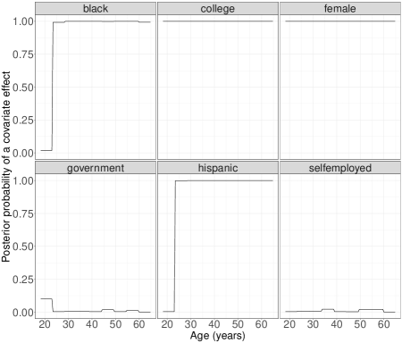
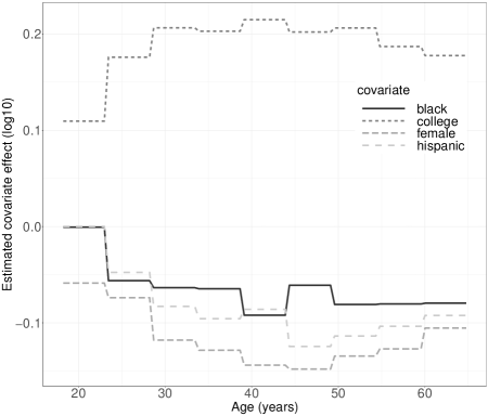
Figure 3. Salary Data, discussed in Section 5.3. Left: posterior probability of a salary gap associated with race, gender and college education versus age, adjusted by occupation and worker class. Right: corresponding estimated effect (log-10 scale)

We used a dataset obtained from the 2019 Current Population Survey (Flood et al., 2020) to investigate the presence of a salary gap associated with potentially discriminatory factors, such as race (binary indicators for black race and Hispanic origin) and gender. The goal was to assess whether said gaps exist at all ages, and specifically for younger individuals who recently entered the workforce. The dataset includes $n=36,308$ single-race individuals aged 18-65 who were employed full-time (working 35-40 hours per week) and not serving in the military. The response variable is the log-10 annual work income. Besides assessing the effects of race and gender at various ages ($z$ coordinates), we included the possession of a university degree as a benchmark that is expected to have a positive effect across all ages. We also examined the effects of being government-employed and self-employed. We also included the occupational sector as an adjustment covariate. It is important to note that the inclusion of the occupational sector is predetermined and no testing is performed. The data contain information on 24 occupational sectors, such as architect/engineer, computer/maths, construction, farming, food, maintenance, etc.

We performed a multi-resolution analysis using two different resolutions, defining 10 and 20 local testing regions, respectively. These resolutions roughly corresponded to 5-year and 2.5-year bins, allowing us to examine the data at different age intervals. Figure 3 summarizes the results. The existence of gender and college education effect had a posterior probability near 1 at any age (left panel). However, these gaps were estimated to be smaller for younger individuals, aged $\leq 30$ (right panel). Specifically, college education was associated with higher salaries, while the female gender was associated with lower salaries at any age. Interestingly, we did not find evidence of salary gaps associated with black or Hispanic origins among individuals who had recently joined the workforce (aged 18-23). However, strong evidence was found for such gaps at all other ages. We must emphasize that the lack of evidence against a (local) null hypothesis does not prove its truth, as there may be limited power to detect such differences. However, given the large sample size, it appears that if there were truly a salary gap for individuals aged 18-23, it should not be very large. Finally, we also did not find evidence of salary gaps associated with being self- or government-employed. We remark that these findings should be interpreted conditional on the assumption that two individuals are equal in terms of their occupational sector, college education, and other covariates. Our analysis is not designed to detect discrimination that may hinder individuals from obtaining a certain education or occupation.

5.4. Local brain activity over time

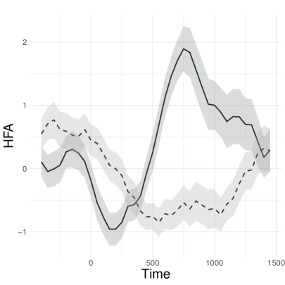
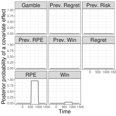
Figure 4. ECoG data. Left: mean high-frequency activity signal averaged across trials where the gamble was won (solid line) or lost (dashed line), and point-wise 80% confidence intervals. Right: posterior probability of local covariate effects on brain activity

We consider a dataset from Saez et al. (2018) measuring brain activity over time using multi-electrode electrocorticography. During the experiment, the patients played a game where they chose between a certain prize and a risky gamble, which had varying probabilities of higher winnings. The goal was to assess whether certain game-level covariates were associated with brain activation and, if so, at what specific times. We consider three covariates related to game outcomes: 1) whether the gamble resulted in a win or loss, 2) the reward prediction error (RPE) representing the difference between the obtained reward and the expected value of the gamble, and 3) the additional money that would have been won for the non-chosen option (regret). There was also a dummy covariate indicating whether participants chose to gamble or not and covariates about previous rounds (e.g. losing in the immediately preceding round).

Prior to time $z=0$ participants placed their bets. At exactly time $0$, the game’s outcome (money gained) was revealed to the participants. The researchers recorded the brain activity before and after the outcome revelation. Figure 4 (left) shows the mean high-frequency activity (HFA) signal for an illustrative electrode averaged across 179 trials played by a single patient, split according to whether the game was won (top) or lost (bottom). See Saez et al. (2018) for further experimental and data pre-processing details.

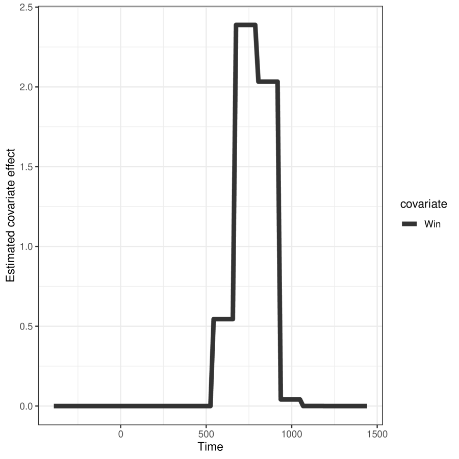
(a) Estimated effect of a Win/Loss over time

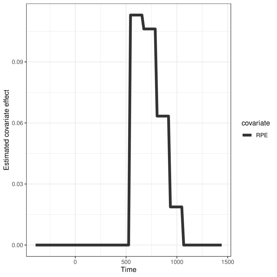
(b) Estimated effect of the reward prediction error (RPE) over time

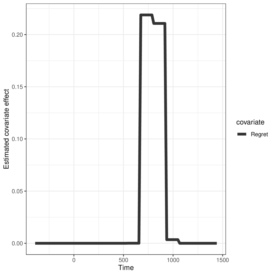
(c) Estimated effect of Regret over time

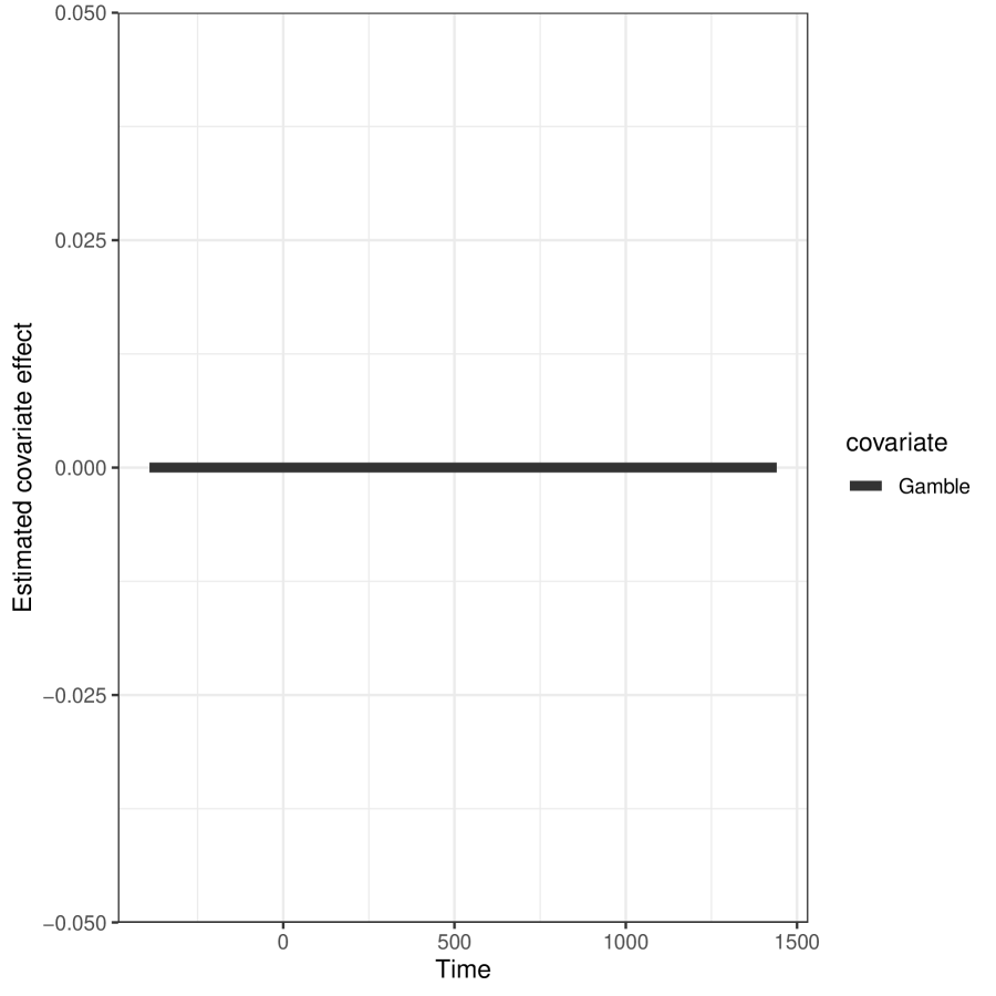
(d) Estimated effect of Gamble over time

Figure 8. Estimated time-varying effects of the three outcome-related covariates (Win, RPE, Regret) and the choice-related covariate Gamble in single-variate analyses for the application of Section 5.4.

Initially, we examined the local effect of each covariate separately. In this analysis, we focused on a time interval that extended from 450 ms before to 1500 ms after the outcome revelation, with knots placed at every 50-ms interval. This resolution should be sufficient to capture changes in brain activity typically observed in this type of experiment; for example, Saez et al. (2018) consider 50ms increments in a rolling window approach. We found a significant increase in HFA activity associated with game wins, higher reward prediction error, and regret. Specifically, the posterior probability of an effect for game wins was 0.9797 within the time range of $z\in(500,1000)$. Similar high probabilities were observed for regret (0.7566) and reward prediction error (0.999). Additionally, these effects displayed temporal variability, gradually decreasing over time, see Figure 8.

Subsequently, we conducted a multivariable analysis that included all eight mentioned covariates. This analysis revealed collinearity among the outcome-related covariates, leading to RPE being the only variable with a significant effect on HFA activity. Specifically, the posterior probability of an effect for RPE on HFA was approximately 0.949 within the time range of $z\in(500,1000)$. See Figure 4 (right).

Overall, our findings support that HFA activity is associated to outcome-related processes, such as gamble win or loss, RPE and regret, rather than choice-related processes like gamble choice. Further, that neural activity may be more highly associated with RPE than with wins. Therefore, our method helped disentangle highly correlated covariates and identify which ones can best explain variation in neural activity.

6. Discussion

Our framework is grounded in a semi-parametric model that assumes additive local covariate effects. We believe that this approach can provide more accurate inference compared to non-parametric methods in scenarios with moderate sample sizes or many covariates, while facilitating interpretation and computational efficiency. In all varying coefficient models such as ours, the evaluation of interactions between $z$ and $x$ is achieved by assessing changes in the coefficient values. Our approach tests the effect of a covariate in $x$, averaged across the values of other covariates in $x$. Although not done in our examples, to account for higher-order interactions within elements in $x$, one can augment the vector of covariates.

Our work focuses on testing multiple scientific hypotheses, rather than merely estimating the effects of covariates on the outcome. An alternative that a practitioner might consider is the use of credible intervals for covariate selection. However, this approach has several drawbacks. First, the pathological false positive inflation described here applies equally to confidence/credible intervals, unless one uses a construction ensuring the presence of zeroes in the asymptotic parameter values, e.g. the orthogonal cut basis presented here. Second, as pointed out by Berger and Delampady (1987), within a Bayesian framework this does not constitute an efficient testing procedure for a precise null hypothesis. Additionally, it fails to account for multiplicity, especially with dependent hypotheses: even with a small number of predictors, we may expect an increased proportion of falsely rejected null hypotheses. Finally, with a large number of covariates, a credible interval approach becomes highly inefficient, even in basic linear regression scenarios, compared to the exclusion of inactive covariates. Our formulation enables the use of standard algorithms for model search and posterior inference. These algorithms were effective in our examples, but computations become costlier when one considers many covariates, local testing regions or different resolutions. When many covariate effects are zero (sparse truth) the posterior distribution concentrates on small models, which eases computation, but for non-sparse truths it would be interesting to develop tailored computational algorithms. It would also be interesting to explore more refined covariance models beyond the simple parametric choices (e.g., auto-regressive and moving averages) considered in our examples. Such dependence models would be particularly relevant for settings with multivariate coordinates ($z$). However, the challenge lies in proposing statistically and computationally efficient methods despite the larger number of parameters involved.

Beyond our specific framework, we hope to shed light on subtle issues arising in local variable selection under misspecification, and help others put forward alternative solutions.

Supplementary material

The sections below contain all proofs, Lemma S1, and additional data analysis results. Additionally, folder 2023_Rossell_Kseung_Guindani_Saez_localvarsel contains data and R scripts to reproduce our results, available at https://github.com/davidrusi/paper_examples.

7. Proof of Lemma 1

To ease notation let $\mu=(\mu_{1}^{T},\ldots,\mu_{|\mathcal{R}|}^{T})^{T}$ where $\mu_{b}=E_{F}(y_{b}\mid X,Z)$. We obtain

$$\begin{pmatrix}\eta_{0}^{*}\\ \eta_{1}^{*}\end{pmatrix}=(W^{T}W)^{-1}W^{T}\mu=\begin{pmatrix}(W_{0}^{T}W_{0})^{-1}&0\\ 0&(W_{1}^{T}W_{1})^{-1}\end{pmatrix}\begin{pmatrix}W_{0}^{T}\\ W_{1}^{T}\end{pmatrix}\mu=\begin{pmatrix}(W_{0}^{T}W_{0})^{-1}W_{0}^{T}\\ (W_{1}^{T}W_{1})^{-1}W_{1}^{T}\end{pmatrix}\mu,$$

since $W_{1}^{T}W_{0}=0$. Now, note that (7) implies that $W_{1}^{T}W_{1}$ is block-diagonal, i.e.

$$W_{1}^{T}W_{1}=\begin{pmatrix}W_{11}^{T}W_{11}&0&\ldots&0\\ 0&W_{12}^{T}W_{12}&\ldots&0\\ \ldots&&&\ldots\\ 0&\ldots&&W_{1|\mathcal{R}|}^{T}W_{1|\mathcal{R}|}\end{pmatrix},$$

and hence

$$\begin{pmatrix}\eta_{11}^{*}\\ \ldots\\ \eta_{1|\mathcal{R}|}^{*}\end{pmatrix}=(W_{1}^{T}W_{1})^{-1}W_{1}^{T}\mu=$$

$$\begin{pmatrix}(W_{11}^{T}W_{11})^{-1}&0&\ldots&0\\ 0&(W_{12}^{T}W_{12})^{-1}&\ldots&0\\ \ldots&&&\ldots\\ 0&\ldots&&(W_{1|\mathcal{R}|}^{T}W_{1|\mathcal{R}|})^{-1}\end{pmatrix}\begin{pmatrix}W_{11}^{T}&0&\ldots&0\\ 0&W_{12}^{T}&\ldots&0\\ \ldots&&&\\ 0&0&\ldots&W_{1|\mathcal{R}|}^{T}\end{pmatrix}\begin{pmatrix}\mu_{1}\\ \mu_{2}\\ \ldots\\ \mu_{|\mathcal{R}|}\end{pmatrix}$$

and hence $\eta_{1b}^{*}=(W_{1b}^{T}W_{1b})^{-1}W_{1b}^{T}\mu_{b}$, as we wished to prove.

8. Orthogonal cut basis with multiple covariates

Recall that our assumed model is

$$y\mid Z,X\sim N(W_{0}\eta_{0}+W_{1}\eta_{1},\Sigma),$$

where $\Sigma$ is as in (4) and $(W_{0},W_{1})$ is an orthogonal cut matrix as in (7). Above $W_{1b}$ is obtained by multiplying a local cut basis by each covariate. Specifically,

$$W_{1b}=\begin{pmatrix}C_{b}\odot X_{b1},&\ldots,&C_{b}\odot X_{bp}\end{pmatrix},$$

where $C_{b}$ is the cut basis of region $b$, $X_{bj}$ is the column vector comprising the values of covariate $j$ for observations in region $b$, and $C_{b}\odot X_{bj}$ denotes the column-wise product obtained by multiplying each column in $C_{b}$ by $X_{bj}$, in an entry-wise fashion.

Let $\eta_{1j}=(\eta_{1j1}^{T},\ldots,\eta_{1j|\mathcal{R}|}^{T})^{T}$ where $\eta_{1jb}\in\mathbb{R}^{p}$ is the coefficient for the effect of covariate $j$ in region $b$. Then the model-based local null hypothesis for covariate $j$ in region $R_{b}$ is

(18) $$\beta_{1j}(z)=0\mbox{ for all }z\in R_{b}\Longleftrightarrow\eta_{1jb}=0.$$

Since $W_{1}$ is an orthogonal cut basis, Lemmas 1 and 2 directly apply to (18). In fact, the statement and proof of Lemma 2 are given explicitly multiple covariate case. This means that if $E_{F}(y_{b}\mid X,Z)$ is linearly independent of covariate $j$ given the other covariates, then the asymptotic covariate effect in region $b$ is $\eta_{1jb}^{*}=0$ (for dependent data, $\tilde{\eta}_{1jb}^{*}=0$).

9. Lemma 2

Lemma 2 extends Lemma 1 to dependent data settings where for each individual one observes data on a grid (e.g. longitudinal or functional data). Specifically, let $y_{i}$ be observation $i=1,\ldots,n$, $m_{i}=1,\ldots,M$ denote the individual and $M$ the number of individuals, and $x_{i}=x_{m_{i}}$ be the covariates for individual $m_{i}$ (in particular, for group comparisons $x_{m_{i}}$ is a vector coding for group membership). Suppose that for each individual we have the same number of measurements $n/M$.

We first recall the notation and setup. Recall that the assumed model is

$$y\mid Z,X\sim N\left(W_{0}\eta_{0}+W_{1}\eta_{1},\Sigma\right),$$

where $(W_{0},W_{1})$ are orthogonal cut basis as defined in Section 1.2. Recall that these can be written as

(19) $$W_{0}=\begin{pmatrix}W_{01}\\ W_{02}\\ \ldots\\ W_{0|\mathcal{R}|}\end{pmatrix};\hskip 14.22636ptW_{1}=\begin{pmatrix}W_{11}&0&\ldots&0\\ 0&W_{12}&\ldots&0\\ \ldots&&&\\ 0&0&\ldots&W_{1|\mathcal{R}|},\end{pmatrix}.$$

where $W_{1b}$ is the basis evaluated at region $b=1,\ldots,|\mathcal{R}|$ interacted with the covariate effects. Specifically,

$$W_{1b}=\begin{pmatrix}C_{b}\odot X_{b1},&\ldots,&C_{b}\odot X_{bp}\end{pmatrix},$$

where $C_{b}$ is the cut basis of region $b$, $X_{bj}$ the column vector with the values of covariate $j$ for observations in region $b$, and $C_{b}\odot X_{bj}$ the column-wise product multiplying each column in $C_{b}$ by $X_{bj}$, in an entry-wise fashion.

Finally, recall also that $\Sigma$ is assumed to have a block-diagonal structure across regions, i.e.

$$\Sigma=\begin{pmatrix}\Sigma_{1}&0&\ldots&0\\ 0&\Sigma_{2}&\ldots&0\\ \ldots&&&\\ 0&0&\ldots&\Sigma_{|\mathcal{R}|}\end{pmatrix}.$$

Denote by $\widetilde{\eta}^{*}=(\widetilde{\eta}_{0}^{*},\widetilde{\eta}_{1}^{*})$ the Kullback-Leibler optimal parameter value under the data-generating truth $F$. That is,

$$\widetilde{\eta}^{*} =\arg\min_{\eta}E_{F}\left[(y-W\eta)^{T}\Sigma^{-1}(y-W\eta)\mid Z,X\right]=(W^{T}\Sigma^{-1}W)^{-1}W^{T}\Sigma^{-1}E_{F}(y\mid Z,X)$$

Lemma 2.

Let $W=(W_{0},W_{1})$ where $W_{1}$ is orthogonal cut basis as in (7) satisfying $W_{0}^{T}W_{1}=0$. Suppose that for each individual one has the same number of measurements $n/M$, and that covariate values add to zero across individuals, i.e. $\sum_{m=1}^{M}x_{s_{i}}=0$.

Let $\widetilde{\eta}_{1}^{*}=(\widetilde{\eta}_{11},\ldots,\widetilde{\eta}_{1|\mathcal{R}|}^{*})$ where $\widetilde{\eta}_{1b}$ are the parameters associated to $W_{1b}$ (i.e. to region $b$). Then,

$$\widetilde{\eta}_{1b}^{*}=(W_{1b}^{T}\Sigma_{b}^{-1}W_{1b})^{-1}W_{1b}^{T}\Sigma_{b}^{-1}E_{F}(y_{b}\mid X,Z).$$

Proof.

Let $\widetilde{W}=\Sigma^{-1/2}W$ and $\tilde{y}=\Sigma^{-1/2}y$, the optimal solution can then be written as

$$\widetilde{\eta}^{*} =(\widetilde{W}^{T}\widetilde{W})^{-1}\widetilde{W}^{T}E_{F}(\widetilde{y}\mid Z,X).$$

The proof strategy is to show that the conditions of Lemma 1 hold for $\widetilde{W}=(\widetilde{W}_{0},\widetilde{W}_{1})=(\Sigma^{-1/2}W_{0},\Sigma^{-1}W_{1})$, which then immediately gives that

$$\widetilde{\eta}_{1b}^{*}=(\widetilde{W}_{1b}^{T}\widetilde{W}_{1b})^{-1}\widetilde{W}_{1b}^{T}E_{F}(\tilde{y}_{b}\mid X,Z)=(W_{1b}^{T}\Sigma_{b}^{-1}W_{1b})^{-1}W_{1b}^{T}\Sigma_{b}^{-1}E_{F}(y_{b}\mid X,Z),$$

where we used that $\tilde{y}_{b}=\Sigma^{-1/2}y_{b}$, proving Lemma 2.

The first condition in Lemma 1 is that $\widetilde{W}_{1}$ is a cut matrix. To see that this holds, note that $\widetilde{W}_{1}=\Sigma^{-1/2}W_{1}=$

$$\begin{pmatrix}\Sigma_{1}&0&\ldots&0\\ 0&\Sigma_{2}&\ldots&0\\ \ldots&&&\\ 0&0&\ldots&\Sigma_{|\mathcal{R}|}\end{pmatrix}\begin{pmatrix}W_{11}&0&\ldots&0\\ 0&W_{12}&\ldots&0\\ \ldots&&&\\ 0&0&\ldots&W_{1|\mathcal{R}|}\end{pmatrix}=\begin{pmatrix}\widetilde{W}_{11}&0&\ldots&0\\ 0&\widetilde{W}_{12}&\ldots&0\\ \ldots&&&\\ 0&0&\ldots&\widetilde{W}_{1|\mathcal{R}|},\end{pmatrix}$$

where $\widetilde{W}_{1b}=\Sigma_{b}^{-1}W_{1b}$. This proves that $\widetilde{W}_{1}$ has the same structure as $W_{1}$ in 19, i.e. $\widetilde{W}_{1}$ is a cut basis.

The second condition in Lemma 1 is that $\widetilde{W}_{1}$ is an orthogonal basis to $\widetilde{W}_{0}$, i.e. $\widetilde{W}_{0}^{T}\widetilde{W}_{1}=0$. To show that this condition holds, first note that

$$\widetilde{W}_{0}^{T}\widetilde{W}_{1}=\widetilde{W}_{0}^{T}\begin{pmatrix}\widetilde{W}_{11}&0&\ldots&0\\ 0&\widetilde{W}_{12}&\ldots&0\\ \ldots&&&\\ 0&0&\ldots&\widetilde{W}_{1|\mathcal{R}|},\end{pmatrix}=\begin{pmatrix}\widetilde{W}_{01}^{T}\widetilde{W}_{11}\\ \widetilde{W}_{02}^{T}\widetilde{W}_{12}\\ \ldots\\ \widetilde{W}_{0|\mathcal{R}|}^{T}\widetilde{W}_{1|\mathcal{R}|},\end{pmatrix},$$

where $\widetilde{W}_{0b}$ are the rows from $\widetilde{W}_{0}$ corresponding to region $b$. Hence, it suffices to show that $\widetilde{W}_{0b}^{T}\widetilde{W}_{1b}=0$ for all $b$. To see this, note that $\widetilde{W}_{0b}^{T}\widetilde{W}_{1b}$ can be computed by summing across individuals $s=1,\ldots,m$. That is,

$$\widetilde{W}_{0b}^{T}\widetilde{W}_{1b}=\sum_{m=1}^{M}\widetilde{W}_{0bm}^{T}\widetilde{W}_{1bm}.$$

Since all individuals are observed on the same grid we have that $W_{0bm}$ is constant across $m$, and similarly $\Sigma_{bm}$ is assumed constant across individuals, hence we may write $\widetilde{W}_{0bm}=\Sigma_{bm}^{-1/2}W_{0bm}=T_{0b}$, where $T_{0b}$ does not depend on the individual $m$. Similarly,

$$\widetilde{W}_{1bm}=\Sigma_{bm}^{-1/2}W_{1bm}=\Sigma_{bm}^{-1/2}\begin{pmatrix}C_{bm}\odot X_{bm1},&\ldots,&C_{bm}\odot X_{bmp}\end{pmatrix}=T_{1b}x_{m}$$

where $X_{bmj}$ is the column vector with the value of covariate $j$ for individual $m$, that is constant across observations in region $b$ and equal to $x_{mj}$, and $T_{1b}=\Sigma_{bm}^{-1}C_{bm}$ does not depend on $m$ (since all individuals are observed on the same grid, $C_{bm}$ is constant across individuals indexed by $m$). Recall that $x_{m}=(x_{m1},\ldots,x_{mp})$ denotes the covariates for individual $m$. We therefore obtain that

$$\widetilde{W}_{0b}^{T}\widetilde{W}_{1b}=\sum_{m=1}^{M}\widetilde{W}_{0bm}^{T}\widetilde{W}_{1bm}=T_{0b}^{T}T_{1b}\sum_{m=1}^{M}x_{m}=0,$$

since $\sum_{m=1}^{M}x_{m}=0$ (the covariates have zero sample mean) by assumption, completing the proof.

∎

10. Bayes factor derivation

The Bayes factor comparing a model $\gamma$ with the optimal $\gamma^{*}$ is

(20) $$\begin{split}B_{\gamma\gamma^{*}}&=\frac{\left|gV_{\gamma^{*}}W_{\gamma^{*}}^{T}\Sigma^{-1}W_{\gamma^{*}}+I\right|^{\frac{1}{2}}}{\left|gV_{\gamma}W_{\gamma}^{T}\Sigma^{-1}W_{\gamma}+I\right|^{\frac{1}{2}}}\\ &\times\exp\left\{\frac{1}{2}\left[\hat{\eta}_{\gamma}^{T}(W_{\gamma}^{T}\Sigma^{-1}W_{\gamma}+(gV_{\gamma})^{-1})\hat{\eta}_{\gamma}-\hat{\eta}_{\gamma^{*}}^{T}(W_{\gamma^{*}}^{T}\Sigma^{-1}W_{\gamma^{*}}+(gV_{\gamma^{*}})^{-1})\hat{\eta}_{\gamma^{*}}\right]\right\},\end{split}$$

where $\hat{\eta}_{\gamma}=E(\eta_{\gamma}\mid y,\gamma)=(W_{\gamma}^{T}\Sigma^{-1}W_{\gamma}+(gV_{\gamma})^{-1})^{-1}W_{\gamma}^{T}\Sigma^{-1}y$.

We derive Expression (20). Recall that the assumed model is

$$y\mid\gamma \sim N(W_{\gamma}\eta_{\gamma},\Sigma)$$

$$\beta_{\gamma} \sim N(0,gV_{\gamma}),$$

where $\Sigma$ is an $n\times n$ and $V_{\gamma}$ a $|\gamma|_{0}\times|\gamma|_{0}$ positive-definite matrix, and $g\in\mathbb{R}^{+}$.

The integrated likelihood under model $\gamma$ is hence

$$p(y\mid\gamma)=\int\frac{1}{(2\pi)^{\frac{n}{2}}|\Sigma|^{\frac{1}{2}}|gV_{\gamma}|^{\frac{1}{2}}}e^{-\frac{1}{2}(y-W_{\gamma}\eta_{\gamma})^{T}\Sigma^{-1}(y-W_{\gamma}\eta_{\gamma})}\frac{1}{(2\pi)^{\frac{|\gamma|_{0}}{2}}}e^{-\frac{1}{2}\eta_{\gamma}^{T}(gV_{\gamma})^{-1}\eta_{\gamma}}d\eta_{\gamma}$$

$$=\frac{e^{-\frac{1}{2}y^{T}\Sigma^{-1}y}}{(2\pi)^{\frac{n}{2}}|\Sigma|^{\frac{1}{2}}|gV_{\gamma}|^{\frac{1}{2}}}\int\frac{1}{(2\pi)^{\frac{|\gamma|_{0}}{2}}}e^{-\frac{1}{2}\left[\eta_{\gamma}^{T}(W_{\gamma}^{T}\Sigma^{-1}W_{\gamma}+(gV_{\gamma})^{-1})\eta_{\gamma}-2y^{T}\Sigma^{-1}W_{\gamma}\eta_{\gamma}\right]}d\eta_{\gamma}.$$

Denoting by $V_{post}=(W_{\gamma}^{T}\Sigma^{-1}W_{\gamma}+(gV_{\gamma})^{-1})^{-1}$ and $\hat{\eta}_{\gamma}=(W_{\gamma}^{T}\Sigma^{-1}W_{\gamma}+(gV_{\gamma})^{-1})^{-1}W_{\gamma}^{T}\Sigma^{-1}y$, we obtain

$$p(y\mid\gamma)=\frac{e^{-\frac{1}{2}y^{T}\Sigma^{-1}y}e^{\frac{1}{2}\hat{\eta}_{\gamma}^{T}V_{post}^{-1}\hat{\eta}_{\gamma}}}{(2\pi)^{\frac{n}{2}}|\Sigma|^{\frac{1}{2}}|gV_{\gamma}|^{\frac{1}{2}}}\int\frac{1}{(2\pi)^{\frac{|\gamma|_{0}}{2}}}e^{-\frac{1}{2}\left[\eta_{\gamma}^{T}V_{post}^{-1}\eta_{\gamma}-2y^{T}\Sigma^{-1}W_{\gamma}V_{post}V_{post}^{-1}\eta_{\gamma}+\hat{\eta}_{\gamma}^{T}V_{post}^{-1}\hat{\eta}_{\gamma}\right]}d\eta_{\gamma}=$$

$$\frac{e^{-\frac{1}{2}y^{T}\Sigma^{-1}y}e^{\frac{1}{2}\hat{\eta}_{\gamma}^{T}V_{post}^{-1}\hat{\eta}_{\gamma}}}{(2\pi)^{\frac{n}{2}}|\Sigma|^{\frac{1}{2}}|gV_{\gamma}|^{\frac{1}{2}}}\int\frac{1}{(2\pi)^{\frac{|\gamma|_{0}}{2}}}e^{-\frac{1}{2}(\eta_{\gamma}-\hat{\eta}_{\gamma})^{T}V_{post}^{-1}(\eta_{\gamma}-\hat{\eta}_{\gamma})}d\eta_{\gamma}=\frac{e^{-\frac{1}{2}y^{T}\Sigma^{-1}y}e^{\frac{1}{2}\hat{\eta}_{\gamma}^{T}V_{post}^{-1}\hat{\eta}_{\gamma}}|V_{post}|^{\frac{1}{2}}}{(2\pi)^{\frac{n}{2}}|\Sigma|^{\frac{1}{2}}|gV_{\gamma}|^{\frac{1}{2}}}.$$

Hence the Bayes factor is $B_{\gamma\gamma^{*}}=p(y\mid\gamma)/p(y\mid\gamma^{*})=$

$$e^{\frac{1}{2}[\hat{\eta}_{\gamma}^{T}(W_{\gamma}^{T}\Sigma^{-1}W_{\gamma}+(gV_{\gamma})^{-1})\hat{\eta}_{\gamma}-\hat{\eta}_{\gamma^{*}}^{T}(W_{\gamma^{*}}^{T}\Sigma^{-1}W_{\gamma^{*}}+(gV_{\gamma^{*}})^{-1})\hat{\eta}_{\gamma^{*}}]}\frac{|(W_{\gamma^{*}}^{T}\Sigma^{-1}W_{\gamma^{*}}+(gV_{\gamma^{*}})^{-1})gV_{\gamma^{*}}|^{\frac{1}{2}}}{|(W_{\gamma}^{T}\Sigma^{-1}W_{\gamma}+(gV_{\gamma})^{-1})gV_{\gamma}|^{\frac{1}{2}}},$$

as we wished to prove.

11. Discussion of the technical conditions of Theorem 1

Assumption (A1) implies that, although the number of parameters $q$ may be larger than $n$, we restrict our attention to full-rank models. This implies that the model size $|\gamma|_{0}\leq n$, a common practice in model selection. Assumption (A2) is a mild and can be relaxed, but simplifies our exposition. In our default setting, we assume $V_{\gamma}=I$. Thus (A2) is satisfied when the empirical covariance $W_{\gamma}^{T}\Sigma^{-1}W_{\gamma}/n$ converges to a fixed positive definite covariance. The assumption is also satisfied by Zellner’s prior, where $V_{\gamma}^{-1}=W_{\gamma}^{T}\Sigma^{-1}W_{\gamma}/n$, so that $\underline{l}_{\gamma}=\bar{l}_{\gamma}$. Assumption (A3) holds in the homoskedastic independent errors setting where $\Sigma=\sigma^{2}I$. For dependent data, (A3) is a mild condition that may be relaxed to accommodate cases where $\tau$ is not bounded as $n$ grows, see the proof of Theorem 1. Assumption (A4) is minimal and ensures that the prior dispersion $g$ does not vanish too fast with $n$ (it is satisfied by our default $g=1$ and by the discussed alternatives where $g$ may grow with $n$). In Assumption (A5) the parameter $\lambda_{\gamma}$ can be interpreted as a non-centrality parameter that measures the sum of squares explained by model $\gamma^{*}$ but not by model $\gamma$. Assumption (A5) is minimal: otherwise, Bayes factors are not consistent even in finite-dimensional settings with fixed $|\gamma|_{0}$. See also the discussion of Assumption (B6) in Section 4.2 on the relationship between $\lambda_{\gamma}$ and common beta-min and restricted eigenvalue conditions.

12. Auxiliary results for Theorem 1

We recall auxiliary results that are helpful in the proofs of our main results. Lemmas 3-7 are obtained from Sections S6 and S9 in Rossell et al. (2021). For brevity we do not reproduce their proofs, please see Sections S6 and S9 in Rossell et al. (2021). However, we do prove Lemma 7 here since, although the result in Rossell et al. (2021) is correct, the proof offered there contains an error.

Lemma 8 is a new result that we prove here bounding tail probabilities for certain differences between quadratic forms of sub-Gaussian vectors.

Lemma 3 is a well-known result. It expresses the difference between the explained sum of squares by two nested models $\gamma^{\prime}\subset\gamma$ in terms of the regression parameters obtained under the larger model, after suitably orthogonalizing its design matrix.

Definition 1 and Lemmas 4-5 give the definition and two basic properties of sub-Gaussian random vectors: closed-ness under linear combinations and hat certain quadratic forms of $n$-dimensional sub-Gaussian vectors can be re-expressed as a quadratic form of $d$-dimensional sub-Gaussian vectors. Lemmas 6-7 give bounds for right and left sub-Gaussian tail probabilities.

Lemma 3.

Let $y\in\mathbb{R}^{n}$ and $W_{\gamma}=(W_{\gamma^{\prime}},W_{\gamma\setminus\gamma^{\prime}})$ be an $n$ times $|\gamma|_{0}$ matrix. Let $\hat{\eta}_{\gamma}=(W_{\gamma}^{T}W_{\gamma})^{-1}W_{\gamma}^{T}y$ and $\hat{\eta}_{\gamma^{\prime}}=(W_{\gamma^{\prime}}^{T}W_{\gamma^{\prime}})^{-1}W_{\gamma^{\prime}}^{T}y$ the least-squares estimates associated to $\gamma$ and $\gamma^{\prime}$, respectively. Then

$$\hat{\eta}_{\gamma}^{T}W_{\gamma}^{T}W_{\gamma}\hat{\eta}_{\gamma}-\hat{\eta}_{\gamma^{\prime}}^{T}W_{\gamma^{\prime}}^{T}W_{\gamma^{\prime}}\hat{\eta}_{\gamma^{\prime}}=\tilde{\eta}_{\gamma\setminus\gamma^{\prime}}^{T}\tilde{W}_{\gamma\setminus\gamma^{\prime}}^{T}\tilde{W}_{\gamma\setminus\gamma^{\prime}}\tilde{\eta}_{\gamma\setminus\gamma^{\prime}}=y^{T}\tilde{W}_{\gamma\setminus\gamma^{\prime}}(\tilde{W}_{\gamma\setminus\gamma^{\prime}}^{T}\tilde{W}_{\gamma\setminus\gamma^{\prime}})^{-1}\tilde{W}_{\gamma\setminus\gamma^{\prime}}^{T}y$$

where $\tilde{\eta}_{\gamma\setminus\gamma^{\prime}}=(\tilde{W}_{\gamma\setminus\gamma^{\prime}}^{T}\tilde{W}_{\gamma\setminus\gamma^{\prime}})^{-1}\tilde{W}_{\gamma\setminus\gamma^{\prime}}^{T}y$ and $\tilde{W}_{\gamma\setminus\gamma^{\prime}}=W_{\gamma\setminus\gamma^{\prime}}-W_{\gamma^{\prime}}(W_{\gamma^{\prime}}^{T}W_{\gamma^{\prime}})^{-1}W_{\gamma^{\prime}}^{T}W_{\gamma\setminus\gamma^{\prime}}$.

Definition 1.

A $d$-dimensional random vector $s=(s_{1},\ldots,s_{d})$ follows a sub-Gaussian distribution with parameters $\mu\in\mathbb{R}^{d}$ and $\sigma^{2}>0$, which we denote by $s\sim\mbox{SG}(\mu,\sigma^{2})$ if and only if

$$E\left[\exp\{\alpha^{T}(s-\mu)\}\right]\leq\exp\{\alpha^{T}\alpha\sigma^{2}/2\}$$

for all $\alpha\in\mathbb{R}^{d}$.

Lemma 4.

Let $s\sim\mbox{SG}(\mu,\sigma^{2})$ be a sub-Gaussian $d$-dimensional random vector, and $A$ be a $q\times d$ matrix. Then $As\sim\mbox{SG}(A\mu,\lambda\sigma^{2})$, where $\lambda$ is the largest eigenvalue of $A^{T}A$, or equivalently the largest eigenvalue of $AA^{T}$.

Lemma 5.

Let $y\sim\mbox{SG}(\mu,\sigma^{2})$ be an $n$-dimensional sub-Gaussian random vector. Let $W=(y-a)^{T}X(X^{T}X)^{-1}X^{T}(y-a)$, where $X$ is an $n\times d$ matrix such that $X^{T}X$ is invertible. Then $W=s^{T}s$, where $s\sim\mbox{SG}((X^{T}X)^{-1/2}X^{T}(\mu-a),\sigma^{2})$ is $d$-dimensional.

Lemma 6.

Central sub-Gaussian quadratic forms. Right-tail probabilities Let $s=(s_{1},\ldots,s_{d})\sim\mbox{SG}(0,\sigma^{2})$. Then

1. For any $t>0$,

   $$P\left(\frac{s^{T}s}{\sigma^{2}}>dt[1+\sqrt{2/t}+1/t]\right)\leq\exp\left\{-\frac{dt}{2}\right\}.$$

2. For any $q>0$ and any $k_{0}$ such that $k_{0}\geq\frac{(1+k_{0})}{q}+\sqrt{\frac{2(1+k_{0})}{q}}$,

   $$P\left(\frac{s^{T}s}{\sigma^{2}}>dq\right)\leq\exp\left\{-\frac{dq}{2(1+k_{0})}\right\}$$

3. For any $q\geq 2(1+\sqrt{2})^{2}$,

   $$P\left(\frac{s^{T}s}{\sigma^{2}}>dq\right)\leq\exp\left\{-\frac{dq}{2(1+k_{0})}\right\}$$

   where $k_{0}\geq\sqrt{2}(1+\sqrt{2})/\sqrt{q}$.

Lemma 7.

Non-central sub-Gaussian quadratic forms. Left-tail probabilities Let $s=(s_{1},\ldots,s_{d})\sim\mbox{SG}(\mu,\sigma^{2})$ and $a\in(0,\mu^{T}\mu)$. Then

$$P(s^{T}s<a)\leq\exp\left\{-\frac{\mu^{T}\mu}{8\sigma^{2}}\left(1-\frac{a}{\mu^{T}\mu}\right)^{2}\right\}.$$

Proof.

of Lemma 7. For any $t>0$ and $a>0$, it holds that

$$P(s^{T}s<a)=P\left(e^{-ts^{T}s}>e^{-ta}\right)\leq e^{ta}E(e^{-ts^{T}s}),$$

where the right-hand side follows from Markov’s inequality. Since $s=z+\mu$ where $z\sim SG(0,\sigma^{2})$, we obtain

$$P(s^{T}s<a)\leq e^{ta}E(e^{-t[(z+\mu)^{T}(z+\mu)]})=e^{t(a-\mu^{T}\mu)}E\left(\frac{e^{-2t\mu^{T}z}}{e^{tz^{T}z}}\right)\leq e^{t(a-\mu^{T}\mu)}E\left(e^{-2t\mu^{T}z}\right),$$

where we used that $e^{-tz^{T}z}\leq 1$. Using the definition of sub-Gaussianity to bound the expectation on the right-hand side gives

$$P(s^{T}s<a)\leq e^{t(a-\mu^{T}\mu)+2t^{2}\mu^{T}\mu\sigma^{2}}.$$

The bound above holds for any $t>0$. The optimal $t$ is found by setting the first derivative to zero, which gives

$$t=\frac{\mu^{T}\mu-a}{4\mu^{T}\mu\sigma^{2}}.$$

Note that to have $t>0$, we need that $a<\mu^{T}\mu$, which holds by assumption. Plugging in the optimal $t$ into the upper-bound gives

$$P(s^{T}s<a) \leq\exp\left\{-\frac{(a-\mu^{T}\mu)^{2}}{4\mu^{T}\mu\sigma^{2}}+\frac{\mu^{T}\mu\sigma^{2}(\mu^{T}\mu-a)^{2}}{8(\mu^{T}\mu)^{2}\sigma^{4}}\right\}$$

$$=\exp\left\{-\frac{(\mu^{T}\mu-a)^{2}}{8\mu^{T}\mu\sigma^{2}}\right\}=\exp\left\{-\frac{\mu^{T}\mu}{8\sigma^{2}}\left(1-\frac{a}{\mu^{T}\mu}\right)^{2}\right\},$$

as we wished to prove. ∎

Lemma 8.

Tail probabilities for differences of sub-Gaussian quadratic forms Let $u_{1}\sim SG(0,\sigma^{2})$ be a $d_{1}$-dimensional sub-Gaussian vector and $u_{2}\sim SG(\mu,\sigma^{2})$ a $d_{2}$-dimensional sub-Gaussian vector, where $\sigma^{2}>0$ is finite and $\mu\in\mathbb{R}^{d_{2}}$.

1. Let $a>0$, then

   $$P\left(\frac{au_{1}^{T}u_{1}-u_{2}^{T}u_{2}}{\sigma^{2}}>t\right)\leq\exp\left\{-\frac{d_{1}q}{2(1+k_{0})}\right\}+\exp\left\{-\frac{\mu^{T}\mu}{8\sigma^{2}}\left(1-\frac{1}{\log\mu^{T}\mu}\right)\right\},$$

   for any $t$ such that

   $$q:=\frac{t}{ad_{1}}+\frac{\mu^{T}\mu}{ad_{1}\sigma^{2}\log\mu^{T}\mu}\geq 2(1+\sqrt{2})^{2}$$

   and $k_{0}=\sqrt{2}(1+\sqrt{2})/\sqrt{q}$.

   In particular, for $t=d\log h$ where $d,h>0$,

   $$P\left(\frac{u_{1}^{T}u_{1}-u_{2}^{T}u_{2}}{\sigma^{2}}>t\right)\leq h^{-\frac{d}{2a(1+k_{0})}}e^{-\frac{\mu^{T}\mu}{2a(1+k_{0})\sigma^{2}\log\mu^{T}\mu}}+\exp\left\{-\frac{\mu^{T}\mu}{8\sigma^{2}}\left(1-\frac{1}{\log\mu^{T}\mu}\right)\right\}.$$

2. Let $t\geq 2(1+\sqrt{2})^{2}ad_{1}$. Then

   $$P\left(\frac{au_{1}^{T}u_{1}-u_{2}^{T}u_{2}}{\sigma^{2}}>t\right)\leq\exp\left\{-\frac{t}{2(1+k_{0})a}\right\},$$

for any $k_{0}\geq\sqrt{2}(1+\sqrt{2})\sqrt{ad_{1}/t}$.

Proof.

of Lemma 8, Part (i). Let $\lambda=\mu^{T}\mu$. The union bound gives that, for any $t^{\prime}>0$,

$$P\left(\frac{au_{1}^{T}u_{1}-u_{2}^{T}u_{2}}{\sigma^{2}}>t\right)=P\left(\frac{au_{1}^{T}u_{1}-u_{2}^{T}u_{2}}{\sigma^{2}}>\frac{t}{2}+t^{\prime}-\left[t^{\prime}-\frac{t}{2}\right]\right)$$

(21) $$\leq P\left(\frac{u_{1}^{T}u_{1}}{\sigma^{2}}>\frac{t}{2}+t^{\prime}\right)+P\left(\frac{u_{2}^{T}u_{2}}{\sigma^{2}}<t^{\prime}-\frac{t}{2}\right).$$

In particular take $t^{\prime}=t/2+\lambda/[\sigma^{2}\log\lambda]$, so that $t^{\prime}-t/2=\lambda/[\sigma^{2}\log\lambda]$ and $t^{\prime}+t/2=t+\lambda/[\sigma^{2}\log\lambda]$. Then, using Lemma 7 we have that the second term in (21) is

(22) $$P\left(\frac{u_{2}^{T}u_{2}}{\sigma^{2}}<\frac{\lambda}{\sigma^{2}\log\lambda}\right)\leq\exp\left\{-\frac{\lambda}{8\sigma^{2}}\left(1-\frac{1}{\log\lambda}\right)\right\}.$$

The first term in (21) is

(23) $$P\left(\frac{u_{1}^{T}u_{1}}{\sigma^{2}}>\frac{t}{a}+\frac{\lambda}{a\sigma^{2}\log\lambda}\right)=P\left(\frac{u_{1}^{T}u_{1}}{\sigma^{2}}>d_{1}\left[\frac{t}{d_{1}a}+\frac{\lambda}{d_{1}a\sigma^{2}\log\lambda}\right]\right).$$

Since

(24) $$q=\frac{t}{d_{1}a}+\frac{\lambda}{d_{1}a\sigma^{2}\log\lambda}\geq 2(1+\sqrt{2})^{2},$$

by assumption, Lemma 6(iii) gives that (23) is

$$\leq\exp\left\{-\frac{d_{1}q}{2(1+k_{0})}\right\}.$$

Combining (23) and (22) gives

$$P\left(\frac{au_{1}^{T}u_{1}-u_{2}^{T}u_{2}}{\sigma^{2}}>t\right)\leq\exp\left\{-\frac{d_{1}q}{2(1+k_{0})}\right\}+\exp\left\{-\frac{\lambda}{8\sigma^{2}}\left(1-\frac{1}{\log\lambda}\right)\right\},$$

as we wished to prove. Finally, for the particular case where one plugs in $t=d\log h$ where $d,h>0$ satisfy the condition (24) above, gives

$$q=\frac{d\log h}{d_{1}a}+\frac{\lambda}{d_{1}a\sigma^{2}\log\lambda}$$

and hence

$$\exp\left\{-\frac{d_{1}q}{2(1+k_{0})}\right\}=\exp\left\{-\frac{1}{2a(1+k_{0})}\left[d\log h+\frac{\lambda}{\sigma^{2}\log\lambda}\right]\right\}=h^{-\frac{d}{2a(1+k_{0})}}e^{-\frac{\lambda}{2a(1+k_{0})\sigma^{2}\log\lambda}}.$$

∎

Proof.

of Lemma 8, Part (ii). Since $au_{1}^{T}u_{1}-u_{2}^{T}u_{2}\leq au_{1}^{T}u_{1}$, it follows that

$$P\left(\frac{au_{1}^{T}u_{1}-u_{2}^{T}u_{2}}{\sigma^{2}}>t\right)\leq P\left(\frac{au_{1}^{T}u_{1}}{\sigma^{2}}>t\right)=P\left(\frac{u_{1}^{T}u_{1}}{\sigma^{2}}>d_{1}\frac{t}{ad_{1}}\right).$$

Using Lemma 6(iii) gives that the right-hand side is

$$\leq\exp\left\{-\frac{t}{2(1+k_{0})a}\right\}$$

for any $t/(ad_{1})\geq 2(1+\sqrt{2})^{2}$ and $k_{0}\geq\sqrt{2}(1+\sqrt{2})\sqrt{ad_{1}/t}$, as we wished to prove. ∎

13. Proof of Theorem 1

Recall that the Bayes factor is

$$B_{\gamma\gamma^{*}} =\frac{\left|gV_{\gamma^{*}}W_{\gamma^{*}}^{T}\Sigma^{-1}W_{\gamma^{*}}+I\right|^{\frac{1}{2}}}{\left|gV_{\gamma}W_{\gamma}^{T}\Sigma^{-1}W_{\gamma}+I\right|^{\frac{1}{2}}}$$

(25) $$\times\exp\left\{\frac{1}{2}\left[\hat{\eta}_{\gamma}^{T}(W_{\gamma}^{T}\Sigma^{-1}W_{\gamma}+(gV_{\gamma})^{-1})\hat{\eta}_{\gamma}-\hat{\eta}_{\gamma^{*}}^{T}(W_{\gamma^{*}}^{T}\Sigma^{-1}W_{\gamma^{*}}+(gV_{\gamma^{*}})^{-1})\hat{\eta}_{\gamma^{*}}\right]\right\},$$

where $\hat{\eta}_{\gamma}=E(\eta_{\gamma}\mid y,\gamma)=(W_{\gamma}^{T}\Sigma^{-1}W_{\gamma}+(gV_{\gamma})^{-1})^{-1}W_{\gamma}^{T}\Sigma^{-1}y$.

The proof strategy is as follows. First we show that the first term in (25) is essentially given by $(gn)^{(|\gamma^{*}|_{0}-|\gamma|_{0})/2}$ (up to lower-order terms). To characterize the second term in (25) we note that the terms in the exponent are a Bayesian version of the sum of explained squares under model $\gamma$ minus that for $\gamma^{*}$, show that these are essentially equivalent to the least-squares counterparts. The latter sum-of-squares can be re-written as a quadratic form of sub-Gaussian vectors using Lemma 3, which can be bounded using the inequalities developed in Section 12.

Consider the first term in (25). Under Assumption (A2) the eigenvalues of $gV_{\gamma}W_{\gamma}^{T}\Sigma^{-1}W_{\gamma}+I$ lie in $(gn\underline{l}_{\gamma}+1,gn\bar{l}_{\gamma}+1)$, hence

$$\frac{(gn\underline{l}_{\gamma^{*}})^{\frac{|\gamma^{*}|_{0}}{2}}}{(gn\bar{l}_{\gamma}+1)^{\frac{|\gamma|_{0}}{2}}}\leq\frac{(gn\underline{l}_{\gamma^{*}}+1)^{\frac{|\gamma^{*}|_{0}}{2}}}{(gn\bar{l}_{\gamma}+1)^{\frac{|\gamma|_{0}}{2}}}\leq\frac{\left|gV_{\gamma^{*}}W_{\gamma^{*}}^{T}\Sigma^{-1}W_{\gamma^{*}}+I\right|^{\frac{1}{2}}}{\left|gV_{\gamma}W_{\gamma}^{T}\Sigma^{-1}W_{\gamma}+I\right|^{\frac{1}{2}}}\leq\frac{(gn\bar{l}_{\gamma^{*}}+1)^{\frac{|\gamma^{*}|_{0}}{2}}}{(gn\underline{l}_{\gamma}+1)^{\frac{|\gamma|_{0}}{2}}}\leq\frac{(gn\bar{l}_{\gamma^{*}}+1)^{\frac{|\gamma^{*}|_{0}}{2}}}{(gn\underline{l}_{\gamma})^{\frac{|\gamma|_{0}}{2}}}.$$

Using that $\lim_{n\rightarrow\infty}gn=\infty$ by Assumption (A4), and that $(\underline{l}_{\gamma},\bar{l}_{\gamma})$ are bounded by constants by Assumption (A2), it is simple to show that

(26) $$(gnk_{1})^{\frac{|\gamma^{*}|_{0}-|\gamma|_{0}}{2}}\leq\frac{(gn\underline{l}_{\gamma^{*}})^{\frac{|\gamma^{*}|_{0}}{2}}}{(gn\bar{l}_{\gamma}k^{\prime})^{\frac{|\gamma|_{0}}{2}}}\leq\frac{\left|gV_{\gamma^{*}}W_{\gamma^{*}}^{T}\Sigma^{-1}W_{\gamma^{*}}+I\right|^{\frac{1}{2}}}{\left|gV_{\gamma}W_{\gamma}^{T}\Sigma^{-1}W_{\gamma}+I\right|^{\frac{1}{2}}}\leq\frac{(gn\bar{l}_{\gamma^{*}}k^{\prime})^{\frac{|\gamma^{*}|_{0}}{2}}}{(gn\underline{l}_{\gamma})^{\frac{|\gamma|_{0}}{2}}}\leq(gnk_{2})^{\frac{|\gamma^{*}|_{0}-|\gamma|_{0}}{2}}$$

for large enough $n$, a fixed $k^{\prime}$ that can be taken arbitrarily close to 1, and $k_{1}=\underline{l}_{\gamma^{*}}k^{\prime}/\bar{l}_{\gamma}$ and $k_{2}=\bar{l}_{\gamma^{*}}k^{\prime}/\underline{l}_{\gamma}$ where $0<k_{1},k_{2}<\infty$ are finite non-zero constants by assumption. This concludes the first part of the proof.

Regarding the second term in (25), to ease notation let $\tilde{y}=\Sigma^{-1/2}y$, $\widetilde{W}_{\gamma}=\Sigma^{-1/2}W_{\gamma}$, and $\tilde{\eta}_{\gamma}=(\widetilde{W}_{\gamma}^{T}\widetilde{W}_{\gamma})^{-1}\widetilde{W}_{\gamma}^{T}\tilde{y}$ the least-squares estimate when regressing $\tilde{y}$ on $\widetilde{W}_{\gamma}$, which is guaranteed to exist by Assumption (A1). Then the exponent in (25) features $\tilde{s}_{\gamma}-\tilde{s}_{\gamma^{*}}$, where

(27) $$\tilde{s}_{\gamma}=\hat{\eta}_{\gamma}^{T}(W_{\gamma}^{T}\Sigma^{-1}W_{\gamma}+(gV_{\gamma})^{-1})\hat{\eta}_{\gamma}=\tilde{y}^{T}\widetilde{W}_{\gamma}[\widetilde{W}_{\gamma}^{T}\widetilde{W}_{\gamma}+(gV_{\gamma})^{-1}]^{-1}\widetilde{W}_{\gamma}^{T}\tilde{y}$$

can be interpreted as the Bayesian sum of explained squares by model $\gamma$. Under Assumptions (A2) and (A4), $\tilde{s}_{\gamma}-\tilde{s}_{\gamma^{*}}$ is essentially equivalent to the difference between classical least-squares sum of explained squares $s_{\gamma}-s_{\gamma^{*}}$, where

$$s_{\gamma}=\tilde{y}^{T}\widetilde{W}_{\gamma}(\widetilde{W}_{\gamma}^{T}\widetilde{W}_{\gamma})^{-1}\widetilde{W}_{\gamma}^{T}\tilde{y}=\tilde{\eta}_{\gamma}^{T}\widetilde{W}_{\gamma}^{T}\widetilde{W}_{\gamma}\tilde{\eta}_{\gamma}.$$

Briefly, let

$$\tilde{H}_{\gamma} =\widetilde{W}_{\gamma}[\widetilde{W}_{\gamma}^{T}\widetilde{W}_{\gamma}+(gV_{\gamma})^{-1}]^{-1}\widetilde{W}_{\gamma}^{T}$$

$$H_{\gamma} =\widetilde{W}_{\gamma}[\widetilde{W}_{\gamma}^{T}\widetilde{W}_{\gamma}]^{-1}\widetilde{W}_{\gamma}^{T}$$

so that

$$\tilde{s}_{\gamma}-\tilde{s}_{\gamma^{*}}=\tilde{y}^{T}(\tilde{H}_{\gamma}-\tilde{H}_{\gamma^{*}})(H_{\gamma}-H_{\gamma^{*}})^{-1}(H_{\gamma}-H_{\gamma^{*}})\tilde{y},$$

which lies in the interval $(s_{\gamma}-s_{\gamma^{*}})(l_{1},l_{2})$, where $(l_{1},l_{2})$ are the smallest and largest eigenvalues of $(\tilde{H}_{\gamma}-\tilde{H}_{\gamma^{*}})(H_{\gamma}-H_{\gamma^{*}})^{-1}$. Using Assumption (A2) it is possible to show that both $l_{1}$ and $l_{2}$ converge to 1 as $n\rightarrow\infty$, implying that for large enough $n$

(28) $$\tilde{s}_{\gamma}-\tilde{s}_{\gamma^{*}}\leq\begin{cases}(s_{\gamma}-s_{\gamma^{*}})(1+\delta)\mbox{, if }s_{\gamma}-s_{\gamma^{*}}\geq 0\\ (s_{\gamma}-s_{\gamma^{*}})(1-\delta)\mbox{, if }s_{\gamma}-s_{\gamma^{*}}<0\end{cases}$$

where $\delta>0$ is a constant that may be taken arbitrarily close to 0 as $n$ grows.

The remainder of the proof characterizes the behavior of $s_{\gamma}-s_{\gamma^{*}}$, separately for the over-fitted case where $\gamma^{*}\subset\gamma$ and the non over-fitted case where $\gamma^{*}\not\subset\gamma$.

13.1. Part (i). Case $\gamma^{*}\subset\gamma$

Let $\widetilde{W}_{\gamma}=(\widetilde{W}_{\gamma^{*}},\widetilde{W}_{\gamma\setminus\gamma^{*}})$ where $\widetilde{W}_{\gamma^{*}}$ are the columns corresponding to $\gamma^{*}$ and $\widetilde{W}_{\gamma\setminus\gamma^{*}}$ the remaining columns. Lemma 3 gives that

$$s_{\gamma}-s_{\gamma^{*}}=\tilde{y}^{T}Z_{\gamma\setminus\gamma^{*}}(Z_{\gamma\setminus\gamma^{*}}^{T}Z_{\gamma\setminus\gamma^{*}})^{-1}Z_{\gamma\setminus\gamma^{*}}^{T}\tilde{y}\geq 0$$

where $Z_{\gamma\setminus\gamma^{*}}=(I-H_{\gamma^{*}})\widetilde{W}_{\gamma\setminus\gamma^{*}}$ are the residuals from regressing $\widetilde{W}_{\gamma\setminus\gamma^{*}}$ on $\widetilde{W}_{\gamma^{*}}$, and $H_{\gamma^{*}}=\widetilde{W}_{\gamma^{*}}(\widetilde{W}_{\gamma^{*}}^{T}\widetilde{W}_{\gamma^{*}})^{-1}\widetilde{W}_{\gamma^{*}}^{T}$ the projection matrix onto the column span of $\widetilde{W}_{\gamma^{*}}$.

Recall that $y-W_{\gamma^{*}}\eta_{\gamma^{*}}^{*}\sim SG(0,\omega)$ by assumption, which by Lemma 4 implies that

$$\tilde{y}-\widetilde{W}_{\gamma^{*}}\eta_{\gamma^{*}}=\Sigma^{-1/2}(y-W_{\gamma^{*}}\eta_{\gamma^{*}})\sim SG(0,\tilde{\omega}),$$

where $\tilde{\omega}=\omega\tau$ and $\tau$ is the largest eigenvalue of $\Sigma^{-1}$. Now, using that $(\widetilde{W}_{\gamma^{*}}\eta_{\gamma^{*}}^{*})^{T}Z_{\gamma\setminus\gamma^{*}}=0$ and Lemma 5 gives that

$$s_{\gamma}-s_{\gamma^{*}}=(\tilde{y}-\widetilde{W}_{\gamma^{*}}\eta_{\gamma^{*}}^{*}+\widetilde{W}_{\gamma^{*}}\eta_{\gamma^{*}}^{*})^{T}Z_{\gamma\setminus\gamma^{*}}(Z_{\gamma\setminus\gamma^{*}}^{T}Z_{\gamma\setminus\gamma^{*}})^{-1}Z_{\gamma\setminus\gamma^{*}}^{T}(\tilde{y}-\widetilde{W}_{\gamma^{*}}\eta_{\gamma^{*}}^{*}+\widetilde{W}_{\gamma^{*}}\eta_{\gamma^{*}}^{*})=$$

$$(\tilde{y}-\widetilde{W}_{\gamma^{*}}\eta_{\gamma^{*}}^{*})^{T}Z_{\gamma\setminus\gamma^{*}}(Z_{\gamma\setminus\gamma^{*}}^{T}Z_{\gamma\setminus\gamma^{*}})^{-1}Z_{\gamma\setminus\gamma^{*}}^{T}(\tilde{y}-\widetilde{W}_{\gamma^{*}}\eta_{\gamma^{*}}^{*})=u^{T}u,$$

where $u\sim SG(0,\tilde{\omega})$ is a sub-Gaussian vector of dimension $|\gamma|_{0}-|\gamma^{*}|_{0}$. Combining this result with (26) and (28) gives

$$B_{\gamma\gamma^{*}}\leq\exp\left\{\frac{1}{2}\left[(1+\delta)u^{T}u+(|\gamma^{*}|_{0}-|\gamma|_{0})\log(gnk_{2})\right]\right\}.$$

Hence, consider any sequence $a_{n}\geq 0$, it follows that

$$P_{F}\left(B_{\gamma\gamma^{*}}\geq a_{n}\right)\leq P_{F}\left(\frac{1}{2}\left[(1+\delta)u^{T}u+(|\gamma^{*}|_{0}-|\gamma|_{0})\log(gnk_{2})\right]\geq\log a_{n}\right)=$$

(29) $$=P_{F}\left(\frac{u^{T}u}{\tilde{\omega}}\geq\frac{|\gamma|_{0}-|\gamma^{*}|_{0}}{\tilde{\omega}(1+\delta)}\log\left(gnk_{2}a_{n}^{\frac{2}{|\gamma|_{0}-|\gamma^{*}|_{0}}}\right)\right).$$

Since $u\sim SG(0,\tilde{\omega})$, this is a right-tail probability of a sub-Gaussian quadratic form. Using Lemma 6 with $d=|\gamma|_{0}-|\gamma^{*}|_{0}$ and that $(\delta,k_{2})$ are constants by assumption and $\tilde{\omega}$ is bounded by constants by Assumption (A3), said tail probability vanishes for any $a_{n}$ such that $\lim_{n\rightarrow\infty}gna_{n}^{2/(|\gamma|_{0}-|\gamma^{*}|_{0})}$. In particular, take $a_{n}=b_{n}/(gn)^{(|\gamma|_{0}-|\gamma^{*}|_{0})/2}$, then the condition is that

$$\lim_{n\rightarrow\infty}gna_{n}^{\frac{2}{|\gamma|_{0}-|\gamma^{*}|_{0}}}=b_{n}^{\frac{2}{|\gamma|_{0}-|\gamma^{*}|_{0}}}=\infty\Longleftrightarrow\lim_{n\rightarrow\infty}\frac{\log b_{n}}{(|\gamma|_{0}-|\gamma^{*}|_{0})/2}=\infty.$$

The latter condition holds for any $b_{n}$ such that $\log b_{n}=c_{n}(|\gamma|_{0}-|\gamma^{*}|_{0})/2$, for any $c_{n}$ such that $\lim_{n\rightarrow\infty}c_{n}=\infty$. For these choices of $a_{n}$ and $b_{n}$ we obtain

$$a_{n}=\frac{b_{n}}{(gn)^{\frac{|\gamma|_{0}-|\gamma^{*}|_{0}}{2}}}=\left(\frac{e^{c_{n}}}{gn}\right)^{\frac{|\gamma|_{0}-|\gamma^{*}|_{0}}{2}}$$

In conclusion,

$$\lim_{n\rightarrow\infty}P_{F}\left(B_{\gamma\gamma^{*}}\geq\left(\frac{d_{n}}{gn}\right)^{\frac{|\gamma|_{0}-|\gamma^{*}|_{0}}{2}}\right)=0$$

for any $d_{n}=e^{c_{n}}$ such that $\lim_{n\rightarrow}d_{n}=\infty$, as we wished to prove.

13.2. Part (ii). Case $\gamma^{*}\not\subset\gamma$

Let $\gamma^{\prime}$ be the union of models $\gamma^{*}$ and $\gamma$, i.e with design matrix $W_{\gamma^{\prime}}$ containing all columns in $W_{\gamma^{*}}$ and $W_{\gamma}$, so that both $\gamma^{*}$ and $\gamma$ are contained in $\gamma^{\prime}$. Proceeding similarly to Part (i), Lemmas 3 and 5 give that

$$s_{\gamma}-s_{\gamma^{*}}=s_{\gamma}-s_{\gamma^{\prime}}+s_{\gamma^{\prime}}-s_{\gamma^{*}}=u_{1}^{T}u_{1}-u_{2}^{T}u_{2}$$

where

$$u_{1}^{T}u_{1} =s_{\gamma^{\prime}}-s_{\gamma^{*}}=\tilde{y}^{T}Z_{\gamma^{\prime}\setminus\gamma^{*}}(Z_{\gamma^{\prime}\setminus\gamma^{*}}^{T}Z_{\gamma^{\prime}\setminus\gamma^{*}})^{-1}Z_{\gamma^{\prime}\setminus\gamma^{*}}^{T}\tilde{y}$$

$$u_{2}^{T}u_{2} =s_{\gamma^{\prime}}-s_{\gamma}=\tilde{y}^{T}Z_{\gamma^{\prime}\setminus\gamma}(Z_{\gamma^{\prime}\setminus\gamma}^{T}Z_{\gamma^{\prime}\setminus\gamma})^{-1}Z_{\gamma^{\prime}\setminus\gamma}^{T}\tilde{y}$$

and $Z_{\gamma^{\prime}\setminus\gamma^{*}}=(I-H_{\gamma^{*}})\widetilde{W}_{\gamma^{\prime}\setminus\gamma^{*}}$, analogously for $Z_{\gamma^{\prime}\setminus\gamma}$, and $H_{\gamma}$ and $H_{\gamma^{*}}$ are the projection matrix defined above.

The key is to bound the two terms $u_{1}^{T}u_{1}$ and $u_{2}^{T}u_{2}$, by noting that they are quadratic forms of sub-Gaussian vectors, which will allow us to use Lemma 8. Specifically, recall from Part(i) that $\tilde{y}-\widetilde{W}_{\gamma^{*}}\eta_{\gamma^{*}}^{*}\sim SG(0,\tilde{\omega})$ where $\tilde{\omega}=\omega\tau$ and $\tau$ is the largest eigenvalue of $\Sigma^{-1}$. Using that $(\widetilde{W}_{\gamma^{*}}\eta_{\gamma^{*}}^{*})^{T}Z_{\gamma^{\prime}\setminus\gamma^{*}}=0$ and Lemma 5 gives that $u_{1}\sim SG(0,\tilde{\omega})$ with dimension $p_{\gamma^{\prime}}-|\gamma^{*}|_{0}$. Regarding the term $u_{2}^{T}u_{2}$, since $\tilde{y}-\widetilde{W}_{\gamma}\eta_{\gamma}^{*}\sim SG(\widetilde{W}_{\gamma^{*}}^{*}\eta_{\gamma^{*}}^{*}-\widetilde{W}_{\gamma}\eta_{\gamma}^{*},\tilde{\omega})$ by assumption, by Lemma 5 we have that $u_{2}\sim SG(\mu,\tilde{\omega})$ is a $p_{\gamma^{\prime}}-|\gamma|_{0}$ dimensional sub-Gaussian vector with $\mu=(Z_{\gamma^{\prime}\setminus\gamma}^{T}Z_{\gamma^{\prime}\setminus\gamma})^{-1/2}Z_{\gamma^{\prime}\setminus\gamma}^{T}(\widetilde{W}_{\gamma^{*}}\eta_{\gamma^{*}}^{*}-\widetilde{W}_{\gamma}\eta_{\gamma}^{*})\neq 0$.

Combining these results with (26) and (28) gives

$$B_{\gamma\gamma^{*}}\leq\exp\left\{\frac{1}{2}\left[((1+\delta)u_{1}^{T}u_{1}-(1-\delta)u_{2}^{T}u_{2})+(|\gamma^{*}|_{0}-|\gamma|_{0})\log(gnk_{2})\right]\right\}.$$

and hence, for any sequence $a_{n}\geq 0$,

$$P_{F}\left(B_{\gamma\gamma^{*}}\geq a_{n}\right)\leq P_{F}\left(\frac{1}{2}\left[(1-\delta)\left(\frac{1+\delta}{1-\delta}u_{1}^{T}u_{1}-u_{2}^{T}u_{2}\right)+(|\gamma^{*}|_{0}-|\gamma|_{0})\log(gnk_{2})\right]\geq\log a_{n}\right)$$

(30) $$=P_{F}\left(\frac{\frac{1+\delta}{1-\delta}u_{1}^{T}u_{1}-u_{2}^{T}u_{2}}{\tilde{\omega}}\geq\frac{|\gamma|_{0}-|\gamma^{*}|_{0}}{\tilde{\omega}(1-\delta)}\left[\log(gnk_{2}a_{n}^{\frac{2}{|\gamma|_{0}-|\gamma^{*}|_{0}}})\right]\right).$$

(30) is of the form given in Lemma 8, taking $t=d\log h$ with $d=(|\gamma|_{0}-|\gamma^{*}|_{0})/[\tilde{\omega}(1-\delta)]$ and $h=gnk_{2}a_{n}^{2/(|\gamma|_{0}-|\gamma^{*}|_{0}}$, $a=(1+\delta)/(1-\delta)$, $d_{1}=p_{\gamma^{\prime}}-|\gamma^{*}|_{0}$, $d_{2}=p_{\gamma^{\prime}}-|\gamma|_{0}$ and

$$\mu^{T}\mu =(\widetilde{W}_{\gamma^{*}}\eta_{\gamma^{*}}^{*}-\widetilde{W}_{\gamma}\eta_{\gamma}^{*})^{T}Z_{\gamma^{\prime}\setminus\gamma}(Z_{\gamma^{\prime}\setminus\gamma}^{T}Z_{\gamma^{\prime}\setminus\gamma})^{-1}Z_{\gamma^{\prime}\setminus\gamma}^{T}(\widetilde{W}_{\gamma^{*}}^{*}\eta_{\gamma^{*}}^{*}-\widetilde{W}_{\gamma}\eta_{\gamma}^{*})$$

$$=(\widetilde{W}_{\gamma^{*}}\eta_{\gamma^{*}}^{*})^{T}(I-H_{\gamma})\widetilde{W}_{\gamma^{*}\setminus\gamma}(\widetilde{W}_{\gamma^{*}\setminus\gamma}^{T}(I-H_{\gamma})\widetilde{W}_{\gamma^{*}\setminus\gamma})^{-1}\widetilde{W}_{\gamma^{*}\setminus\gamma}^{T}(I-H_{\gamma})\widetilde{W}_{\gamma^{*}}\eta_{\gamma^{*}}^{*}$$

where to obtain the right-hand side we used that $I-H_{\gamma}$ is idempotent, $\widetilde{W}_{\gamma^{\prime}\setminus\gamma}=\widetilde{W}_{\gamma^{*}\setminus\gamma}$ and that $\widetilde{W}_{\gamma}^{T}(I-H_{\gamma})=\widetilde{W}_{\gamma}^{T}-\widetilde{W}_{\gamma}^{T}=0$.

The expression for $\mu^{T}\mu$ can be simplified. First, note that the linear predictor $\widetilde{W}_{\gamma^{*}}\eta_{\gamma^{*}}^{*}=\widetilde{W}_{\gamma^{*}\setminus\gamma}\eta_{\gamma^{*}\setminus\gamma}^{*}+\widetilde{W}_{\gamma^{*}\cap\gamma}b_{\gamma^{*}\cap\gamma}$ can be decomposed into the contribution from $\gamma^{*}$ and $\gamma^{*}\cap\gamma$, where $b_{\gamma^{*}\cap\gamma}$ is the subset of $\eta_{\gamma^{*}}$ corresponding to elements in $\gamma^{*}\cap\gamma$. Second, $(I-H_{\gamma})\widetilde{W}_{\gamma^{*}\cap\gamma}=0$, since $\widetilde{W}_{\gamma^{*}\cap\gamma}$ is in the column span of $\widetilde{W}_{\gamma}$ and $H_{\gamma}$ is the corresponding linear projection operator. Hence,

$$\mu^{T}\mu =(\eta_{\gamma^{*}\setminus\gamma}^{*})^{T}(\widetilde{W}_{\gamma^{*}\setminus\gamma}^{T}(I-H_{\gamma})\widetilde{W}_{\gamma^{*}\setminus\gamma}(\widetilde{W}_{\gamma^{*}\setminus\gamma}^{T}(I-H_{\gamma})\widetilde{W}_{\gamma^{*}\setminus\gamma})^{-1}\widetilde{W}_{\gamma^{*}\setminus\gamma}^{T}(I-H_{\gamma})\widetilde{W}_{\gamma^{*}}\eta_{\gamma^{*}}^{*}$$

(31) $$=(\eta_{\gamma^{*}\setminus\gamma}^{*})^{T}\widetilde{W}_{\gamma^{*}\setminus\gamma}^{T}(I-H_{\gamma})\widetilde{W}_{\gamma^{*}}\eta_{\gamma^{*}}^{*}=(\widetilde{W}_{\gamma^{*}}\eta_{\gamma^{*}}^{*})^{T}(I-H_{\gamma})\widetilde{W}_{\gamma^{*}}\eta_{\gamma^{*}}^{*}.$$

To conclude the proof we apply Lemma 8 and deduce the smallest $a_{n}$ one can set so that the tail probability (30) vanishes as $n\rightarrow\infty$. From Lemma 8, it suffices that $\mu^{T}\mu$ diverges to $\infty$, which holds by Assumption (A5), and that

$$q:=\frac{d\log h}{d_{1}a}+\frac{\mu^{T}\mu}{d_{1}a\tilde{\omega}\log\mu^{T}\mu}=\frac{\frac{1-\delta}{1+\delta}(|\gamma|_{0}-|\gamma^{*}|_{0})\log\left(gnk_{2}a_{n}^{2/(|\gamma|_{0}-|\gamma^{*}|_{0})}\right)}{(|\gamma^{\prime}|_{0}-|\gamma^{*}|_{0})\tilde{\omega}(1-\delta)}+\frac{\mu^{T}\mu(1-\delta)/(1+\delta)}{(|\gamma^{\prime}|_{0}-|\gamma^{*}|_{0})\tilde{\omega}\log\mu^{T}\mu}$$

diverges to infinity as $n\rightarrow\infty$, which happens if and only if its exponential

$$\left[\left(gnk_{2}\right)^{\frac{|\gamma|_{0}-|\gamma^{*}|_{0}}{1+\delta}}a_{n}^{\frac{2}{1+\delta}}e^{\frac{\mu^{T}\mu}{\log\mu^{T}\mu}\frac{1-\delta}{1+\delta}}\right]^{\frac{1}{\tilde{\omega}(|\gamma^{\prime}|_{0}-|\gamma^{*}|_{0})}}.$$

diverges to infinity. This can be achieved by taking

$$a_{n}=\left[\left(gnk_{2}\right)^{\frac{-(|\gamma|_{0}-|\gamma^{*}|_{0})}{1+\delta}}e^{-\frac{\mu^{T}\mu}{\log\mu^{T}\mu}\frac{1-\delta}{1+\delta}}b_{n}\right]^{\frac{1+\delta}{2}}$$

where $b_{n}$ satisfies $\lim_{n\rightarrow\infty}b_{n}^{1/[\tilde{\omega}(|\gamma^{\prime}|_{0}-|\gamma^{*}|_{0})]}=\infty$. The latter condition is equivalent to $\lim_{n\rightarrow\infty}[\log b_{n}]/[\tilde{\omega}(|\gamma^{\prime}|_{0}-|\gamma^{*}|_{0})]=\infty$, and is satisfied by taking

$$\log b_{n}=\tilde{\omega}(|\gamma^{\prime}|_{0}-|\gamma^{*}|_{0})c_{n}\Longrightarrow b_{n}=e^{\tilde{\omega}(|\gamma^{\prime}|_{0}-|\gamma^{*}|_{0})c_{n}}$$

for any $c_{n}$ that diverges to infinity. Then the expression for $a_{n}$ becomes

$$a_{n}=\left[\left(gnk_{2}\right)^{\frac{-(|\gamma|_{0}-|\gamma^{*}|_{0})}{1+\delta}}e^{-\frac{\mu^{T}\mu}{\log\mu^{T}\mu}\frac{1-\delta}{1+\delta}+(|\gamma^{\prime}|_{0}-|\gamma^{*}|_{0})\tilde{\omega}c_{n}}\right]^{\frac{1+\delta}{2}}=\left(gnk_{2}\right)^{-\frac{(|\gamma|_{0}-|\gamma^{*}|_{0})}{2}}e^{-\frac{\mu^{T}\mu(1-\delta)}{2\log\mu^{T}\mu}}d_{n}^{\tilde{\omega}(|\gamma^{\prime}|_{0}-|\gamma^{*}|_{0})}$$

where $d_{n}=e^{c_{n}(1+\delta)/2}$ is any sequence diverging to infinity.

Finally, we argue that $|\gamma^{\prime}|_{0}-|\gamma^{*}|_{0}$ may be replaced by $|\gamma|_{0}$ in the expression of $a_{n}$. Since $|\gamma^{\prime}|_{0}-|\gamma^{*}|_{0}\leq|\gamma|_{0}$ and for any $\tilde{a}_{n}\geq a_{n}$,

$$P_{F}\left(B_{\gamma\gamma^{*}}\geq\tilde{a}_{n}\right)\leq P_{F}\left(B_{\gamma\gamma^{*}}\geq a_{n}\right)$$

and the right-hand side vanishes as $n\rightarrow\infty$, we may replace $a_{n}$ by

$$\tilde{a}_{n}=\left(gnk_{2}\right)^{-\frac{(|\gamma|_{0}-|\gamma^{*}|_{0})}{2}}e^{-\frac{\mu^{T}\mu(1-\delta)}{2\log\mu^{T}\mu}}d_{n}^{\tilde{\omega}|\gamma|_{0}}$$

and still obtain that $\lim_{n\rightarrow\infty}P_{F}\left(B_{\gamma\gamma^{*}}\geq\tilde{a}_{n}\right)\leq\lim_{n\rightarrow\infty}P_{F}\left(B_{\gamma\gamma^{*}}\geq a_{n}\right)=0$.

14. Auxiliary results for Theorem 2

This section derives several auxiliary results used in the proof of Theorem 2. Lemma 9 is an elementary statement that is useful in carrying out sums of posterior model probabilities over certain model sets. The remaining results in this section derive bounds on integrals that involve certain tail probabilities for central and non-central sub-Gaussian quadratic forms, which are useful to bound the expected posterior probability assigned to an arbitrary model $\gamma$. Proposition 1 considers central sub-Gaussians, and is used in the proof of Theorem 2 when considering overfitted models, i.e. models $\gamma\supset\gamma^{*}$ that contain all parameters in the optimal $\gamma^{*}$ plus some extra spurious parameters. Theorem 2 uses only Part (ii) of Proposition 1, but for completeness we also provide Part (i), which considers a situation where one obtains faster rates.

Proposition 2 considers the difference between a central and non-central sub-Gaussian quadratic forms. It is used in Theorem 2 to bound the posterior probability assigned to non-overfitted models $\gamma\not\supset\gamma^{*}$. Parts (i)-(ii) are analogous results, the latter corresponding to a more conservative setting where $a/b\leq 1$, for $(a,b)$ defined below. The proof of Theorem 2 uses Part (ii) to bound the posterior probability for non-overfitted models of size less than $\gamma^{*}$. For these models, the argument $h$ as defined below is typically decreasing in $n$: roughly speaking, $h$ is a complexity penalty for larger models, which favors $\gamma$ over $\gamma^{*}$ if the latter has larger size. Hence, for posterior probability of $\gamma$ to vanish one must rely on the non-centrality parameter $\mu^{T}\mu$ to be large enough. In contrast, when one considers non-overfitted models of size larger than $\gamma^{*}$ then $h$ is typically increasing. For those models one may then either use Proposition 2(ii), or alternatively use 2(iii) which relies solely on $h$ being large enough. The latter option leads to slightly simpler arguments when proving Theorem 2.

Lemma 9.

For any two natural numbers $(k,\bar{l})$ it holds that

$$\sum_{l=k+1}^{\bar{l}}a^{l-k}{l\choose k}\leq\frac{1}{(1-a)^{k+1}}-1.$$

Further, suppose that $k$ is either fixed or a non-decreasing function of $a$. Then

$$\lim_{a\rightarrow 0}\frac{\frac{1}{(1-a)^{k+1}}-1}{e^{(k+1)a}-1}=1.$$

Proposition 1.

Bound on integrated central sub-Gaussian tails. Let $u\sim\mbox{SG}(0,\sigma^{2})$ be a $d$-dimensional sub-Gaussian vector, and

$$U(a,h)=\int_{0}^{1}P\left(\frac{u^{T}u}{\sigma^{2}}>da\log\left(\frac{h}{(1/v-1)^{2/d}}\right)\right)dv$$

where $a>0$ is a constant and $h>e$.

1. Suppose that $a>1+\frac{\sqrt{q_{0}}}{\sqrt{q_{0}+a\log\log h}}$, where $q_{0}=2(1+\sqrt{2})^{2}$. Then

   $$U(a,h)\leq\frac{2\max\left\{(e^{2(1+\sqrt{2})^{2}/a}\log h)^{d/2},\log(h^{d/2})\right\}}{h^{d/2}}.$$

2. Suppose that $a\leq 1$ and that $\log h>2(1+\sqrt{2})^{2}/a$. Then

   $$U(a,h)\leq\frac{2\max\left\{[e^{\frac{q_{0}}{a^{\prime}}}\log(h^{\frac{a}{a^{\prime}}})]^{\frac{d}{2}},\log(h^{\frac{ad}{2a^{\prime}}})\right\}}{h^{\frac{ad}{2a^{\prime}}}}+\frac{1}{2}\left(\frac{1}{h}\right)^{\frac{ad}{2(1+k_{0})}},$$

   for any $a^{\prime}>1+\frac{\sqrt{q_{0}}}{\sqrt{q_{0}+a\log\log h}}$, where $k_{0}=\sqrt{q_{0}}/\sqrt{a\log h}$ and $q_{0}=2(1+\sqrt{2})^{2}$.

   Further, if $\log\left(h/\log h\right)>q_{0}/a$, then

   $$U(a,h)\leq\frac{3\max\left\{[e^{\frac{q_{0}}{a^{\prime}}}\log(h^{\frac{a}{a^{\prime}}})]^{\frac{d}{2}},\log(h^{\frac{ad}{2a^{\prime}}})\right\}}{h^{\frac{ad}{2a^{\prime}}}}.$$

Proposition 2.

Bound on integrated non-central sub-Gaussian tails. Let $u_{1}\sim SG(0,\sigma^{2})$ be a sub-Gaussian vector of dimension $d_{1}$ and $u_{2}\sim SG(\mu,\sigma^{2})$ be of dimension $d_{2}$, where $\mu\in\mathbb{R}^{d_{2}}$ and $\sigma^{2}\in\mathbb{R}^{+}$. Define

$$U(a,b,h)=\int_{0}^{1}P\left(\frac{bu_{1}^{T}u_{1}-u_{2}^{T}u_{2}}{\sigma^{2}}>a\log\left(\frac{h}{(1/v-1)^{2}}\right)\right)dv,$$

where $a>0$, $b>0$ and $h>0$.

1. Let $r=h^{\frac{1}{2}}e^{\frac{\mu^{T}\mu}{2a\sigma^{2}\log\mu^{T}\mu}}$ and suppose that

   $$\frac{a}{b}>1+\frac{\sqrt{q_{0}}}{\sqrt{q_{0}+\frac{a}{bd_{1}}\log\log(he^{\frac{\mu^{T}\mu}{a\sigma^{2}\log\mu^{T}\mu}})}},$$

   where $q_{0}=2(1+\sqrt{2})^{2}$ and that $\log(h)+\mu^{T}\mu/[a\sigma^{2}\log\mu^{T}\mu]=2\log(r)>d_{1}.$ Then

   $$U(a,b,h)\leq\exp\left\{-\frac{\mu^{T}\mu}{8\sigma^{2}}\left(1-\frac{1}{\log\mu^{T}\mu}\right)\right\}+\frac{1}{r}+\frac{2\max\left\{\frac{e^{\frac{q_{0}b}{a}}}{d_{1}/2}\log\left(r\right),\log\left(r\right)\right\}}{r},$$

2. Let $r=h^{1/2}e^{\mu^{T}\mu/[2a\sigma^{2}\log\mu^{T}\mu]}$ and suppose that $a/b\leq 1$ and that

   $$\log(h)+\frac{\mu^{T}\mu}{a\sigma^{2}\log\mu^{T}\mu}>\frac{q_{0}bd_{1}}{a},$$

   where $q_{0}=2(1+\sqrt{2})^{2}$. Then

   $$\exp\left\{-\frac{\mu^{T}\mu}{8\sigma^{2}}\left(1-\frac{1}{\log\mu^{T}\mu}\right)\right\}+\frac{2\max\left\{\left[\frac{ae^{\frac{q_{0}}{a^{\prime}}}}{a^{\prime}bd_{1}/2}\log r\right]^{\frac{d_{1}}{2}},\log\left(r^{\frac{a}{ba^{\prime}}}\right)\right\}}{r^{\frac{a}{ba^{\prime}}}}+\frac{3}{2r^{\frac{a}{b(1+k_{0})}}},$$

   where $a^{\prime}=1+\sqrt{q_{0}}/\sqrt{q_{0}+a\log\log(r/[bd_{1}/2])}$ and $k_{0}=\sqrt{q_{0}}/\sqrt{[2a/b]\log r}$.

3. Suppose that $a\leq b$ and $\log(h)>q_{0}bd_{1}/a$, where $q_{0}=2(1+\sqrt{2})^{2}$. Then

   $$U(a,b,h)\leq\frac{2\max\left\{([e^{q_{0}}/d_{1}]\log(h^{\frac{a}{ba^{\prime}}}))^{d_{1}/2},\log(h^{\frac{a}{2ba^{\prime}}})\right\}}{h^{\frac{a}{2ba^{\prime}}}}+\frac{1}{2h^{\frac{a}{2b(1+k_{0})}}}$$

   for any

   $$a^{\prime}>1+\frac{\sqrt{q_{0}}}{\sqrt{q_{0}+(a/b)\log\log(h^{1/d_{1}})}},$$

   where $k_{0}=\sqrt{q_{0}bd_{1}}/\sqrt{a\log h}$.

14.1. Proof of Lemma 9.

The Binomial coefficient’s ordinary generating function states that

$$\sum_{l=0}^{\infty}{l\choose k}a^{l-k}=\frac{1}{(1-a)^{k+1}},$$

which implies that

$$\sum_{l=k+1}^{\bar{l}}a^{l-k}{l\choose k}\leq\sum_{l=0}^{\infty}a^{l-k}{l\choose k}-\sum_{l=k}a^{l-k}{l\choose k}=\frac{1}{(1-a)^{k+1}}-1,$$

proving the first part of the result.

Now, to derive the limit as $a\rightarrow 0$, note that

$$\frac{1}{(1-a)^{k+1}}=\left([1-a]^{\frac{1}{a}}\right)^{-(k+1)a}=\left(\frac{e^{-1}}{[1-a]^{\frac{1}{a}}}\right)^{(k+1)a}e^{(k+1)a}$$

where $\lim_{a\rightarrow 0}[1-a]^{1/a}=e^{-1}$ from the definition of the exponential function. Hence, since $k$ is either fixed or bounded above a constant for all $a$, we have $\lim_{a\rightarrow 0}(k+1)a=0$ and therefore that

$$\lim_{a\rightarrow 0}\frac{\frac{1}{(1-a)^{k+1}}}{e^{(k+1)a}}=\lim_{a\rightarrow 0}\frac{\left(\frac{e^{-1}}{[1-a]^{\frac{1}{a}}}\right)^{(k+1)a}e^{(k+1)a}}{e^{(k+1)a}}=1^{0}=1.$$

This implies that

$$\lim_{a\rightarrow 0}\frac{\frac{1}{(1-a)^{k+1}}-1}{e^{(k+1)a}-1}=\frac{0}{0}.$$

To solve the limit we apply l’Hopital’s rule and take the derivative of both numerator and denominator,

$$\lim_{a\rightarrow 0}\frac{\frac{(k+1)}{(1-a)^{k+2}}}{(k+1)e^{(k+1)a}}=\lim_{a\rightarrow 0}\frac{1}{1-a}\frac{\frac{1}{(1-a)^{k+1}}}{e^{(k+1)a}}=1,$$

and therefore

$$\lim_{a\rightarrow 0}\frac{\frac{1}{(1-a)^{k+1}}-1}{e^{(k+1)a}-1}=1,$$

as we wished to prove.

14.2. Proof of Proposition 1, Part (i).

The proof strategy is to apply Lemma 6(iii) to bound the probability in the term inside the integral defining $U(a,h)$, and then carrying out the integration.

Let $q=a\log(h/(1/v-1)^{2/d})$ in Lemma 6(iii), and note that $q$ is an increasing function in $v$. To apply Lemma 6(iii) we need that $q\geq 2(1+\sqrt{2})^{2}$, that is

(32) $$\frac{h^{d/2}}{e^{\frac{q_{0}d}{2a}}}\geq 1/v-1\Longleftrightarrow v\geq\left(1+\frac{h^{d/2}}{e^{\frac{q_{0}d}{2a}}}\right)^{-1},$$

where to ease the upcoming expressions we defined $q_{0}=2(1+\sqrt{2})^{2}$. Note that in particular (32) holds for $v=v_{0}$, where

$$v_{0}=\left(1+\frac{h^{d/2}}{[\log h]^{\frac{d}{2}}e^{\frac{q_{0}d}{2a}}}\right)^{-1}.$$

Hence, by Lemma 6(iii),

$$U(a,h)\leq v_{0}+\int_{v_{0}}^{1}P\left(\frac{u^{T}u}{\sigma^{2}}>da\log\left(\frac{h}{(1/v-1)^{2/d}}\right)\right)dv$$

$$\leq v_{0}+\int_{v_{0}}^{1}\exp\left\{-\frac{da}{2(1+k(v))}\log\left(\frac{h}{[1/v-1]^{\frac{2}{d}}}\right)\right\}dv=v_{0}+\int_{v_{0}}^{1}\left[\frac{(1/v-1)^{\frac{2}{d}}}{h}\right]^{\frac{da}{2(1+k(v))}}dv$$

for any $k(v)\geq\sqrt{2}(1+\sqrt{2})/\sqrt{q}$. It is easy to show the term $(1/v-1)^{2/d}/h\leq 1$ for all $v\in(v_{0},1)$, hence the integral can be upper-bounded by replacing the power $da/[2(1+k(v))]$ by a smaller quantity. Now, recall that $q$ is an increasing function of $v$ and note that $k(v)$ is largest when $q$ is smallest, i.e. when $v$ is smallest, so that $k(v)\leq k(v_{0})$ and hence

$$\frac{da}{2(1+k(v))}\geq\frac{da}{2(1+k_{0})}$$

where to ease notation we defined $k_{0}=k(v_{0})$. Therefore,

(33) $$U(a,h)\leq v_{0}+\int_{v_{0}}^{1}\left[\frac{(1/v-1)^{\frac{2}{d}}}{h}\right]^{\frac{da}{2(1+k_{0})}}dv$$

Note also that

$$k_{0}=k(v_{0})=\frac{\sqrt{2}(1+\sqrt{2})}{\sqrt{a\log\left(\frac{h}{(1/v_{0}-1)^{\frac{2}{d}}}\right)}}=\frac{\sqrt{q_{0}}}{\sqrt{q_{0}+a\log\log h}}$$

where the right-hand side follows from simple algebra. Hence as $h$ grows $k_{0}$ may be taken arbitrarily close to 0.

To bound (33), note that $(1/v-1)^{2/d}\leq(1/v_{0}-1)^{2/d}=h/\log h<h$, since $\log h>1$ by assumption. Hence the integrand in (33) is $<1$ and the integral is upper-bounded by taking a smaller power. Recall that by assumption

$$a>1+\frac{\sqrt{q_{0}}}{\sqrt{q_{0}+a\log\log h}}\Longrightarrow\frac{a}{1+k_{0}}>1$$

hence (33) is upper-bounded by replacing the power $da/[2(1+k_{0})]$ by $d/2$, giving

$$U(a,b) \leq v_{0}+\frac{1}{h^{\frac{d}{2}}}\int_{v_{0}}^{1}\frac{1}{v}-1dv=v_{0}+\frac{1}{h^{\frac{d}{2}}}[\log(\frac{1}{v_{0}})-(1-v_{0})]<v_{0}+\frac{1}{h^{\frac{d}{2}}}\log(\frac{1}{v_{0}})$$

$$=\left(1+\frac{h^{d/2}}{[\log h]^{\frac{d}{2}}e^{\frac{q_{0}d}{2a}}}\right)^{-1}+\frac{1}{h^{\frac{d}{2}}}\log(\frac{1}{v_{0}})<\frac{[\log h]^{\frac{d}{2}}e^{\frac{q_{0}d}{2a}}}{h^{d/2}}+\frac{\log(h^{d/2})}{h^{\frac{d}{2}}}$$

$$\leq\frac{2\max\left\{[e^{\frac{q_{0}}{a}}\log h]^{\frac{d}{2}},\log(h^{d/2})\right\}}{h^{\frac{d}{2}}}$$

as we wished to prove.

14.3. Proof of Proposition 1, Part (ii).

The proof strategy is to split $U(a,h)$ as the sum of the integral for $v\in(0,0.5)$ plus that for $v\in(0.5,1)$. The first integral is then bound using Part (i) of this proposition, and the second integral using Lemma 6(iii).

Take any $a^{\prime}>1+\frac{\sqrt{q_{0}}}{\sqrt{q_{0}+a\log\log h}}$. Then the integral for $v\in(0,0.5)$ is

$$\int_{0}^{0.5}P\left(\frac{u^{T}u}{\sigma^{2}}>da^{\prime}\log\left(\frac{h^{\frac{a}{a^{\prime}}}}{[1/v-1]^{\frac{2a}{da^{\prime}}}}\right)\right)dv$$

(34) $$<\int_{0}^{0.5}P\left(\frac{u^{T}u}{\sigma^{2}}>da^{\prime}\log\left(\frac{h^{\frac{a}{a^{\prime}}}}{[1/v-1]^{\frac{2}{d}}}\right)\right)dv,$$

since

$$\frac{1}{[1/v-1]^{\frac{a}{a^{\prime}}}}=\left(\frac{v}{1-v}\right)^{\frac{a}{a^{\prime}}}>\frac{v}{1-v},$$

given that $v/(1-v)<1$ for $v\in(0,0.5)$ and that $a/a^{\prime}<1$. Applying Part (i) of the current Proposition 1 gives that (34) is

(35) $$\leq\frac{2\max\left\{[e^{\frac{q_{0}}{a^{\prime}}}\log(h^{\frac{a}{a^{\prime}}})]^{\frac{d}{2}},\log(h^{\frac{ad}{2a^{\prime}}})\right\}}{h^{\frac{ad}{2a^{\prime}}}}.$$

Next consider the integral for $v\in(0.5,1)$,

$$\int_{0.5}^{1}P\left(\frac{u^{T}u}{\sigma^{2}}>d\log\left(h^{a}\left[\frac{v}{1-v}\right]^{2a/d}\right)\right)dv\leq\int_{0.5}^{1}P\left(\frac{u^{T}u}{\sigma^{2}}>d\log h^{a}\right)dv=0.5P\left(\frac{u^{T}u}{\sigma^{2}}>d\log h^{a}\right),$$

where in the inequality above we used that $v/(1-v)>1$ for $v\in(0.5,1)$.

We may now use Lemma 6(iii) setting $q=\log h^{a}$, since $\log h^{a}>2(1+\sqrt{2})^{2}$ by assumption, giving that

$$<\frac{1}{2}\exp\left\{-\frac{d\log(h^{a})}{2(1+k_{0})}\right\}=\frac{1}{2}\left(\frac{1}{h}\right)^{\frac{ad}{2(1+k_{0})}},$$

for $k_{0}=\sqrt{2}(1+\sqrt{2})/\sqrt{a\log h}$. Combining this expression with (35) gives that

$$U(a,h)\leq\frac{2\max\left\{[e^{\frac{q_{0}}{a^{\prime}}}\log(h^{\frac{a}{a^{\prime}}})]^{\frac{d}{2}},\log(h^{\frac{ad}{2a^{\prime}}})\right\}}{h^{\frac{ad}{2a^{\prime}}}}+\frac{1}{2}\left(\frac{1}{h}\right)^{\frac{ad}{2(1+k_{0})}},$$

where recall that $k_{0}=\sqrt{2}(1+\sqrt{2})/\sqrt{a\log h}$, as we wished to prove.

As a final remark, note that when $a^{\prime}>1+k_{0}$ the second term is smaller than the first one. Further note that

$$\log\left(\frac{h}{\log h}\right)>\frac{q_{0}}{a}\Leftrightarrow q_{0}+a\log\log h<a\log h\Rightarrow a^{\prime}>1+k_{0}.$$

Hence if $\log\left(h/\log h\right)>q_{0}/a$ we obtain

$$U(a,h)\leq\frac{3\max\left\{[e^{\frac{q_{0}}{a^{\prime}}}\log(h^{\frac{a}{a^{\prime}}})]^{\frac{d}{2}},\log(h^{\frac{ad}{2a^{\prime}}})\right\}}{h^{\frac{ad}{2a^{\prime}}}}.$$

14.4. Proof of Proposition 2, Parts (i)-(ii).

The proof strategy is to split the integral into two terms, where the first term is an integral involving a central sub-Gaussian that can be bound using Proposition 1, and the second term involves a inequality that can be bound with Lemma 7.

Denote by $w=a\log(h/[1/v-1]^{2})$ and let $w^{\prime}>0$ be an arbitrary number, then the union bound gives

$$P\left(\frac{bu_{1}^{T}u_{1}-u_{2}^{T}u_{2}}{\sigma^{2}}>w\right)=P\left(\frac{bu_{1}^{T}u_{1}-u_{2}^{T}u_{2}}{\sigma^{2}}>\frac{w}{2}+w^{\prime}-(w^{\prime}-\frac{w}{2})\right)$$

(36) $$\leq P\left(\frac{bu_{1}^{T}u_{1}}{\sigma^{2}}>\frac{w}{2}+w^{\prime}\right)+P\left(\frac{u_{2}^{T}u_{2}}{\sigma^{2}}<w^{\prime}-\frac{w}{2}\right).$$

We shall take $w^{\prime}=w/2+\mu^{T}\mu/[\sigma^{2}\log\mu^{T}\mu]$ so that $w^{\prime}-w/2=\mu^{T}\mu/[\sigma^{2}\log\mu^{T}\mu]$ and $w^{\prime}+w/2=w+\mu^{T}\mu/[\sigma^{2}\log\mu^{T}\mu]$. Applying Lemma 7 immediately gives that the second term in (36).

$$P\left(\frac{u_{2}^{T}u_{2}}{\sigma^{2}}<w^{\prime}-\frac{w}{2}\right)=P\left(\frac{u_{2}^{T}u_{2}}{\sigma^{2}}<\frac{\mu^{T}\mu}{\sigma^{2}\log\mu^{T}\mu}\right)\leq\exp\left\{-\frac{\mu^{T}\mu}{8\sigma^{2}}\left(1-\frac{1}{\log\mu^{T}\mu}\right)\right\}.$$

The first term in (36) is

$$P\left(\frac{bu_{1}^{T}u_{1}}{\sigma^{2}}>a\log\left(\frac{h}{[1/v-1]^{2}}\right)+\frac{\mu^{T}\mu}{\sigma^{2}\log\mu^{T}\mu}\right)=P\left(\frac{u_{1}^{T}u_{1}}{\sigma^{2}}>\frac{a}{b}\log\left(\frac{he^{\frac{\mu^{T}\mu}{a\sigma^{2}\log\mu^{T}\mu}}}{[1/v-1]^{2}}\right)\right),$$

giving that

(37) $$U(a,b,h)\leq\exp\left\{-\frac{\mu^{T}\mu}{8\sigma^{2}}\left(1-\frac{1}{\log\mu^{T}\mu}\right)\right\}+\int_{0}^{1}P\left(\frac{u_{1}^{T}u_{1}}{\sigma^{2}}>\frac{d_{1}a}{b}\log\left(\frac{h^{\frac{1}{d_{1}}}e^{\frac{\mu^{T}\mu}{d_{1}a\sigma^{2}\log\mu^{T}\mu}}}{[1/v-1]^{2/d_{1}}}\right)\right)dv.$$

To bound the second term in (37), we first split that integral according to the range of $v$ values such that the term inside the log is negative and positive. Note that

$$\frac{he^{\frac{\mu^{T}\mu}{a\sigma^{2}\log\mu^{T}\mu}}}{[1/v-1]^{2}}>1\Leftrightarrow he^{\frac{\mu^{T}\mu}{a\sigma^{2}\log\mu^{T}\mu}}>[1/v-1]^{2}\Leftrightarrow v>\left(1+h^{\frac{1}{2}}e^{\frac{\mu^{T}\mu}{2a\sigma^{2}\log\mu^{T}\mu}}\right)^{-1}=v_{0},$$

where we denoted the right-hand side $v_{0}$ for convenience, hence the second term in (37) is

(38) $$\leq v_{0}+\int_{v_{0}}^{1}P\left(\frac{u_{1}^{T}u_{1}}{\sigma^{2}}>\frac{d_{1}a}{b}\log\left(\frac{h^{\frac{1}{d_{1}}}e^{\frac{\mu^{T}\mu}{d_{1}a\sigma^{2}\log\mu^{T}\mu}}}{[1/v-1]^{2/d_{1}}}\right)\right)dv.$$

To bound the second term in (38) we use Proposition 1. We do this separately for Part (i) and (ii).

14.4.1. Part (i).

By assumption we have that

$$\frac{a}{b}>1+\frac{\sqrt{q_{0}}}{\sqrt{q_{0}+\frac{a}{bd_{1}}\log\log(he^{\frac{\mu^{T}\mu}{a\sigma^{2}\log\mu^{T}\mu}})}},$$

where $q_{0}=2(1+\sqrt{2})^{2}$. To apply Then Proposition 1(i) we also need that

$$h^{\frac{1}{d_{1}}}e^{\frac{\mu^{T}\mu}{d_{1}a\sigma^{2}\log\mu^{T}\mu}}>e\Leftrightarrow\log(h)+\frac{\mu^{T}\mu}{a\sigma^{2}\log\mu^{T}\mu}>d_{1},$$

which also holds by assumption.

Then Proposition 1(i) gives that the second term in (38) is

$$\leq\frac{2\max\left\{e^{\frac{q_{0}b}{a}}\log\left(h^{\frac{1}{d_{1}}}e^{\frac{\mu^{T}\mu}{d_{1}a\sigma^{2}\log\mu^{T}\mu}}\right),\log\left(h^{\frac{1}{2}}e^{\frac{\mu^{T}\mu}{2a\sigma^{2}\log\mu^{T}\mu}}\right)\right\}}{h^{\frac{1}{2}}e^{\frac{\mu^{T}\mu}{2a\sigma^{2}\log\mu^{T}\mu}}}=\frac{2\max\left\{\frac{e^{\frac{q_{0}b}{a}}}{d_{1}/2}\log\left(r\right),\log\left(r\right)\right\}}{r}$$

where $r=h^{\frac{1}{2}}e^{\frac{\mu^{T}\mu}{2a\sigma^{2}\log\mu^{T}\mu}}$. Combining this expression with (37) and (38) and noting that $v_{0}=(1+h_{0})^{-1}\leq 1/h_{0}$ gives that

$$U(a,b,h)\leq\exp\left\{-\frac{\mu^{T}\mu}{8\sigma^{2}}\left(1-\frac{1}{\log\mu^{T}\mu}\right)\right\}+\frac{1}{r}+\frac{2\max\left\{\frac{e^{\frac{q_{0}b}{a}}}{d_{1}/2}\log\left(r\right),\log\left(r\right)\right\}}{r},$$

as we wished to prove.

14.4.2. Part (ii).

By assumption we have that $a/b\leq 1$ and that

$$\log\left(h^{1/d_{1}}e^{\frac{\mu^{T}\mu}{d_{1}a\sigma^{2}\log\mu^{T}\mu}}\right)>\frac{2(1+\sqrt{2})^{2}b}{a}\Leftrightarrow\log(h)+\frac{\mu^{T}\mu}{a\sigma^{2}\log\mu^{T}\mu}>\frac{q_{0}bd_{1}}{a},$$

where recall that $q_{0}=2(1+\sqrt{2})^{2}$, which are the two conditions to apply Proposition 1(i) to the second term in (38). Hence Proposition 1(i) gives that the second term in (38) is

$$\leq\frac{2\max\left\{\left[\frac{ae^{\frac{q_{0}}{a^{\prime}}}}{a^{\prime}bd_{1}/2}\log r\right]^{\frac{d_{1}}{2}},\log\left(r^{\frac{a}{ba^{\prime}}}\right)\right\}}{r^{\frac{a}{ba^{\prime}}}}+\frac{1}{2r^{\frac{a}{b(1+k_{0})}}}$$

where $r=h^{1/2}e^{\mu^{T}\mu/[2a\sigma^{2}\log\mu^{T}\mu]}$, $a^{\prime}=1+\sqrt{q_{0}}/\sqrt{q_{0}+a\log\log r/[bd_{1}/2]}$ and $k_{0}=\sqrt{q_{0}}/\sqrt{[2a/b]\log r}$. Combining this expression with (37) and (38) and noting that $v_{0}=(1+h_{0})^{-1}\leq 1/h_{0}$ gives that $U(a,b,h)\leq$

$$\exp\left\{-\frac{\mu^{T}\mu}{8\sigma^{2}}\left(1-\frac{1}{\log\mu^{T}\mu}\right)\right\}+\frac{1}{r}+\frac{2\max\left\{\left[\frac{ae^{\frac{q_{0}}{a^{\prime}}}}{a^{\prime}bd_{1}/2}\log r\right]^{\frac{d_{1}}{2}},\log\left(r^{\frac{a}{ba^{\prime}}}\right)\right\}}{r^{\frac{a}{ba^{\prime}}}}+\frac{1}{2r^{\frac{a}{b(1+k_{0})}}}$$

$$<\exp\left\{-\frac{\mu^{T}\mu}{8\sigma^{2}}\left(1-\frac{1}{\log\mu^{T}\mu}\right)\right\}+\frac{2\max\left\{\left[\frac{ae^{\frac{q_{0}}{a^{\prime}}}}{a^{\prime}bd_{1}/2}\log r\right]^{\frac{d_{1}}{2}},\log\left(r^{\frac{a}{ba^{\prime}}}\right)\right\}}{r^{\frac{a}{ba^{\prime}}}}+\frac{3}{2r^{\frac{a}{b(1+k_{0})}}}$$

since $a/[b(1+k_{0})]<1$ and $r>1$, as we wished to prove.

14.5. Proof of Proposition 2, Part (iii).

The proof strategy is to note that, since $bu_{1}^{T}u_{1}-u_{2}^{T}u_{2}\leq bu_{1}^{T}u_{1}$, it holds that

$$U(a,b,h)\leq\int_{0}^{1}P\left(\frac{u_{1}^{T}u_{1}}{\sigma^{2}}>d_{1}\frac{a}{b}\log\left(\frac{h^{2/d_{1}}}{(1/v-1)^{1/d_{1}}}\right)\right)dv,$$

where the right-hand side can be bound using the result for central sub-Gaussians in Proposition 1. Specifically, since $a/b\leq 1$ and $\log(h^{1/d_{1}})>2(1+\sqrt{2})^{2}b/a$ by assumption, we may directly apply Proposition 1(ii) to obtain that

$$U(a,b,h)\leq\frac{2\max\left\{([e^{q_{0}}/d_{1}]\log(h^{\frac{a}{ba^{\prime}}}))^{d_{1}/2},\log(h^{\frac{a}{2ba^{\prime}}})\right\}}{h^{\frac{a}{2ba^{\prime}}}}+\frac{1}{2h^{\frac{a}{2b(1+k_{0})}}}$$

for any

$$a^{\prime}>1+\frac{\sqrt{q_{0}}}{\sqrt{q_{0}+(a/b)\log\log(h^{1/d_{1}})}},$$

where $q_{0}=2(1+\sqrt{2})^{2}$ and $k_{0}=\sqrt{q_{0}bd_{1}}/\sqrt{a\log h}$.

15. Proof of Theorem 2

Let $S=\left\{\gamma:\gamma^{*}\subset\gamma\right\}$ be the set of overfitted models and $S^{c}=\left\{\gamma:\gamma^{*}\not\in\gamma\right\}$ that of non-overfitted models. Their expected posterior probabilities under the data-generating $F$ are

(39) $$E_{F}\left[p(S\mid y)\right] =\sum_{l=|\gamma^{*}|_{0}+1}^{\bar{q}}\sum_{\gamma\in S,|\gamma|_{0}=l}E_{F}\left(p(\gamma\mid y)\right)$$

(40) $$E_{F}\left[p(S^{c}\mid y)\right] =\sum_{l=0}^{\bar{q}}\sum_{\gamma\in S^{c},|\gamma|_{0}=l}E_{F}\left(p(\gamma\mid y)\right)$$

where $\bar{q}$ is the maximum model size (as defined by the model space prior), and

$$E_{F}\left(p(\gamma\mid y)\right)=E_{F}\left(\frac{1}{1+\sum_{\gamma^{\prime}\neq\gamma}B_{\gamma^{\prime}\gamma}\frac{p(\gamma^{\prime})}{p(\gamma)}}\right)\leq E_{F}\left(\frac{1}{1+B_{\gamma^{*}\gamma}\frac{p(\gamma^{*})}{p(\gamma)}}\right).$$

Since the right-hand side is the expectation of a positive random variable taking values in $[0,1]$, it may be obtained by integrating its survival (or right-tail probability) function, that is

(41) $$E_{F}(p(\gamma\mid y))\leq\int_{0}^{1}P_{F}\left(\left[1+B_{\gamma^{*}\gamma}\frac{p(\gamma^{*})}{p(\gamma)}\right]^{-1}>v\right)dv=\int_{0}^{1}P_{F}\left(B_{\gamma\gamma^{*}}>\frac{p(\gamma^{*})/p(\gamma)}{1/v-1}\right)dv.$$

For later reference note that under our model space prior

(42) $$\frac{p(\gamma)}{p(\gamma^{*})}=\frac{p(|\gamma|_{0})}{p(|\gamma^{*}|_{0})}\frac{{q\choose|\gamma^{*}|_{0}}}{{q\choose|\gamma|_{0}}}=q^{-c(|\gamma|_{0}-|\gamma^{*}|_{0})}\frac{{q\choose|\gamma^{*}|_{0}}}{{q\choose|\gamma|_{0}}}=q^{-c(|\gamma|_{0}-|\gamma^{*}|_{0})}\frac{{|\gamma|_{0}\choose|\gamma^{*}|_{0}}}{{q-|\gamma^{*}|_{0}\choose|\gamma|_{0}-|\gamma^{*}|_{0}}},$$

provided that both model sizes $|\gamma|_{0}\leq\bar{q}$ and $|\gamma^{*}|_{0}\leq\bar{q}$, where $c\geq 0$ is the Complexity prior’s parameter, and recall that $c=0$ corresponds to a Beta-Binomial(1,1) prior. Note also that using (26) and (28) gives that for large enough $n$

$$B_{\gamma\gamma^{*}}\leq\begin{cases}(gnk_{2})^{\frac{|\gamma^{*}|_{0}-|\gamma|_{0}}{2}}\exp\left\{(s_{\gamma}-s_{\gamma^{*}})(1+\delta)/2\right\}\mbox{, if }s_{\gamma}-s_{\gamma^{*}}\geq 0\\ (gnk_{2})^{\frac{|\gamma^{*}|_{0}-|\gamma|_{0}}{2}}\exp\left\{(s_{\gamma}-s_{\gamma^{*}})(1-\delta)/2\right\}\mbox{, if }s_{\gamma}-s_{\gamma^{*}}<0\end{cases}$$

where $k_{2}=\bar{l}_{\gamma^{*}}(1+\delta)/\underline{l}_{\gamma}$, $\delta$ is a constant that can be taken arbitrarily close to 0, $\bar{l}_{\gamma^{*}}$ and $\underline{l}_{\gamma}$ are the eigenvalues defined in Condition (A2) (i.e. $k_{2}$ is bounded by a constant under (A2)) and

$$s_{\gamma}=\tilde{y}^{T}\widetilde{W}_{\gamma}(\widetilde{W}_{\gamma}^{T}\widetilde{W}_{\gamma})^{-1}\widetilde{W}_{\gamma}^{T}\tilde{y}=\tilde{\eta}_{\gamma}^{T}\widetilde{W}_{\gamma}^{T}\widetilde{W}_{\gamma}\tilde{\eta}_{\gamma}$$

is the sum of explained squares by the least-squares estimator under model $\gamma$.

The proof strategy is to bound $E_{f}(p(\gamma\mid y))$ separately for overfitted $\gamma\in S$ and non-overfitted $\gamma\in S^{c}$, and then carrying out the deterministic sums in (39) and (40).

15.1. Single overfitted model

Using (41) and (29), we have that

$$E_{F}(p(\gamma\mid y)) \leq\int_{0}^{1}P_{F}\left(B_{\gamma\gamma^{*}}>\frac{p(\gamma^{*})/p(\gamma)}{1/v-1}\right)dv$$

(43) $$\leq\int_{0}^{1}P_{F}\left(\frac{u^{T}u}{\tilde{\omega}}>\frac{|\gamma|_{0}-|\gamma^{*}|_{0}}{\tilde{\omega}(1+\delta)}\log\left(gnk_{2}\left[\frac{p(\gamma^{*})/p(\gamma)}{1/v-1}\right]^{\frac{2}{|\gamma|_{0}-|\gamma^{*}|_{0}}}\right)\right)dv,$$

where $u\sim SG(0,\tilde{\omega})$ is a $|\gamma|_{0}-|\gamma^{*}|_{0}$ dimensional sub-Gaussian vector, $\tilde{\omega}=\omega\tau$, $\omega$ is the sub-Gaussian dispersion parameter associated to $F$ and $\tau$ the largest eigenvalue of $\Sigma^{-1}$.

Since (43) corresponds to the integral $U(a,h)$ in Proposition 1, setting $a=1/[\tilde{\omega}(1+\delta)]$ and $h=gnk_{2}[p(\gamma^{*})/p(\gamma)]^{2/(|\gamma|_{0}-|\gamma^{*}|_{0})}$, and sub-Gaussian parameters $\sigma^{2}=\tilde{\omega}$ and $d=|\gamma|_{0}-|\gamma^{*}|_{0}$. Condition (B2) implies that $a\leq 1$, so that we may apply Part (ii) of Proposition 1. Note that if Condition (B2) did not hold then we would apply Part (i), which corresponds to a faster rate, i.e. (B2) considers a worse-case scenario. Note also that Part (ii) requires that

$$\log h>\frac{q_{0}}{a}=q_{0}\omega\tau(1+\delta)$$

which holds since

(44) $$\log h=\log(gnk_{2})+\frac{2}{|\gamma|_{0}-|\gamma^{*}|_{0}}\log\frac{p(\gamma^{*})}{p(\gamma)}\geq\log(gnk_{2})$$

and the right-hand side diverges to infinity under Assumption (A4), where we used that $p(\gamma^{*})\geq p(\gamma)$ for $|\gamma|_{0}>|\gamma^{*}|_{0}$, from Assumption (B3).

Hence we may apply Proposition 1(ii) to (43), obtaining

(45) $$E_{F}(p(\gamma\mid y))\leq\frac{2\max\left\{[e^{q_{0}}\log(h^{a/a^{\prime}})]^{d/2},\log\left(h^{\frac{ad}{2a^{\prime}}}\right)\right\}}{h^{\frac{ad}{2a^{\prime}}}}+\frac{1}{2h^{\frac{ad}{2(1+k_{0})}}},$$

where $k_{0}=\sqrt{q_{0}}/\sqrt{a\log h}$ and $a^{\prime}=1+\sqrt{q_{0}}/\sqrt{q_{0}+a\log\log h}$. Using (44), Assumption (B3) gives that $\log h>q_{0}/a+\log\log h$ and hence that $1+k_{0}\leq a^{\prime}$, thus two times the second term in the right-hand side of (45) is smaller than the first term. Noting that as $n$ grows one may take $a^{\prime}$ arbitrarily close to 1, it is also simple to see that the first term in (45) is upper-bounded by $2e^{q_{0}}/h^{\frac{ad(1-\epsilon)}{2}}$, for any fixed $\epsilon>0$, and all $n>n_{0}$ for some fixed $n_{0}$. Combining these observations gives that

$$E_{F}(p(\gamma\mid y))\leq 2.5h^{-\frac{ad(1-\epsilon)}{2}}=2.5\left(\frac{e^{q_{0}}}{(gnk_{2})^{a(1-\epsilon)}}\right)^{\frac{d}{2}}\left(\frac{p(\gamma)}{p(\gamma^{*})}\right)^{a(1-\epsilon)}$$

(46) $$=2.5\left(\frac{b}{(gn)^{\frac{1-\epsilon}{\omega\tau}}}\right)^{\frac{|\gamma|_{0}-|\gamma^{*}|_{0}}{2}}\left(\frac{p(\gamma)}{p(\gamma^{*})}\right)^{\frac{1-\epsilon}{\omega\tau}}$$

for all $n\geq n_{0}$, where $b=e^{2(1+\sqrt{2})^{2}}/k_{2}^{(1-\epsilon)/[\omega\tau]}$ is a constant.

15.2. Sum across overfitted models

Plugging (46) into (39) gives that

(47) $$E_{F}[p(S\mid y)]\leq\sum_{l=|\gamma^{*}|_{0}+1}^{\bar{q}}\sum_{|\gamma|_{0}=l,\gamma\supset\gamma}2.5\left(\frac{b}{(gn)^{\frac{1-\epsilon}{\omega\tau}}}\right)^{\frac{|\gamma|_{0}-|\gamma^{*}|_{0}}{2}}\left(\frac{p(\gamma)}{p(\gamma^{*})}\right)^{\frac{1-\epsilon}{\omega\tau}}$$

for all $n\geq n_{0}$ and some fixed $n_{0}$ and $b>0$, where $\epsilon$ is a constant that may be taken arbitrarily close to 0 as $n$ grows.

To prove the desired result we plug in the expression for $p(\gamma)/p(\gamma^{*})$, and then use algebraic manipulation and Lemma 9 to carry out the summation. To alleviate upcoming expressions let $r=(1-\epsilon)/[\omega\tau]$, and recall that $r<1$. Plugging (42) into (47) gives

$$E_{F}[p(S\mid y)]\leq 2.5\sum_{l=|\gamma^{*}|_{0}+1}^{\bar{q}}\left(\frac{b}{(gn)^{r}}\right)^{\frac{l-|\gamma^{*}|_{0}}{2}}q^{-cr(l-|\gamma^{*}|_{0})}{l\choose|\gamma^{*}|_{0}}^{r}{q-|\gamma^{*}|_{0}\choose l-|\gamma^{*}|_{0}}^{-r}\sum_{|\gamma|_{0}=l,\gamma\supset\gamma^{*}}1$$

$$=2.5\sum_{l=|\gamma^{*}|_{0}+1}^{\bar{q}}\left(\frac{b^{1/2}}{q^{cr}(gn)^{r/2}}\right)^{l-|\gamma^{*}|_{0}}{l\choose|\gamma^{*}|_{0}}^{r}{q-|\gamma^{*}|_{0}\choose l-|\gamma^{*}|_{0}}^{1-r}$$

(48) $$<2.5\sum_{l=|\gamma^{*}|_{0}+1}^{\bar{q}}\left(\frac{b^{1/2}q^{1-r}}{q^{cr}(gn)^{r/2}}\right)^{l-|\gamma^{*}|_{0}}{l\choose|\gamma^{*}|_{0}}$$

where in the second line of (48) we used that $\sum_{\gamma\in S,|\gamma|_{0}=l}1={q-|\gamma^{*}|_{0}\choose l-|\gamma^{*}|_{0}}$ is the number of spurious models adding $l-|\gamma^{*}|_{0}$ out of the $q-|\gamma^{*}|_{0}$ spurious parameters, and in the third line of (48) we used that ${l\choose|\gamma^{*}|_{0}}^{r}<{l\choose|\gamma^{*}|_{0}}$ (since $r\in(0,1)$) and that ${q-|\gamma^{*}|_{0}\choose l-|\gamma^{*}|_{0}}<(q-|\gamma^{*}|_{0})^{l-|\gamma^{*}|_{0}}\leq q^{l-|\gamma^{*}|_{0}}$.

Lemma 9 gives that the right-hand side of (48) is

(49) $$<2.5\left[\left(1-\frac{b^{1/2}}{q^{r(c+1)-1}(gn)^{\frac{r}{2}}}\right)^{-(|\gamma^{*}|_{0}+1)}-1\right].$$

Lemma 9 also gives a simpler asymptotic version of (49), under the condition that

$$\lim_{n\rightarrow\infty}q^{r(c+1)-1}(gn)^{r/2}=\infty\Leftrightarrow\lim_{n\rightarrow\infty}q^{\frac{1-\epsilon}{2\omega\tau}(c+1)-1}(gn)^{\frac{1-\epsilon}{2\omega\tau}}=\infty$$

which holds under Condition (B4). Hence, applying Lemma 9 gives that

$$2.5\frac{b^{1/2}(|\gamma^{*}|_{0}+1)}{q^{r(c+1)-1}(gn)^{\frac{r}{2}}},$$

which proves our stated result.

15.3. Single non-overfitted model

From (30), for any non-overfitted model $\gamma\not\supset\gamma^{*}$ we have that

$$E_{F}(p(\gamma\mid y)) \leq\int_{0}^{1}P_{F}\left(B_{\gamma\gamma^{*}}>\frac{p(\gamma^{*})/p(\gamma)}{1/v-1}\right)dv$$

(50) $$\leq\int_{0}^{1}P_{F}\left(\frac{\frac{1+\delta}{1-\delta}u_{1}^{T}u_{1}-u_{2}^{T}u_{2}}{\tilde{\omega}}>\frac{1}{\tilde{\omega}(1+\delta)}\log\left(\frac{(gnk_{2})^{|\gamma|_{0}-|\gamma^{*}|_{0}}[p(\gamma^{*})/p(\gamma)]^{2}}{(1/v-1)^{2}}\right)\right)dv,$$

where $\tilde{\omega}=\omega\tau$ and $\delta$ are as in (43), $u_{1}\sim SG(0,\tilde{\omega})$ has dimension $|\gamma^{\prime}|_{0}-|\gamma^{*}|_{0}$, $\gamma^{\prime}=\gamma\cup\gamma^{*}$ is the model with design matrix combining all columns in $\gamma$ and those in $\gamma^{*}$, and $u_{2}\sim SG(\mu_{\gamma},\tilde{\omega})$ is a $|\gamma^{\prime}|_{0}-|\gamma|_{0}$ dimensional sub-Gaussian vector with $\mu_{\gamma}=(Z_{\gamma^{\prime}\setminus\gamma}^{T}Z_{\gamma^{\prime}\setminus\gamma})^{-1/2}Z_{\gamma^{\prime}\setminus\gamma}^{T}(\widetilde{W}_{\gamma^{*}}\eta_{\gamma^{*}}^{*}-\widetilde{W}_{\gamma}\eta_{\gamma}^{*})\neq 0$. Recall that $\delta$ should be thought of as a constant arbitrarily close to 0, that $\tilde{\omega}$ is bounded by constants under our assumptions, and that from (31) the non-centrality parameter can be written as

(51) $$\lambda_{\gamma}=\mu_{\gamma}^{T}\mu_{\gamma}=(\widetilde{W}_{\gamma^{*}}\eta_{\gamma^{*}}^{*})^{T}(I-H_{\gamma})\widetilde{W}_{\gamma^{*}}\eta_{\gamma^{*}}^{*}.$$

The strategy is to note that (50) is an integral of the form considered in Proposition 2. Specifically in Proposition 2 take $\sigma^{2}=\tilde{\omega}$, $b=(1+\delta)/(1-\delta)$, $a=1/[\tilde{\omega}(1+\delta)]$, and $h=(gnk_{2})^{|\gamma|_{0}-|\gamma^{*}|_{0}}[p(\gamma^{*})/p(\gamma)]^{2}$, and the sub-Gaussian dimensions to be $d_{1}=|\gamma^{\prime}|_{0}-|\gamma^{*}|_{0}$ and $d_{2}=|\gamma^{\prime}|_{0}-|\gamma|_{0}$. Proposition 2(ii) considers the case where $a/b\leq 1$, whereas Part (i) considers $a/b$ that is sufficiently larger than 1. Since $\tilde{\omega}=\omega\tau>1$ by Assumption (B2), we have that

$$\frac{a}{b}=\frac{(1-\delta)}{\tilde{\omega}(1+\delta)^{2}}<1.$$

Note that if Assumption (B2) were not to hold then we could apply Proposition 2(ii), which leads to faster rates.

The other condition to apply Proposition 2(ii) is that

$$\log(h)+\frac{\lambda_{\gamma}}{a\sigma^{2}\log\lambda_{\gamma}}>\frac{q_{0}bd_{1}}{a}\Leftrightarrow$$

$$(|\gamma|_{0}-|\gamma^{*}|_{0})\log(gnk_{2})+2\log\left(\frac{p(\gamma^{*})}{p(\gamma)}\right)+\frac{(1+\delta)\lambda_{\gamma}}{\log\lambda_{\gamma}}>\frac{q_{0}(|\gamma^{\prime}|_{0}-|\gamma^{*}|_{0})\omega\tau(1+\delta)^{2}}{(1-\delta)}$$

where $q_{0}=2(1+\sqrt{2})^{2}$. This condition follows from Assumption (B5) for models of size $|\gamma|_{0}\leq|\gamma^{*}|_{0}$, and from (B5’) for models of size $|\gamma|_{0}>|\gamma^{*}|_{0}$. To see this, (B5) implies

$$(|\gamma|_{0}-|\gamma^{*}|_{0})\log(gnk_{2})+2\log\left(\frac{p(\gamma^{*})}{p(\gamma)}\right)+\frac{(1+\delta)\lambda_{\gamma}}{\log\lambda_{\gamma}}>\frac{q_{0}|\gamma|_{0}\omega\tau(1+\delta)^{2}}{(1-\delta)}$$

$$\Rightarrow(|\gamma|_{0}-|\gamma^{*}|_{0})\log(gnk_{2})+2\log\left(\frac{p(\gamma^{*})}{p(\gamma)}\right)+\frac{(1+\delta)\lambda_{\gamma}}{\log\lambda_{\gamma}}>\frac{q_{0}(|\gamma^{\prime}|_{0}-|\gamma^{*}|_{0})\omega\tau(1+\delta)^{2}}{(1-\delta)},$$

where we used that $|\gamma^{\prime}|_{0}-|\gamma^{*}|_{0}\leq|\gamma|_{0}$, and that $q_{0}$, $\omega$, $\tau$ and $\delta$ are constants.

Hence we may apply Proposition 2(ii) to bound (50), obtaining that $E_{F}(p(\gamma\mid y))$

(52) $$\leq\exp\left\{-\frac{\lambda_{\gamma}}{8\sigma^{2}}\left(1-\frac{1}{\log\lambda_{\gamma}}\right)\right\}+\frac{2\max\left\{\left[\frac{ae^{\frac{q_{0}}{a^{\prime}}}}{a^{\prime}bd_{1}/2}\log r\right]^{\frac{d_{1}}{2}},\log\left(r^{\frac{a}{ba^{\prime}}}\right)\right\}}{r^{\frac{a}{ba^{\prime}}}}+\frac{3/2}{r^{\frac{a}{b(1+k_{0})}}},$$

where $r=h^{1/2}e^{\lambda_{\gamma}/[2\log\lambda_{\gamma}]]}$, $a^{\prime}=1+\sqrt{q_{0}}/\sqrt{q_{0}+a\log\log(r/[bd_{1}/2])}$ and $k_{0}=\sqrt{q_{0}}/\sqrt{[2a/b]\log r}$. For the sake of precision, in the particular case where $\gamma\subset\gamma^{*}$ is a strict subset of the optimal $\gamma^{*}$ (i.e. $\gamma$ misses some parameters from $\gamma^{*}$, but does not add any spurious parameters), then the second and third terms in Expression (52) are equal to zero (see the proposition’s proof). To simplify the upcoming presentation we keep these terms in the remainder of the proof, however, with the understanding that we define $d_{1}=1$ in these cases.

The rest of this sub-section is devoted to simplifying (52). To simplify (52) it is possible to show that under Assumption (B5) $\lim_{n\rightarrow\infty}r/bd_{1}=\infty$, hence $a^{\prime}$ may be taken arbitrarily close to 1 and $k_{0}$ arbitrarily close to 0 as $n$ grows, and the third term in (52) is asymptotically smaller than the second term. To see this, (B5) implies that

$$\lim_{n\rightarrow\infty}(|\gamma|_{0}-|\gamma^{*}|_{0})\log(gnk_{2})+2\log\left(\frac{p(\gamma^{*})}{p(\gamma)}\right)+\frac{\lambda_{\gamma}}{\log\lambda_{\gamma}}-2\log(|\gamma|_{0})=\infty\Leftrightarrow$$

$$\lim_{n\rightarrow\infty}\log(h)+\frac{\lambda_{\gamma}}{\log\lambda_{\gamma}}-2\log(|\gamma|_{0})=\infty\Rightarrow$$

$$\lim_{n\rightarrow\infty}\frac{1}{2}\log(h)+\frac{\lambda_{\gamma}}{2\log\lambda_{\gamma}}-\log(|\gamma^{\prime}|_{0}-|\gamma^{*}|_{0})=\infty\Leftrightarrow$$

$$\lim_{n\rightarrow\infty}\frac{h^{1/2}e^{\lambda_{\gamma}/[2\log\lambda_{\gamma}]]}}{b(|\gamma^{\prime}|_{0}-|\gamma^{*}|_{0})}=\infty\Leftrightarrow\lim_{n\rightarrow\infty}\frac{r}{bd_{1}}=\infty,$$

since $b=(1+\delta)/(1-\delta)$ is a constant, and $|\gamma|_{0}\geq|\gamma^{\prime}|_{0}-|\gamma^{*}|_{0}$.

These observations imply that there is a fixed $n_{0}$ such that for all $n\geq n_{0}$ we have

(53) $$E_{F}(p(\gamma\mid y))\leq\exp\left\{-\frac{\lambda_{\gamma}}{8\sigma^{2}}\left(1-\frac{1}{\log\lambda_{\gamma}}\right)\right\}+\frac{3.5\max\left\{\left[\frac{2e^{q_{0}}}{\tilde{\omega}}\log r\right]^{\frac{|\gamma|_{0}}{2}},\log\left(r^{\frac{1}{\tilde{\omega}}}\right)\right\}}{r^{\frac{1}{\tilde{\omega}}}}.$$

where we used that $d_{1}=|\gamma^{\prime}|_{0}-|\gamma^{*}|_{0}\in[1,|\gamma|_{0}]$.

Although not essential to carry out the proof, this expression can be further simplified using Assumption (B5), by showing that both terms are asymptotically smaller than $r^{(1-\delta)/\tilde{\omega}}$ for any fixed $\delta>0$. Clearly $\log(r^{\frac{1}{\tilde{\omega}}})/r^{\frac{1}{\tilde{\omega}}}$ is asymptotically smaller than $r^{(1-\delta)/\tilde{\omega}}$. Hence, denoting $z=r^{1/\tilde{\omega}}=h^{1/[2\tilde{\omega}]}e^{\lambda_{\gamma}/[2\tilde{\omega}\log\lambda_{\gamma}]}$, we just need to show that for any $\epsilon>0$

$$\lim_{n\rightarrow\infty}\frac{z^{\epsilon}}{[\log z]^{d_{1}/2}}=\infty\Leftrightarrow\lim_{n\rightarrow\infty}\epsilon\log(z)-\frac{d_{1}}{2}\log\log z=\infty\Leftrightarrow$$

$$\lim_{n\rightarrow\infty}\frac{\epsilon}{\tilde{\omega}}\left[\log(h)+\frac{\lambda_{\gamma}}{2\tilde{\omega}\log\lambda_{\gamma}}\right]-(|\gamma^{\prime}|_{0}-|\gamma^{*}|_{0})\log\left(\log(h)+\frac{\lambda_{\gamma}}{2\tilde{\omega}\log\lambda_{\gamma}}\right)=\infty.$$

Since $\tilde{\omega}$ is bounded by constants, and $|\gamma^{\prime}|_{0}-|\gamma^{*}|_{0}\leq|\gamma|_{0}$, it suffices that

$$\lim_{n\rightarrow\infty}\left[\log(h)+\frac{\lambda_{\gamma}}{2\tilde{\omega}\log\lambda_{\gamma}}\right]-\frac{|\gamma|_{0}}{\epsilon}\log\left(\log(h)+\frac{\lambda_{\gamma}}{2\tilde{\omega}\log\lambda_{\gamma}}\right)=\infty.$$

This latter condition holds Assumption (B5), since (B5) implies that for every fixed $\kappa=1/\epsilon>0$

$$\lim_{n\rightarrow\infty}\log(h)+\frac{(1+\delta)\lambda_{\gamma}}{\log\lambda_{\gamma}}-\frac{|\gamma|_{0}}{\epsilon}\log\left(\log(h)+\frac{\lambda_{\gamma}}{\log\lambda_{\gamma}}\right)=\infty$$

In conclusion, plugging in $h=(gnk_{2})^{|\gamma|_{0}-|\gamma^{*}|_{0}}[p(\gamma^{*})/p(\gamma)]^{2}$ gives that, for every sufficiently large $n$,

(54) $$E_{F}(p(\gamma\mid y))\leq e^{-\frac{\lambda_{\gamma}(1-\epsilon)}{8\tilde{\omega}}}+3.5\left(\frac{p(\gamma)/p(\gamma^{*})}{(gnk_{2})^{\frac{|\gamma|_{0}-|\gamma^{*}|_{0}}{2}}e^{\frac{\lambda_{\gamma}}{2\tilde{\omega}}}}\right)^{1-\epsilon}$$

for any fixed $\epsilon>0$.

15.4. Single non-overfitted model of size $|\gamma|_{0}>|\gamma^{*}|_{0}$

The goal is to bound (50). The strategy is to Proposition 2(iii). Specifically, in Proposition 2(iii) take $\sigma^{2}=\tilde{\omega}$, $b=(1+\delta)/(1-\delta)$, $a=1/[\tilde{\omega}(1+\delta)]$, and $h=(gnk_{2})^{|\gamma|_{0}-|\gamma^{*}|_{0}}[p(\gamma^{*})/p(\gamma)]^{2}$, and the sub-Gaussian dimensions to be $d_{1}=|\gamma^{\prime}|_{0}-|\gamma^{*}|_{0}$ and $d_{2}=|\gamma^{\prime}|_{0}-|\gamma|_{0}$.

Proposition 2(iii) requires $a/b\leq 1\Leftrightarrow(1-\delta)/[\omega\tau(1+\delta)^{2}]$, which holds under Assumption (B2), since $\delta$ is a constant taken arbitrarily close to 0. Proposition 2(iii) also requires that

$$\log h>\frac{q_{0}bd_{1}}{a}\Leftrightarrow(|\gamma|_{0}-|\gamma^{*}|_{0})\log(gnk_{2})+2\log\left(\frac{p(\gamma^{*})}{p(\gamma)}\right)>\frac{q_{0}\tilde{\omega}(1+\delta)^{2}(|\gamma^{\prime}|_{0}-|\gamma^{*}|_{0})}{1-\delta}$$

(55) $$\Leftrightarrow \frac{1}{2}\log(gnk_{2})+\frac{1}{|\gamma|_{0}-|\gamma^{*}|_{0}}\log\left(\frac{p(\gamma^{*})}{p(\gamma)}\right)>\frac{(1+\sqrt{2})^{2}\tilde{\omega}(1+\delta)^{2}(|\gamma^{\prime}|_{0}-|\gamma^{*}|_{0})}{(1-\delta)(|\gamma|_{0}-|\gamma^{*}|_{0})},$$

which holds under Assumption (B3), since

$$\frac{q_{0}\tilde{\omega}(1+\delta)^{2}\bar{q}}{1-\delta}\geq\frac{q_{0}\tilde{\omega}(1+\delta)^{2}|\gamma|_{0}}{1-\delta}\geq\frac{q_{0}\tilde{\omega}(1+\delta)^{2}(|\gamma^{\prime}|_{0}-|\gamma^{*}|_{0})}{(1-\delta)(|\gamma|_{0}-|\gamma^{*}|_{0})}.$$

where we used that $|\gamma^{\prime}|_{0}-|\gamma^{*}|_{0}\leq|\gamma|_{0}\leq\bar{q}$ and that $|\gamma|_{0}-|\gamma^{*}|_{0}\geq 1$.

Since the conditions to apply Proposition 2(iii) are met, we obtain

$$E_{F}(p(\gamma\mid\gamma))\leq\frac{2\max\left\{([e^{q_{0}}/d_{1}]\log(h^{\frac{a}{ba^{\prime}}}))^{d_{1}/2},\log(h^{\frac{a}{2ba^{\prime}}})\right\}}{h^{\frac{a}{2ba^{\prime}}}}+\frac{1}{2h^{\frac{a}{2b(1+k_{0})}}}$$

where

$$a^{\prime}>1+\frac{\sqrt{q_{0}}}{\sqrt{q_{0}+(a/b)\log\log(h^{1/d_{1}})}},$$

and $k_{0}=\sqrt{q_{0}bd_{1}}/\sqrt{a\log h}$ may both be taken arbitrarily close to 1 under Assumption (B3). Then, arguing as in (45) gives that

(56) $$E_{F}(p(\gamma\mid y))\leq 2.5h^{-\frac{ad_{1}(1-\epsilon)}{2}}=2.5\left(\frac{b}{(gn)^{\frac{1-\epsilon}{\omega\tau}}}\right)^{\frac{|\gamma|_{0}-|\gamma^{*}|_{0}}{2}}\left(\frac{p(\gamma)}{p(\gamma^{*})}\right)^{\frac{1-\epsilon}{\omega\tau}}$$

for all $n\geq n_{0}$ and some fixed $n_{0}$, where $b=e^{2(1+\sqrt{2})^{2}}/k_{2}^{(1-\epsilon)/[\omega\tau]}$ is a constant.

15.5. Sum across non-overfitted models of size $|\gamma|_{0}\leq|\gamma^{*}|_{0}$

The strategy is to split the sum into models with dimension $\leq|\gamma^{*}|_{0}$, where recall that $\gamma^{*}$ is the optimal model, and those of dimension $|\gamma|_{0}>|\gamma^{*}|_{0}$. That is,

(57) $$\sum_{l=0}^{\bar{q}}\sum_{|\gamma|_{0}=l,\gamma\not\subset\gamma^{*}}E_{F}(p(\gamma\mid y))=\sum_{l=0}^{|\gamma^{*}|_{0}}\sum_{|\gamma|_{0}=l,\gamma\not\subset\gamma^{*}}E_{F}(p(\gamma\mid y))+\sum_{l=|\gamma^{*}|_{0}+1}^{\bar{q}}\sum_{|\gamma|_{0}=l,\gamma\not\subset\gamma^{*}}E_{F}(p(\gamma\mid y)).$$

Consider the first term in (57). From (53), there is a fixed $n_{0}$ such that for every $n\geq n_{0}$ it holds that

(58) $$\sum_{l=0}^{|\gamma^{*}|_{0}}\sum_{|\gamma|_{0}=l,\gamma\not\subset\gamma^{*}}E_{F}(p(\gamma\mid y))\leq\sum_{l=0}^{|\gamma^{*}|_{0}}\sum_{|\gamma|_{0}=l,\gamma\not\subset\gamma^{*}}e^{-\frac{\lambda_{\gamma}(1-\epsilon)}{8\tilde{\omega}}}+3.5\left(\frac{p(\gamma)/p(\gamma^{*})}{(gnk_{2})^{\frac{|\gamma|_{0}-|\gamma^{*}|_{0}}{2}}e^{\frac{\lambda_{\gamma}}{2\tilde{\omega}}}}\right)^{1-\epsilon}.$$

Let $\underline{\lambda}=\min_{|\gamma|_{0}\leq|\gamma^{*}|_{0}}\lambda_{\gamma}/\max\{|\gamma^{*}|_{0}-|\gamma|_{0},1\}$, so that $e^{-\lambda_{\gamma}}\leq e^{-\underline{\lambda}\max\{|\gamma^{*}|_{0}-|\gamma|_{0},1\}}.$ Then (58) is

$$\leq\sum_{l=0}^{|\gamma^{*}|_{0}}\sum_{|\gamma|_{0}=l,\gamma\not\subset\gamma^{*}}e^{-\frac{\lambda_{\gamma}(1-\epsilon)}{8\tilde{\omega}}}+3.5\left(\frac{p(\gamma)/p(\gamma^{*})}{(gnk_{2})^{\frac{l-|\gamma^{*}|_{0}}{2}}e^{\frac{\lambda_{\gamma}}{2\tilde{\omega}}}}\right)^{1-\epsilon}=\sum_{|\gamma|_{0}=|\gamma^{*}|_{0},\gamma\not\subset\gamma^{*}}e^{-\frac{\underline{\lambda}(1-\epsilon)}{8\tilde{\omega}}}+3.5e^{-\frac{\underline{\lambda}(1-\epsilon)}{2\tilde{\omega}}}+$$

$$\sum_{l=0}^{|\gamma^{*}|_{0}-1}\sum_{|\gamma|_{0}=l,\gamma\not\subset\gamma^{*}}\left[e^{-\frac{\underline{\lambda}(1-\epsilon)}{8\tilde{\omega}}}\right]^{|\gamma^{*}|_{0}-l}+3.5\left(\left[\frac{e^{\frac{\underline{\lambda}}{2\tilde{\omega}}}}{q^{c}(gnk_{2})^{\frac{1}{2}}}\right]^{1-\epsilon}\right)^{l-|\gamma^{*}|_{0}}\left[{q\choose|\gamma^{*}|_{0}}/{q\choose l}\right]^{1-\epsilon}$$

$$={q\choose|\gamma^{*}|_{0}}4.5e^{-\frac{\underline{\lambda}(1-\epsilon)}{2\tilde{\omega}}}+\sum_{l=0}^{|\gamma^{*}|_{0}-1}3.5\left(\left[\frac{e^{\frac{\underline{\lambda}}{2\tilde{\omega}}}}{q^{c}(gnk_{2})^{\frac{1}{2}}}\right]^{1-\epsilon}\right)^{l-|\gamma^{*}|_{0}}{q\choose|\gamma^{*}|_{0}}^{1-\epsilon}{q\choose l}^{\epsilon}$$

$$\leq 4.5e^{-\frac{\underline{\lambda}(1-\epsilon)}{2\tilde{\omega}}+|\gamma^{*}|_{0}\log q}+3.5e^{|\gamma^{*}|_{0}\log q}\sum_{l=0}^{|\gamma^{*}|_{0}-1}\left(\left[\frac{e^{\frac{\underline{\lambda}}{2\tilde{\omega}}}}{q^{c}(gnk_{2})^{\frac{1}{2}}}\right]^{1-\epsilon}\right)^{l-|\gamma^{*}|_{0}}q^{l\epsilon}=$$

where we used the expression for $p(\gamma)/p(\gamma^{*})$ in (42), and that there are ${q\choose l}\leq q^{l}$ models of size $l$. Rearranging terms in the latter expression gives

$$4.5e^{-\frac{\underline{\lambda}(1-\epsilon)}{2\tilde{\omega}}+|\gamma^{*}|_{0}\log q}+3.5e^{|\gamma^{*}|_{0}\log q}\left[\frac{q^{c(1-\epsilon)}(gnk_{2})^{(1-\epsilon)/2}}{e^{\frac{\underline{\lambda}(1-\epsilon)}{2\tilde{\omega}}}}\right]^{|\gamma^{*}|_{0}}\sum_{l=0}^{|\gamma^{*}|_{0}-1}\left(\left[\frac{e^{\frac{\underline{\lambda}(1-\epsilon)}{2\tilde{\omega}}}}{q^{c(1-\epsilon)-\epsilon}(gnk_{2})^{\frac{1-\epsilon}{2}}}\right]\right)^{l}$$

(59) $$=4.5e^{-\frac{\underline{\lambda}(1-\epsilon)}{2\tilde{\omega}}+|\gamma^{*}|_{0}\log q}+3.5e^{|\gamma^{*}|_{0}\log q}\left[\frac{q^{c(1-\epsilon)}(gnk_{2})^{(1-\epsilon)/2}}{e^{\frac{\underline{\lambda}(1-\epsilon)}{2\tilde{\omega}}}}\right]^{|\gamma^{*}|_{0}}\frac{1-\left[\frac{e^{\frac{\underline{\lambda}(1-\epsilon)}{2\tilde{\omega}}}}{q^{c(1-\epsilon)-\epsilon}(gnk_{2})^{\frac{1-\epsilon}{2}}}\right]^{|\gamma^{*}|_{0}-1}}{1-\left[\frac{e^{\frac{\underline{\lambda}(1-\epsilon)}{2\tilde{\omega}}}}{q^{c(1-\epsilon)-\epsilon}(gnk_{2})^{\frac{1-\epsilon}{2}}}\right]},$$

the right-hand side following from the geometric series.

To find a simpler asymptotic expression for (59), note that

$$\lim_{n\rightarrow\infty}\frac{e^{\frac{\underline{\lambda}(1-\epsilon)}{2\tilde{\omega}}}}{q^{c(1-\epsilon)-\epsilon}(gnk_{2})^{\frac{1-\epsilon}{2}}}\Leftrightarrow\lim_{n\rightarrow\infty}\frac{\underline{\lambda}(1-\epsilon)}{2\tilde{\omega}}-[c(1-\epsilon)-\epsilon]\log(q)-\frac{1-\epsilon}{2}\log(gnk_{2})=\infty,$$

which holds under Assumption (B6). Hence for sufficiently large $n$ we have that (59) is

$$\leq 4.5e^{|\gamma^{*}|_{0}\log q}\left(e^{-\frac{\underline{\lambda}(1-\epsilon)}{2\tilde{\omega}}}+\left[\frac{q^{c(1-\epsilon)}(gnk_{2})^{(1-\epsilon)/2}}{e^{\frac{\underline{\lambda}(1-\epsilon)}{2\tilde{\omega}}}}\right]^{|\gamma^{*}|_{0}}\left[\frac{e^{\frac{\underline{\lambda}(1-\epsilon)}{2\tilde{\omega}}}}{q^{c(1-\epsilon)-\epsilon}(gnk_{2})^{\frac{1-\epsilon}{2}}}\right]^{|\gamma^{*}|_{0}-1}\right)$$

$$\leq 4.5e^{|\gamma^{*}|_{0}\log q}\left(e^{-\frac{\underline{\lambda}(1-\epsilon)}{2\tilde{\omega}}}+q^{\epsilon(|\gamma^{*}|_{0}-1)}\left[\frac{q^{c(1-\epsilon)}(gnk_{2})^{(1-\epsilon)/2}}{e^{\frac{\underline{\lambda}(1-\epsilon)}{2\tilde{\omega}}}}\right]\right)$$

$$=4.5e^{-\frac{\underline{\lambda}(1-\epsilon)}{2\tilde{\omega}}+|\gamma^{*}|_{0}\log q}\left(1+\exp\left\{[\epsilon(|\gamma^{*}|_{0}-1)+c(1-\epsilon)]\log(q)+\frac{(1-\epsilon)}{2}\log(gnk_{2})\right\}\right)$$

$$\leq 4.5e^{-\frac{\underline{\lambda}(1-\epsilon)}{2\tilde{\omega}}+|\gamma^{*}|_{0}\log q}\left(1+\exp\left\{[\epsilon|\gamma^{*}|_{0}+c]\log(q)+\frac{1-\epsilon}{2}\log(gnk_{2})\right\}\right)$$

$$<9\exp\left\{-\frac{\underline{\lambda}(1-\epsilon)}{2\tilde{\omega}}+[|\gamma^{*}|_{0}(1+\epsilon)+c]\log q+\frac{1-\epsilon}{2}\log(gnk_{2})\right\},$$

where for large enough $n$ we may upper-bound $(1-\epsilon)\log(gnk_{2})$ by $\log(gn)$, as we wished to prove.

15.6. Sum across non-overfitted models of size $|\gamma|_{0}>|\gamma^{*}|_{0}$. Sparsity-based bound

The strategy is to use the bound for $E_{F}(p(\gamma\mid y))$ given in (56) and to proceed analogously to (47) and (48), where plugging in the expression of prior model probabilities in (42), gives that

$$\sum_{l=|\gamma^{*}|_{0}+1}^{\bar{q}}\sum_{|\gamma|_{0}=l,\gamma\not\supset\gamma^{*}}E_{F}(p(\gamma\mid y))\leq\sum_{l=|\gamma^{*}|_{0}+1}^{\bar{q}}\left(\frac{b^{1/2}}{q^{cr}(gn)^{r/2}}\right)^{l-|\gamma^{*}|_{0}}{l\choose|\gamma^{*}|_{0}}^{r}{q-|\gamma^{*}|_{0}\choose l-|\gamma^{*}|_{0}}^{-r}\sum_{|\gamma|_{0}=l,\gamma\not\supset\gamma^{*}}1$$

(60) $$=\sum_{l=|\gamma^{*}|_{0}+1}^{\bar{q}}\left(\frac{b^{1/2}}{q^{cr}(gn)^{r/2}}\right)^{l-|\gamma^{*}|_{0}}{l\choose|\gamma^{*}|_{0}}^{r}{q-|\gamma^{*}|_{0}\choose l-|\gamma^{*}|_{0}}^{-r}q^{l}$$

for all $n\geq n_{0}$ and some fixed $n_{0}$, where $r=(1-\epsilon)/[\omega\tau]<1$ (from Assumption (B2)), $b=e^{2(1+\sqrt{2})^{2}}/k_{2}^{(1-\epsilon)/[\omega\tau]}$ is a constant and the right-hand side follows from noting that there are ${q\choose l}-{q-|\gamma^{*}|_{0}\choose l-|\gamma^{*}|_{0}}\leq q^{l}$ non-overfitted models of size $l$.

Using that ${l\choose|\gamma^{*}|_{0}}^{r}\leq{l\choose|\gamma^{*}|_{0}}$ for $r<1$ and that ${x\choose z}\geq(x/z)^{z}$ for all $(x,z)$, which implies that ${q-|\gamma^{*}|_{0}\choose l-|\gamma^{*}|_{0}}\geq([q-|\gamma^{*}|_{0}]/[l-|\gamma^{*}|_{0}])^{l-|\gamma^{*}|_{0}}$, we obtain that (60) is

$$\leq q^{|\gamma^{*}|_{0}}\sum_{l=|\gamma^{*}|_{0}+1}^{\bar{q}}\left(\frac{b^{1/2}}{q^{cr-1}(gn)^{r/2}}\right)^{l-|\gamma^{*}|_{0}}{l\choose|\gamma^{*}|_{0}}\left(\frac{l-|\gamma^{*}|_{0}}{q-|\gamma^{*}|_{0}}\right)^{r(l-|\gamma^{*}|_{0})}$$

(61) $$\leq q^{|\gamma^{*}|_{0}}\sum_{l=|\gamma^{*}|_{0}+1}^{\bar{q}}\left(\frac{b^{1/2}(\bar{q}-|\gamma^{*}|_{0})^{r}}{q^{cr-1}(q-|\gamma^{*}|_{0})^{r}(gn)^{r/2}}\right)^{l-|\gamma^{*}|_{0}}{l\choose|\gamma^{*}|_{0}}$$

Finally, using Lemma 9 gives that the right-hand side of (61) is asymptotically equal to

$$\frac{q^{|\gamma^{*}|_{0}}(|\gamma^{*}|_{0}+1)b^{1/2}(\bar{q}-|\gamma^{*}|_{0})^{r}}{q^{cr-1}(q-|\gamma^{*}|_{0})^{r}(gn)^{r/2}}\leq\frac{(|\gamma^{*}|_{0}+1)b^{1/2}\bar{q}^{r}}{q^{cr-1-|\gamma^{*}|_{0}}(q-|\gamma^{*}|_{0})^{r}(gn)^{r/2}},$$

where note that under Assumption (B7) the right-hand side converges to 0 as $n\rightarrow\infty$.

16. Alternative to Theorem 2

Theorem 3 state a result that provides an alternative to Theorem 2(iii) where one obtains faster model selection rates, under Assumptions (B5’) and (B7’) that overall are milder than (B5) and (B7) used in Theorem 2(iii).

More precisely, (B5’) is a slightly stronger version of (B5). Similar to (B5) it requires that the non-centrality parameter $\lambda_{\gamma}$ is large enough relative to the model size. The difference is that (B5’) requires the condition to hold for all models, whereas (B5) required it only for models of size less than the optimal model ($|\gamma|_{0}\leq|\gamma^{*}|_{0}$). This requirement is however not overly stringent, since for $|\gamma|_{0}>|\gamma^{*}|_{0}$ the term $t=(|\gamma|_{0}-|\gamma^{*}|_{0})\log(gnk_{2})+2\log\left(p(\gamma^{*})/p(\gamma)\right)$ grows with $n$.

Assumption (B7’) introduces a non-centrality parameter $\bar{\lambda}$ that lower-bounds the decrease in the explained sum of squares for each truly active parameter. Under betamin and restricted eigenvalue conditions, $\bar{\lambda}$ is proportional to $n$ times the smallest square entry in the optimal coefficients $\eta_{\gamma^{*}}^{*}$ (see Rossell (2022), Sections 2.2 and 5.4).

1. Condition (B5) holds for any non over-fitted model $\gamma\not\subset\gamma^{*}$ of size $|\gamma|_{0}\leq\bar{q}$,

1. Let $A_{jl}$ be the set of models of size $|\gamma|_{0}=l$ that select $j\leq|\gamma^{*}|_{0}-1$ out of the $|\gamma^{*}|_{0}$ truly active parameters, and $l-j$ inactive parameters, and

   $$\bar{\lambda}=\min_{l=\{|\gamma^{*}|_{0}+1,\ldots,\bar{q}\}}\min_{\gamma\in A_{jl}}\lambda_{\gamma}/(|\gamma^{*}|_{0}-j).$$

   Assume that, for some fixed $\epsilon>0$,

   $$\lim_{n\rightarrow\infty}\frac{\bar{\lambda}(1-\epsilon)}{8\omega\tau}-(\bar{q}+1)\log(q)-|\gamma^{*}|_{0}\log|\gamma^{*}|_{0}=\infty.$$

We next state the theorem and discuss its implications.

Theorem 3.

Assume Conditions (A1)-(A4), (B1), (B2), (B5’), and (B7’). Let $S_{2}=\{\gamma:|\gamma|_{0}>|\gamma^{*}|_{0},\gamma\not\subset\gamma^{*}\}$ and $\bar{\lambda}$ be the signal strength parameter defined in (B7’). Then there is a fixed $n_{0}$ such that

$$E_{F}(P(S_{2}\mid y))\leq 4.5\exp\left\{-\frac{\bar{\lambda}(1-\epsilon)}{8\omega\tau}+(\bar{q}-|\gamma^{*}|_{0}+1)\log(q-|\gamma^{*}|_{0})+(|\gamma^{*}|_{0}-1)\log|\gamma^{*}|_{0}\right\}$$

for all $n\geq n_{0}$ and a constant $\epsilon>0$ that may be taken arbitrarily close to 0.

Theorem 3 says that large non-overfitted models are discarded at an exponential rate that is essentially upper-bounded by $\bar{\lambda}/[8\omega\tau]+\bar{q}\log q$, where $\bar{\lambda}$ can be thought of as proportional to $n$ under betamin and restricted eigenvalue conditions. These models receive vanishing posterior probability as long as $\bar{q}\log q$ grows at a slower rate (since the term $(|\gamma^{*}|_{0}-1)\log|\gamma^{*}|_{0}$ is even smaller).

16.1. Proof

Consider the second term in (57), corresponding to models of dimension $|\gamma|_{0}>|\gamma^{*}|_{0}$. The strategy is to sum posterior model probabilities according to the model dimension $|\gamma|_{0}$ and the number of truly active parameters that the model is missing out of the $|\gamma^{*}|_{0}$ parameters in the optimal $\gamma^{*}$.

As defined in (B7’), let $A_{jl}$ be the set of models of size $|\gamma|_{0}=l$ that select $j\leq|\gamma^{*}|_{0}-1$ out of the $|\gamma^{*}|_{0}$ truly active parameters, and $l-j$ inactive parameters. Since $S_{2}=\cup_{j=0}^{|\gamma^{*}|_{0}-1}A_{j}$ is the whole set of non-overfitted models of size $l$, we obtain that

$$E_{F}(p(S_{2}\mid y))=\sum_{l=|\gamma^{*}|_{0}+1}^{\bar{q}}\sum_{j=0}^{|\gamma^{*}|_{0}-1}E_{F}(p(A_{lj}\mid y))\leq$$

(62) $$\sum_{l=|\gamma^{*}|_{0}+1}^{\bar{q}}\sum_{j=0}^{|\gamma^{*}|_{0}-1}{|\gamma^{*}|_{0}\choose j}{q-|\gamma^{*}|_{0}\choose l-j}\left[e^{-\frac{(|\gamma^{*}|_{0}-j)\bar{\lambda}(1-\epsilon)}{8\tilde{\omega}}}+3.5\left(\frac{p(\gamma)/p(\gamma^{*})}{(gnk_{2})^{\frac{l-|\gamma^{*}|_{0}}{2}}e^{(|\gamma^{*}|_{0}-j)\frac{\bar{\lambda}}{2\tilde{\omega}}}}\right)^{1-\epsilon}\right]$$

for all $n\geq n_{0}$ and some fixed $n_{0}$, where we used (53), that there are ${|\gamma^{*}|_{0}\choose j}{q-|\gamma^{*}|_{0}\choose l-j}$ models in the set $A_{jl}$, and that by Assumption (B7’) all $\gamma\in A_{jl}$ satisfy that $\bar{\lambda}\leq\lambda_{\gamma}/(|\gamma^{*}|_{0}-j)$.

Given that $e^{-\bar{\lambda}/8}>e^{\bar{\lambda}/2}$ and that, since $l>|\gamma^{*}|_{0}$, we have that $(gnk_{2})^{-(l-|\gamma^{*}|_{0})}p(\gamma)/p(\gamma^{*})<1$, (62) is upper-bounded by

$$\sum_{j=0}^{|\gamma^{*}|_{0}-1}{|\gamma^{*}|_{0}\choose j}\sum_{l=|\gamma^{*}|_{0}+1}^{\bar{q}}{q-|\gamma^{*}|_{0}\choose l-j}4.5e^{-\frac{(|\gamma^{*}|_{0}-j)\bar{\lambda}(1-\epsilon)}{8\tilde{\omega}}}$$

(63) $$\leq 4.5e^{-\frac{|\gamma^{*}|_{0}\bar{\lambda}(1-\epsilon)}{8\tilde{\omega}}}\sum_{j=0}^{|\gamma^{*}|_{0}-1}\left(\frac{|\gamma^{*}|_{0}e^{\frac{\bar{\lambda}(1-\epsilon)}{8\tilde{\omega}}}}{q-|\gamma^{*}|_{0}}\right)^{j}\sum_{l=|\gamma^{*}|_{0}+1}^{\bar{q}}(q-|\gamma^{*}|_{0})^{l}$$

where to obtain the right-hand side we used that ${q-|\gamma^{*}|_{0}\choose l-j}\leq(q-|\gamma^{*}|_{0})^{l-j}$ and ${|\gamma^{*}|_{0}\choose j}\leq|\gamma^{*}|_{0}^{j}$ and rearranged terms.

We now use the geometric series to obtain the inner summation in (63), which gives that (63) is

$$=4.5e^{-\frac{|\gamma^{*}|_{0}\bar{\lambda}(1-\epsilon)}{8\tilde{\omega}}}\sum_{j=0}^{|\gamma^{*}|_{0}-1}\left(\frac{|\gamma^{*}|_{0}e^{\frac{\bar{\lambda}(1-\epsilon)}{8\tilde{\omega}}}}{q-|\gamma^{*}|_{0}}\right)^{j}\frac{(q-|\gamma^{*}|_{0})^{\bar{q}+1}-(q-|\gamma^{*}|_{0})^{|\gamma^{*}|_{0}+1}}{1-(q-|\gamma^{*}|_{0})}$$

(64) $$=4.5e^{-\frac{|\gamma^{*}|_{0}\bar{\lambda}(1-\epsilon)}{8\tilde{\omega}}}(q-|\gamma^{*}|_{0})^{\bar{q}}\sum_{j=0}^{|\gamma^{*}|_{0}-1}\left(\frac{|\gamma^{*}|_{0}e^{\frac{\bar{\lambda}(1-\epsilon)}{8\tilde{\omega}}}}{q-|\gamma^{*}|_{0}}\right)^{j}$$

where in the right-hand side we used that $(z^{\bar{q}+1}-z^{|\gamma^{*}|_{0}-1})/(1-z)\leq z^{\bar{q}}$ for all $z>0$. Using again the geometric series gives that (64) is

$$=4.5e^{-\frac{|\gamma^{*}|_{0}\bar{\lambda}(1-\epsilon)}{8\tilde{\omega}}}(q-|\gamma^{*}|_{0})^{\bar{q}}\left(\frac{1-\left[\frac{|\gamma^{*}|_{0}e^{\frac{\bar{\lambda}(1-\epsilon)}{8\tilde{\omega}}}}{q-|\gamma^{*}|_{0}}\right]^{|\gamma^{*}|_{0}}}{1-\frac{|\gamma^{*}|_{0}e^{\frac{\bar{\lambda}(1-\epsilon)}{8\tilde{\omega}}}}{q-|\gamma^{*}|_{0}}}\right)$$

$$\asymp 4.5e^{-\frac{|\gamma^{*}|_{0}\bar{\lambda}(1-\epsilon)}{8\tilde{\omega}}}(q-|\gamma^{*}|_{0})^{\bar{q}}\left[\frac{|\gamma^{*}|_{0}e^{\frac{\bar{\lambda}(1-\epsilon)}{8\tilde{\omega}}}}{q-|\gamma^{*}|_{0}}\right]^{|\gamma^{*}|_{0}-1}=4.5e^{-\frac{\bar{\lambda}(1-\epsilon)}{8\tilde{\omega}}}(q-|\gamma^{*}|_{0})^{\bar{q}-|\gamma^{*}|_{0}+1}|\gamma^{*}|_{0}^{|\gamma^{*}|_{0}-1}$$

$$=4.5\exp\left\{-\frac{\bar{\lambda}(1-\epsilon)}{8\tilde{\omega}}+(\bar{q}-|\gamma^{*}|_{0}+1)\log(q-|\gamma^{*}|_{0})+(|\gamma^{*}|_{0}-1)\log|\gamma^{*}|_{0}\right\},$$

as we wished to prove.

17. Supplementary results

17.1. Simulation with independent errors

$n=100$
	Covariate 1			Covariates 2-10
Region	Cut0	Cubic uncut	BH	Cut	Cubic uncut	BH
$z\in$ (-3,-2]	0	0	0	0	0	0
$z\in$ (-2,-1]	0	0	0	0	0	0
$z\in$ (-1,0]	0	1∗∗	0	0.001	0	0
$z\in$ (0,1]	0.25	1	0.01	0.001	0	0.004
$z\in$ (1,2]	0.91	1	0	0	0	0
$z\in$ (2,3]	0.96	1	0	0	0	0
$n=1000$
	Covariate 1			Covariates 2-10
Region	Cut0	Cubic uncut	BH	Cut	Cubic uncut	BH
$z\in$(-3,-2]	0	0	0	0	0	0.004
$z\in$(-2,-1]	0	0.01	0	0	0	0.004
$z\in$ (-1,0]	0	1∗∗	0	0	0	0
$z\in$ (0,1]	1	1	1	0	0	0.006
$z\in$ (1,2]	1	1	0.515	0	0	0.001
$z\in$ (2,3]	1	1	1	0	0	0.002

Table 2. Independent errors simulation. Proportion of rejected null hypothesis for various methods. For covariate 1 and $z>0$, this corresponds to the statistical power; otherwise, it is the type I error. ** indicates a type I error greater than 0.1

Average $P(\beta_{j}(z)\neq 0\mid y)$	Proportion of rejected null hypotheses

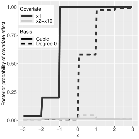
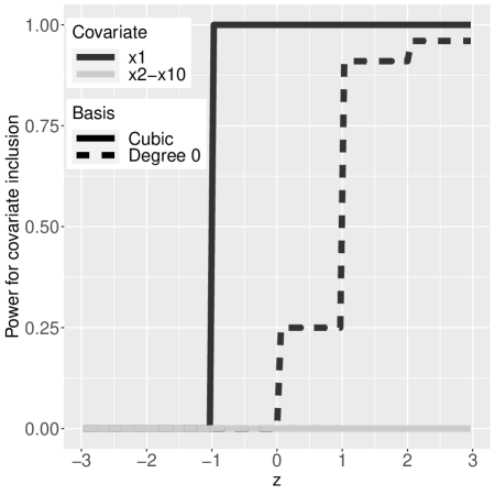
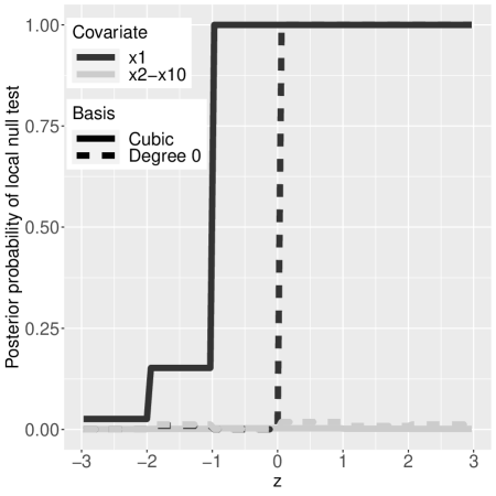
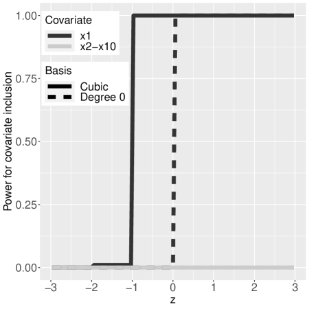
Figure 6. Simulated example. Posterior probability of local null test and proportion of rejected null hypotheses. Top: $n=100$. Bottom: $n=1,000$

	Cut degree 0	Cubic B-splines	VC-BART
$n=100$	0.173	0.168	0.241
$n=1000$	0.063	0.078	0.168

Table 3. Independent errors simulation. Root Mean Squared Error $E_{F}\left[\hat{E}(y_{i})-E_{F}(y_{i})\right]^{2}$ for 0-degree cut splines, cubic B-splines and VC-BART

We outline supplementary results for the simulation study presented in Section 5.1 of the main manuscript. Table 2 shows type I error and power (across 100 simulations) for the various considered methods. Figure 6 shows the posterior probability (average across 100 simulations) for the presence of a covariate effect as a function of $z$. Covariate 1 is truly active for $z>0$ and inactive for $z\leq 0$, covariates 2-10 are truly inactive at any $z\in[-3,3]$.

Table 3 displays the root mean squared error for the various considered methods.

$M=50$ individuals
Region	Covariate 1	Covariates 2-10
$z\in$(-3,-2]	0.06	0.080
$z\in$(-2,-1]	0.06	0.078
$z\in$(-1,0]	0.056	0.072
$z\in$(0,1]	0.73	0.084
$z\in$(1,2]	0.873	0.070
$z\in$(2,3]	1	0.057
$M=100$ individuals
Region	Covariate 1	Covariates 2-10
$z\in$ (-3,-2]	0.05	0.036
$z\in$ (-2,-1]	0.045	0.038
$z\in$ (-1,0]	0.0376	0.039
$z\in$ (0,1]	0.99	0.036
$z\in$ (1,2]	0.995	0.031
$z\in$ (2,3]	1	0.027

Table 4. Functional data simulation. Proportion of rejected null hypothesis for 0-degree cut orthogonal basis. For covariate 1 and $z>0$ this is the statistical power, otherwise it is the type I error

17.2. Functional data simulation

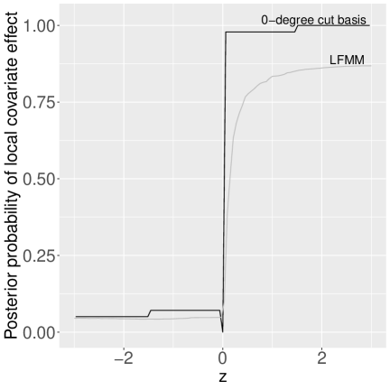
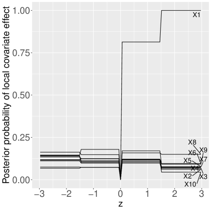
Figure 7. Functional data simulation. Posterior probability of a local covariate effect when using a single covariate (left) and 10 covariates (right)

Figure 7 displays a comparison of the two Bayesian methods, our framework and LFMM proposed by Paulon et al. (2023), in terms of the posterior probability assigned to the existence of a local covariate effect as a function of $z$ (averaged across 100 simulations). The left panel is based on fitting the model where one only consider the truly active covariate 1, whereas the right panel also includes truly spurious covariates 2-10. Recall that covariate 1 truly has an effect only for $z>0$.

17.3. Application to multi-electrode electrocorticography data

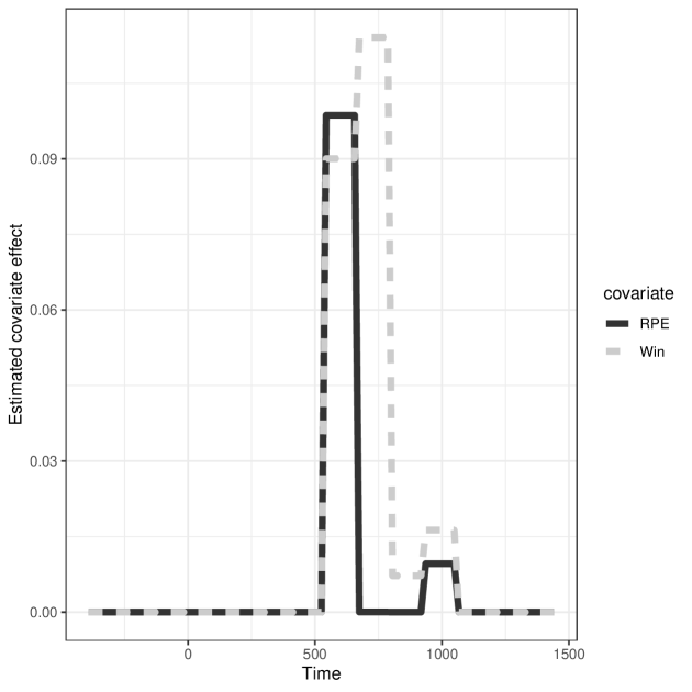
Figure 9. Estimated time-varying effects of two outcome-related covariates (Win, RPE) in the multi-variable analysis for the application of Section 5.4. The only relevant variable is RPE, with highest marginal probability of an effect $0.949$.

References

• Berger and Delampady (1987) Berger, J. O. and M. Delampady (1987). Testing precise hypotheses. Statistical Science 2(3), 317–352.
• Boehm Vock et al. (2015) Boehm Vock, L., B. Reich, M. Fuentes, and F. Dominici (2015). Spatial variable selection methods for investigating acute health effects of fine particulate matter components. Biometrics 71(1), 167–177.
• Caragea and Smith (2006) Caragea, P. and R. L. Smith (2006). Approximate likelihoods for spatial processes. Technical report, University of North Carolina at Chapel Hill.
• Castillo et al. (2015) Castillo, I., J. Schmidt-Hieber, and A. van der Vaart (2015). Bayesian linear regression with sparse priors. The Annals of Statistics 43(5), 1986–2018.
• Chen and Chen (2008) Chen, J. and Z. Chen (2008). Extended Bayesian information criteria for model selection with large model spaces. Biometrika 95(3), 759–771.
• Choi and Lawson (2018) Choi, J. and A. B. Lawson (2018). Bayesian spatially dependent variable selection for small area health modeling. Statistical methods in medical research 27(1), 234–249.
• Deshpande et al. (2020) Deshpande, S. K., R. Bai, C. Balocchi, and J. E. Starling (2020). VC-BART: Bayesian trees for varying coefficients. arXiv 2003.06416, 1–53.
• Flood et al. (2020) Flood, S., M. King, R. Rodgers, S. Ruggles, and J. R. Warren (2020). Integrated public use microdata series, current population survey: Version 7.0 [dataset]. Minneapolis, MN: IPUMS.
• Hastie and Tibshirani (1993) Hastie, T. and R. Tibshirani (1993). Varying-coefficient models. Journal of the Royal Statistical Society B 55(4), 757–796.
• Jhuang et al. (2019) Jhuang, A.-T., M. Fuentes, J. Jones, G. Esteves, C. Fancher, M. Furman, and B. Reich (2019). Spatial signal detection using continuous shrinkage priors. Technometrics 61(4), 494–506.
• Kang et al. (2018) Kang, J., B. Reich, and A.-M. Staicu (2018). Scalar-on-image regression via the soft-thresholded Gaussian process. Biometrika 105(1), 165–184.
• Morris et al. (2011) Morris, J. S., V. Baladandayuthapani, R. C. Herrick, P. Sanna, and H. Gutstein (2011). Automated analysis of quantitative image data using isomorphic functional mixed models, with application to proteomics data. The annals of applied statistics 5(2A), 894.
• Müller et al. (2004) Müller, P., G. Parmigiani, C. Robert, and J. Rousseau (2004). Optimal sample size for multiple testing: the case of gene expression microarrays. Journal of the American Statistical Association 99(468), 990–1001.
• Narisetty and He (2014) Narisetty, N. and X. He (2014). Bayesian variable selection with shrinking and diffusing priors. The Annals of Statistics 42(2), 789–817.
• Paulon et al. (2023) Paulon, G., P. Müller, and A. Sarkar (2023). Bayesian semiparametric hidden markov tensor models for time varying random partitions with local variable selection. Bayesian Analysis 1(1), 1–31.
• Pini and Vantini (2016) Pini, A. and S. Vantini (2016). The interval testing procedure: a general framework for inference in functional data analysis. Biometrics 72(3), 835–845.
• Rossell (2022) Rossell, D. (2022). Concentration of posterior model probabilities and normalized L0 criteria. Bayesian Analysis 17(2), 565–591.
• Rossell et al. (2021) Rossell, D., O. Abril, and A. Bhattacharya (2021). Approximate Laplace approximations for scalable model selection. Journal of the Royal Statistical Society B 83(4), 853–879.
• Rossell and Telesca (2017) Rossell, D. and D. Telesca (2017). Non-local priors for high-dimensional estimation. Journal of the American Statistical Association 112, 254–265.
• Saez et al. (2018) Saez, I., J. Lin, A. Stolk, E. Chang, J. Parvizi, G. Schalk, R. Knight, and M. Hsu (2018). Encoding of multiple reward-related computations in transient and sustained high-frequency activity in human ofc. Current Biology 28(18), 2889–2899.
• Scheel et al. (2013) Scheel, I., E. Ferkingstad, A. Frigessi, O. Haug, M. Hinnerichsen, and E. Meze-Hausken (2013). A Bayesian hierarchical model with spatial variable selection: the effect of weather on insurance claims. Journal of the Royal Statistical Society: Series C (Applied Statistics) 62(1), 85–100.
• Schwarz (1978) Schwarz, G. (1978). Estimating the dimension of a model. Annals of Statistics 6, 461–464.
• Scott and Berger (2006) Scott, J. and J. Berger (2006, July). An exploration of aspects of Bayesian multiple testing. Journal of Statistical Planning and Inference 136(7), 2144–2162.
• Smith and Fahrmeir (2007) Smith, M. and L. Fahrmeir (2007). Spatial Bayesian variable selection with application to functional magnetic resonance imaging. Journal of the American Statistical Association 102(478), 417–431.
• Varin et al. (2011) Varin, C., N. Reid, and D. Firth (2011). An overview of composite likelihood methods. Statistica Sinica 21(1), 5–42.
• Zhu et al. (2011) Zhu, H., P. J. Brown, and J. S. Morris (2011). Robust, adaptive functional regression in functional mixed model framework. Journal of the American Statistical Association 106(495), 1167–1179.