DISTINQT: A Distributed Privacy Aware Learning Framework for QoS Prediction for Future Mobile and Wireless Networks

Abstract

Beyond 5G and 6G networks are expected to support new and challenging use cases and applications that depend on a certain level of Quality of Service (QoS) to operate smoothly. Predicting the QoS in a timely manner is of high importance, especially for safety-critical applications as in the case of vehicular communications. Although until recent years the QoS prediction has been carried out by centralized Artificial Intelligence (AI) solutions, a number of privacy, computational, and operational concerns have emerged. Alternative solutions have been surfaced (e.g. Split Learning, Federated Learning), distributing AI tasks of reduced complexity across nodes, while preserving the privacy of the data. However, new challenges rise when it comes to scalable distributed learning approaches, taking into account the heterogeneous nature of future wireless networks. The current work proposes DISTINQT, a privacy-aware distributed learning framework for QoS prediction. Our framework supports multiple heterogeneous nodes, in terms of data types and model architectures, by sharing computations across them. This, enables the incorporation of diverse knowledge into a sole learning process that will enhance the robustness and generalization capabilities of the final QoS prediction model. DISTINQT also contributes to data privacy preservation by encoding any raw input data into a non-linear latent representation before any transmission. Evaluation results showcase that our framework achieves a statistically identical performance compared to its centralized version and an average performance improvement of up to 65% against six state-of-the-art centralized baseline solutions in the Tele-Operated Driving use case.

I Introduction

Forthcoming beyond 5G (B5G) and 6G network systems are expected to steer a new era of wireless mobile networks supporting new and challenging use cases and applications, such as autonomous vehicles, holographic communications, digital twins, pervasive intelligence and global ubiquitous connectability [1]. Such use cases will introduce new services involving heterogeneous data streams, devices, resources, operations, and entirely new Key Performance Indicators (KPIs) [2, 3]. The viability of these services is dependent on a certain level of Quality of Service (QoS) to operate smoothly and provide a satisfactory experience to end users. As such, there is a major requirement for mechanisms able to detect imminent changes in the QoS [4], and proceed to proactive service adaptation actions, ensuring an uninterrupted service operation. The QoS may be expressed in terms of the minimum required data rate, acceptable packet loss ratio, response time, and other related KPIs.

In parallel, the use of Artificial Intelligence (AI) has been recognized as a key enabler in future wireless networks by both Industry and Academia [5]. So far, mainly centralized AI approaches [6, 7, 8, 9, 10, 11] have been employed for QoS prediction, requiring data transfers from source devices to centrally located data centers and, thus, suffering from data privacy, computational complexity and operational costs [12]. Alternative AI solutions have also recently been emerged (e.g. Split Learning, Federated Learning), distributing AI related tasks of reduced computational complexity (e.g. local training) to a number of (in general heterogeneous) devices, while exploiting locally stored datasets and avoiding any raw data exchanges [13].

The 3rd Generation Partnership Project’s (3GPP) in Rel. 18, attempts to adopt distributed learning by introducing multiple distributed Network Data Analytics Functions (NWDAFs) [14], incorporating the Model Training Logical Function (MTLF) [15]. Concurrently, 3GPP’s Rel. 19, investigates new deployment and management options, as well as new functionality and KPI requirements that enable model transfer, which is of significant importance in the context of distributed learning [16].

The benefits of distributed learning are well understood but can be gained as long as some significant challenges are addressed, related to distributing AI in wireless networks. One of the major challenges towards an effective learning is factoring in device heterogeneity, in terms of data types, data distribution, and computational capabilities; model heterogeneity may also be present due to possible variations in model architectural options. The challenge in this case is to strike a good balance between the level of integration of heterogeneous model architectures and learning effectiveness. The latter necessitates the investigation for model aggregation techniques capable of producing robust and well performing models, especially in cases of critical services and applications with stringent QoS requirements [17]. In addition, ways to cope with the anticipated increased burden on network resources are needed: distributed learning typically requires continuous model update transmissions, comprising millions or even billions of model parameters, a burden that increases proportionally to the number of devices participating in the distributed AI mechanism.

In view of the limitations of centralized QoS prediction approaches and the challenges in deploying effectively distributed learning, it becomes apparent that new and innovative solutions are required for QoS prediction in future mobile networks. Such solutions should enable a scalable distributed learning execution across heterogeneous network entities and model architectures, while contributing to privacy preservation and ensuring a robust model performance.

Although distributed learning has gained significant attention, only a limited number of state-of-the-art works propose its application to predicting QoS [18, 19, 20]. These works apply federated learning techniques assuming identical data types and Neural Network (NN) architectures across the nodes, allowing for differences only in data distribution and size. However, heterogeneous environments are not uncommon, where different types of data may be collected by different network nodes, also requiring different NN architectures to extract meaningful insights related to the prediction task. Such heterogeneous environments cannot be addressed by the past works and are considered in this paper.

Motivated by these open challenges, the current work proposes DISTINQT, a novel privacy-aware distributed learning framework based on sequence-to-sequence autoencoders [21], capable of providing accurate predictions to end users for a future time horizon. More specifically, the DISTINQT’s architecture extends upon our previous work [22], preserving data privacy by distributing (among distinct nodes) a number of NN-Encoders, capable of encoding input data into a non-linear latent representation before any transmission. DISTINQT also allows different architectural options for each NN-Encoder, depending on the data types collected at the different nodes. This flexibility enables the incorporation of diverse knowledge and model architectures into a sole learning process that will enhance the robustness and generalization capabilities of the final QoS prediction model.

The key contributions can be summarized as follows:

• We propose a distributed learning framework for QoS prediction, sharing computations of lower complexity among different nodes, training a complex NN model.

• Our distributed framework is able to support network entities with similar and heterogeneous characteristics, both in terms of data types and model architectures. As such, our framework captures diverse knowledge towards a robust and generalized model for QoS prediction.

• Our framework is privacy-aware, contributing to data privacy preservation by encoding raw input data into a non-linear latent representation before any transmission.

The rest of the paper is organized as follows. Section II presents relevant state-of-the-art works. Section III provides an extensive description of our proposed distributed framework that is evaluated in the Tele-operated Driving use case described in Section IV, where the performance evaluation results are provided in Section V. Finally, section VI concludes the paper.

II Related Work

This section provides an overview of the literature regarding distributed learning approaches for wireless networks, targeting also the QoS prediction. Despite the fact that the concept of distributed learning has become compelling, its application in various open challenges for future wireless networks is still at a rather early stage.

A number of related works study different NN architectural options for distributed and federated learning. The authors of [23] provide a comprehensive survey on definitions, architectures, and applications for the federated-learning framework. In [24] the authors propose a mobility vertical federated forecasting framework that allows the learning process to be jointly conducted over vertically partitioned data belonging to multiple organizations. Another work [25] introduces the concept of split learning, reviews traditional, novel, and state-of-the-art split learning methods, and discusses current challenges and trends. The [26] proposes a privacy-sensitive parallel split Learning method that prevents overfitting considering the differences in a training order and data size at each node. Kim et.al [27] propose a novel spatio-temporal split learning framework with multiple end-systems, in order to realize privacy-preserving Deep Neural Network (DNN) computation. The work [28] proposes an edge-enabled distributed deep learning platform by dividing a general DNN into a front and back subnetwork. The front subnetwork is deployed close to input data, trained at each edge device and all produced outputs are sent to the back subnetwork for later training at a cloud center.

There is also a number of works related to the application of distributed learning in wireless networks for a variety of use cases including computational offloading, model partitioning and energy efficiency. In works [29] and [30] the authors propose a fine-grained adaptive partitioning scheme to divide a source DNN in partitions. Two integrating options are proposed including a local execution at an end device, or partition offloading to one or multiple powerful nodes. Another work [31] investigates DNN inference offloading in a 5G environment, aiming to increase the prediction request acceptance or to minimize the energy consumption of edge devices. Zeng et. al [32], propose CoEdge, a distributed DNN computing system that orchestrates cooperative prediction over heterogeneous edge devices towards minimizing the system energy consumption while promising response latency requirement. In another work [33] the authors propose DeCNN, a prediction approach that uses decoupled Convolutional NN (CNN) structure to optimize multi-level parallelism for distributed prediction on end devices. Additionally in [34], the authors propose DeepHome, a framework that can distribute NN inference tasks to multiple heterogeneous devices inside a home.

Finally, only a limited number of works focus on the application of distributed learning for QoS prediction in mobile networks. Zhang et.al [18] propose a privacy-preserving QoS prediction, leveraging federated learning techniques, along with several efficiency improvements to reduce system overhead. The authors in [19] propose MultiFed, which is a multi-centre FL framework for QoS prediction via a cloud–edge collaboration mechanism. The work in [20] discusses a personalized federated tensor factorization framework for distributed privacy-preserving IoT services QoS prediction. However, these works assume identical data types and NN architectures across nodes, while considering differences only in data distribution and size.

As already stated in the Introduction, there is a gap in the state-of-the-art works when it comes to distributed learning approaches for QoS prediction taking into account both common and heterogeneous nodes, in terms of data types and model architectures, along with data privacy and knowledge sharing. The current work extends [22], by enabling the distribution of the learning apart from the inference/prediction process. DISTINQT is the first one that proposes a distributed learning framework for QoS prediction, sharing computations of lower complexity among different nodes across the network, supporting network entities with similar and heterogeneous data types and model architectures. Our framework contributes to data privacy preservation by encoding raw input data into a non-linear latent representation before any transmission.

III DISTINQT Framework

This section provides an extensive description of the DISTINQT framework towards a privacy preserving distributed learning scheme for QoS prediction. DISTINQT could be effectively applied to any wireless network environment comprised of distinct types of Network Entities (NETs), such as UE, BS, MEC, Cloud etc. DISTINQT follows an hierarchical structure, enabling distibuted learning in large-scale network environments. Let $E$ denote the number of distinct NETs. Each NET $e\in\{1,...,E\}$ may be comprised of multiple workers. All workers of a specific NET share the same input features (data types) but the number and distribution of data samples may differ. However, workers of different NETs collect and process different input features related with a learning task.

III-A Role Assignment

The DISTINQT framework is realized in a synchronized manner and is capable of providing QoS predictions for a specific time horizon. At the beginning of the learning phase, each NET is assigned with one of the following roles:
Active NET: An active NET holds data samples related with the learning task, as well as the set of groundtruth data (i.e. QoS KPI). Only one NET can be assigned this role.
Passive NET: A passive NET holds data samples related with the learning task, without any groundtruth data. Multiple NETs can be passive.
Local NET Aggregator: A local aggregator is assigned to each NET, acting as an intermediate point in the distributed forward and backpropagation processes, by collecting and transmitting all the necessary inputs, aggregating and updating the trainable weights of the involved workers of a specific NET.
Coordinator NET: A coordinator NET coordinates the learning process in a synchronized manner, by contributing to the learning process with its own data samples, while also orchestrating the communication of the involved NETs. In our setting, the role of the coordinator is assigned to the active NET $c$, $c\in\{1,...,E\}$.

III-B Neural Network Architecture and Distribution

Fig. 1 depicts a high level overview of the DISTINQT’s NN architecture that will be distributed among all involved workers of different NETs. The DISTINQT framework is based on sequence-to-sequence Autoencoder NN architectures [21, 35, 36, 37], designed to encode an input sequence into a compressed representation. Apart from the inherent dimensionality reduction, these architectures also contribute to privacy preservation, by encoding the initial raw data before any transmission.

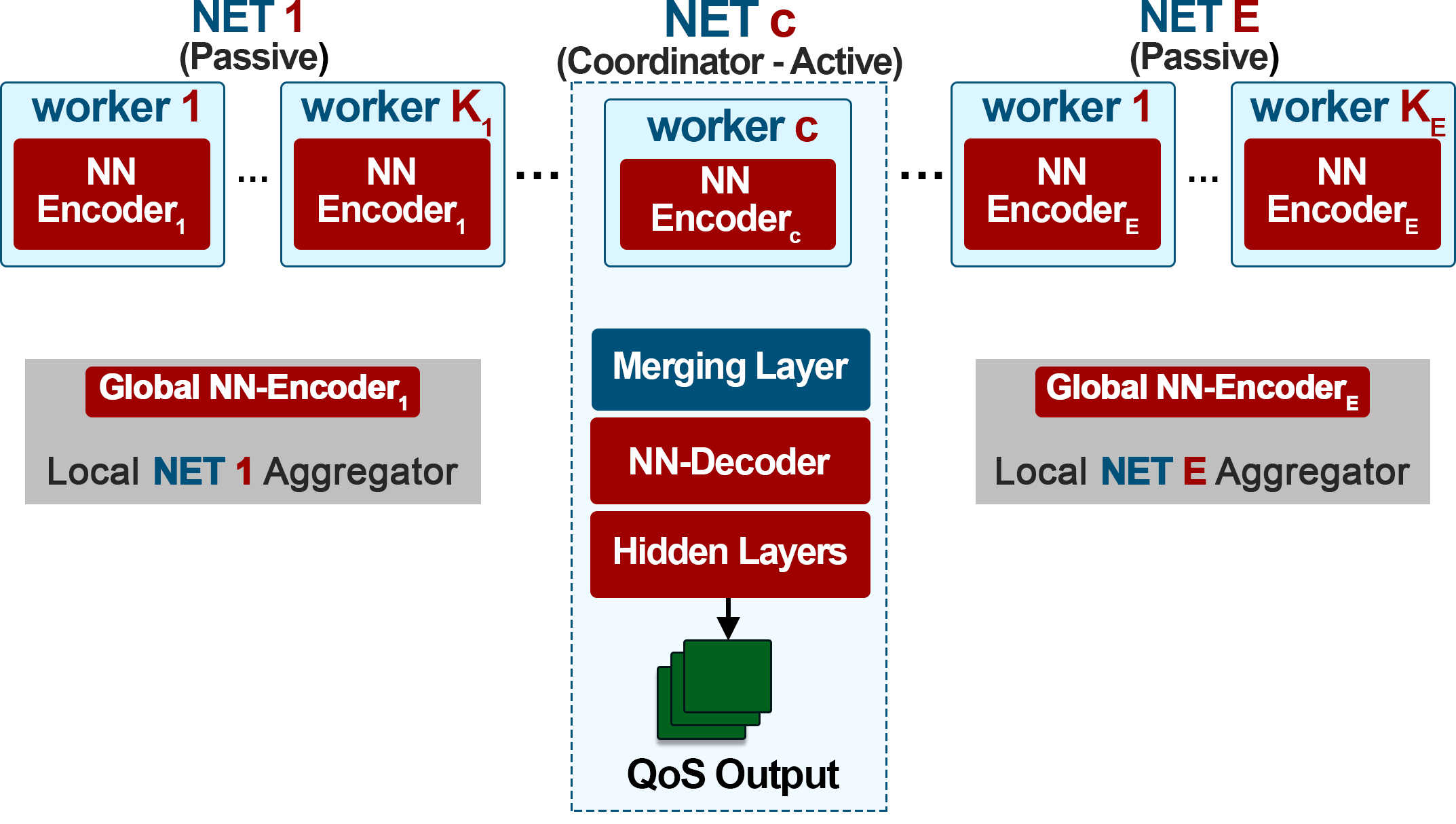
Figure 1: DISTINQT’s Architecture Overview

The structure of the DISTINQT’s NN architecture (NN model layers) is as follows:
NN-Encoder: Each worker is equipped with one NN-Encoder. Let $\mathsf{K}_{e}$ denote the total number of workers of NET $e$, $N_{enc}=\sum_{e=1}^{E}\mathsf{K}_{e}$ denote the total number of NN-Encoders in the system. Each NN-Encoder may be comprised of multiple encoding layers. An NN-Encoder processes an input sequence and encodes it into a fixed-length vector, named as context vector, while applying a non-linear activation function (e.g. the rectified linear activation function - ReLU). This preserves data privacy, since the mapping of the input sequence to a non-linear latent representation is of higher complexity and as such cannot be easily reversed by any other worker or snooper [38, 39]. The workers of the same NET employ identical NN-Encoders, in terms of number and type of encoding layers, as well as number of neurons per layer. Indicative examples of such NN-Encoder types include: Long-Short Term Memory, Transformer, Convolutional encoders etc. The NN-Encoders used by distinct NETs may differ in their NN structure, depending on the use case, data types (e.g. visual, aural, numerical), and computational capabilities of the workers. DISTINQT’s flexibility in architecture configuration could enable and support a multi-modal learning process [40].

The rest of the NN architecture is located at the coordinator NET (NET $c$) and includes a Merging Layer, an NN-Decoder, as well as a number of Hidden Layers.
Merging Layer: This layer is responsible for applying a merging function (e.g. summation, concatenation, average) to the context vectors produced by all workers, including the coordinator. The merging is performed between interconnected (associated) workers resided on different NETs (more details in Section III-C).
NN-Decoder: The NN-Decoder is responsible for constructing the future sequence over the selected time horizon, based on the output of the Merging Layer. It should be noted that the NN-Decoder does not attempt to reconstruct any initial input sequence.
Hidden Layers: This part of the DISTINQT’s architecture includes a set of hidden layers (e.g. fully connected), where their number and type could vary, depending on the prediction task.
Global NN-Encoder: When all NN-Encoders of a NET are updated (trainable parameters), the respective Local NET Aggregator produces a global model update, named as Global NN-Encoder, by aggregating the updated trainable parameters of the corresponding NN-Encoders.

The Global NN-Encoder can integrate collective and heterogeneous knowledge from the participating workers, enhancing the performance, convergence speed and the generalization capabilities of our proposed framework. The latter relies on the fact that workers with limited amount of data could benefit from others with more diverse datasets. Diverse datasets frequently lead to more resilient parameter updates for the NN-Encoders that could increase the knowledge base of others with insufficient data samples in a collaborative manner (parameter aggregation).

In addition, the Global NN-Encoder also enables a seamless and effective inclusion of additional workers throughout the learning process. More specifically, if a new worker of a NET $e$ requests to participate, the responsible Local NET Aggregator will provide the latest update of the Global NN-Encoder and the new worker will join the process. In any other case, a newly added worker with a newly instantiated NN-Encoder could introduce noise in the learning process.

III-C Methodology

Figs. 2 and 5 illustrate the logical steps of the DISTINQT framework. These steps are repeated for multiple rounds (epochs) until convergence and are synchronized by the coordinator NET. Each epoch consists of multiple batch loops. In each batch loop $b$, two well-known types of processes take place, namely the forward (inference/prediction) and backward (learning) pass process. Multiple forward pass and one backward pass processes are executed during a batch loop. In each forward pass, an input feature sequence is fed through the NN in a forward direction, yielding calculations of intermediate variables and eventually generating a prediction (model output). At the end of a batch loop, a backward pass is initiated. The backward pass involves the calculations of the gradients of the loss function w.r.t the trainable parameters of each NN layer of the DISTINQT architecture by recursively applying the chain rule to update the parameters in order to minimize the loss [41].

DISTINQT’s learning procedure can be divided into nine logical steps. A complete notation table is given in Table I.
Forward Pass (Fig. 2):
Step \raisebox{-.9pt} {1}⃝: Each worker periodically collects a sequence of input features. The logging frequency of the input features $\tau_{e}$ ($e\in\{1,...,E\}$) may vary per NET and it is expressed through a discrete time unit, the timestep. In each batch loop $b$, all NN-Encoders process a batch $B$ of input sequences. The batch size $s$ is selected by NET $c$, based on the prediction task, and it is the same for all workers. Each input sequence initiates a forward pass process. This sequence includes historical features for $h_{e}$ consecutive past timesteps, comprising a historical time horizon with duration $H_{e}$ ($H_{e}=h_{e}\cdot\tau_{e}$).

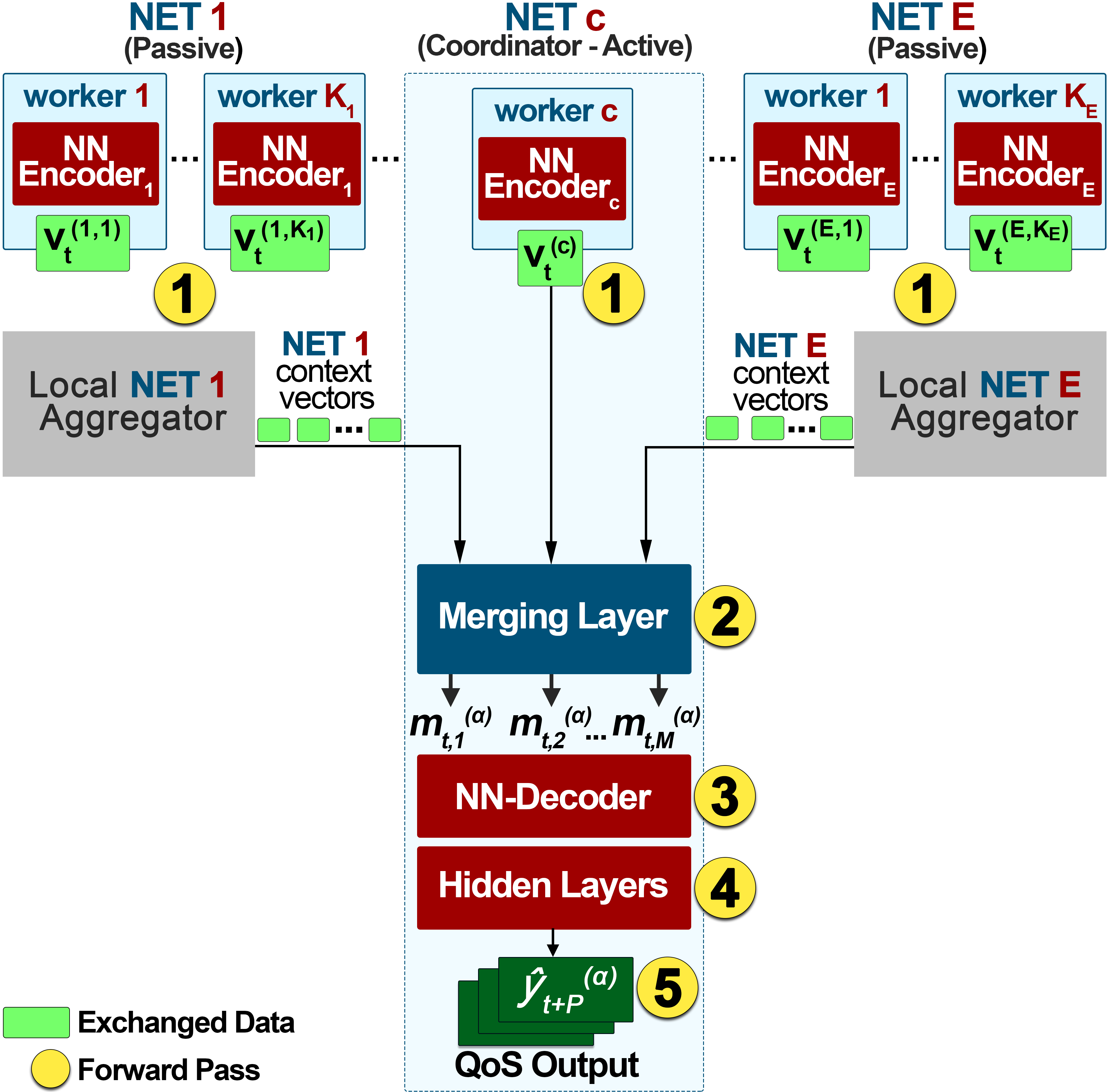
Figure 2: DISTINQT’s Forward Pass

Let $t$ denote the timestep when all workers encode their input sequence into a context vector. We assume that the selection of $t$ is performed by the coordinator and should be greater or equal than the maximum logging frequency of all workers ($t\geq\tau_{e},\forall e\in\{1,...,E\}$). This condition ensures that all workers produce context vectors only when new data samples are available, avoiding waste of resources. Let $N_{e}$ denote the common dimensionality (length) of the context vector of all workers of NET $e$. Let $\nu^{(e,k)}_{t,i}$, $i\in\{1,...,N_{e}\}$, denote the $i^{th}$ element of the context vector of worker $k$ of NET $e$ at timestep $t$. Let $\textbf{v}^{(e,k)}_{t}=[\nu^{(e,k)}_{t,1},\nu^{(e,k)}_{t,2},...,\nu^{(e,k)}_{t,N_{e}}]^{T}$ denote the context vector of worker $k$ of NET $e$ at timestep $t$. We assume that each NET worker produces a non-zero context vector at each timestep $t$ ($\textbf{v}^{(e,k)}_{t}\neq\textbf{0}$). The context vectors of all passive NETs are collected by the responsible Local NET Aggregators to transmit them to NET $c$.
Step \raisebox{-.9pt} {2}⃝: This step includes the merging of the context vectors that is performed by the coordinator NET, which keeps track of the interconnections. The merging is realized only among the interconnected workers of different NETs. As an example, consider a wireless mobile network of three NETs, namely a UE, a BS, and a MEC, with three, two and one workers of each type, shown in Fig. 3. The different line colors indicate the different interconnections (three in total). The MEC worker acts as the coordinator. Fig. 4 maps this wireless network to DISTINQT and illustrates the merging process. The context vector of each UE worker will be merged with the context vector of the connected (associated) BS worker and consequently with the context vector of the associated (to the respective BS) MEC-worker. As a result three merged vectors will be produced by applying a merging function to the following vectors: [$\textbf{v}_{t}^{(\textrm{UE},1)}$, $\textbf{v}_{t}^{(\textrm{BS},1)}$, $\textbf{v}_{t}^{(\textrm{MEC},1)}$], [$\textbf{v}_{t}^{(\textrm{UE},2)}$, $\textbf{v}_{t}^{(\textrm{BS},1)}$, $\textbf{v}_{t}^{(\textrm{MEC},1)}$], [$\textbf{v}_{t}^{(\textrm{UE},3)}$, $\textbf{v}_{t}^{(\textrm{BS},2)}$, $\textbf{v}_{t}^{(\textrm{MEC},1)}$].

Figure 3: Example of three interconnections in a Wireless Mobile Network

Figure 4: Example of DISTINQT’s Merging Process

Let $A_{t}$ denote the total number of merged vectors produced by the merging layer at timestep $t$. All merged vectors are of the same length, denoted by $M$. Let $m_{t,i}^{(a)}$ with $a\in\{1,...,A_{t}\}$ and $i\in\{1,...,M\}$, denote the $i^{th}$ element of the merged vector of interconnection $a$ at timestep $t$. Consequently, the output of the merging layer, associated with interconnection $a$, is the vector $\textbf{m}^{(a)}_{t}=[m_{t,1}^{(a)},...,m_{t,M}^{(a)}]^{T}$. In the example given by Fig. 4, the produced merged vectors are the $\textbf{m}^{(1)}_{t}$, $\textbf{m}^{(2)}_{t}$ and $\textbf{m}^{(3)}_{t}$.
Steps \raisebox{-.9pt} {3}⃝-\raisebox{-.9pt} {5}⃝: For each interconnection $a$, the merged vector $\textbf{m}^{(t)}_{a}$ is provided as input to the NN-Decoder. As mentioned, the NN-Decoder constructs the future sequence of the selected prediction time horizon $\mathsf{P}$ ($\mathsf{P}=p\cdot\uptau_{c}$) and it is comprised of $p$ prediction horizon timesteps in total. This prediction horizon timestep is selected by the coordinator and is denoted by $\uptau_{c}$.

$E$	Number of distinct NETs
$\mathsf{K}_{e}$	Number of workers of NET $e$
$B$	Batch of input sequences
$b$	Batch loop
$s$	Batch size
$\tau_{e}$	Logging frequency timestep of NET $e$
$\uptau_{c}$	Prediction horizon timestep selected by NET $c$
$t$	Timestep of the current forward pass
$h_{e}$	Number of timesteps in a historical time horizon $H_{e}$
$p$	Number of timesteps in a prediction time horizon $\mathsf{P}$
$H_{e}$	Duration of historical time horizon of NET $e$
$\mathsf{P}$	Duration of the prediction time horizon
$N_{enc}$	Total number of Encoding layers (NN-Encoders)
$N_{e}$	Length of the context vector of NET $e$
$\nu^{(e,k)}_{t,i}$	The $i^{th}$ element of the context vector of worker $k$ of NET $e$ at timestep $t$
$\textbf{v}^{(e,k)}_{t}$	Context vector of worker $k$ of NET $e$ at timestep $t$
$\textbf{v}^{(c)}_{t}$	Context vector of coordinator $c$ at timestep $t$
$A_{t}$	Total number of merged vectors at timestep $t$
$M$	Length of the merged vector
$m_{t,i}^{(a)}$	The $i^{th}$ element of the merged vector of interconnection $a$ at timestep $t$
$\textbf{m}^{(a)}_{t}$	Vector output of the merging layer
$\hat{\textbf{y}}^{(a)}_{t}$	Predicted output sequence of interconnection $a$ at timestep $t$
$\hat{\textbf{y}}_{b}$	Set of predicted output sequences at batch loop $b$
$\textbf{w}_{b}^{(e,k)}$	The weight updates of worker $k$ of NET $e$ at batch loop $b$
$\textbf{w}_{b}^{(e)}$	Aggregated trainable weights of NET $e$ at batch loop $b$

TABLE I: Notation Table

The output of the NN-Decoder feeds the next Hidden Layers. The final output is a sequence of the selected QoS KPI over the $p$ future timesteps, denoted as $\hat{\textbf{y}}^{(a)}_{t}=[\hat{y}^{(a)}_{(t+\tau)},...,\hat{y}^{(a)}_{(t+p\cdot\uptau_{c})}]^{T}$. The set of outputs produced at batch loop $b$ is defined as $\hat{\textbf{y}}_{b}=\{\hat{\textbf{y}}^{(a)}_{t},\forall t\in B,\forall a\}$ and its size is equal to $s\times a$.
Backward Pass (Fig. 5):

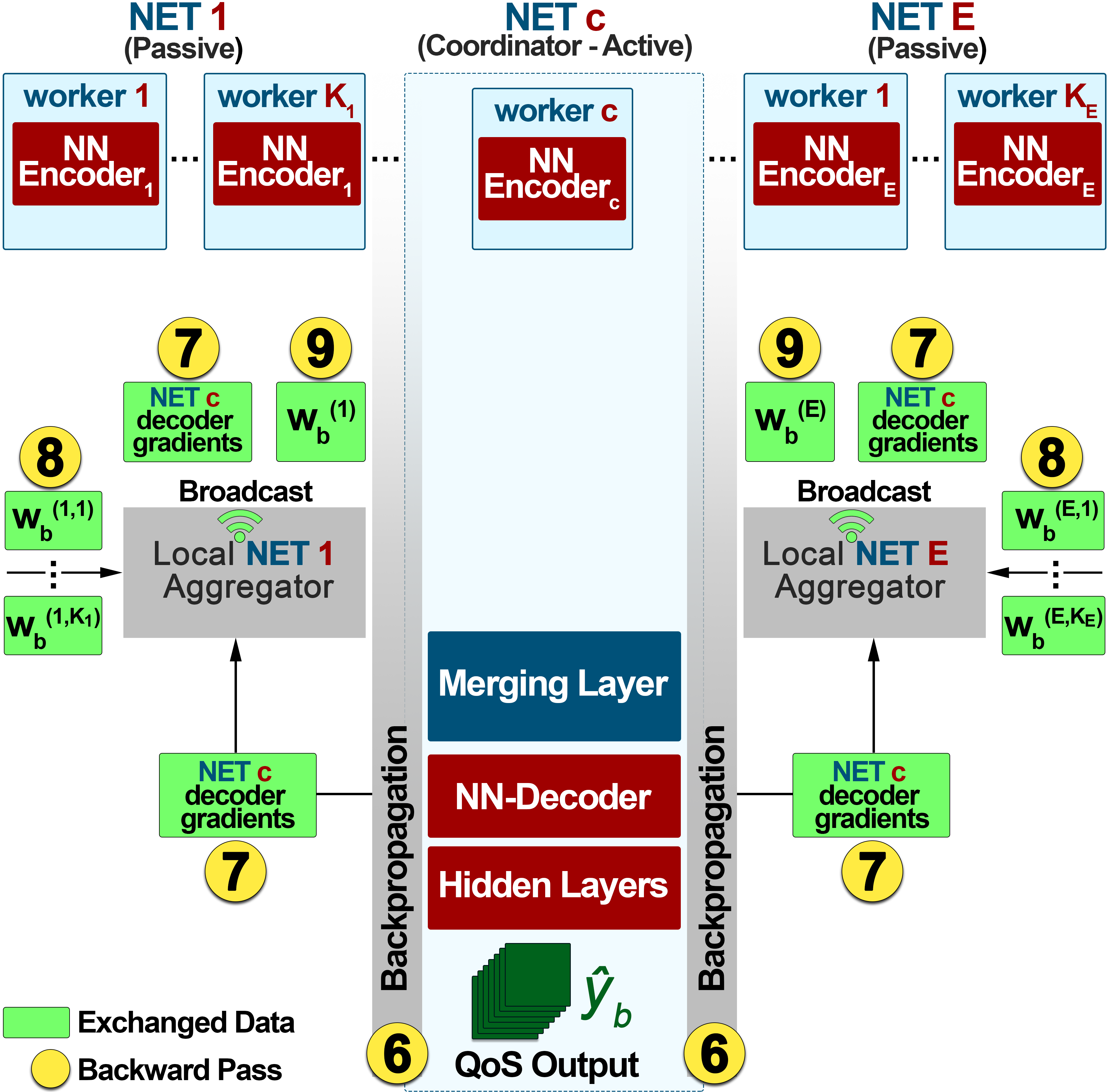
Figure 5: DISTINQT’s Backward Pass

Step \raisebox{-.9pt} {6}⃝: Once the forward pass processes of batch loop $b$ are complete, the predicted output sequence $\hat{\textbf{y}}_{b}$ along with the groundtruth sequence will be used, in order to minimize the loss function of the DISTINQT framework and perform the backpropagation process. During the backpropagation, the gradients of each layer (partial derivatives of the loss function w.r.t the trainable parameters) are computed by recursively applying the chain rule up to the NN-Encoder of worker $c$. The computed gradients will be used in order to update the trainable weights of worker $c$.
Step \raisebox{-.9pt} {7}⃝: The computed gradients of the NN-decoder are forwarded to the Local NET Aggregators of the involved NETs to continue a distributed backpropagation process. The Local NET Aggregators broadcast the received gradients to the workers of the associated NET to update their trainable weights using their own optimizers. Let $\textbf{w}_{b}^{(e,k)}$ denote the weight updates of worker $k$ of NET $e$ at the end of batch loop $b$.
Step \raisebox{-.9pt} {8}⃝: All workers send their updated weights to the respective Local NET Aggregator for aggregation based on an averaging function. The Local NET Aggregator of each NET $e$ updates the Global NN-Encoder with the aggregated weights $\textbf{w}_{b}^{(e)}$, given by:

$$\textbf{w}_{b}^{(e)}=\frac{\sum_{k=1}^{\mathsf{K}_{e}}\textbf{w}_{b}^{(e,k)}}{\mathsf{K}_{e}}\vspace{-8pt}$$ (1)

Step \raisebox{-.9pt} {9}⃝: The Local NET Aggregator broadcasts the aggregated trainable weights $\textbf{w}_{b}^{(e)}$ back to the respective workers to update their NN-Encoder. This step completes a batch loop of the learning process. It should be noted that after this step, all workers of a NET will have the same NN-Encoder, i.e. same trainable weights.
Steps \raisebox{-.9pt} {1}⃝-\raisebox{-.9pt} {9}⃝ are repeated for each batch loop and for each epoch of the learning process until convergence.

Finally, it should be mentioned that since the learning process is repeated for each batch loop, it could potentially lead to an increase in the communication overhead. This overhead could be potentially mitigated by applying effective compression techniques for NNs, such as connection pruning, weight quantization, knowledge distillation [42]. However, since this aspect is not covered in this work, we assume that there are no strict limitations in communication resources.

IV DISTINQT in Tele-Operated Driving

The current section presents the Tele-Operated Driving (ToD), [43], and simulation environments used in the evaluation of the DISTINQT framework, along with the considered configuration setups. The proposed DISTINQT framework will be applied in order to predict the uplink throughput of a ToD-UE over a future time horizon; this time horizon is set equal to 20 secs for the derivation of the results presented in the next sections.

IV-A Configuration Setup

Network Environment: The discrete event network simulator (NS3) [44] has been used for the performance evaluation of the DISTINQT framework. The simulated topologies and the evaluation methodology chosen for this study are in line with the 3GPP’s guidelines [45], [46]. The duration of the simulation is equal to 280 minutes, while the logging frequency of the data is equal to $\tau_{e}=200$ milliseconds (ms) for all NETs in our study. Two types of UEs are considered in the simulation, namely ToD-UE and NonToD-UE vehicles, one BS and one MEC server. According to [47], the periodic traffic of the ToD-UEs is set to 20 Mbps for the uplink and 500 Kbps for the downlink. On the other hand, the NonToD-UEs generate periodic background traffic load that interferes with that from the ToD-UE vehicles and will impact on the latter’s QoS. The number of NonToD-UEs varies over time and is randomly selected in the range of $[0,100]$. Each NonToD-UE generates traffic of 4 Mbps for the uplink and 8 Kbps for the downlink, considered to be constant throughout the experiments. The mobility of all UEs was generated using the Simulation of Urban Mobility tool (SUMO) [48]. The ToD-UEs are moving continuously with a variable speed in the range of $(0,14]$ m/s corresponding to $(0,50]$ km/h, while the NonToD-UEs follow randomly generated trajectories inside the simulated topology, as provided by SUMO. We consider 10 simulated experiments, differing in the total background traffic load (depending on the number of NonToD-UEs) and the mobility patterns of the UEs. Table II summarizes the NS-3 parameters used in the simulated scenario.

Parameter Description	Default Value
No. of ToD-UES & BSs & MECs	5 & 1 & 1
No. of NonToD-UES	[0, 100]
UE & BS Transmission Power	23 dBm & 40 dBm
BS Center Frequency	2160 MHz
BS Downlink and Uplink Bandwidth	20 MHz
BS and UE antenna model type	1x Isotropic
Propagation Loss Model for LOS/NLOS	ITU-R P.1411

TABLE II: Network Simulation Parameters

Input Feature Configuration: Three distinct NETs are considered in this work, namely the ToD-UE, the BS and the MEC Server. The ToD-UE NET is comprised of 5 workers (one for each of the 5 ToD-UEs), while the BS and the MEC server have 1 worker each. The BS is an active NET (i.e., holds the groundtruth) and also the Coordinator NET (i.e., coordinating the learning process). The rest of the NETs are passive. The set of input features for QoS prediction collected at each NET, are listed below:
ToD-UE NET:

• location of the ToD-UE (latitude, longitude)

• speed of the ToD-UE in $m/s$

• distance of the ToD-UE from BS in $m$

• future location of the ToD-UE at the end of the selected prediction time horizon (latitude, longitude)

BS NET:

• BS traffic load, in terms of used Resource Blocks

• number of vehicles connected to the BS, in which the ToD-UE is attached to

• uplink SINR of the ToD-UE in $dBm$

• uplink throughput of the ToD-UE in $Mbps$

MEC Server NET:

• number of vehicles attached to neighboring BSs

• traffic load, in terms of used Resource Blocks, of neighboring BSs

We consider two distinct configuration setups, as listed in Table III. Configuration c1 includes solely the input features from the ToD-UE and the BS. Configuration c2 includes the input features of all considered NETs (i.e. also the MEC server NET). These configurations are specifically selected to demonstrate the applicability and the model performance of our DISTINQT framework, as a higher number of (heterogeneous) NETs are collaboratively involved in the learning process.

Configuration	Input Features
c1	ToD-UE $+$ BS
c2	ToD-UE $+$ BS $+$ MEC Server

TABLE III: Input Feature Configuration

DISTINQT’s Architecture Configuration: For the selected ToD use case, the architecture of the DISTINQT framework incorporates a Bidirectional Long Short Term Memory (BiLSTM) Layer as an NN-Encoder, a Concatenation Layer for merging, an LSTM NN-Decoder, followed by a Fully Connected (FC) Hidden Layer. For each configuration, the DISTINQT’s related parameters were optimized by exploiting a custom grid search method, with over 200 combinations of different model parameters. The selected parameters include: number of neurons per layer, L2 (weight decay) regularizer [41], activation function (AF) per layer, type of optimizer, learning rate (lr) and batch size. With respect to the evaluation metrics explained and provided in Section V, the best scored parameter combination of the DISTINQT’s architecture for c1 and c2 configurations is shown in Table IV. The best scored parameter combination yielded NN-Encoders with the same number of neurons for all workers. To keep the presentation simple, the ”Neurons” parameter shown in Table IV has the following form: {NN-Encoder} x {NN-Decoder} x {FC}.

Parameter	c1	c2
Neurons	100x200x200	100x200x100
L2	1e-06	1e-08
AF (All Layers)	ReLU
Optimizer & lr	Adam & 1e-03	Adam & 5e-05
Batch Size $s$	64

TABLE IV: DISTINQT’s Configuration Parameters: c1 & c2

The maximum number of epochs for the learning phase was set to 1000. Additionally, in order to avoid overfitting and potential degradation in the performance of the model, an early stopping function is applied, which monitors the Mean Squared Error (MSE) of the validation set [49]. As a result, the learning process stops, when the MSE score does not improve or starts deteriorating.

V Performance Evaluation

In the selected ToD use case, the DISTINQT framework is applied in order to predict the uplink throughput of a ToD-UE over a prediction (future) time horizon of $\mathsf{P}=20$ secs. The historical time horizon of monitored features, which are inputs to DISTINQT, is set to $H_{e}=25$ secs for all NETs; after a thorough experimentation, this value was determined to yield the best performance. For the learning phase, each NET uses 3280 seconds of input data. In the evaluation study, the prediction process moves forward in time in steps of size $t$ secs. That is, every $t=1$ sec the framework provides the predicted uplink throughput for the next prediction horizon. The proposed DISTINQT was evaluated by employing the Mean Absolute Error (MAE) metric (in Mbps), supplemented by its standard deviation, [50], based on 10 different evaluation scenarios (ES) per ToD-UE (50 ESs in total) under diverse background traffic load levels, with a mean simulation duration equal to $\sim$1116 seconds. These scenarios were selected to assess the robustness of our framework, under different network traffic conditions. The MAE score is calculated for each prediction horizon timestep ($\tau_{c}=200$ ms in our study for all types of NETs) and for all prediction time windows. Each prediction time window consists of $\frac{\mathsf{P}\text{(ms)}}{\tau_{c}}=p$ prediction timesteps, where $p=\frac{20000}{200}=100$; these prediction timesteps associated with the current timestep, $t$, are given by the sequence ($\{t+200,t+400,...,t+20000\}$ in ms; the historical time window $H_{e}$ secs corresponds to $h_{e}$ = 125 timesteps of historical information.

V-A DISTINQT vs Centralized

We compare the performance of our DISTINQT framework with a centralized LSTM-based approach, introduced in our previous work [51]. Table V, presents the evaluation results as average values of the MAE score for both input feature configurations and for all evaluation scenarios (50 in total). Two types of evaluation metrics are considered: (a) The ”overall MAE” score, representing the average MAE score over all prediction horizon timesteps, and (b) the ”20th Second MAE” score, representing the average MAE score of the last prediction horizon timestep only. The results under both the centralized, [51], and our proposed DISTINQT approaches are statistically very similar, with the DISTINQT showcasing a marginally better performance of 7.75% on average for both configurations and types of scores considered. Also c2 improves upon c1 on average by 5.65% for both scores, highlighting the importance of the additional input features of the MEC Server NET. MAE scores capture the overall ability of the model to yield a relatively low prediction error under the DISTINQT and the centralized approaches, considering typical uplink throughput values of the ToD applications (10-50 Mbps), as indicated by the EU funded 5GCroCo project [17].

Avg. (Mbps) ($\pm$ STD)	Overall MAE	20th Second MAE
DISTINQT (c1)	0.554 ($\pm$1.578)	0.6854 ($\pm$1.4340)
Centralized (c1)	0.6358 ($\pm$1.795)	0.734 ($\pm$1.389)
DISTINQT (c2)	0.529 ($\pm$1.574)	0.6388 ($\pm$1.325)
Centralized (c2)	0.568 ($\pm$1.667)	0.6702 ($\pm$1.303)

TABLE V: DISTINQT vs Centralized QoS prediction performance for input feature configurations c1 & c2

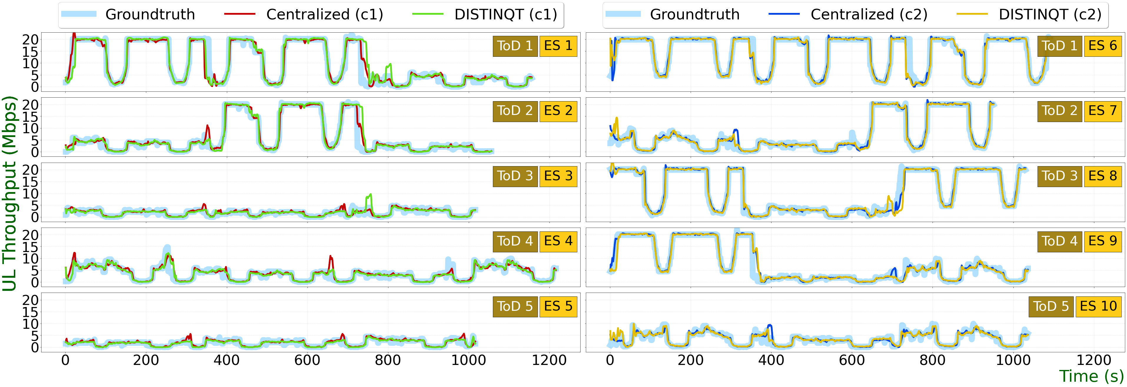
Figure 6: Groundtruth vs Predicted (Centralized and DISTINQT) uplink throughput in the 20th second of the prediction horizon

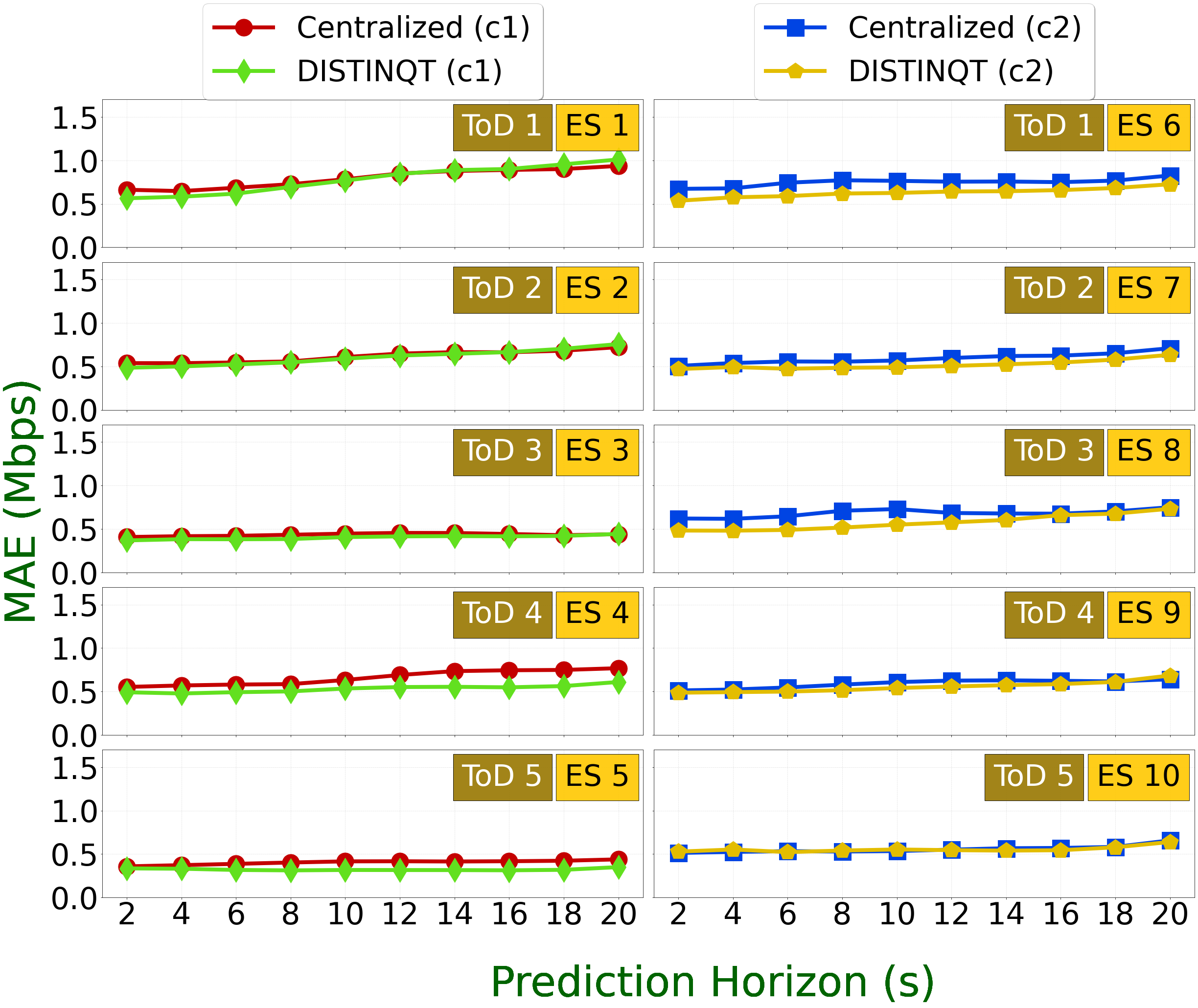
Figure 7: QoS prediction performance of DISTINQT and Centralized schemes over different prediction time horizons

	DISTINQT (c1)		Centralized (c1)			DISTINQT (c2)		Centralized (c2)
Avg. (Mbps) ($\pm$ STD)	Overall MAE	20th Second MAE	Overall MAE	20th Second MAE	Avg. (Mbps) ($\pm$ STD)	Overall MAE	20th Second MAE	Overall MAE	20th Second MAE
ToD 1, ES 1	0.7615 ($\pm$ 2.532)	1.0102 ($\pm$ 2.617)	0.7798 ($\pm$ 2.299)	0.9360 ($\pm$ 2.038)	ToD 1, ES 6	0.6173 ($\pm$ 2.079)	0.7253 ($\pm$ 1.916)	0.7348 ($\pm$ 2.357)	0.82257 ($\pm$ 2.042)
ToD 2, ES 2	0.5833 ($\pm$ 2.018)	0.7664 ($\pm$ 2.116)	0.6039 ($\pm$ 1.737)	0.7210 ($\pm$ 1.37)	ToD 2, ES 7	0.524 ($\pm$ 1.484)	0.6334 ($\pm$ 1.311)	0.5892 ($\pm$ 1.715)	0.7089 ($\pm$ 1.456)
ToD 3, ES 3	0.3968 ($\pm$ 1.086)	0.4425 ($\pm$ 0.745)	0.4284 ($\pm$ 1.099)	0.4398 ($\pm$ 0.538)	ToD 3, ES 8	0.5665 ($\pm$ 1.801)	0.7323 ($\pm$ 1.84)	0.6644 ($\pm$ 2.214)	0.7498 ($\pm$ 1.668)
ToD 4, ES 4	0.5187 ($\pm$ 1.245)	0.6093 ($\pm$ 0.917)	0.6496 ($\pm$ 1.692)	07679 ($\pm$ 1.18)	ToD 4, ES 9	0.5396 ($\pm$ 1.622)	0.6837 ($\pm$ 1.521)	0.578 ($\pm$ 1.802)	0.64 ($\pm$ 1.344)
ToD 5, ES 5	0.3183 ($\pm$ 0.78)	0.3497 ($\pm$ 0.363)	0.3989 ($\pm$ 1.051)	0.4387 ($\pm$ 0.569)	ToD 5, ES 10	0.5441 ($\pm$ 1.262)	0.6383 ($\pm$ 0.791)	0.5576 ($\pm$ 1.365)	0.6569 ($\pm$ 0.925)

TABLE VI: DISTINQT vs Centralized QoS prediction performance for 10 indicative and challenging evaluation scenarios

Fig. 6 presents the comparison between the groundtruth (actual values of uplink throughput) and the predicted output, for both QoS prediction approaches and for each of the 5 ToD-UEs. For presentation simplicity we have selected one indicative ES for each input feature configuration and for each ToD-UE. The timeline of each ES illustrates the predicted QoS value and corresponding groundtruth at intervals of 1 second ($t=1$ sec), specifically focusing on the 20th-second prediction timestep within the prediction horizon. From Fig. 6 it is evident that both approaches are able to capture the vast majority of the uplink throughput fluctuations for the different ToD-UEs in all evaluation scenarios.

Complementary to Fig. 6, Table VI and Fig. 7 indicate once again a statistically similar performance between our DISTINQT framework and the centralized approach in all evaluation scenarios. More specifically, Fig. 7 illustrates the performance of both approaches over different prediction horizons (in seconds). Intuitively, the further in time a prediction is made, the higher is the introduced MAE score and -as a result- the lower the model’s performance. DISTINQT in almost all evaluation scenarios and prediction horizons achieves a slightly better performance under both configurations c1 and c2, as it can also be inferred from the overall MAE score of Table VI.

In summary, our proposed DISTINQT framework can achieve and even surpass the performance of a high performing state-of-the-art LSTM-based centralized approach, considering different NETs, input feature configurations and prediction horizons. Evaluation results also showcase the contribution of the additional input features of the MEC Server NET to the overall performance of the DISTINQT.

V-B Baseline Comparisons

Apart from the comparison analysis between our DISTINQT framework and the centralized LSTM-based approach [51], this last round of evaluation results includes a comparison with six additional state-of-the-art centralized baseline solutions for different prediction time horizons and for all evaluation scenarios of the ToD-UEs. Specifically, these baseline solutions are the following:

• ARIMA: An Autoregressive integrated moving average (ARIMA) model, [52], estimating the uplink throughput solely based on the historical values of the uplink throughput.

• ARIMA-RF: A Random Forest (RF) Regressor, estimating the uplink throughput at a specific prediction timestep, exploiting ARIMA-based input estimates [10].

• RF Regressor: A standalone RF Regressor, estimating the uplink throughput over a prediction horizon, [53].

• k-NN Regressor, MLP & XGBoost: 3 different baseline solutions, namely a k-Nearest Neighbor (k-NN) Regressor, a Multi-Layer Perceptron (MLP) and an eXtreme Gradient Boosting (XGBoost), employed in the work [54] for QoS prediction.

Figs. 8, 9 and Table VII present the baseline comparison results. DISTINQT outperforms all baseline solutions in all selected prediction time horizons and under both input feature configurations, retaining a stable performance as the prediction time horizon increases. Table VII includes a detailed overview concerning the performance of all solutions for both input feature configurations. The table showcases the effectiveness of our approach by achieving an average performance improvement equal to 65% and 64% for the overall MAE score and 61.5% and 61.1% for the 20th second MAE under configurations c1 and c2, respectively.

Figure 8: QoS prediction performance between DISTINQT and six centralized state-of-the-art methods for c1

Figure 9: Qos prediction performance between DISTINQT and six centralized state-of-the-art methods for c2

	Configuration c1		Configuration c2
Avg. (Mbps) ($\pm$ STD)	Overall MAE	20th Second MAE	Overall MAE	20th Second MAE
DISTINQT	0.554 ($\pm$1.578)	0.6854 ($\pm$1.434)	0.529 ($\pm$1.574)	0.6388 ($\pm$1.325)
ARIMA	2.003 ($\pm$4.21)	3.4374 ($\pm$3.432)	2.003 ($\pm$4.21)	3.4374 ($\pm$3.432)
ARIMA-RF	2.3915 ($\pm$4.557)	3.6365 ($\pm$3.526)	2.2613 ($\pm$4.006)	3.3799 ($\pm$3.66)
kNN	1.4297 ($\pm$3.746)	1.3723 ($\pm$2.489)	1.3665 ($\pm$3.413)	1.3315 ($\pm$2.79)
RF	1.3249 ($\pm$2.791)	1.4869 ($\pm$1.539)	1.2371 ($\pm$2.653)	1.396 ($\pm$1.532)
XGBoost	1.6846 ($\pm$1.904)	1.6692 ($\pm$1.397)	1.5202 ($\pm$1.76)	1.5032 ($\pm$1.247)
MLP	1.2206 ($\pm$2.57)	1.255 ($\pm$1.231)	1.0638 ($\pm$2.466)	1.0753 ($\pm$1.257)

TABLE VII: QoS prediction performance comparison between DISTINQT and six baselines for c1 & c2

Concluding, this section highlights the effectiveness and validity of our DISTINQT framework by showcasing that a distributed approach for QoS prediction can successfully outperform six state-of-the-art centralized solutions.

VI Conclusions

This paper introduces and demonstrate the effectiveness of DISTINQT, a novel privacy-aware distributed learning framework for QoS prediction in the presence of heterogeneous data types and model architectures. DISTINQT is based on sequence-to-sequence autoencoders, distributing various NN-Encoders across the network and contributing to data privacy preservation. Our framework is evaluated in the Tele-Operated Driving use case, where evaluation results show that it can reach and even surpass the performance of its centralized counterpart. This is especially important for such safety critical use cases that require immediate and accurate decision making without compromising any sensitive information. Finally, DISTINQT achieves an average performance improvement of up to 65%, compared to six state-of-the-art centralized baseline solutions. Our future work will focus on finding a balance between the communication overhead that is introduced in the learning process and the robustness and generalization capabilities of the model.

References

- [1] W. Jiang, B. Han, M. A. Habibi, and H. D. Schotten, “The road towards 6g: A comprehensive survey,” IEEE Open Journal of the Communications Society, vol. 2, pp. 334–366, 2021.
- [2] M. Moussaoui, E. Bertin, and N. Crespi, “5g shortcomings and beyond-5g/6g requirements,” in 2022 1st International Conference on 6G Networking (6GNet), 2022, pp. 1–8.
- [3] one6G, “6g vertical use cases,” Tech. Rep., June 2022. [Online]. Available: https://one6g.org/download/2027/
- [4] 5GAA, “Making 5G Proactive and Predictive for the Automotive Industry,” White Paper, November 2019.
- [5] A. Kaloxylos, A. Gavras, D. Camps Mur, M. Ghoraishi, and H. Hrasnica, “Ai and ml – enablers for beyond 5g networks,” Dec. 2020. [Online]. Available: https://doi.org/10.5281/zenodo.4299895
- [6] R. Zhohov, A. Palaios, and P. Geuer, “One step further: Tunable and explainable throughput prediction based on large-scale commercial networks,” in 2021 IEEE 4th 5G World Forum (5GWF), 2021, pp. 430–435.
- [7] D. Minovski, N. Ogren, C. Ahlund, and K. Mitra, “Throughput prediction using machine learning in lte and 5g networks,” IEEE Transactions on Mobile Computing, pp. 1–1, 2021.
- [8] B. Sliwa, H. Schippers, and C. Wietfeld, “Machine learning-enabled data rate prediction for 5g nsa vehicle-to-cloud communications,” in 2021 IEEE 4th 5G World Forum (5GWF), 2021, pp. 299–304.
- [9] M. A. Gutierrez-Estevez, Z. Utkovski, A. Kousaridas, and C. Zhou, “A statistical learning framework for qos prediction in v2x,” in 2021 IEEE 4th 5G World Forum (5GWF), 2021, pp. 441–446.
- [10] A. Kousaridas, R. P. Manjunath, J. Perdomo, C. Zhou, E. Zielinski, S. Schmitz, and A. Pfadler, “Qos prediction for 5g connected and automated driving,” IEEE Communications Magazine, vol. 59, no. 9, pp. 58–64, 2021.
- [11] A. Palaios, C. Vielhaus, D. F. Külzer, P. Geuer, R. Sattiraju, J. Fink, M. Kasparick, C. Watermann, G. Fettweis, F. H. P. Fitzek, H. D. Schotten, and S. Stańczak, “Effect of spatial, temporal and network features on uplink and downlink throughput prediction,” in 2021 IEEE 4th 5G World Forum (5GWF), 2021, pp. 418–423.
- [12] one6G, “6g technology overview,” Tech. Rep. Third Edition, October 2023. [Online]. Available: https://one6g.org/download/3921/?tmstv=1697099550
- [13] O. Nassef, W. Sun, H. Purmehdi, M. Tatipamula, and T. Mahmoodi, “A survey: Distributed machine learning for 5g and beyond,” Computer Networks, vol. 207, p. 108820, 2022. [Online]. Available: https://www.sciencedirect.com/science/article/pii/S1389128622000421
- [14] 3GPP, “3rd Generation Partnership Project; Technical Specification Group Services and System Aspects; Study of Enablers for Network Automation for the 5G System (5GS); Phase 3 (Release 18),” Technical Report 3GPP TR 23.700-81, May 2022.
- [15] ETSI, “5G; Architecture enhancements for 5G System (5GS) to support network data analytics services (3GPP TS 23.288 version 17.4.0 Release 17),” Technical Specification ETSI TS 123 288 V17.4.0, May 2022.
- [16] 3GPP, “3rd Generation Partnership Project; Technical Specification Group Services and System Aspects; Study on AI/ML Model Transfer Phase 2 (Release 19),” Technical Report 3GPP TR 22.876 V19.1.0, September 2023.
- [17] Test case definition and test site description part 1. [Online]. Available: https://5gcroco.eu/images/templates/rsvario/images/5GCroCo_D2_1.pdf
- [18] Y. Zhang, X. Zhang, and X. Li, “Towards efficient and privacy-preserving service qos prediction with federated learning,” in Collaborative Computing: Networking, Applications and Worksharing, H. Gao, X. Wang, M. Iqbal, Y. Yin, J. Yin, and N. Gu, Eds. Cham: Springer International Publishing, 2021, pp. 37–57.
- [19] J. Xu, J. Lin, Y. Li, and Z. Xu, “Multifed: A fast converging federated learning framework for services qos prediction via cloud–edge collaboration mechanism,” Knowledge-Based Systems, vol. 268, p. 110463, 2023. [Online]. Available: https://www.sciencedirect.com/science/article/pii/S0950705123002137
- [20] X. Li, S. Li, Y. Li, Y. Zhou, C. Chen, and Z. Zheng, “A personalized federated tensor factorization framework for distributed iot services qos prediction from heterogeneous data,” IEEE Internet of Things Journal, vol. 9, no. 24, pp. 25 460–25 473, 2022.
- [21] I. Sutskever, O. Vinyals, and Q. V. Le, “Sequence to sequence learning with neural networks,” in Advances in Neural Information Processing Systems, Z. Ghahramani, M. Welling, C. Cortes, N. Lawrence, and K. Weinberger, Eds., vol. 27. Curran Associates, Inc., 2014.
- [22] L. Magoula, N. Koursioumpas, S. Barmpounakis, P. Kontopoulos, M. A. Gutierrez-Estevez, R. Khalili, and A. Kousaridas, “A deep learning approach for distributed qos prediction in beyond 5g networks,” in 2022 IEEE 33rd Annual International Symposium on Personal, Indoor and Mobile Radio Communications (PIMRC), 2022, pp. 1407–1412.
- [23] Q. Yang, Y. Liu, T. Chen, and Y. Tong, “Federated machine learning: Concept and applications,” vol. 10, no. 2, jan 2019. [Online]. Available: https://doi.org/10.1145/3298981
- [24] F. Z. Errounda and Y. Liu, “A mobility forecasting framework with vertical federated learning,” in 2022 IEEE 46th Annual Computers, Software, and Applications Conference (COMPSAC), 2022, pp. 301–310.
- [25] J. Ryu, D. Won, and Y. Lee, “A study of split learning model,” in 2022 16th International Conference on Ubiquitous Information Management and Communication (IMCOM), 2022, pp. 1–4.
- [26] J. Jeon and J. Kim, “Privacy-sensitive parallel split learning,” in 2020 International Conference on Information Networking (ICOIN), 2020, pp. 7–9.
- [27] J. Kim, S. Park, S. Jung, and S. Yoo, “Spatio-temporal split learning,” 2021 51st Annual IEEE/IFIP International Conference on Dependable Systems and Networks - Supplemental Volume (DSN-S), pp. 11–12, 2021.
- [28] Q. Sun, J. Xu, X. Ma, A. Zhou, C.-H. Hsu, and S. Wang, “Edge-enabled distributed deep learning for 5g privacy protection,” IEEE Network, vol. 35, no. 4, pp. 213–219, 2021.
- [29] D. Saguil and A. Azim, “A layer-partitioning approach for faster execution of neural network-based embedded applications in edge networks,” IEEE Access, vol. 8, pp. 59 456–59 469, 2020.
- [30] T. Mohammed, C. Joe-Wong, R. Babbar, and M. D. Francesco, “Distributed inference acceleration with adaptive dnn partitioning and offloading,” in IEEE INFOCOM 2020 - IEEE Conference on Computer Communications, 2020, pp. 854–863.
- [31] Z. Xu, L. Zhao, W. Liang, O. F. Rana, P. Zhou, Q. Xia, W. Xu, and G. Wu, “Energy-aware inference offloading for dnn-driven applications in mobile edge clouds,” IEEE Transactions on Parallel and Distributed Systems, vol. 32, no. 4, pp. 799–814, 2021.
- [32] L. Zeng, X. Chen, Z. Zhou, L. Yang, and J. Zhang, “Coedge: Cooperative dnn inference with adaptive workload partitioning over heterogeneous edge devices,” IEEE/ACM Transactions on Networking, vol. 29, no. 2, pp. 595–608, 2021.
- [33] J. Du, X. Zhu, M. Shen, Y. Du, Y. Lu, N. Xiao, and X. Liao, “Model parallelism optimization for distributed inference via decoupled cnn structure,” IEEE Transactions on Parallel and Distributed Systems, vol. 32, no. 7, pp. 1665–1676, 2021.
- [34] Z. Hu, A. B. Tarakji, V. Raheja, C. Phillips, T. Wang, and I. Mohomed, “Deephome: Distributed inference with heterogeneous devices in the edge,” in The 3rd International Workshop on Deep Learning for Mobile Systems and Applications, ser. EMDL ’19. New York, NY, USA: Association for Computing Machinery, 2019, p. 13–18. [Online]. Available: https://doi.org/10.1145/3325413.3329787
- [35] J. Zhai, S. Zhang, J. Chen, and Q. He, “Autoencoder and its various variants,” in 2018 IEEE International Conference on Systems, Man, and Cybernetics (SMC), 2018, pp. 415–419.
- [36] N. Phan, Y. Wang, X. Wu, and D. Dou, “Differential privacy preservation for deep auto-encoders: An application of human behavior prediction,” in Proceedings of the Thirtieth AAAI Conference on Artificial Intelligence, ser. AAAI’16. AAAI Press, 2016, p. 1309–1316.
- [37] H. C. Tanuwidjaja, R. Choi, S. Baek, and K. Kim, “Privacy-preserving deep learning on machine learning as a service—a comprehensive survey,” IEEE Access, vol. 8, pp. 167 425–167 447, 2020.
- [38] H. Ning, Ed., Cyberspace Data and Intelligence, and Cyber-Living, Syndrome, and Health. Springer, Singapore, 2019.
- [39] R. M. Alguliyev, R. M. Aliguliyev, and F. J. Abdullayeva, “Privacy-preserving deep learning algorithm for big personal data analysis,” Journal of Industrial Information Integration, vol. 15, pp. 1–14, 2019. [Online]. Available: https://www.sciencedirect.com/science/article/pii/S2452414X18301456
- [40] K. Bayoudh, R. Knani, F. Hamdaoui, and A. Mtibaa, “A survey on deep multimodal learning for computer vision: advances, trends, applications, and datasets,” The Visual Computer, vol. 38, no. 8, pp. 2939–2970, Aug 2022. [Online]. Available: https://doi.org/10.1007/s00371-021-02166-7
- [41] I. Goodfellow, Y. Bengio, and A. Courville, Deep Learning. MIT Press, 2016, http://www.deeplearningbook.org.
- [42] “Deep neural networks compression: A comparative survey and choice recommendations,” Neurocomputing, vol. 520, pp. 152–170, 2023.
- [43] 5GAA, “C-V2X Use Cases, Methodology, Examples and Service Level Requirements,” White Paper, July 2019.
- [44] Official ns-3 website. [Online]. Available: https://www.nsnam.org/
- [45] 3rd Generation Partnership Project (3GPP), “Study on Scenarios and Requirements for Next Generation Access Technologies (Rel. 16),” Technical Report (TR) 38.913, July 2020.
- [46] 3rd Generation Partnership Project (3GPP), “Study on evaluation methodology of new Vehicle-to-Everything (V2X) use cases for LTE and NR (Rel. 15),” Technical Report (TR) 37.885, June 2019.
- [47] G. A. A. (5GAA), “Tele-operated Driving Use Cases, System Architecture and Business Considerations,” White Paper, December 2021.
- [48] Simulation of urban mobility. [Online]. Available: https://eclipse.dev/sumo/
- [49] L. Prechelt, Early Stopping - But When? Berlin, Heidelberg: Springer Berlin Heidelberg, 1998, pp. 55–69. [Online]. Available: https://doi.org/10.1007/3-540-49430-8_3
- [50] C. Sammut and G. I. Webb, Eds., Mean Absolute Error. Boston, MA: Springer US, 2010, pp. 652–652.
- [51] S. Barmpounakis, L. Magoula, N. Koursioumpas, R. Khalili, J. M. Perdomo, and R. P. Manjunath, “Lstm-based qos prediction for 5g-enabled connected and automated mobility applications,” in 2021 IEEE 4th 5G World Forum (5GWF), 2021, pp. 436–440.
- [52] R. Madan and P. S. Mangipudi, “Predicting computer network traffic: A time series forecasting approach using dwt, arima and rnn,” in 2018 Eleventh International Conference on Contemporary Computing (IC3), 2018, pp. 1–5.
- [53] A. Palaios, C. Vielhaus, D. F. Külzer, P. Geuer, R. Sattiraju, J. Fink, M. Kasparick, C. Watermann, G. Fettweis, F. H. P. Fitzek, H. D. Schotten, and S. Stańczak, “Effect of spatial, temporal and network features on uplink and downlink throughput prediction,” in 2021 IEEE 4th 5G World Forum (5GWF), 2021, pp. 418–423.
- [54] S. Barmpounakis, N. Maroulis, N. Koursioumpas, A. Kousaridas, A. Kalamari, P. Kontopoulos, and N. Alonistioti, “Ai-driven, qos prediction for v2x communications in beyond 5g systems,” Computer Networks, vol. 217, p. 109341, 2022. [Online]. Available: https://www.sciencedirect.com/science/article/pii/S1389128622003759