Local gluing

Abstract

In the local gluing one glues local neighborhoods around the critical point of the stable and unstable manifolds to gradient flow lines defined on a finite time interval $[-T,T]$ for large $T$. If the Riemannian metric around the critical point is locally Euclidean, the local gluing map can be written down explicitly. In the non-Euclidean case the construction of the local gluing map requires an intricate version of the implicit function theorem.

In this paper we explain a functional analytic approach how the local gluing map can be defined. For that we are working on infinite dimensional path spaces and also interpret stable and unstable manifolds as submanifolds of path spaces. The advantage of this approach is that similar functional analytical techniques can as well be generalized to infinite dimensional versions of Morse theory, for example Floer theory.

A crucial ingredient is the Newton-Picard map. We work out an abstract version of it which does not involve troublesome quadratic estimates.

1 Introduction and main results

1.1 Local gluing map for the Euclidean metric

Consider a diagonal matrix with monotone decreasing diagonal entries

$$A={\rm diag}(a_{1},\dots,a_{n}),\qquad a_{1}\geq\dots\geq a_{n-k}>0>a_{n-k+1}\geq\dots\geq a_{n}.$$

Consider the smooth function given by the euclidean inner product

$$f\colon{\mathbb{R}}^{n}\to{\mathbb{R}},\quad z\mapsto\tfrac{1}{2}\left\langle z,Az\right\rangle.$$ (1.1)

This function is Morse and has a unique critical point at the origin of Morse index $k$. The gradient of $f$ for the standard metric on ${\mathbb{R}}^{n}$ is $\nabla\kern-2.15277ptf(z)=Az$. Hence the downward gradient flow for time $s$ is given by

$$\varphi^{-\nabla\kern-1.50694ptf}_{s}(z)=e^{-sA}z=\left(e^{-sa_{1}}z_{1},\dots,e^{-sa_{n}}z_{n}\right).$$

The stable and the unstable manifold of the origin are given by the sets

$$W^{\rm s}={\mathbb{R}}^{n-k}\times\{0\},\qquad W^{\rm u}=\{0\}\times{\mathbb{R}}^{k}.$$

Each point $z_{0}=(x_{0},0)\in{\mathbb{R}}^{n-k}\times\{0\}$ determines an element $s\mapsto w_{+}(s):=e^{-sA}z_{0}$ in the function space $W^{1,2}([0,\infty),{\mathbb{R}}^{n})$. Each point $z_{0}=(0,y_{0})\in\{0\}\times{\mathbb{R}}^{k}$ determines an element $s\mapsto w_{-}(s):=e^{-sA}z_{0}$ in the function space $W^{1,2}((-\infty,0],{\mathbb{R}}^{n})$.

In our functional analytic approach to local gluing it is more convenient for us to think of the stable and the unstable manifold as function space subsets

$${\mathcal{W}}^{\rm s}\subset W^{1,2}([0,\infty),{\mathbb{R}}^{n}),\qquad{\mathcal{W}}^{\rm u}\subset W^{1,2}((-\infty,0],{\mathbb{R}}^{n}).$$

A further advantage of this point of view is that many techniques discussed in this article can be generalized from ${\mathbb{R}}^{n}$ to the Hardy approach of gluing in the infinite dimensional case of Floer homology [Sim14].

With the interpretation of stable and unstable manifolds as function spaces we can easily recover the traditional interpretation as subsets of ${\mathbb{R}}^{n}$ using the evaluation maps

$${\rm ev}_{+}\colon{\mathcal{W}}^{\rm s}\to{\mathbb{R}}^{n-k}\times\{0\},\quad w_{+}\mapsto w_{+}(0)$$

and

$${\rm ev}_{-}\colon{\mathcal{W}}^{\rm u}\to\{0\}\times{\mathbb{R}}^{k},\quad w_{-}\mapsto w_{-}(0).$$

Given $T>0$, let ${\mathcal{M}}_{T}\subset W^{1,2}([-T,T],{\mathbb{R}}^{n})$ be the subset of all finite time gradient flow lines $w\colon[-T,T]\to{\mathbb{R}}^{n}$. Note that since in the euclidean case the gradient flow is linear and a gradient flow line is uniquely determined by its initial condition, the space ${\mathcal{M}}_{T}$ is an $n$-dimensional linear subspace of the infinite dimensional function space $W^{1,2}([-T,T],{\mathbb{R}}^{n})$.

In the euclidean case, that is ${\mathbb{R}}^{n}$ endowed with the standard metric, there are natural linear isomorphisms

$$\Gamma_{T}\colon{\mathcal{W}}^{\rm s}\times{\mathcal{W}}^{\rm u}\to{\mathcal{M}}_{T}$$

called the local gluing maps and given at each time $s\in[-T,T]$ by

$$\Gamma_{T}(w_{+},w_{-})(s)=e^{-(s+T)A}w_{+}(0)+e^{(T-s)A}w_{-}(0).$$ (1.2)

Consider the evaluation map defined by

$${\rm ev}_{T}\colon W^{1,2}([-T,T],{\mathbb{R}}^{n})\to{\mathbb{R}}^{n}\times{\mathbb{R}}^{n},\quad w\mapsto\left(w(-T),w(T)\right).$$

The composition of the local gluing maps $\Gamma_{T}$ with the evaluation map ${\rm ev}_{T}$ is a linear map, namely

$${\rm ev}_{T}\circ\Gamma_{T}(w_{+},w_{-})=\left(w_{+}(0)+e^{2TA}w_{-}(0),w_{-}(0)+e^{-2TA}w_{+}(0)\right).$$

Since $w_{-}$ is in the unstable manifold and $w_{+}$ in the stable, both limits are zero

$$\lim_{T\to\infty}e^{2TA}w_{-}(0)=0,\qquad\lim_{T\to\infty}e^{-2TA}w_{+}(0)=0.$$

Therefore it holds that $\lim_{T\to\infty}{\rm ev}_{T}\circ\Gamma_{T}={\rm ev}$ where

$${\rm ev}=({\rm ev}_{+},{\rm ev}_{-})\colon{\mathcal{W}}^{\rm s}\times{\mathcal{W}}^{\rm u}\to{\mathbb{R}}^{n}\times{\mathbb{R}}^{n},\quad(w_{+},w_{-})\mapsto\left(w_{+}(0),w_{-}(0)\right).$$

1.2 Local gluing map for a general Riemannian metric

Given a general Morse function $f$ on a finite dimensional manifold, by the Morse Lemma one can always find locally around each critical point coordinates such that $f$ has the form (1.1) after subtracting the critical value. In fact, it is even possible, after some additional scaling, to assume that all diagonal entries of the matrix $A$ are either $1$ or $-1$. In infinite dimension this is usually not possible and therefore we don’t use this fact.
Unfortunately, even in finite dimension, it is in general not possible to assume that in Morse coordinates the Riemannian metric is standard as well. Indeed curvature is an obstruction.

In this article we explain, based on a special version of Newton-Picard iteration, a functional analytic construction for local gluing maps $\gamma_{T}$ in the curved case. In sharp contrast to the Euclidean version $\Gamma_{T}$, the local gluing maps $\gamma_{T}$ are in general not linear. However, still some of the major properties of the local gluing maps $\Gamma_{T}$ in the flat case are preserved in the general case. More precisely, we have the following theorem.

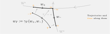
Figure 1: Convergence of local gluing ${\rm ev}_{T}\circ\gamma_{T}(w_{+},w_{-})\stackrel{{\scriptstyle T\to\infty}}{{\longrightarrow}}{\rm ev}(w_{+},w_{-})$

Theorem A (Local gluing).

There are open neighborhoods ${\mathcal{U}}_{+}$ and ${\mathcal{U}}_{-}$ of the origin in the stable and unstable manifold and gluing maps $\gamma_{T}\colon{\mathcal{U}}_{+}\times{\mathcal{U}}_{-}\to{\mathcal{M}}_{T}$ for $T\geq T_{0}$, where ${\mathcal{M}}_{T}$ is the space of downward gradient flow lines on the finite time interval $[-T,T]$, which have the following properties.

• For every $T\geq T_{0}$ the gluing map $\gamma_{T}$ is a diffeomorphism onto its image

• In the limit $T\to\infty$ in the $C^{\infty}$ topology the diagram

  (1.3)

  commutes, as illustrated by Figure 1, where $ev$ and ${\rm ev}_{T}$ are the evaluation maps at the end points.

Remark 1.1.

Our construction of local gluing maps $\gamma_{T}$ has the following additional properties.

1. In the euclidean case it holds that $\gamma_{T}=\Gamma_{T}$.

2. In the general Riemannian case this still continues to hold for the differential of $\gamma_{T}$ at the origin, in symbols $d\gamma_{T}(0_{+},0_{-})=\Gamma_{T}$.

3. In particular, at the infinitesimal level, our construction is independent of any choices like the one of a cutoff function used to construct a pre-gluing map; see (2.11). The construction of the gluing map depends on the choice of a complement of the kernel ${\mathbb{E}}_{T}$ of the linearized gradient flow equation $D_{T}\colon{\mathbb{W}}_{T}\to{\mathbb{V}}_{T}$; see (4.39). There are different choices for such a complement. Possible choices are to take the complement orthogonal with respect to either the $L^{2}$ or the $W^{1,2}$ metric. We make a different choice, so that our complement ${\mathbb{K}}_{T}$ is not necessarily orthogonal, but instead has the property that the infinitesimal gluing map, see (3.26), does not depend on the choice of the cutoff function.

4. Furthermore, our construction uses a version of the Newton-Picard map which does not need quadratic estimates. We discuss properties of the Newton-Picard map and its derivatives in Appendix B.

   The results in Appendix B are quite general, so that they should also be applicable to the infinite dimensional version of the local gluing discussed in this article. Namely, the general Hardy approach to gluing, as discussed in the special case of Lagrangian Floer homology by Tatjana Simčević [Sim14].

We expect that the local gluing theorems will be useful for the construction of flow category theories [CJS95] by endowing, for Morse-Smale metrics, the moduli (solution) spaces of broken gradient flow lines with the structure of a manifold with boundary and corners [Qin18, Weh12].

1.3 Setup – path spaces and sections

Let $f\colon{\mathbb{R}}^{n}\to{\mathbb{R}}$ be a smooth function such that the origin $\mathrm{𝟎}$ is a Morse critical point of Morse index $k$. Suppose $g$ is a Riemannian metric on ${\mathbb{R}}^{n}$ which is standard at $\mathrm{𝟎}$, notation $g_{0}$. Let $\mathrm{Hess}_{0}f$ be the Hessian bilinear form of $f$ at $\mathrm{𝟎}$. The Hessian linear operator $A\colon{\mathbb{R}}^{n}\to{\mathbb{R}}^{n}$ color=yellow!40]$A$ is just the Hesse MATRIX since $g_{0}$ is standard of $f$ at $\mathrm{𝟎}$ is defined with the help of the metric $g_{0}$ by the formula $\mathrm{Hess}_{0}f(z_{1},z_{2})=g_{0}(z_{1},Az_{2})$ for every $z_{1},z_{2}\in{\mathbb{R}}^{n}$. After a linear change of coordinates we can assume that $A$ is a diagonal matrix with monotone decreasing diagonal entries

$$A={\rm diag}(a_{1},\dots,a_{n}),\qquad a_{1}\geq\dots\geq a_{n-k}>0>a_{n-k+1}\geq\dots\geq a_{n}.$$ (1.4)

Consider the $g_{0}$-orthogonal splitting

$${\mathbb{R}}^{n}={\mathbb{R}}^{n-k}\times{\mathbb{R}}^{k}\stackrel{{\scriptstyle p_{-}}}{{\longrightarrow}}{\mathbb{R}}^{k},\quad(x,y)\mapsto y,\qquad p_{+}(x,y):=x.$$ (1.5)

Then the Hessian at $\mathrm{𝟎}$ is positive definite on $E^{+}={\mathbb{R}}^{n-k}\times\{0\}$ and negative definite on $E^{-}=\{0\}\times{\mathbb{R}}^{k}$. The Hessian operator at $\mathrm{𝟎}$ is of the form

$$A=\begin{pmatrix}A_{+}&0\\ 0&-A_{-}\end{pmatrix}$$ (1.6)

where $A_{+}={\rm diag}(a_{1},\dots,a_{n-k})$ and $A_{-}={\rm diag}(-a_{n-k+1},\dots,-a_{n})$ are positive definite diagonal matrices. The spectral gap $\sigma=\sigma(A)>0$ is the smallest distance of an eigenvalue to the origin, in symbols

$$\sigma=\sigma(A):=\min_{1\leq\ell\leq n}\mathopen{|}a_{\ell}\mathclose{|}.$$ (1.7)

Abbreviate ${\mathbb{R}}_{+}=(0,\infty)$. For $T>0$ consider the Sobolev spaces

$${\mathbb{W}}_{+}=W^{1,2}([0,\infty),{\mathbb{R}}^{n}),\;{\mathbb{W}}_{-}=W^{1,2}((-\infty,0],{\mathbb{R}}^{n}),\;{\mathbb{W}}_{T}=W^{1,2}([-T,T],{\mathbb{R}}^{n}),$$

$${\mathbb{V}}_{+}=L^{2}([0,\infty),{\mathbb{R}}^{n}),\quad{\mathbb{V}}_{-}=L^{2}((-\infty,0],{\mathbb{R}}^{n}),\quad{\mathbb{V}}_{T}=L^{2}([-T,T],{\mathbb{R}}^{n}).$$

Definition 1.2 (Constant maps to the critical point).

Let $0_{+}\in{\mathbb{W}}_{+}$ and $0_{-}\in{\mathbb{W}}_{-}$, and $0_{T}\in{\mathbb{W}}_{T}$, be the constant maps to the critical point, in symbols

$$0_{+}\colon[0,\infty)\to{\mathbb{R}}^{n},\quad s\mapsto 0,\qquad 0_{-}\colon(\infty,0]\to{\mathbb{R}}^{n},\mapsto s\mapsto 0.$$

Let $0_{T}\in{\mathbb{W}}_{T}$ be the constant map $[-T,T]\to{\mathbb{R}}^{n}$, $s\mapsto 0$, to the critical point.

For $i\in\{+,-\}\cup{\mathbb{R}}_{+}$ consider the map defined by

$${\mathcal{F}}_{i}\colon{\mathbb{W}}_{i}\to{\mathbb{V}}_{i},\quad w\mapsto{\partial}_{s}w+\nabla\kern-2.15277ptf(w).$$

The zero sets of these maps are, respectively, the stable and the unstable manifold, and the set of gradient flow lines along the interval $[-T,T]$, in symbols

$${\mathcal{W}}^{\rm s}:={{\mathcal{F}}_{+}}^{-1}(0_{+})\subset{\mathbb{W}}_{+},\qquad{\mathcal{W}}^{\rm u}:={{\mathcal{F}}_{-}}^{-1}(0_{-})\subset{\mathbb{W}}_{-},$$

and the solution space

$${\mathcal{M}}_{T}:={{\mathcal{F}}_{T}}^{-1}(0_{T})=\{w\colon[-T,T]\stackrel{{\scriptstyle W^{1,2}}}{{\to}}{\mathbb{R}}^{n}\mid{\partial}_{s}w+\nabla\kern-2.15277ptf(w)=0\}\subset{\mathbb{W}}_{T}.$$

The elements of the tangent spaces at the critical point

$$\xi\in{\mathbb{E}}^{+}:=T_{0_{+}}{\mathcal{W}}^{\rm s},\qquad\eta\in{\mathbb{E}}^{-}:=T_{0_{-}}{\mathcal{W}}^{\rm u},\qquad\zeta\in{\mathbb{E}}_{T}:=T_{0_{T}}{\mathcal{M}}_{T},$$

are characterized by the linear autonomous ODEs (2.15) or, equivalently, by forward (backward) exponential decay (2.17) of $\xi=(\xi^{+},0)$ (of $\eta=(0,\eta^{-})$).

Notation. The color=yellow!40] Spaces
$E^{+}$ linear point space
$\mathbb{E}^{+}$ linear map space
${\mathcal{E}}^{+}$ manifold of maps euclidean norm of $v\in{\mathbb{R}}^{\ell}$, $\ell\in{\mathbb{N}}$, is denoted by $\mathopen{|}v\mathclose{|}$.

1.4 Idea of proof

We construct the desired gluing map as a family of diffeomorphisms onto their images, one diffeomorphism for each $T\geq T_{0}$ given by composing two maps

$$\gamma_{T}\colon{\mathcal{W}}^{\rm s}\times{\mathcal{W}}^{\rm u}\supset{\mathcal{U}}_{+}\times{\mathcal{U}}_{-}\stackrel{{\scriptstyle\wp_{T}}}{{\longrightarrow}}{\mathbb{W}}_{T}\stackrel{{\scriptstyle{\mathcal{N}}_{T}}}{{\longrightarrow}}{\mathcal{M}}_{T}.$$ (1.8)

Here $T_{0}\geq 3$ is a constant and ${\mathcal{U}}_{+}\subset{\mathcal{W}}^{\rm s}$ and ${\mathcal{U}}_{-}\subset{\mathcal{W}}^{\rm u}$ are open neighborhoods of $0_{+}$ and $0_{-}$, respectively, sufficiently small so that the image $\wp_{T}({\mathcal{U}}_{+}\times{\mathcal{U}}_{-})$ of the pre-gluing map $\wp_{T}$ lies in the domain of the Newton-Picard map ${\mathcal{N}}_{T}$.

Newton-Picard. The Newton-Picard map on $X={\mathbb{W}}_{T}$ associates to an approximate zero of a map, here ${\mathcal{F}}_{T}$, a true zero nearby. More precisely, after choosing a suitable initial point $x_{0}$, here $0_{T}$, there are three ingredients needed:

1) an approximate zero $x_{1}$ of ${\mathcal{F}}_{T}$;
2) a uniformly bounded right inverse $Q_{T}$ of $D_{T}:=d{\mathcal{F}}_{T}(0_{T})\colon{\mathbb{W}}_{T}\to{\mathbb{V}}_{T}$;
3) a slowly varying operator difference $d{\mathcal{F}}_{T}(\cdot)-D_{T}$ near the initial point.

The facts that ${\mathcal{F}}_{T}(0_{T})=0$ and that $D_{T}$ is surjective suggest to choose as initial point $x_{0}:=0_{T}$. 1) To provide an approximate zero of ${\mathcal{F}}_{T}$ will be the task of the pre-gluing map as described further below. 2) Right inverses of the linear operator $D_{T}\colon{\mathbb{W}}_{T}\to{\mathbb{V}}_{T}$ correspond to the topological complements of $\ker D_{T}$. A natural choice would be the orthogonal complement, but we shall choose another complement, notation ${\mathbb{K}}_{T}$, which represents the impossible paths for a downward gradient and makes the infinitesimal gluing map $\Gamma_{T}=d\gamma_{T}(0_{+},0_{-})$ independent of the choice of cutoff function used to define the pre-gluing map. The corresponding right inverse $Q_{T}$ indeed admits a uniform bound $c$. 3) The operator difference $d{\mathcal{F}}_{T}(\cdot)-D_{T}$ is usually controlled by calculating troublesome quadratic estimates. In Appendix B.1 we prove continuous differentiability of a version of the Newton-Picard map which does not require quadratic estimates.

Remark 1.3 (Higher smoothness of Newton-Picard map).

To obtain higher smoothness we use, roughly speaking, the fact that the supremum of the operator norm $\mathopen{\|}d{\mathcal{F}}_{T}(\cdot)-D_{T}\mathclose{\|}$ along smaller and smaller balls about the initial point $x_{0}$ admits bounds closer and closer to zero. Indeed there is a monotonically decreasing function $\delta\colon[2,\infty)\to(0,\infty)$, independent of $T$, such that along the $\delta(\mu)$-ball about $x_{0}$ the map $\mathopen{\|}d{\mathcal{F}}_{T}(\cdot)-D_{T}\mathclose{\|}$ is bounded by $1/\mu c$. See Corollary 4.5 for the case of ${\mathcal{F}}_{T}$ and Remark B.8 for the abstract theory.

For iteration arguments, such as to prove higher smoothness, tangent maps are much more suitable than differentials. Thus we prove in Appendix B.2 an estimate for the tangent map difference $T{\mathcal{N}}-{\rm Id}$ and we show that $T{\mathcal{N}}^{F}={\mathcal{N}}^{TF}$, roughly speaking, where ${\mathcal{N}}^{F}$ is the Newton-Picard map for a map $F$.

Pre-gluing – approximate zero. Given a real $T\geq 3$, called gluing parameter, Floer’s gluing construction associates to a pair $(w_{+},w_{-})\in{\mathcal{W}}^{\rm s}\times{\mathcal{W}}^{\rm u}$ of an $(\text{incoming},\text{outgoing})$ flow trajectory the pre-glued path $w_{T}\colon[-T,T]\to{\mathbb{R}}^{m}$ defined as follows. One decomposes the time interval $[-T,T]$ into five subintervals. Along $[-T,-3]$ follow the backward shifted forward flow trajectory $w_{+}(T+\cdot)$, then along $[-3,-1]$ interpolate with the help of a cutoff function to the constant flow trajectory $s\mapsto 0$ sitting at the critical point at which $w_{T}$ then rests along time $[-1,1]$. Next along time $[1,3]$ interpolate from the constant map $s\mapsto 0$ to the forward shifted backward flow trajectory $w_{-}(-T+\cdot)$ which then represents $w_{T}$ along the final time interval $[3,T]$.

The behavior of the pre-glued path $w_{T}\colon[-T,T]\to{\mathbb{R}}^{n}$ along the five time intervals is detailed by formula (2.12) and illustrated by Figure 2. Observe that $w_{T}$ takes on the boundary of its domain $[-T,T]$ values that do not depend on $T$, namely $w_{+}(0)$ and $w_{-}(0)$. Most importantly, the pre-glued path satisfies the gradient equation except, possibly, along the subinterval $[-3,-1]$ (and $[1,3]$) of $[-T,T]$ along which it coincides, up to a cutoff function factor, with the forward flow trajectory $w_{+}$ along $[T-3,T-1]$. But $w_{+}|_{[T-3,T-1]}$ is very close to the critical point for large $T$. Consequently uniform exponential decay of ${\partial}_{s}w_{+}$ takes care of the $L^{2}$ norm of ${\mathcal{F}}_{T}(w_{T})={\partial}_{s}w_{T}+\nabla\kern-2.15277ptf(w_{T})$ along $[-3,-1]$; same along $[1,3]$ where $w_{-}$ appears. With this understood it follows that $w_{T}$ is an approximate zero of ${\mathcal{F}}_{T}$ in the sense that

$$\mathopen{\|}{\mathcal{F}}_{T}(w_{T})\mathclose{\|}_{{\mathcal{V}}_{T}}\leq Ce^{-{\varepsilon}T}$$ (1.9)

whenever $T\geq 3$. The constant $C$ serves all elements $w_{\pm}$ of any chosen pair of compact neighborhoods $K_{\pm}$ of $0_{\pm}$ in the stable/unstable manifold.

Gluing – smooth convergence. With Newton-Picard and pre-gluing in place the gluing map $\gamma_{T}$, given by composition (1.8), is well defined. Appendix A revisits the proof of the usual IFT explained in [MS04, App. A.3] to extract a quantitative version. It is applied in Section 5.1 to prove that $\gamma_{T}$ is a diffeomorphism onto its image along a sufficiently small domain, uniformly in $T$.

In the limit $T\to\infty$ the diagram (1.3) commutes even after application of the $m$-fold tangent functor $T^{m}$. The proof uses techniques described by Remark 1.3 and is carried out in Section 5.2.

Outline of article

Section 2 “Pre-gluing map ${\mathcal{P}}_{T}$ and its restriction $\wp_{T}$” introduces for each parameter value $T\geq 3$ the pre-gluing map as the linear map ${\mathcal{P}}_{T}\colon{\mathbb{W}}_{+}\times{\mathbb{W}}_{-}\to{\mathbb{W}}_{T}$ defined by (2.11), equivalently by (2.12), and illustrated by Figure 2.

For $0_{+}\in{\mathcal{W}}^{\rm s}$ and $0_{-}\in{\mathcal{W}}^{\rm u}$ the pre-glued path is a true zero, more precisely ${\mathcal{P}}_{T}(0_{+},0_{-})=0_{T}\in{\mathcal{F}}_{T}^{-1}(0)\subset{\mathbb{W}}_{T}$. This motivates the expectation that pre-gluing pairs near $(0_{+},0_{-})\in{\mathcal{W}}^{\rm s}\times{\mathcal{W}}^{\rm u}$ should produce approximate zeroes. Thus we consider the restriction of the pre-gluing map ${\mathcal{P}}_{T}$, notation

$$\wp_{T}:={\mathcal{P}}_{T}|_{{\mathcal{W}}^{\rm s}\times{\mathcal{W}}^{\rm u}}\colon{\mathcal{W}}^{\rm s}\times{\mathcal{W}}^{\rm u}\to{\mathbb{W}}_{T}.$$ (1.10)

This map is smooth by linearity of ${\mathcal{P}}_{T}$. Whereas the elements of the tangent spaces to ${\mathcal{W}}^{\rm s}$, ${\mathcal{W}}^{\rm u}$, and ${\mathcal{M}}_{T}$ at the origins $0_{+}$, $0_{-}$, and $0_{T}$ (notation ${\mathbb{E}}^{\pm}$ and ${\mathbb{E}}_{T}$) are the solutions of autonomous linear ODEs (2.15), at general points $w_{+}$, $w_{-}$, and $w_{T}$ the characterizing linear ODE’s (2.18) are non-autonomous.

The linear identifications $\theta_{w_{\pm}}\colon T_{w_{\pm}}{\mathcal{W}}^{\rm s/u}\to{\mathbb{E}}^{\pm}$, defined via asymptotic limits, are used to prove Theorem 5.3 (gluing map $\gamma_{T}$ is diffeomorphism onto its image).

Section 3 “Infinitesimal gluing” consists of two subsections. Subsection 3.1 introduces a complement ${\mathbb{K}}_{T}$ of the $n$-dimensional subspace ${\mathbb{E}}_{T}:=T_{0_{T}}{\mathcal{M}}_{T}$ of ${\mathbb{W}}_{T}$ and the corresponding projection $P_{{\mathbb{E}}_{T},{\mathbb{K}}_{T}}$ onto ${\mathbb{E}}_{T}$ along ${\mathbb{K}}_{T}$, notation

$$\Pi_{T}:=P_{{\mathbb{E}}_{T},{\mathbb{K}}_{T}}\colon{\mathbb{W}}_{T}={\mathbb{K}}_{T}\oplus{\mathbb{E}}_{T}\to{\mathbb{E}}_{T}.$$

Lemma 3.3 provides a formula for $\Pi_{T}$ and asserts that the operator norm of $\Pi_{T}\colon{\mathbb{W}}_{T}\to{\mathbb{W}}_{T}$ is bounded by a constant $d=d(a_{1},a_{n})$, depending on the eigenvalues $a_{1}$ and $a_{n}$ of the Hessian $A$ in (1.4), but independent of $T\geq 1$. To prove this we establish the uniform-in-$T$ Sobolev estimate $\mathopen{\|}v\mathclose{\|}_{L^{\infty}[-T,T]}\leq 2\mathopen{\|}v\mathclose{\|}_{W^{1,2}[-T,T]}$. Later on the estimate also enters the proof of Corollary 4.5 on existence of the monotone function $\delta(\mu)$ mentioned in Remark 1.3 on higher smoothness of the Newton-Picard map.
Subsection 3.2 introduces the infinitesimal gluing map, namely the linear map

$$\Gamma_{T}:=\Pi_{T}\circ d\wp_{T}(0_{+},0_{-})\colon{\mathbb{E}}^{+}\times{\mathbb{E}}^{-}\to{\mathbb{W}}_{T}\to{\mathbb{E}}_{T}.$$

For $\Gamma_{T}$ we obtain formula (3.29) which, firstly, by choice of ${\mathbb{K}}_{T}$, does not depend on the choice of cutoff function $\beta$ in the pre-gluing map (2.11) and, secondly, reproduces the gluing map (1.2) in the Euclidean model case. Lemma 3.5 asserts that $\Gamma_{T}$ is an isomorphism with inverse bounded by the constant $k:=1/(1-e^{-12\sigma})$, independent of $T$, where $\sigma$ is the spectral gap (1.7) of the Hessian $A$.

Section 4 “Newton-Picard map” consists of three subsections in which we verify the three ingredients 1) 2) 3) described earlier.
Subsection 4.1 shows 1) the pre-gluing provides an approximate zero $w_{T}:=\wp_{T}(w_{+},w_{-})$ of ${\mathcal{F}}_{T}$ in the sense of (1.9). This hinges on Appendix C where we provide suitable exponential decay uniformly in $T$.
Subsection 4.2 shows that the linearization $D_{T}:=d{\mathcal{F}}_{T}(0_{T})\colon{\mathbb{W}}_{T}\to{\mathbb{V}}_{T}$ is surjective and 2) provides a bound $c=c(a_{1},a_{n})$ uniformly in $T$ for the right inverse $Q_{T}$ associated to the complement ${\mathbb{K}}_{T}$ of ${\mathbb{E}}_{T}$. Actually ${\mathbb{E}}_{T}=\ker D_{T}$.
Subsection 4.3 establishes 3) a bound on the difference $d{\mathcal{F}}_{T}(\cdot)-D_{T}$. Based on Proposition B.1 we define the Newton-Picard map ${\mathcal{N}}_{T}\colon{\mathbb{W}}_{T}\to{\mathbb{W}}_{T}$ along a neighborhood $U_{0}(\delta_{4})$ of the initial point $x_{0}:=0_{T}$. Then it is shown that for $T\geq 3$ pre-gluing map $\wp_{T}$ takes values in the domain of ${\mathcal{N}}_{T}$.

Section 5 “Gluing map” provides an open neighborhood ${\mathcal{U}}_{+}\times{\mathcal{U}}_{-}\subset{\mathcal{W}}^{\rm s}\times{\mathcal{W}}^{\rm u}$ of the origin $(0_{+},0_{-})$ which serves as domain for all gluing maps $\gamma_{T}$ with gluing parameter $T\geq T_{0}$, see (5.50), and defined by pre-gluing $\wp_{T}$ followed by Newton-Picard zero detection ${\mathcal{N}}_{T}$, see (1.8). By Lemma 5.2 the linearized gluing map at the origin coincides with the infinitesimal gluing map $\Gamma_{T}$.
Subsection 5.1 “Diffeomorphism onto image” proves this property of the gluing maps along an open subset ${\mathcal{O}}_{+}\times{\mathcal{O}}_{-}\subset{\mathcal{U}}_{+}\times{\mathcal{U}}_{-}$, uniformly in $T$. This is an application of the quantitative inverse function Theorem A.1. Verification of (A.65) uses that $d\gamma_{T}|_{(0_{+},0_{-})}$ is the infinitesimal gluing map $\Gamma_{T}$ (Lemma 5.2) and that $\Gamma_{T}$ has an inverse bounded uniformly in $T$ (Lemma 3.5). Verification of (A.66) uses Remark B.5 and B.8 on the linearized Newton-Picard map.
Subsection 5.2 “Evaluation maps and convergence in $C^{m}$” shows that in the limit $T\to\infty$ the diagram (1.3) commutes as illustrated by Figure 1.

The appendices provide abstract results which might be of general interest.
Appendix A is on the “Quantitative inverse function theorem”.
Appendix B provides the “Newton-Picard map without quadratic estimates”.
Appendix C “Exponential decay” proves such, uniformly in $T$, and for all time derivatives. We use again the tangent map formalism for ease of induction. The proof is based on Lemma C.4 in which the exponential decay rate of $\eta$ is inherited by $\xi$, as opposed to the original [RS01, Le. 3.1].

Acknowledgements. UF acknowledges support by DFG grant FR 2637/2-2.

2 Pre-gluing map ${\mathcal{P}}_{T}$ and its restriction $\wp_{T}$

Fix a cut-off function $\beta\colon{\mathbb{R}}\to[0,1]$, that is a smooth function such that $\beta(s)=0$ for $s\leq-1$ and $\beta(s)=1$ for $s\geq 1$. For any real $T\geq 3$, the gluing parameter, color=green!40]$T\geq 3$ the pre-gluing map is the linear bounded Hilbert space map defined by

$$\begin{split}{\mathcal{P}}_{T}\colon{\mathbb{W}}_{+}\times{\mathbb{W}}_{-}&\to{\mathbb{W}}_{T}\\ (w_{+},w_{-})&\mapsto\underbrace{\left(1-\beta(\cdot+2)\right)w_{+}(T+\cdot)+\beta(\cdot-2)\,w_{-}(-T+\cdot)}_{=:w_{T}}.\end{split}$$ (2.11)

Lemma 2.1 (Uniform bound).

There is a constant $b>0$, depending on the cut-off function $\beta$ but not on $T$, such that $\mathopen{\|}{\mathcal{P}}_{T}\mathclose{\|}\leq b$ for every $T\geq 3$.

Proof.

The shift map is an isometry in $W^{1,2}({\mathbb{R}})$ and the cut-off function $\beta$ is independent of $T$. ∎

The pre-gluing map has the two properties that, firstly, for times $s$ on the boundary of $[-T,T]$ we have

$${\mathcal{P}}_{T}(w_{+},w_{-})(-T)=w_{+}(0),\qquad{\mathcal{P}}_{T}(w_{+},w_{-})(T)=w_{-}(0),$$

and, secondly, during the time interval $[-1,1]$ the map rests in the critical point

$${\mathcal{P}}_{T}(w_{+},w_{-})|_{[-1,1]}\equiv 0.$$

More precisely, for fixed $w_{\pm}$, the pre-glued path $w_{T}$ is of the form

$$\underbrace{{\mathcal{P}}_{T}(w_{+},w_{-})(s)}_{=:w_{T}(s)}=\begin{cases}w_{+}(T+s)&\text{, $s\in[-T,-3]$}\\ \left(1-\beta(s+2)\right)w_{+}(T+s)&\text{, $s\in[-3,-1]$}\\ 0&\text{, $s\in[-1,1]$}\\ \beta(s-2)w_{-}(-T+s)&\text{, $s\in[1,3]$}\\ w_{-}(-T+s)&\text{, $s\in[3,T]$}\end{cases}$$ (2.12)

for $s\in[-T,T]$. The pre-glued path $w_{T}$ for $w_{\pm}$ is illustrated by Figure 2.

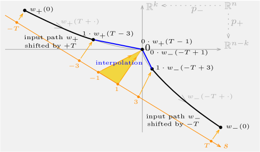
Figure 2: Pre-glued path $w_{T}(s):={\mathcal{P}}_{T}(w_{+},w_{-})(s)$ for $s\in[-T,T]$

Example 2.2 (Constant maps to the critical point).

It holds that

$${\mathcal{P}}_{T}(0_{+},0_{-})=0_{T}.$$ (2.13)

Note that $0_{+}\in{\mathcal{W}}^{\rm s}$, $0_{-}\in{\mathcal{W}}^{\rm u}$, and $0_{T}\in{\mathcal{M}}_{T}$.

Restricted pre-gluing map

We denote the restriction of the pre-gluing map ${\mathcal{P}}_{T}$ to the stable and unstable manifolds ${\mathcal{W}}^{\rm s}\subset{\mathbb{W}}_{+}$ and ${\mathcal{W}}^{\rm u}\subset{\mathbb{W}}_{-}$ by

$$\wp_{T}:={\mathcal{P}}_{T}|_{{\mathcal{W}}^{\rm s}\times{\mathcal{W}}^{\rm u}}\colon{\mathcal{W}}^{\rm s}\times{\mathcal{W}}^{\rm u}\to{\mathbb{W}}_{T}$$ (2.14)

where $T\geq 3$. This map is smooth by linearity of ${\mathcal{P}}_{T}$.

Differential of $\wp_{T}$ at $(0_{+},0_{-})$. Consider the tangent spaces to the trajectory spaces ${\mathcal{W}}^{\rm s}$, ${\mathcal{W}}^{\rm u}$, and ${\mathcal{M}}_{T}$, at the critical point, namely

$$\begin{split}{\mathbb{E}}^{+}:=T_{0_{+}}{\mathcal{W}}^{\rm s}&=\{\xi\in{\mathbb{W}}_{+}\mid{\partial}_{s}\xi+A\xi=0\}\subset C^{\infty}([0,\infty),{\color[rgb]{1,0,0}{\mathbb{R}}^{n-k}\times\{0\}})\\ {\mathbb{E}}^{-}:=T_{0_{-}}{\mathcal{W}}^{\rm u}&=\{\eta\in{\mathbb{W}}_{-}\mid{\partial}_{s}\eta+A\eta=0\}\subset C^{\infty}((-\infty,0],{\color[rgb]{1,0,0}\{0\}\times{\mathbb{R}}^{k}})\\ {\mathbb{E}}_{T}:=T_{0_{T}}{\mathcal{M}}_{T}&=\{\zeta\in{\mathbb{W}}_{T}\mid{\partial}_{s}\zeta+A\zeta=0\}\subset C^{\infty}([-T,T],{\mathbb{R}}^{n}).\end{split}$$ (2.15)

By the theorem of Picard-Lindelöf the dimensions are given by

$$\dim{\mathbb{E}}^{+}=n-k,\qquad\dim{\mathbb{E}}^{-}=k,\qquad\dim{\mathbb{E}}_{T}=n.$$

Then the linearization of $\wp_{T}$ at $(0_{+},0_{-})$ is a map

$$d\wp_{T}(0_{+},0_{-})\colon{\mathbb{E}}^{+}\times{\mathbb{E}}^{-}\to{\mathbb{W}}_{T}.$$

For $\zeta\in{\mathbb{E}}^{+},{\mathbb{E}}^{-},{\mathbb{E}}_{T}$ we abbreviate

$$\zeta^{+}(s):=p_{+}(\zeta(s)),\quad\zeta^{-}(s):=p_{-}(\zeta(s)),\qquad\text{so $\zeta=(\zeta^{+},\zeta^{-})$.}$$ (2.16)

Since $A$ is diagonal, see (1.6), and by decay of the elements of ${\mathbb{W}}_{\pm}$, given maps $\xi\in C^{\infty}([0,\infty),{\mathbb{R}}^{n})$ and $\eta\in C^{\infty}((-\infty,0],{\mathbb{R}}^{n})$, there are the equivalences

$$\begin{split}\xi\in{\mathbb{E}}^{+}\qquad&\Leftrightarrow\qquad\xi=(\xi^{+},0)\quad\wedge\quad\xi^{+}(s)=e^{-sA_{+}}\xi^{+}(0)\;\forall s\geq 0,\\ \eta\in{\mathbb{E}}^{-}\qquad&\Leftrightarrow\qquad\eta=(0,\eta^{-})\quad\wedge\quad\eta^{-}(s)=e^{+sA_{-}}\eta^{-}(0)\;\forall s\leq 0.\end{split}$$ (2.17)

Differential of $\wp_{T}$ at $(w_{+},w_{-})\in{\mathcal{W}}^{\rm s}\times{\mathcal{W}}^{\rm u}$. The tangent spaces to the trajectory spaces ${\mathcal{W}}^{\rm s}$, ${\mathcal{W}}^{\rm u}$, and ${\mathcal{M}}_{T}$, at points $w_{+}$, $w_{-}$, and $w_{T}$, color=yellow!40]${\partial}_{s}$ not $\nabla$! Ableitung im ${\mathbb{R}}^{n}$ are

$$\begin{split}T_{w_{+}}{\mathcal{W}}^{\rm s}&=\{\xi\in{\mathbb{W}}_{+}\mid{\partial}_{s}\xi+A_{w_{+}}\xi=0\}\subset C^{\infty}([0,\infty),{\mathbb{R}}^{n})\\ T_{w_{-}}{\mathcal{W}}^{\rm u}&=\{\eta\in{\mathbb{W}}_{-}\mid{\partial}_{s}\eta+A_{w_{-}}\eta=0\}\subset C^{\infty}((-\infty,0],{\mathbb{R}}^{n})\\ T_{w_{T}}{\mathcal{M}}_{T}&=\{\zeta\in{\mathbb{W}}_{T}\mid{\partial}_{s}\zeta+A_{w_{T}}\zeta=0\}\subset C^{\infty}([-T,T],{\mathbb{R}}^{n}).\end{split}$$ (2.18)

Here, for $w\in\{w_{+},w_{-},w_{T}\}$, the family of Hessian operators

$$A_{w}=\{A_{w}(s)\}_{s}$$

is defined by the identities $\left(\mathrm{Hess}_{w(s)}f\right)(\cdot,\cdot)=g_{w(s)}\left(\cdot,A_{w}(s)\cdot\right)$, one identity for each $s$. There are canonical, continuous and linear, identifications

$$\theta_{w_{+}}\colon{\mathbb{W}}_{+}\supset T_{w_{+}}{\mathcal{W}}^{\rm s}\stackrel{{\scriptstyle\simeq}}{{\longrightarrow}}{\mathbb{E}}^{+},\qquad\theta_{w_{-}}\colon{\mathbb{W}}-\supset T_{w_{-}}{\mathcal{W}}^{\rm u}\stackrel{{\scriptstyle\simeq}}{{\longrightarrow}}{\mathbb{E}}^{-},$$ (2.19)

given by asymptotic limits where $\theta_{0_{\pm}}={\rm Id}_{{\mathbb{E}}^{\pm}}=:{\rm Id}_{\pm}$ and the linear operators $\theta_{w_{\pm}}$ depend continuously on $w_{\pm}$; color=yellow!40]detail this; cf. method ’glattbuegeln’ [Weber:2015c] see [RS01, §3]. Since $\wp_{T}:={\mathcal{P}}_{T}|_{{\mathcal{W}}^{\rm s}\times{\mathcal{W}}^{\rm u}}$ is defined by restricting a linear map, the linearization is the linear map’s restriction

$$d\wp_{T}(w_{+},w_{-})=d\left({\mathcal{P}}_{T}|\right)(w_{+},w_{-})={\mathcal{P}}_{T}|\colon T_{w_{+}}{\mathcal{W}}^{\rm s}\times T_{w_{-}}{\mathcal{W}}^{\rm u}\to{\mathbb{W}}_{T}.$$ (2.20)

Thus, given $(w_{+},w_{-})\in{\mathcal{W}}^{\rm s}\times{\mathcal{W}}^{\rm u}$, the map defined by

$$\begin{split}\Theta_{T}(w_{+},w_{-})\colon{\mathbb{E}}^{+}\times{\mathbb{E}}^{-}&\to{\mathbb{W}}_{T}\\ (\xi,\eta)&\mapsto{\mathcal{P}}_{T}\left(\xi-\theta_{w_{+}}^{-1}\xi,\eta-\theta_{w_{-}}^{-1}\eta\right)\end{split}$$ (2.21)

is, by (2.20), equal to the difference

$$\begin{split}\Theta_{T}(w_{+},w_{-})&={\mathcal{P}}_{T}\left(({\rm Id}_{+},{\rm Id}_{-})-(\theta_{w_{+}}^{-1},\theta_{w_{-}}^{-1})\right)\\ &=d\wp_{T}|_{(0_{+},0_{-})}-d\wp_{T}|_{(w_{+},w_{-})}\circ(\theta_{w_{+}}^{-1},\theta_{w_{-}}^{-1}).\end{split}$$

Lemma 2.3.

For any ${\varepsilon}>0$ there are neighborhoods ${\mathcal{O}}^{+}_{\varepsilon}$ of $0_{+}$ in ${\mathcal{W}}^{\rm s}$ and ${\mathcal{O}}^{-}_{\varepsilon}$ of $0_{-}$ in ${\mathcal{W}}^{\rm u}$ such that for every $T\geq 3$ and every $(w_{+},w_{-})\in{\mathcal{O}}^{+}_{\varepsilon}\times{\mathcal{O}}^{-}_{\varepsilon}$ the operator norm of $\Theta_{T}(w_{+},w_{-})\colon{\mathbb{E}}^{+}\times{\mathbb{E}}^{-}\to{\mathbb{W}}_{T}$ is less or equal ${\varepsilon}$.

Proof.

Lemma 2.1 and continuous dependence of $\theta_{w_{\pm}}$ on $w_{\pm}$ and $\theta_{0_{\pm}}={\rm Id}_{\pm}$. ∎

3 Infinitesimal gluing

3.1 Projection associated to a particular complement

Complement ${\mathbb{K}}_{T}$ of $n$-dimensional linear solution space ${\mathbb{E}}_{T}$

For $T>0$ we choose a Hilbert space complement ${\mathbb{K}}_{T}$ of ${\mathbb{E}}_{T}$ in ${\mathbb{W}}_{T}$ of the form

$${\mathbb{K}}_{T}:=\{\zeta=(\zeta^{+},\zeta^{-})\in{\mathbb{W}}_{T}\mid\text{$\zeta^{+}(-T)=0$,\, $\zeta^{-}(T)=0$}\}.$$ (3.22)

Note that the elements $\zeta$ of ${\mathbb{K}}_{T}$ start at points $\zeta(-T)$ in the negative definite space $\{0\}\times{\mathbb{R}}^{k}$ and end at points $\zeta(T)$ in the positive definite space ${\mathbb{R}}^{n-k}\times\{0\}$. Roughly speaking, the linear subspace ${\mathbb{K}}_{T}$ of ${\mathbb{W}}_{T}$ represents impossible paths for a downward gradient flow. The following lemma tells that ${\rm codim\,}{\mathbb{K}}_{T}=n$.

The complement ${\mathbb{K}}_{T}$ of ${\mathbb{E}}_{T}$ is not necessarily orthogonal. But it has the useful property that the infinitesimal gluing map $\Gamma_{T}$ in (3.26) will not depend on the cutoff function $\beta$ that was used to define the pre-gluing map ${\mathcal{P}}_{T}$ color=yellow!40]${\mathbb{E}}_{T}=\ker D$, ${\mathbb{K}}_{T}={\rm im\,}Q$, ${{\mathchoice{\rm 1\mskip-4.0mul}{\rm 1\mskip-4.0mul}{\rm 1\mskip-4.5mul}{\rm 1\mskip-5.0mul}}}-QD=P_{\ker D,{\rm im\,}Q}=P_{{\mathbb{E}}_{T},{\mathbb{K}}_{T}}$ in (2.11).

Lemma 3.1 (Complement).

a) ${\mathbb{K}}_{T}\mathop{\cap}{\mathbb{E}}_{T}=\{0\}$ and b) ${\mathbb{W}}_{T}={\mathbb{K}}_{T}+{\mathbb{E}}_{T}$.

Proof.

a) Pick $\zeta=(\zeta^{+},\zeta^{-})\in{\mathbb{E}}_{T}$. Then $A(0,\zeta^{-})=(0,-A_{-}\zeta^{-})$ and $A(\zeta^{+},0)=(A_{+}\zeta^{+},0)$. Hence ${\partial}_{s}\zeta^{-}=A_{-}\zeta^{-}$ and ${\partial}_{s}\zeta^{+}=-A_{+}\zeta^{+}$, and therefore

$$\zeta^{-}(s)=e^{(s-T)A_{-}}\zeta^{-}(T),\qquad\zeta^{+}(s)=e^{(-s-T)A_{+}}\zeta^{+}(-T),$$

for every $s\in[-T,T]$. Let $\zeta=(\zeta^{+},\zeta^{-})\in{\mathbb{K}}_{T}\mathop{\cap}{\mathbb{E}}_{T}$. Then $\zeta^{+}(-T)=0$ and $\zeta^{-}(T)=0$, so $\zeta^{+}\equiv 0$ and $\zeta^{-}\equiv 0$ since each one solves a first order ODE. Hence $\zeta=(\zeta^{+},\zeta^{-})\equiv 0$. b) Let $\zeta\in{\mathbb{W}}_{T}$. Then the map defined by $Z(s):=\left(e^{(-s-T)A_{+}}p_{+}\zeta(-T),e^{(s-T)A_{-}}p_{-}\zeta(T)\right)$ is element of ${\mathbb{E}}_{T}$ and the difference $\zeta-Z$ lies in ${\mathbb{K}}_{T}$ since $p_{+}(\zeta-Z)(-T)=0$ and $p_{-}(\zeta-Z)(T)=0$. ∎

Uniform Sobolev estimate

Lemma 3.2.

Let $T\geq 1$. color=green!40]$T\geq 1$ Then any $v\colon[-T,T]\to{\mathbb{R}}$ of class $W^{1,2}$ color=yellow!40]can we get $1$? satisfies

$$\mathopen{\|}v\mathclose{\|}_{\infty}\leq 2\mathopen{\|}v\mathclose{\|}_{1,2}$$ (3.23)

where the norms are over the domain $[-T,T]$.

Estimate (3.23) continues to hold for vector-valued maps $v\colon[-T,T]\to{\mathbb{R}}^{\ell}$ of class $W^{1,2}$ since

$$\mathopen{\|}(v_{1},\dots,v_{\ell})\mathclose{\|}_{\infty}=\max_{i=1,\dots,\ell}\mathopen{\|}v_{i}\mathclose{\|}_{\infty}\leq 2\max_{i=1,\dots,\ell}\mathopen{\|}v_{i}\mathclose{\|}_{1,2}\leq 2\mathopen{\|}v\mathclose{\|}_{W^{1,2}([-T,T],{\mathbb{R}}^{\ell})}.$$

Proof of Lemma 3.2.

The proof has 4 steps.

Step 1. Let $T>0$. Suppose $\mathopen{\|}v\mathclose{\|}_{1,2}\leq 1$ and at $s_{0}\in[-T,T]$ we have $\kappa:=\mathopen{|}v(s_{0})\mathclose{|}>0$. Then for $s\in[-T,T]\cap[s_{0}-\kappa^{2}/4,s_{0}+\kappa^{2}/4]$ it holds $\mathopen{|}v(s)\mathclose{|}\geq\kappa/2$.

Pointwise at $s$ we have

$$\begin{split}\mathopen{|}v(s)\mathclose{|}&=\left|v(s_{0})+\int_{s_{0}}^{s}v^{\prime}(\sigma)\cdot 1\,d\sigma\right|\\ &\geq\mathopen{|}v(s_{0})\mathclose{|}-\sqrt{\int_{s_{0}}^{s}\left(v^{\prime}(\sigma)\right)^{2}\,d\sigma}\sqrt{\int_{s_{0}}^{s}1\,d\sigma}\\ &\geq\kappa-\biggl{(}\underbrace{\int_{-T}^{T}\left(v^{\prime}(\sigma)\right)^{2}\,d\sigma}_{\leq\mathopen{\|}v\mathclose{\|}_{1,2}^{2}\leq 1}\biggr{)}^{1/2}\cdot\sqrt{\mathopen{|}s-s_{0}\mathclose{|}}\\ &\geq\kappa-\sqrt{\mathopen{|}s-s_{0}\mathclose{|}}\\ &\geq\kappa-\sqrt{\kappa^{2}/4}=\kappa/2.\end{split}$$

This proves Step 1.

Step 2. Under the assumption of Step 1 suppose, in addition, the inclusion $[s_{0},s_{0}+1]\subset[-T,T]\cap[s_{0}-\kappa^{2}/4,s_{0}+\kappa^{2}/4]$, then $\mathopen{|}v(s_{0})\mathclose{|}=2$.

To prove Step 2 use Step 1 to obtain that

$$\begin{split}1\geq\mathopen{\|}v\mathclose{\|}_{1,2}^{2}\geq\mathopen{\|}v\mathclose{\|}_{2}^{2}\stackrel{{\scriptstyle\mathrm{inclusion}}}{{\geq}}\int_{s_{0}}^{s_{0}+1}\underbrace{v(\sigma)^{2}}_{\stackrel{{\scriptstyle\rm St.1}}{{\geq}}\kappa^{2}/4}\,d\sigma\geq\kappa^{2}/4.\end{split}$$

Therefore $2\geq\kappa$. In view of the inclusion this implies $2=\kappa:=\mathopen{|}v(s_{0})\mathclose{|}$.

Step 3. Under the assumption of Step 1 suppose, in addition, the inclusion $[s_{0}-1,s_{0}]\subset[-T,T]\cap[s_{0}-\kappa^{2}/4,s_{0}+\kappa^{2}/4]$, then $\mathopen{|}v(s_{0})\mathclose{|}=2$.

The same argument as in Step 2 proves Step 3.

Step 4. Let $T\geq 1$. If $\mathopen{\|}v\mathclose{\|}_{1,2}\leq 1$, then $\mathopen{|}v(s_{0})\mathclose{|}\leq 2$ for every $s_{0}\in[-T,T]$.

The assumption $T\geq 1$ guarantees $[s_{0}-1,s_{0}]\subset[-T,T]$ or $[s_{0},s_{0}+1]\subset[-T,T]$. We argue by contradiction and assume that $\kappa:=\mathopen{|}v(s_{0})\mathclose{|}>2$. Then $[s_{0}-1,s_{0}]$ or $[s_{0},s_{0}+1]$ is contained in the intersection $[-T,T]\cap[s_{0}-\kappa^{2}/4,s_{0}+\kappa^{2}/4]$. Therefore by Step 2 or Step 3 we have $\kappa=2$. Contradiction.

By homogeneity of the norm Step 4 implies Lemma 3.2. ∎

Projection $\Pi_{T}$ onto ${\mathbb{E}}_{T}$ along ${\mathbb{K}}_{T}$

We denote the linear projection in the path space ${\mathbb{W}}_{T}:=W^{1,2}([-T,T],{\mathbb{R}}^{n})$ onto the $n$ dimensional subspace ${\mathbb{E}}_{T}$ along the (not necessarily orthogonal) complement ${\mathbb{K}}_{T}$ by

$$P_{{\mathbb{E}}_{T},{\mathbb{K}}_{T}}\stackrel{{\scriptstyle\text{(\ref{eq:zeta_E})}}}{{=}}\Pi_{T}\colon{\mathbb{W}}_{T}={\mathbb{E}}_{T}\oplus{\mathbb{K}}_{T}\to{\mathbb{E}}_{T}.$$ (3.24)

Lemma 3.3.

The projection $P_{{\mathbb{E}}_{T},{\mathbb{K}}_{T}}$ is given by the map $\Pi_{T}\colon\zeta\mapsto\zeta_{{\mathbb{E}}}$ where

$$\begin{split}\zeta_{\mathbb{E}}(s):=\left(e^{-(s+T)A_{+}}\zeta^{+}(-T),e^{(s-T)A_{-}}\zeta^{-}(T)\right)\end{split}$$ (3.25)

for $s\in[-T,T]$.There is color=green!40]$T\geq 1$ a constant $d=d(a_{1},a_{n})$, depending on the eigenvalues $a_{1}$ and $a_{n}$ of $A$ in (1.4), but independent of $T\geq 1$, such that $\mathopen{\|}\Pi_{T}\mathclose{\|}\leq d$.

Proof.

Let $\zeta\in{\mathbb{W}}_{T}$. The map $\zeta\mapsto\zeta_{\mathbb{E}}$ is linear. Moreover $(\zeta_{\mathbb{E}})_{\mathbb{E}}(s)=\zeta_{\mathbb{E}}(s)$ since $\zeta_{\mathbb{E}}^{+}(-T)=\zeta^{+}(-T)$ and $\zeta_{\mathbb{E}}^{-}(T)=\zeta^{-}(T)$. This proves identity 1 in the following

$$\Pi_{T}\circ\Pi_{T}\stackrel{{\scriptstyle{\color[rgb]{.5,.5,.5}1}}}{{=}}\Pi_{T},\qquad{\rm im\,}\Pi_{T}\stackrel{{\scriptstyle{\color[rgb]{.5,.5,.5}2}}}{{=}}{\mathbb{E}}_{T},\qquad\ker\Pi_{T}\stackrel{{\scriptstyle{\color[rgb]{.5,.5,.5}3}}}{{=}}{\mathbb{K}}_{T}.$$

Identity 2: One readily checks that ${\partial}_{s}\zeta_{\mathbb{E}}=-A\zeta_{\mathbb{E}}$, therefore $\zeta_{\mathbb{E}}\in{\mathbb{E}}_{T}$. Hence ${\rm im\,}\Pi_{T}\subset{\mathbb{E}}_{T}$. Vice versa, given $\zeta\in{\mathbb{E}}_{T}$, the two components $\zeta^{\pm}:=p_{\pm}\zeta$ satisfy for $s\in[-T,T]$, and using (1.4), the ODE ${\partial}_{s}\zeta^{+}=-A_{+}\zeta^{+}$ with initial value $\zeta^{+}(-T)$ at $s=-T$ and the ODE ${\partial}_{s}\zeta^{-}=A_{-}\zeta^{-}$ with initial value $\zeta^{-}(T)$ at $s=T$. The solutions are given by $s\mapsto e^{-(s+T)A_{+}}\zeta^{+}(-T)$ and by $s\mapsto e^{(s-T)A_{-}}\zeta^{-}(T)$, respectively. Their direct sum is $\zeta_{\mathbb{E}}$, hence ${\mathbb{E}}_{T}\subset{\rm im\,}\Pi_{T}$.
Identity 3: Pointwise in $s$ vanishing of the vector valued map $(\Pi_{T}\zeta)(s)=\left(e^{-(s+T)A_{+}}\zeta^{+}(-T),e^{(s-T)A_{-}}\zeta^{-}(T)\right)=(0,0)$ happens iff both components vanish, that is iff $\zeta\in{\mathbb{K}}_{T}$.

To find a bound for $P$, pick $\zeta\in{\mathbb{W}}_{T}$. Straightforward calculation shows that

$$\begin{split}\mathopen{\|}\zeta_{\mathbb{E}}\mathclose{\|}_{{\mathbb{W}}_{T}}^{2}&\stackrel{{\scriptstyle{\color[rgb]{1,1,1}\text{(3.11)}}}}{{=}}\mathopen{\|}\zeta_{\mathbb{E}}\mathclose{\|}_{{\mathbb{V}}_{T}}^{2}+\mathopen{\|}\tfrac{d}{ds}\zeta_{\mathbb{E}}\mathclose{\|}_{{\mathbb{V}}_{T}}^{2}\\ &\stackrel{{\scriptstyle(\ref{eq:zeta_E})}}{{=}}\int_{-T}^{T}\left|\left(e^{-(s+T)A_{+}}\zeta^{+}(-T),e^{(s-T)A_{-}}\zeta^{-}(T)\right)\right|^{2}\,ds\\ &\qquad+\int_{-T}^{T}\left|\left(-A_{+}e^{-(s+T)A_{+}}\zeta^{+}(-T),A_{-}e^{(s-T)A_{-}}\zeta^{-}(T)\right)\right|^{2}\,ds\\ &\stackrel{{\scriptstyle(\ref{eq:p})}}{{=}}\int_{0}^{2T}\left|e^{-sA_{+}}\xi^{+}(-T)\right|^{2}+\left|A_{+}e^{-sA_{+}}\xi^{+}(-T)\right|^{2}\,ds\\ &\qquad+\int_{-2T}^{0}\left|e^{sA_{-}}\zeta^{-}(T)\right|^{2}+\left|A_{-}e^{sA_{-}}\zeta^{-}(T)\right|^{2}\,ds\\ &\stackrel{{\scriptstyle(\ref{eq:A})}}{{=}}\sum_{i=1}^{n-k}\int_{0}^{2T}(1+a_{i}^{2})e^{-2sa_{i}}\zeta_{i}(-T)^{2}\,ds\\ &\qquad+\sum_{j=n-k+1}^{n}\int_{-2T}^{0}(1+a_{j}^{2})e^{-2sa_{j}}\zeta_{j}(T)^{2}\,ds\\ &\stackrel{{\scriptstyle{\color[rgb]{1,1,1}\text{(3.1)}}}}{{=}}\sum_{i=1}^{n-k}(1+a_{i}^{2})\zeta_{i}(-T)^{2}\tfrac{1-e^{-4Ta_{i}}}{2a_{i}}+\sum_{j=n-k+1}^{n}(1+a_{j}^{2})\zeta_{j}(T)^{2}\tfrac{1-e^{4Ta_{j}}}{-2a_{j}}\\ &\stackrel{{\scriptstyle(\ref{eq:A-diag})}}{{\leq}}\tfrac{1+a_{1}^{2}}{2\sigma}\sum_{i=1}^{n-k}\zeta_{i}(-T)^{2}+\tfrac{1+a_{n}^{2}}{2\sigma}\sum_{j=n-k+1}^{n}\zeta_{j}(T)^{2}\\ &\stackrel{{\scriptstyle{\color[rgb]{1,1,1}\text{(3.1)}}}}{{\leq}}\tfrac{d^{2}}{8}\left(\mathopen{|}p_{+}\zeta(-T)\mathclose{|}^{2}+\mathopen{|}p_{-}\zeta(T)\mathclose{|}^{2}\right)\quad{\color[rgb]{.5,.5,.5},\tfrac{d^{2}}{8}:=\tfrac{\max\{{\color[rgb]{1,0,0}1+a_{1}^{2}},1+a_{n}^{2}\}}{2\sigma}}\\ \end{split}$$

$$\begin{split}&\stackrel{{\scriptstyle{\color[rgb]{1,1,1}\text{(3.1)}}}}{{\leq}}\tfrac{d^{2}}{4}\mathopen{\|}\zeta\mathclose{\|}_{L^{\infty}([-T,T])}^{2}\\ &\stackrel{{\scriptstyle(\ref{eq:sob-emb-T})}}{{\leq}}d^{2}\mathopen{\|}\zeta\mathclose{\|}_{{\mathbb{W}}_{T}}^{2}.\end{split}$$

Here equality two is by definition (3.25) of $\zeta_{\mathbb{E}}$. Equality three is by the $g_{0}$-orthogonal splitting (1.5) which makes the mixed inner products zero. Equality four uses that $A={\rm diag}(A_{+},-A_{-})$, by (1.6), and the $a_{i}>0>a_{j}$ are ordered by (1.4). Equality five is by integration. color=yellow!40]can’t do (3.30) – $\zeta$ not ODE solution The first inequality uses the order (1.4) of the matrix entries $a_{\ell}$ and definition (1.7) of the spectral gap $\sigma$. The third inequality uses that the projections $p_{\pm}$ are orthogonal, hence of norm $\leq 1$. The final inequality four is by the, uniform in $T$, Sobolev estimate (3.23). This concludes the proof of Lemma 3.3. ∎

3.2 Infinitesimal gluing map $\Gamma_{T}$

Definition 3.4.

For $T\geq 3$ we call the linear map defined by the composition

$$\Gamma_{T}:=\Pi_{T}\circ d\wp_{T}(0_{+},0_{-})\colon{\mathbb{E}}^{+}\times{\mathbb{E}}^{-}\to{\mathbb{W}}_{T}\to{\mathbb{E}}_{T}$$ (3.26)

the infinitesimal gluing map. It acts as shown in (3.29) and Figure 3.

To obtain a formula for $\Gamma_{T}$ we proceed in three steps I–III. Fix elements $\xi=(\xi^{+},0)\in{\mathbb{E}}^{+}$ and $\eta=(0,\eta^{-})\in{\mathbb{E}}^{-}$; see (2.17).

I. Time $s=-T$: By definition (2.14 of $\wp_{T}$ and (2.11) of the pre-gluing map ${\mathcal{P}}_{T}$ (using that $1-\beta(-T+2)={\color[rgb]{0,1,1}1}$ and $\beta(-T-2)={\color[rgb]{.75,.5,.25}0}$ for $T\geq 3$) we obtain

$$\begin{split}d\wp_{T}(0_{+},0_{-})(\xi,\eta)(-T)&\stackrel{{\scriptstyle(\ref{eq:wp})}}{{=}}\left(\left.\tfrac{d}{d\tau}\right|_{0}{\mathcal{P}}_{T}({\varepsilon}\xi,{\varepsilon}\eta)\right)(-T)\\ &\stackrel{{\scriptstyle(\ref{eq:Pp_T})}}{{=}}{\color[rgb]{0,1,1}1}\cdot\xi(T-T)+{\color[rgb]{.75,.5,.25}\,0}\cdot\eta(-T-T)=(\xi^{+}(0),0).\end{split}$$

In view of the direct sum ${\mathbb{W}}_{T}={\mathbb{K}}_{T}\oplus{\mathbb{E}}_{T}$ and since $\Gamma_{T}(\xi,\eta):=P_{{\mathbb{E}}_{T},{\mathbb{K}}_{T}}\circ d\wp_{T}(0_{+},0_{-})(\xi,\eta)$ is the projection to ${\mathbb{E}}_{T}$ there is an element $\zeta$ in the projection kernel ${\mathbb{K}}_{T}$ such that $d\wp_{T}(0_{+},0_{-})(\xi,\eta)=\zeta+\Gamma_{T}(\xi,\eta)$. So we get identity $1$ in

$$p_{+}\Bigl{(}\Gamma_{T}(\xi,\eta)(-T)\Bigr{)}\stackrel{{\scriptstyle{\color[rgb]{.5,.5,.5}1}}}{{=}}p_{+}\Bigl{(}d\wp_{T}(0_{+},0_{-})(\xi,\eta)(-T)-\zeta(-T)\Bigr{)}\stackrel{{\scriptstyle{\color[rgb]{.5,.5,.5}2}}}{{=}}\xi^{+}(0).$$ (3.27)

Identity $2$ holds as $p_{+}(\zeta(-T))=0$ by condition one in definition (3.22) of ${\mathbb{K}}_{T}$.

II. Time $s=T$: Similarly as in I. we obtain that

$$d\wp_{T}(0_{+},0_{-})(\xi,\eta)(T)\stackrel{{\scriptstyle(\ref{eq:Pp_T})}}{{=}}\eta(0)=(0,\eta^{-}(0)).$$

Now use condition two in definition (3.22) of ${\mathbb{K}}_{T}$ to conclude that

$$p_{-}\left(\Gamma_{T}(\xi,\eta)(T)\right)=\eta^{-}(0).$$ (3.28)

III. Time $s\in[-T,T]$: Since $\Gamma_{T}(\xi,\eta)$ lies in ${\mathbb{E}}_{T}$ it satisfies the ODE given by ${\partial}_{s}\Gamma_{T}(\xi,\eta)+A\Gamma_{T}(\xi,\eta)=0$ and so, by (3.27) and (3.28), we get the formula

$$\Gamma_{T}(\xi,\eta)(s)=\left(e^{-(s+T)A_{+}}\xi^{+}(0),e^{(s-T)A_{-}}\eta^{-}(0)\right).$$ (3.29)

In particular, due to the choice of the complement ${\mathbb{K}}_{T}$ which just involves the ends $-T$ and $T$, the infinitesimal gluing map does not depend on the choice of the cutoff function $\beta$ used to define the pre-gluing map (2.11).

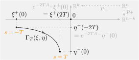
Figure 3: Infinitesimal gluing isomorphism $\Gamma_{T}\in{\mathcal{L}}({\mathbb{E}}^{+}\times{\mathbb{E}}^{-},{\mathbb{E}}_{T})$; cf. (3.29)

Lemma 3.5 (Norm).

Let $T\geq 3$. The linear map $\Gamma_{T}\colon{\mathbb{E}}^{+}\times{\mathbb{E}}^{-}\to{\mathbb{E}}_{T}$ is an isomorphism of norm $\mathopen{\|}\Gamma_{T}\mathclose{\|}\leq 1$ and the norm of the inverse is bounded, uniformly in $T$, color=yellow!40]used in Thm. 5.3 by $k:=1/(1-e^{-12\sigma})$ where $\sigma$ is the spectral gap (1.7) of $A$.

Proof.

We saw that $\dim{\mathbb{E}}^{+}=n-k$, $\dim{\mathbb{E}}^{-}=k$, and $\dim{\mathbb{E}}_{T}=n$. Hence it suffices to show injectivity, i.e. that the kernel of $\Gamma_{T}$ is trivial. Given $(\xi,\eta)\in\ker\Gamma_{T}$, then by (3.29) we have $\xi^{+}(0)=0$ and $\eta^{-}(0)=0$. So $\xi^{+}\equiv 0$ and $\eta^{-}\equiv 0$, since $\xi^{+}$ and $\eta^{-}$ are solutions of a linear first order ODE; see (2.17). Therefore $\xi=(\xi^{+},0)\equiv 0$ and $\eta=(0,\eta^{-})\equiv 0$. This shows that $\Gamma_{T}$ is an isomorphism whenever $T\geq 3$.

To see that $\Gamma_{T}$ and ${\Gamma_{T}}^{-1}$ are bounded, uniformly in $T$, consider the identities

$$\begin{split}\mathopen{\|}\Gamma_{T}(\xi,\eta)\mathclose{\|}_{{\mathbb{W}}_{T}}^{2}&\stackrel{{\scriptstyle{\color[rgb]{1,1,1}\text{(3.11)}}}}{{=}}\mathopen{\|}\Gamma_{T}(\xi,\eta)\mathclose{\|}_{{\mathbb{V}}_{T}}^{2}+\mathopen{\|}\tfrac{d}{ds}\Gamma_{T}(\xi,\eta)\mathclose{\|}_{{\mathbb{V}}_{T}}^{2}\\ &\stackrel{{\scriptstyle(\ref{eq:Gamma_T})}}{{=}}\int_{-T}^{T}\left|\Bigl{(}e^{-(s+T)A_{+}}\xi^{+}(0),e^{(s-T)A_{-}}\eta^{-}(0)\Bigr{)}\right|^{2}\,ds\\ &\qquad+\int_{-T}^{T}\left|\Bigl{(}-A_{+}e^{(-s-T)A_{+}}\xi^{+}(0),A_{-}e^{(s-T)A_{-}}\eta^{-}(0)\Bigr{)}\right|^{2}\,ds\\ &\stackrel{{\scriptstyle(\ref{eq:p})}}{{=}}\int_{0}^{2T}\left|e^{-sA_{+}}\xi^{+}(0)\right|^{2}+\left|A_{+}e^{-sA_{+}}\xi^{+}(0)\right|^{2}\,ds\\ &\qquad+\int_{-2T}^{0}\left|e^{sA_{-}}\eta^{-}(0)\right|^{2}+\left|A_{-}e^{sA_{-}}\eta^{-}(0)\right|^{2}\,ds\\ &\stackrel{{\scriptstyle(\ref{eq:A})}}{{=}}\sum_{i=1}^{n-k}\int_{0}^{2T}(1+a_{i}^{2})e^{-2sa_{i}}\xi_{i}(0)^{2}\,ds\\ &\quad+\sum_{j=n-k+1}^{n}\int_{-2T}^{0}(1+a_{j}^{2})e^{-2sa_{j}}\eta_{j}(0)^{2}\,ds\\ &\stackrel{{\scriptstyle{\color[rgb]{1,1,1}\text{(3.11)}}}}{{=}}\sum_{i=1}^{n-k}(1+a_{i}^{2})\xi_{i}(0)^{2}\tfrac{1-e^{-4Ta_{i}}}{2a_{i}}+\sum_{j=n-k+1}^{n}(1+a_{j}^{2})\eta_{j}(0)^{2}\tfrac{1-e^{4Ta_{j}}}{-2a_{j}}\end{split}$$

where equality two is by formula (3.29) for $\Gamma_{T}$. Equality three is by the $g_{0}$-orthogonal splitting (1.5). Equality four uses that $A={\rm diag}(A_{+},-A_{-})$, by (1.6), and the $a_{i}>0>a_{j}$ are ordered by (1.4). Equality five is by integration.

The ${\mathbb{W}}_{+}$ norm of $\xi=(\xi^{+},0)\in{\mathbb{E}}^{+}$, see (2.17), is given by

$$\begin{split}\mathopen{\|}\xi\mathclose{\|}_{{\mathbb{W}}_{+}}^{2}&\stackrel{{\scriptstyle{\color[rgb]{1,1,1}\text{(3.11)}}}}{{=}}\mathopen{\|}\xi\mathclose{\|}_{{\mathbb{V}}_{+}}^{2}+\mathopen{\|}\tfrac{d}{ds}\xi\mathclose{\|}_{{\mathbb{V}}_{+}}^{2}\\ &\stackrel{{\scriptstyle\text{(\ref{eq:xi-eta-equiv})}}}{{=}}\int_{0}^{\infty}\mathopen{|}e^{-sA_{+}}\xi^{+}(0)\mathclose{|}^{2}\,ds+\int_{0}^{\infty}\mathopen{|}A_{+}e^{-sA_{+}}\xi^{+}(0)\mathclose{|}^{2}\,ds\\ &\stackrel{{\scriptstyle\text{(\ref{eq:A-diag})}}}{{=}}\sum_{i=1}^{n-k}\int_{0}^{\infty}(1+a_{i}^{2})e^{-2sa_{i}}\xi_{i}(0)^{2}\,ds\\ &\stackrel{{\scriptstyle{\color[rgb]{1,1,1}\text{(3.11)}}}}{{=}}\sum_{i=1}^{n-k}\tfrac{1+a_{i}^{2}}{2a_{i}}\xi_{i}(0)^{2}\end{split}$$ (3.30)

and analogously for the ${\mathbb{W}}_{-}$ norm of $\eta=(0,\eta^{-})\in{\mathbb{E}}^{-}$.

To see that ${\Gamma_{T}}^{-1}$ is bounded, uniformly in $T$, we estimate $\Gamma_{T}$ from below

$$\begin{split}\mathopen{\|}\Gamma_{T}(\xi,\eta)\mathclose{\|}_{{\mathbb{W}}_{T}}^{2}&=\sum_{i=1}^{n-k}(1+a_{i}^{2})\xi_{i}(0)^{2}\tfrac{1-e^{-4Ta_{i}}}{2a_{i}}+\sum_{j=n-k+1}^{n}(1+a_{j}^{2})\eta_{j}(0)^{2}\tfrac{1-e^{4Ta_{j}}}{-2a_{j}}\\ &\geq\left(1-e^{-12\sigma}\right)\left(\sum_{i=1}^{n-k}\tfrac{1+a_{i}^{2}}{2a_{i}}\xi_{i}(0)^{2}+\sum_{i=n-k+1}^{n}\tfrac{1+a_{j}^{2}}{-2a_{j}}\eta_{j}(0)^{2}\right)\\ &=\left(1-e^{-12\sigma}\right)\left(\mathopen{\|}\xi\mathclose{\|}_{{\mathbb{W}}_{+}}^{2}+\mathopen{\|}\eta\mathclose{\|}_{{\mathbb{W}}_{-}}^{2}\right).\end{split}$$

To obtain the inequality we use the assumption $T\geq 3$ and the spectral gap $\sigma$ of $A$ defined by (1.7) of $A$. The last equality is explained right above.

To see that $\Gamma_{T}$ is bounded, uniformly in $T$, we estimate $\Gamma_{T}$ from above

$$\begin{split}\mathopen{\|}\Gamma_{T}(\xi,\eta)\mathclose{\|}_{{\mathbb{W}}_{T}}^{2}&=\sum_{i=1}^{n-k}(1+a_{i}^{2})\xi_{i}(0)^{2}\tfrac{1-e^{-4Ta_{i}}}{2a_{i}}+\sum_{j=n-k+1}^{n}(1+a_{j}^{2})\eta_{j}(0)^{2}\tfrac{1-e^{4Ta_{j}}}{-2a_{j}}\\ &\leq\sum_{i=1}^{n-k}\tfrac{1+a_{i}^{2}}{2a_{i}}\xi_{i}(0)^{2}+\sum_{j=n-k+1}^{n}\tfrac{1+a_{j}^{2}}{-2a_{j}}\eta_{j}(0)^{2}\\ &=\mathopen{\|}\xi\mathclose{\|}_{{\mathbb{W}}_{+}}^{2}+\mathopen{\|}\eta\mathclose{\|}_{{\mathbb{W}}_{-}}^{2}\end{split}$$

where the inequality holds since $1-e^{-4Ta_{i}}\leq 1$ and $1-e^{4Ta_{j}}\leq 1$. ∎

4 Newton-Picard map

Given two elements $w_{+}\in{\mathcal{W}}^{\rm s}$ and $w_{-}\in{\mathcal{W}}^{\rm u}$ near the critical point, we view the pre-glued path

$$w_{T}:=\wp_{T}(w_{+},w_{-})\in{\mathbb{W}}_{T}$$

as an approximate flow trajectory, equivalently an approximate zero $x_{1}$ of the section ${\mathcal{F}}_{T}$, and then detect a nearby solution using the implicit function theorem with initial point $x_{0}:=0_{T}$, see Appendix B. Thus we need that ${\mathcal{F}}_{T}(w_{T})$ is suitably close to zero. We also need a uniformly in $T$ bounded right inverse $Q_{T}$ of the linearization $D_{T}:=d{\mathcal{F}}_{T}(0_{T})$. These are the next two subsections.

4.1 Approximate zero

Proposition 4.1 (Pre-glued path is approximate zero).

Pick ${\varepsilon}\in(0,\sigma)$ where $\sigma=\sigma(A)$ is the spectral gap (1.7). Let $m\in{\mathbb{N}}_{0}$ and choose compact neighborhoods $K_{+}=K_{+}(m)$ of $0_{+}\in{\mathcal{W}}^{\rm s}$ in $T^{m}{\mathcal{W}}^{\rm s}$ and $K_{-}=K_{-}(m)$ of $0_{-}\in{\mathcal{W}}^{\rm u}$ in $T^{m}{\mathcal{W}}^{\rm u}$. Then the following is true. Given two elements

$$W_{+}\in K_{+}\subset T^{m}{\mathcal{W}}^{\rm s},\qquad W_{-}\in K_{-}\subset T^{m}{\mathcal{W}}^{\rm u},$$

pre-glue them with the $m$-fold tangent map of $\wp_{T}$, see (2.14), to get

$$W_{T}:=T^{m}\wp_{T}(W_{+},W_{-}).$$

Then there is a constant $C(K_{+},K_{-})$, independent of $T$, such that

$$\begin{split}\left\|T^{m}{\mathcal{F}}_{T}(W_{T})\right\|_{T^{m}{\mathbb{V}}_{T}}\leq C(K_{+},K_{-})\cdot e^{-{\varepsilon}T}\end{split}$$ (4.31)

whenever $T\geq 3$.

Proof.

Let $m\in{\mathbb{N}}_{0}$. An color=yellow!40]$m=0$, $1$ App. LABEL:app:TM element $W_{+}\in T^{m}{\mathcal{W}}^{\rm s}$ is a map satisfying the equation

$$W_{+}\colon[0,\infty)\to T^{m}{\mathbb{R}}^{n},\qquad{\partial}_{s}W_{+}+T^{m}\nabla\kern-2.15277ptf(W_{+})=0.$$ (4.32)

An element $W_{-}\in T^{m}{\mathcal{W}}^{\rm s}$ is a map that satisfies the equation

$$W_{-}\colon(-\infty,0]\to T^{m}{\mathbb{R}}^{n},\qquad{\partial}_{s}W_{-}+T^{m}\nabla\kern-2.15277ptf(W_{-})=0.$$ (4.33)

Since $\mathrm{𝟎}$ is a non-degenerate critical point of $f$ the solutions $W_{+}$ and $W_{-}$ decay with all their derivatives exponentially. color=yellow!40]use:
*uniform* exp. decay In particular, by Theorem C.1 and compactness of $K_{\pm}$, there is a constant $c=c(K_{+},K_{-})$ with

$$\mathopen{|}W_{+}(s)\mathclose{|}+\mathopen{|}{\partial}_{s}W_{+}(s)\mathclose{|}\leq ce^{-{\varepsilon}s},\quad\mathopen{|}W_{-}(s)\mathclose{|}+\mathopen{|}{\partial}_{s}W_{-}(s)\mathclose{|}\leq ce^{{\varepsilon}s},$$ (4.34)

for every $s\geq 0$, respectively $s\leq 0$. Since $f$ has a critical point at the origin, we get $T^{m}\nabla\kern-2.15277ptf(0)=0$ where $0\in T^{m}{\mathbb{R}}^{n}$. Hence there is color=yellow!40]by Taylor a constant $\mu_{m}>0$ with

$$\left|T^{m}\nabla\kern-2.15277ptf(W)\right|\leq\mu_{m}\mathopen{|}W\mathclose{|}$$ (4.35)

whenever $\mathopen{|}W\mathclose{|}\leq c$.

By linearity of the pre-gluing map ${\mathcal{P}}_{T}$, the $m-$fold tangent map is given by

$$\begin{split}W_{T}:=T^{m}{\mathcal{P}}_{T}(W_{+},W_{-})&\stackrel{{\scriptstyle\text{(\ref{eq:Pp_T})}}}{{=}}\left(1-\beta(s+2)\right)W_{+}(T+s)+\beta(s-2)\,W_{-}(-T+s)\end{split}$$

pointwise at $s\in[-T,T]$. Similarly, color=yellow!40]linearity in analogy to (2.12), we have

$$W_{T}(s)=\begin{cases}W_{+}(T+s)&\text{, $s\in[-T,-3]$}\\ \left(1-\beta(s+2)\right)W_{+}(T+s)&\text{, $s\in[-3,-1]$}\\ 0&\text{, $s\in[-1,1]$}\\ \beta(s-2)W_{-}(-T+s)&\text{, $s\in[1,3]$}\\ W_{-}(-T+s)&\text{, $s\in[3,T]$}\end{cases}$$ (4.36)

for $s\in[-T,T]$. The tangent map of ${\mathcal{F}}_{T}(w):={\partial}_{s}w+\nabla\kern-2.15277ptf(w)$ at $W_{T}$ is given by

$$T^{m}{\mathcal{F}}_{T}(W_{T})={\partial}_{s}W_{T}+T^{m}\nabla\kern-2.15277ptf(W_{T}).$$ (4.37)

Now there are three cases.
1) For $s\in[-T,-3]\cup[-1,1]\cup[3,T]$ the map $T^{m}{\mathcal{F}}_{T}(W_{T})$ vanishes:

$$\begin{split}T^{m}{\mathcal{F}}_{T}(W_{T})(s)\stackrel{{\scriptstyle\text{(\ref{eq:zeta_TT2})}}}{{=}}{\partial}_{s}W_{+}(T+s)+T^{m}\nabla\kern-2.15277ptf|_{W_{T}(T+s)}&\stackrel{{\scriptstyle\text{(\ref{eq:TW^s-2})}}}{{=}}0,\quad\forall s\in[-T,-3].\\ T^{m}{\mathcal{F}}_{T}(W_{T})(s)\stackrel{{\scriptstyle\text{(\ref{eq:zeta_TT2})}}}{{=}}{\partial}_{s}W_{-}(-T+s)+T^{m}\nabla\kern-2.15277ptf|_{W_{-}(-T+s)}&\stackrel{{\scriptstyle\text{(\ref{eq:TW^u-2})}}}{{=}}0,\quad\forall s\in[3,T].\\ T^{m}{\mathcal{F}}_{T}(W_{T})(s)=0\quad\text{since}\quad W_{T}(s)&\stackrel{{\scriptstyle\text{(\ref{eq:zeta_TT2})}}}{{=}}0,\quad\forall s\in[-1,1].\end{split}$$

2) For $s\in[-3,-1]$, using (4.37) for $T^{m}{\mathcal{F}}_{T}(W_{T})$ and (4.36) for $W_{T}$, we obtain

$$\begin{split}T^{m}{\mathcal{F}}_{T}(W_{T})(s)&=-\beta^{\prime}(s+2)W_{+}(T+s)+(1-\beta(s+2)){\partial}_{s}W_{+}(T+s)\\ &\qquad+T^{m}\nabla\kern-2.15277ptf|_{(1-\beta(s+2))W_{+}(T+s)}.\end{split}$$

Now, by (4.35) and (4.32), we estimate the pointwise length by

$$\begin{split}&\left|T^{m}{\mathcal{F}}_{T}(W_{T})(s)\right|\\ &\leq\mathopen{\|}\beta^{\prime}\mathclose{\|}_{\infty}\mathopen{|}W_{+}(T+s)\mathclose{|}+\mathopen{|}{\partial}_{s}W_{+}(T+s)\mathclose{|}+\left|T^{m}\nabla f|_{(1-\beta(s+2))W_{+}(T+s)}\right|\\ &\leq\left(\mathopen{\|}\beta^{\prime}\mathclose{\|}_{\infty}+1+\mu_{m}\right)c\cdot e^{-{\varepsilon}(s+T)}.\end{split}$$

3) For $s\in[1,3]$ we obtain analogously the formula

$$\begin{split}T^{m}{\mathcal{F}}_{T}(W_{T})(s)&=-\beta^{\prime}(s-2)W_{-}(-T+s)+\beta(s-2){\partial}_{s}W_{-}(-T+s)\\ &\qquad+T^{m}\nabla\kern-2.15277ptf|_{\beta(s-2)W_{-}(-T+s)}\end{split}$$

and the estimate $\left|T^{m}{\mathcal{F}}_{T}(W_{T})(s)\right|\leq\left(\mathopen{\|}\beta^{\prime}\mathclose{\|}_{\infty}+1+\mu_{m}\right)ce^{{\varepsilon}(-T+s)}$.

Thus for the $L^{2}$ norm we get, by integration, the estimate

$$\begin{split}\left\|T^{m}{\mathcal{F}}_{T}(W_{T})\right\|_{T^{m}{\mathbb{V}}_{T}}^{2}\leq\underbrace{2\left(\mathopen{\|}\beta^{\prime}\mathclose{\|}_{\infty}+1+\mu_{m}\right)^{2}c^{2}\frac{e^{6{\varepsilon}}-e^{2{\varepsilon}}}{{\varepsilon}}}_{=:C(K_{+},K_{-})^{2}}e^{-2{\varepsilon}T}\end{split}$$

where $c=c(K_{+},K_{-})$ and $K_{\pm}$ depend on $m$. This proves Proposition 4.1. ∎

4.2 Surjectivity and right inverse

Surjective linearization at $0_{T}$. Let $T>0$. The linearization at general $w\in{\mathbb{W}}_{T}$ is given by

$$d{\mathcal{F}}_{T}(w)\colon{\mathbb{W}}_{T}\to{\mathbb{V}}_{T},\quad\zeta\mapsto{\partial}_{s}\zeta+A_{w}\zeta,\qquad A_{w}(s):=\nabla\nabla\kern-2.15277ptf(w(s)),$$ (4.38)

where $\nabla\nabla\kern-2.15277ptf(w(s))$ is the Jacobian of the vector field $\nabla\kern-2.15277ptf\colon{\mathbb{R}}^{n}\to{\mathbb{R}}^{n}$ at $w(s)$. The linearization at the origin $0_{T}$, namely the operator

$$D_{T}:=d{\mathcal{F}}_{T}(0_{T})\colon{\mathbb{W}}_{T}={\mathbb{E}}_{T}\oplus{\mathbb{K}}_{T}\to{\mathbb{V}}_{T},\quad\zeta\mapsto{\partial}_{s}\zeta+A\zeta,$$ (4.39)

where $A_{0_{T}}=A={\rm diag}(A_{+},-A_{-})$ is the diagonal block matrix (1.6), is surjective: Given $\eta\in{\mathbb{V}}_{T}$, then the element defined by

$$\zeta(s):=e^{-sA}\left(\zeta_{0}+\int_{0}^{s}e^{\sigma A}\eta(\sigma)\,d\sigma\right),\quad\zeta_{0}\in{\mathbb{R}}^{n},$$ (4.40)

for $s\in[-T,T]$, lies in ${\mathbb{W}}_{T}$ and satisfies $d{\mathcal{F}}_{T}(0_{T})\zeta=\eta$. For ${\mathcal{M}}_{T}:={\mathcal{F}}_{T}^{-1}(0)$ there is the natural inclusion ${\mathbb{E}}_{T}:=T_{0_{T}}{\mathcal{M}}_{T}\subset\ker d{\mathcal{F}}_{T}(0_{T})$. On the other hand, both spaces are determined by the initial conditions which are given by ${\mathbb{R}}^{n}$, thus $\dim{\mathbb{E}}_{T}=n=\dim\ker D_{T}$. Therefore the two spaces coincide

$$\ker D_{T}={\mathbb{E}}_{T}.$$ (4.41)

Since ${\mathbb{K}}_{T}$ is a complement of ${\mathbb{E}}_{T}$, the restriction

$${\color[rgb]{.5,.5,.5}\begin{pmatrix}F_{T}^{+}&0\\ 0&F_{T}^{-}\end{pmatrix}=}\,F_{T}:=d{\mathcal{F}}_{T}(0_{T})|_{{\mathbb{K}}_{T}}{\color[rgb]{.5,.5,.5}\,=\begin{pmatrix}\frac{d}{ds}+A_{+}&0\\ 0&\frac{d}{ds}-A_{-}\end{pmatrix}\biggr{|}_{{\mathbb{K}}_{T}}}\colon{\mathbb{K}}_{T}\to{\mathbb{V}}_{T}$$ (4.42)

is injective, hence a continuous linear bijection. Hence, by the open mapping theorem, the inverse

$${\color[rgb]{.5,.5,.5}\begin{pmatrix}Q_{T}^{+}&0\\ 0&Q_{T}^{-}\end{pmatrix}=}\,Q_{T}:={F_{T}}^{-1}{\color[rgb]{.5,.5,.5}\,=\begin{pmatrix}(F_{T}^{+})^{-1}&0\\ 0&(F_{T}^{-})^{-1}\end{pmatrix}}\colon{\mathbb{V}}_{T}\to{\mathbb{K}}_{T}$$ (4.43)

is also continuous. Thus the map $F_{T}\colon{\mathbb{K}}_{T}\to{\mathbb{V}}_{T}$ is a Hilbert space isomorphism.

Right inverse $Q_{T}$ of $D_{T}$.

Remark 4.2 ($Q_{T}$ is a right inverse of $D_{T}$).

Given $\eta\in{\mathbb{V}}_{T}$, then $\zeta:=Q_{T}\eta\in{\mathbb{K}}_{T}$, hence $d{\mathcal{F}}_{T}(0_{T})\zeta=F_{T}\zeta$. Therefore

$$d{\mathcal{F}}_{T}(0_{T})\circ Q_{T}\eta=F_{T}\circ Q_{T}\eta=\eta.$$

Lemma 4.3.

There is a constant $c$, independent of $T>0$, such that $\mathopen{\|}Q_{T}\mathclose{\|}\leq c$.

Proof.

In the proof we distinguish three cases.

I. $A$ positive definite: In this case $k=0$ and $p_{-}=0$, see (1.5), in particular $a_{1}\geq\dots\geq a_{n}>0$. Thus ${\mathbb{K}}_{T}=\{\xi\in{\mathbb{W}}_{T}\mid\xi(-T)=0\}$; see (3.22). Given $\eta\in{\mathbb{V}}_{T}$, let $\zeta:=Q_{T}\eta$, equivalently $\eta=F_{T}\zeta$. Since $\zeta\in{\mathbb{K}}_{T}$, we know that $\zeta(-T)=0$. By (4.40), where we changed the start of the integration from $\mathrm{𝟎}$ to $-T$, we get the formula

$$\begin{split}\zeta(s)&=e^{-sA}\left(\zeta(-T)+\int_{-T}^{s}e^{\sigma A}\eta(\sigma)\,d\sigma\right)\stackrel{{\scriptstyle\zeta(-T)=0}}{{=}}\int_{-T}^{s}e^{-(s-\sigma)A}\eta(\sigma)\,d\sigma\\ &=\int_{[-T,s]\cup{\color[rgb]{1,0,0}(s,T}]}\phi(s-\sigma)\eta(\sigma)\,d\sigma=(\phi*\eta)(s)\end{split}$$

whenever $s\in[-T,T]$ and where the function $\phi$ is defined by $\phi(r):=e^{-rA}$ for $r\geq 0$, and by $\mathrm{𝟎}$ for $r<0$. Hence, by Young’s inequality, we have

$$\mathopen{\|}\zeta\mathclose{\|}_{2}\leq\mathopen{\|}\phi\mathclose{\|}_{1}\mathopen{\|}\eta\mathclose{\|}_{2}\leq\frac{1}{a_{n}}\mathopen{\|}\eta\mathclose{\|}_{2}$$

where the $L^{2}$ and $L^{1}$ norms are over $[-T,T]$ and since

$$\begin{split}\mathopen{\|}\phi\mathclose{\|}_{1}=\int_{-T}^{T}\mathopen{\|}\phi(s)\mathclose{\|}_{{\mathcal{L}}({\mathbb{R}}^{n})}\,ds&=\int_{0}^{T}\mathopen{\|}e^{-sA}\mathclose{\|}_{{\mathcal{L}}({\mathbb{R}}^{n})}\,ds\\ &=\int_{0}^{T}e^{-sa_{n}}\,ds=\tfrac{1-e^{-a_{n}T}}{a_{n}}\leq\tfrac{1}{a_{n}}.\end{split}$$

Note that $a_{n}>0$ is the smallest eigenvalue of the positive definite operator $A$. Since ${\partial}_{s}\zeta=\eta-A\zeta$, and by the triangle inequality and $\mathopen{\|}\zeta\mathclose{\|}_{2}\leq\frac{1}{a_{n}}\mathopen{\|}\eta\mathclose{\|}_{2}$, color=yellow!40] $\mathopen{\|}A\zeta\mathclose{\|}_{2}\leq\mathopen{\|}\phi\mathclose{\|}_{1}\mathopen{\|}A\eta\mathclose{\|}_{2}$

$\mathopen{\|}A\eta\mathclose{\|}_{2}^{2}\leq a_{1}^{2}\mathopen{\|}\eta_{1}\mathclose{\|}_{2}^{2}+\dots+a_{n}^{2}\mathopen{\|}\eta_{n}\mathclose{\|}_{2}^{2}$ $\leq a_{1}^{2}\mathopen{\|}\eta\mathclose{\|}_{2}^{2}$ we get

$$\begin{split}\mathopen{\|}Q_{T}\eta\mathclose{\|}_{1,2}^{2}=\mathopen{\|}\zeta\mathclose{\|}_{1,2}^{2}&=\mathopen{\|}{\partial}_{s}\zeta\mathclose{\|}_{2}^{2}+\mathopen{\|}\zeta\mathclose{\|}_{2}^{2}\\ &=\mathopen{\|}\eta-A\zeta\mathclose{\|}_{2}^{2}+\mathopen{\|}\zeta\mathclose{\|}_{2}^{2}\\ &\leq(\mathopen{\|}\eta\mathclose{\|}_{2}+\mathopen{\|}A\zeta\mathclose{\|}_{2})^{2}+\mathopen{\|}\zeta\mathclose{\|}_{2}^{2}\\ &\leq\left(1+\tfrac{a_{1}}{a_{n}}\right)^{2}\mathopen{\|}\eta\mathclose{\|}_{2}^{2}+\tfrac{1}{a_{n}^{2}}\mathopen{\|}\eta\mathclose{\|}_{2}^{2}.\end{split}$$

This proves Step 1 for $c^{2}=\frac{(a_{1}+a_{n})^{2}+1}{a_{n}^{2}}$.

II. $A$ negative definite: So $k=n$ and $p_{-}={{\mathchoice{\rm 1\mskip-4.0mul}{\rm 1\mskip-4.0mul}{\rm 1\mskip-4.5mul}{\rm 1\mskip-5.0mul}}}$ and ${\mathbb{K}}_{T}=\{\xi\in{\mathbb{W}}_{T}\mid\xi(T)=0\}$. Given $\eta\in{\mathbb{V}}_{T}$, let $\zeta:=Q_{T}\eta$, equivalently $\eta=F_{T}\zeta$. Since $\zeta\in{\mathbb{K}}_{T}$, we know that $\zeta(T)=0$. By (4.40), where we changed the start of the integration from $\mathrm{𝟎}$ to $T$, we obtain the formula

$$\begin{split}\zeta(s)&=e^{sA}\left(\zeta(T)+\int_{T}^{s}e^{-\sigma A}\eta(\sigma)\,d\sigma\right)\stackrel{{\scriptstyle\zeta(T)=0}}{{=}}-\int_{s}^{T}e^{(s-\sigma)A}\eta(\sigma)\,d\sigma\\ &=-\int_{{\color[rgb]{1,0,0}[-T,s)}\cup[s,T]}\phi(s-\sigma)\eta(\sigma)\,d\sigma=-(\phi*\eta)(s)\end{split}$$

whenever $s\in[-T,T]$ and where $\phi$ was defined in Step 1. Continue as in Step 1.

III. General case: Given $\eta=(\eta^{+},\eta^{-})\in{\mathbb{V}}_{T}$. Let $\zeta:=Q_{T}\eta$, then

$$\zeta=(\zeta^{+},\zeta^{-}),\qquad\zeta^{+}=Q_{T}^{+}\eta^{+},\quad\zeta^{-}=Q_{T}^{-}\eta^{-}.$$

From Step I and Step II there exists a constant $c>0$ such that $\mathopen{\|}\zeta^{+}\mathclose{\|}_{1,2}\leq c\mathopen{\|}\eta^{+}\mathclose{\|}_{2}$ and $\mathopen{\|}\zeta^{-}\mathclose{\|}_{1,2}\leq c\mathopen{\|}\eta^{-}\mathclose{\|}_{2}$. Since the splitting ${\mathbb{R}}^{n-k}\times{\mathbb{R}}^{k}$ is orthogonal, we have

$$\mathopen{\|}\zeta\mathclose{\|}_{1,2}^{2}\stackrel{{\scriptstyle\perp}}{{=}}\mathopen{\|}\zeta^{+}\mathclose{\|}_{1,2}^{2}+\mathopen{\|}\zeta^{-}\mathclose{\|}_{1,2}^{2}\leq c^{2}\mathopen{\|}\eta^{+}\mathclose{\|}_{2}^{2}+c^{2}\mathopen{\|}\eta^{-}\mathclose{\|}_{2}^{2}\stackrel{{\scriptstyle\perp}}{{=}}c^{2}\mathopen{\|}\eta\mathclose{\|}_{2}^{2}.$$

This proves Step III and Lemma 4.3. ∎

4.3 Definition of ${\mathcal{N}}_{T}$

Let $c$ be the right inverse bound from Lemma 4.3. In order to use later on Remark B.8 to satisfy hypothesis (B.82), as opposed to only (B.70), we define, for $\mu\geq 2$, a nested family color=yellow!40]HERE $\mu$ APPEARS of open neighborhoods of $\mathrm{𝟎}$ in ${\mathbb{R}}^{n}$ as the pre-image of $[0,1/\mu c)$ under the continuous map $\mathopen{\|}d\nabla\kern-2.15277ptf(\cdot)-A\mathclose{\|}\colon{\mathbb{R}}^{n}\to[0,\infty)$, in symbols

$$B^{\mu}:=\left\|d\nabla\kern-2.15277ptf(\cdot)-A\right\|^{-1}[0,\tfrac{1}{\mu c}),\quad B^{\mu}\subset B^{2}.$$

For $T>0$ define an open neighborhood ${\mathcal{B}}^{\mu}_{T}$ of $0_{T}$ in ${\mathbb{W}}_{T}$ color=green!40]${\mathcal{B}}^{\mu}_{T}$ defined by

$${\mathcal{B}}^{\mu}_{T}:=\{w\in{\mathbb{W}}_{T}\mid w(s)\in B^{\mu}\;\forall s\in[-T,T]\}\subset{\mathcal{B}}^{2}_{T}.$$

Lemma 4.4.

Let $T>0$ and $\mu\geq 2$. If $w\in{\mathcal{B}}^{\mu}_{T}$, then $\mathopen{\|}d{\mathcal{F}}_{T}(w)-D_{T}\mathclose{\|}\leq\frac{1}{\mu c}$.

Proof.

Given $w\in{\mathcal{B}}^{\mu}_{T}$, there is the estimate

$$\mathopen{\|}(d{\mathcal{F}}_{T}(w)-D_{T})\zeta\mathclose{\|}_{2}\stackrel{{\scriptstyle(\ref{eq:dFf})}}{{=}}\mathopen{\|}(d\nabla\kern-2.15277ptf(w)-A)\zeta\mathclose{\|}_{2}\leq\tfrac{1}{\mu c}\mathopen{\|}\zeta\mathclose{\|}_{2}\leq\tfrac{1}{\mu c}\mathopen{\|}\zeta\mathclose{\|}_{1,2}$$

for every $\zeta\in{\mathbb{W}}_{T}$. ∎

Corollary 4.5 (to Lemma 3.2).

There is a monotone decreasing function $\delta\colon[2,\infty)\to(0,\infty)$, $\mu\mapsto\delta(\mu)=:\delta_{\mu}$, independent of $T$, such that for $\mu\in[2,\infty)$ the $\delta_{\mu}$-ball about $0_{T}$ in ${\mathbb{W}}_{T}$ is contained in ${\mathcal{B}}^{\mu}_{T}$, in symbols $B_{\delta_{\mu}}(0_{T};{\mathbb{W}}_{T})\subset{\mathcal{B}}^{\mu}_{T}$.

Proof.

By Lemma 3.2 for $w\in B_{\delta_{\mu}}(0_{T};{\mathbb{W}}_{T})$ we have $\mathopen{\|}w\mathclose{\|}_{\infty}\leq 2\delta_{\mu}$. ∎

Definition 4.6 (Newton-Picard map).

Let $c>0$ be the right inverse bound of Lemma 4.3 and let

$$\delta:=\delta_{4}>0$$ (4.44)

be the value in Corollary 4.5 for $\mu=4$. For $T\geq 1$ we can now, in view of Lemma 4.4 with $\mu=4$ and the McDuff-Salamon Proposition B.1 with $x_{0}=0_{T}$, define a Newton-Picard map

$${\mathcal{N}}_{T}\colon{\mathbb{W}}_{T}\supset{\mathcal{B}}^{4}_{T}\supset U_{0}(\delta)\stackrel{{\scriptstyle\text{(\ref{eq:U_0(delta)})}}}{{:=}}\Bigl{(}B_{\frac{\delta}{8}}(0_{T};{\mathbb{W}}_{T})\cap\left\{\mathopen{\|}{\mathcal{F}}_{T}\mathclose{\|}<\tfrac{\delta}{4c}\right\}\Bigr{)}\to{\mathbb{W}}_{T}.$$ (4.45)

Here the inclusion $U_{0}(\delta)\subset{\mathcal{B}}^{4}_{T}$ holds by Corollary 4.5.

By (B.72) the Newton-Picard map ${\mathcal{N}}_{T}$ enjoys the following properties:

$${\mathcal{F}}_{T}\circ{\mathcal{N}}_{T}(w)=0,\qquad{\mathcal{N}}_{T}(w)-w\in{\rm im\,}Q_{T},\qquad{\mathcal{N}}_{T}(w)\in B_{\delta}(0_{T};{\mathbb{W}}_{T}),$$

and, moreover, one has the estimate

$$\mathopen{\|}({\mathcal{N}}_{T}-{\rm id})(w)\mathclose{\|}_{{\mathbb{W}}_{T}}\leq 2c\mathopen{\|}{\mathcal{F}}_{T}(w)\mathclose{\|}_{{\mathbb{V}}_{T}}.$$ (4.46)

Furthermore, by Corollary B.7, respectively identity (5.53)), we have

$${\mathcal{N}}_{T}(0_{T})=0_{T},\qquad d{\mathcal{N}}_{T}|_{0_{T}}\stackrel{{\scriptstyle\text{(\ref{eq:1-P})}}}{{=}}\Pi_{T},$$ (4.47)

where the projection $\Pi_{T}$, see (3.24), is uniformly bounded in $T$, by Lemma 3.3.

Pre-gluing takes values in domain of Newton-Picard map

The next lemma and Proposition 4.1 show that, for $T\geq 3$ large enough, the pre-gluing map ${\mathcal{P}}_{T}$ takes values in the domain of the Newton-Picard map ${\mathcal{N}}_{T}$.

Lemma 4.7 (The neighborhoods ${\mathcal{U}}^{\mu}_{\pm}$.).

Let $\delta\colon[2,\infty)\to(0,\infty)$, $\mu\mapsto\delta_{\mu}$, be the monotone decreasing function in Corollary 4.5. We abbreviate $\delta:=\delta_{4}$. Then there exists a nested family of open and bounded neighborhoods ${\mathcal{U}}^{\mu}_{+}\subset{\mathcal{W}}^{\rm s}$ of $0_{+}$ and ${\mathcal{U}}^{\mu}_{-}\subset{\mathcal{W}}^{\rm u}$ of $0_{-}$ such that $\mathopen{\|}{\mathcal{P}}_{T}(w_{+},w_{-})\mathclose{\|}_{1,2}<\min\{\frac{\delta}{8},\delta_{\mu}\}$ whenever $\mu\geq 2$, $w_{+}\in{\mathcal{U}}^{\mu}_{+}$, $w_{-}\in{\mathcal{U}}^{\mu}_{-}$, and $T\geq 3$.

While the estimate by $\frac{\delta}{8}$ serves in (4.45), the estimate by $\delta_{\mu}$ for some $\mu\geq 5$ will be used in the proof of Theorem 5.3 further below.

Proof.

For $\delta^{\prime}>0$ let $B_{\delta^{\prime}}(0_{+})\subset{\mathbb{W}}_{+}$ be the open radius $\delta^{\prime}$ ball about $0_{+}$, analogously for $B_{\delta^{\prime}}(0_{-})$. Pick $w_{+}\in B_{\delta^{\prime}}(0_{+})\cap{\mathcal{W}}^{\rm s}$ and $w_{-}\in B_{\delta^{\prime}}(0_{-})\cap{\mathcal{W}}^{\rm u}$ and, for $T\geq 3$, abbreviate $w_{T}:={\mathcal{P}}_{T}(w_{+},w_{-})\colon[-T,T]\to{\mathbb{R}}^{n}$. Since by (2.12) at each time $s$ at most one of $w_{+}(T+s)$ and $w_{-}(-T+s)$ comes with a nonzero factor, we obtain inequality one in the following estimate

$$\begin{split}&\mathopen{\|}w_{T}\mathclose{\|}_{1,2}^{2}\\ &=\mathopen{\|}w_{T}\mathclose{\|}_{2}^{2}+\mathopen{\|}{\partial}_{s}w_{T}\mathclose{\|}_{2}^{2}\\ &\leq\mathopen{\|}w_{+}\mathclose{\|}_{2}^{2}+\mathopen{\|}w_{-}\mathclose{\|}_{2}^{2}+2\mathopen{\|}\beta^{\prime}\mathclose{\|}_{\infty}^{2}\left(\mathopen{\|}w_{+}\mathclose{\|}_{2}^{2}+\mathopen{\|}w_{-}\mathclose{\|}_{2}^{2}\right)+2\left(\mathopen{\|}{\partial}_{s}w_{+}\mathclose{\|}_{2}^{2}+\mathopen{\|}{\partial}_{s}w_{-}\mathclose{\|}_{2}^{2}\right)\\ &\leq 2(1+\mathopen{\|}\beta^{\prime}\mathclose{\|}_{\infty}^{2})\left(\mathopen{\|}w_{+}\mathclose{\|}_{1,2}^{2}+\mathopen{\|}w_{-}\mathclose{\|}_{1,2}^{2}\right)\\ &\leq 4(1+\mathopen{\|}\beta^{\prime}\mathclose{\|}_{\infty}^{2})(\delta^{\prime})^{2}.\\ \end{split}$$

Choose $\delta^{\prime}=\delta^{\prime}(\mu):=\frac{1}{4}\min\{\frac{\delta}{8},\delta_{\mu}\}\sqrt{1+\mathopen{\|}\beta^{\prime}\mathclose{\|}_{\infty}^{2}}$ and define the open $\delta^{\prime}$-neighborhoods in the stable, respectively unstable, manifolds as follows

$${\mathcal{U}}^{\mu}_{+}:=\left(B_{\delta^{\prime}}(0_{+})\cap{\mathcal{W}}^{\rm s}\right)\subset{\mathcal{U}}_{+}:={\mathcal{U}}^{2}_{+},\quad{\mathcal{U}}^{\mu}_{-}:=\left(B_{\delta^{\prime}}(0_{-})\cap{\mathcal{W}}^{\rm u}\right)\subset{\mathcal{U}}_{-}:={\mathcal{U}}^{2}_{-}.$$

Then the lemma holds by the previous displayed estimate. ∎

5 Gluing

Pick ${\varepsilon}\in(0,\sigma)$ where $\sigma=\sigma(A)$ is the spectral gap (1.7). Let $c>0$ be the constant in the right inverse estimate, Lemma 4.3. Let $\delta=\delta_{4}>0$ be the constant in Corollary 4.5 and let

$${\mathcal{U}}_{+/-}:={\mathcal{U}}^{2}_{+/-}\subset{\mathcal{W}}^{\rm s/u},\qquad K_{\pm}:={\rm cl\,}{\mathcal{U}}_{\pm},$$ (5.48)

be the open sets in Lemma 4.7 and, respectively, the compact sets given by the closure of ${\mathcal{U}}_{\pm}$ in the (finite dimensional) stable/unstable manifold. Thus, by Proposition 4.1 for $m=0$, we get a constant $C=C(K_{+},K_{-})>0$. Pick $T_{0}\geq 3$ such that

$$Ce^{-{\varepsilon}T_{0}}<\frac{\delta}{4c}$$ (5.49)

see (4.31). By Proposition 4.1 for $m=0$ and Lemma 4.7 it holds that

$$\mathopen{\|}{\mathcal{F}}_{T}\circ\wp_{T}(w_{+},w_{-})\mathclose{\|}\stackrel{{\scriptstyle(\ref{eq:T^mFf-decay})}}{{<}}\tfrac{\delta}{4c},\qquad\mathopen{\|}\wp_{T}(w_{+},w_{-})\mathclose{\|}<\tfrac{\delta}{8},$$ (5.50)

whenever $T\geq T_{0}$ and $w_{\pm}\in{\mathcal{U}}_{\pm}$ and were $\wp_{T}:={\mathcal{P}}_{T}|_{{\mathcal{W}}^{\rm s}\times{\mathcal{W}}^{\rm u}}\colon{\mathcal{W}}^{\rm s}\times{\mathcal{W}}^{\rm u}\to{\mathbb{W}}_{T}$, see (2.14), is the restriction of the (linear) pre-gluing map ${\mathcal{P}}_{T}\colon{\mathbb{W}}_{+}\times{\mathbb{W}}_{-}\to{\mathbb{W}}_{T}$, see (2.11). In other words, the pre-gluing map $\wp_{T}$ maps ${\mathcal{U}}_{+}\times{\mathcal{U}}_{-}$ into the domain of the Newton-Picard map ${\mathcal{N}}_{T}$, see (4.45), whenever $T\geq T_{0}$.

Definition 5.1 (Gluing map).

For $T\geq T_{0}$ the gluing map is the composition of smooth maps

$$\gamma_{T}:={\mathcal{N}}_{T}\circ\wp_{T}\colon{\mathcal{U}}_{+}\times{\mathcal{U}}_{-}\longrightarrow U_{0}(\delta)\longrightarrow{\mathbb{W}}_{T}.$$ (5.51)

The linearized gluing map is the composition

$$d\gamma_{T}|_{(w_{+},w_{-})}=d{\mathcal{N}}_{T}|_{\wp_{T}(w_{+},w_{-})}\circ d\wp_{T}|_{(w_{+},w_{-})}\colon T_{w_{+}}{\mathcal{W}}^{\rm s}\times T_{w_{-}}{\mathcal{W}}^{\rm u}\to{\mathbb{W}}_{T}.$$

Lemma 5.2.

It holds $\gamma_{T}(0_{+},0_{-})=0_{T}$. Furthermore, the differential of the gluing map $\gamma_{T}$ at $(0_{+},0_{-})$ is the infinitesimal gluing map $\Gamma_{T}$, in symbols

$$d\gamma_{T}|_{(0_{+},0_{-})}=\Pi_{T}\circ d\wp_{T}|_{(0_{+},0_{-})}\stackrel{{\scriptstyle(\ref{eq:Gamma_T-def})}}{{=:}}\Gamma_{T}\colon{\mathbb{E}}^{+}\times{\mathbb{E}}^{-}\to{\mathbb{E}}_{T}.$$

Proof.

We get that $\gamma_{T}(0_{+},0_{-})\stackrel{{\scriptstyle(\ref{eq:0_T})}}{{=}}{\mathcal{N}}_{T}(\wp_{T}(0_{+},0_{-}))\stackrel{{\scriptstyle(\ref{eq:NP-0_T})}}{{=}}{\mathcal{N}}_{T}(0_{T})=0_{T}$.

By definition of $\gamma_{T}$ and the chain rule we get the first equality

$$\begin{split}d\gamma_{T}|_{(0_{+},0_{-})}&=d{\mathcal{N}}_{T}|_{\underbrace{\wp_{T}(0_{+},0_{-})}_{\text{$=0_{T}$ by~{}(\ref{eq:0_T})}}}\circ d\wp_{T}|_{(0_{+},0_{-})}\\ &=\left({\rm Id}-Q_{T}D_{T}\right)\circ d\wp_{T}|_{(0_{+},0_{-})}\\ &=\Pi_{T}\circ d\wp_{T}|_{(0_{+},0_{-})}\\ &=:\Gamma_{T}\end{split}$$ (5.52)

and the second equality holds since $d{\mathcal{N}}_{T}(0_{T})={\rm Id}-Q_{T}D_{T}$, by Corollary B.7 with $x_{0}=0_{T}$ and $P=Q_{T}D_{T}$.
Now $\Pi_{T}\colon{\mathbb{W}}_{T}\to{\mathbb{W}}_{T}$ is the projection onto ${\mathbb{E}}_{T}$ along ${\mathbb{K}}_{T}$, by definition (3.24), in symbols $\Pi_{T}=P_{{\mathbb{E}}_{T},{\mathbb{K}}_{T}}$. Thus, to see that

$${\color[rgb]{.5,.5,.5}d{\mathcal{N}}_{T}(0_{T})=\,}{\rm Id}-Q_{T}D_{T}=P_{{\mathbb{E}}_{T},{\mathbb{K}}_{T}}{\color[rgb]{.5,.5,.5}\,=:\Pi_{T}},$$ (5.53)

it remains to show that the composition

$$Q_{T}D_{T}=P_{{\mathbb{K}}_{T},{\mathbb{E}}_{T}}$$

is the projection onto ${\mathbb{K}}_{T}$ along ${\mathbb{E}}_{T}$. This follows since

$$Q_{T}D_{T}\stackrel{{\scriptstyle\rm(\ref{eq:Q_T})}}{{=}}F_{T}^{-1}d{\mathcal{F}}_{T}|_{0_{T}}=\left(d{\mathcal{F}}_{T}|_{0_{T}}|_{{\mathbb{K}}_{T}}\right)^{-1}d{\mathcal{F}}_{T}|_{0_{T}}\colon W_{T}\to{\mathbb{V}}_{T}\to{\mathbb{K}}_{T}$$

and ${\mathbb{E}}_{T}=\ker d{\mathcal{F}}_{T}|_{0_{T}}=\ker D_{T}$ and $Q_{T}=F_{T}^{-1}\colon{\mathbb{V}}_{T}\to{\mathbb{K}}_{T}$ where $F_{T}$ is the restriction of $D_{T}$ to ${\mathbb{K}}_{T}$, see (4.42). ∎

5.1 Diffeomorphism onto image

Theorem 5.3.

There are open neighborhoods ${\mathcal{O}}_{+}\subset{\mathcal{U}}_{+}\subset{\mathcal{W}}^{\rm s}$ of $0_{+}$ and ${\mathcal{O}}_{-}\subset{\mathcal{U}}_{-}\subset{\mathcal{W}}^{\rm u}$ of $0_{-}$ color=yellow!40]key point: domain indep. of $T$!! such that for every $T\geq T_{0}$ the restricted gluing map

$$\gamma_{T}\colon{\mathcal{O}}_{+}\times{\mathcal{O}}_{-}\to{\mathcal{M}}_{T},\quad(w_{+},w_{-})\mapsto{\mathcal{N}}_{T}\circ\wp_{T}(w_{+},w_{-})$$

is a diffeomorphism onto its image ${\mathcal{O}}_{T}$.

Note that the domain ${\mathcal{O}}_{+}\times{\mathcal{O}}_{-}$ of $\gamma_{T}$ does not depend on $T$.

Proof.

Given $T_{0}\geq 3$ as prior to (5.50), pick $T\geq T_{0}$. The theorem is a consequence of the quantitative inverse function Theorem A.1 (IFT), where $F$ is given by a representative of $\gamma_{T}$ in local coordinate charts; see (2.19). color=yellow!40]more loc. triv. than loc. coords.!! In order to apply the quantitative IFT two conditions, (A.65) and (A.66), are to be checked.

We verify (A.65): Recall that the inverse of the infinitesimal gluing map $\Gamma_{T}$ is uniformly bounded by a constant $k=1/(1-e^{-12\sigma})>1$, see Lemma 3.5. So, by Lemma 5.2, the inverse of $d\gamma_{T}|_{(0_{+},0_{-})}=dF|_{0}$ is bounded by $k$, uniformly in $T$.

We verify (A.66): color=yellow!40]${\varepsilon}=1/8kd$ $\mu=4k+1$ To check this condition we choose

$$\boxed{{\mathcal{O}}_{\pm}:={\mathcal{O}}^{\pm}_{1/8kd}\cap{\mathcal{U}}_{\pm}^{4k+1},}\qquad{\varepsilon}=\tfrac{1}{8kd},\quad\mu=4k+1\geq 5,$$ (5.54)

where $d$ is the ($T$-independent) bound of $\Pi_{T}$ from Lemma 3.3 and where the open origin neighborhoods ${\mathcal{O}}^{\pm}_{\varepsilon}$ and ${\mathcal{U}}_{\pm}^{\mu}$ in ${\mathcal{W}}^{\rm s/u}$ were defined in Lemma 2.3 and Lemma 4.7, respectively. Since $k\geq 1$, Lemma 4.7 tells that ${\mathcal{U}}_{\pm}^{4k+1}\subset{\mathcal{U}}_{\pm}^{2}=:{\mathcal{U}}_{\pm}$, hence ${\mathcal{O}}_{\pm}\subset{\mathcal{U}}_{\pm}$. Pick $(w_{+},w_{-})\in{\mathcal{O}}_{+}\times{\mathcal{O}}_{-}\subset{\mathcal{U}}_{+}\times{\mathcal{U}}_{-}$.

Recalling (2.19) we shall investigate the operator norm of the difference

$$\begin{split}d\gamma_{T}|_{(w_{+},w_{-})}\circ(\theta_{w_{+}}^{-1},\theta_{w_{-}}^{-1})-d\gamma_{T}|_{(0_{+},0_{-})}\colon{\mathbb{E}}^{+}\times{\mathbb{E}}^{-}\to{\mathbb{W}}_{T}.\end{split}$$

Abbreviate $x_{1}:=\wp_{T}(w_{+},w_{-})$. By definition of $\gamma_{T}$ and of $\Theta_{T}(w_{+},w_{-})$ we get

$$\begin{split}&d\gamma_{T}|_{(w_{+},w_{-})}\circ(\theta_{w_{+}}^{-1},\theta_{w_{-}}^{-1})-d\gamma_{T}|_{(0_{+},0_{-})}\\ &\stackrel{{\scriptstyle\text{(\ref{eq:gamma_T})}}}{{=}}d{\mathcal{N}}_{T}|_{x_{1}}\circ{\mathcal{P}}_{T}\circ(\theta_{w_{+}}^{-1},\theta_{w_{-}}^{-1})-d{\mathcal{N}}_{T}|_{0_{T}}\circ{\mathcal{P}}_{T}{\color[rgb]{.5,.5,.5}\;-d{\mathcal{N}}_{T}|_{x_{1}}\circ{\mathcal{P}}_{T}+d{\mathcal{N}}_{T}|_{x_{1}}\circ{\mathcal{P}}_{T}}\\ &\stackrel{{\scriptstyle\text{(\ref{eq:Theta_T})}}}{{=}}-d{\mathcal{N}}_{T}|_{x_{1}}\circ\Theta_{T}(w_{+},w_{-})+\left(d{\mathcal{N}}_{T}|_{x_{1}}-d{\mathcal{N}}_{T}|_{0_{T}}\right)\circ{\mathcal{P}}_{T}.\end{split}$$ (5.55)

By Remark B.5 for $Q:=Q_{T}$ and $P:=Q_{T}D_{T}$ and since the projection ${\rm Id}-P=\Pi_{T}$, see (5.53), has a ($T$-independent) bound $d$ by Lemma 3.3 we get that

$$\mathopen{\|}d{\mathcal{N}}_{T}|_{x_{1}}\mathclose{\|}\stackrel{{\scriptstyle\text{(\ref{eq:dNn})}}}{{\leq}}\mathopen{\|}\left({\rm Id}+Q_{T}\,df(x_{1})-P\right)^{-1}\mathclose{\|}\cdot\mathopen{\|}{\rm Id}-P\mathclose{\|}\stackrel{{\scriptstyle\text{(\ref{eq:inverse-2})}}}{{\leq}}2d.$$ (5.56)

Since $(w_{+},w_{-})\in{\mathcal{O}}^{+}_{1/8kd}\times{\mathcal{O}}^{-}_{1/8kd}$, by Lemma 2.3, we have that

$$\mathopen{\|}\Theta_{T}(w_{+},w_{-})\mathclose{\|}\leq\tfrac{1}{8kd}.$$ (5.57)

Furthermore, abbreviating $x_{0}:=0_{T}$, then $d{\mathcal{N}}_{T}|_{0_{T}}={\rm Id}-P$ by (B.79) with $x_{1}$ replaced by $x_{0}$ and using that $Q_{T}\,df(x_{0})=Q_{T}D_{T}=P$. Thus we get that

$$\left(d{\mathcal{N}}_{T}|_{x_{1}}-d{\mathcal{N}}_{T}|_{0_{T}}\right)\circ{\mathcal{P}}_{T}\stackrel{{\scriptstyle\text{(\ref{eq:dNn})}}}{{=}}\left(\bigl{(}{\rm Id}+Q_{T}\,df|_{x_{1}}-P\bigr{)}^{-1}-{\rm Id}\right)\left({\rm Id}-P\right)\circ{\mathcal{P}}_{T}.$$ (5.58)

Observe that

$$\left({\rm Id}-P\right)\circ{\mathcal{P}}_{T}\stackrel{{\scriptstyle\text{(\ref{eq:dwp=P_T})}}}{{=}}\left({\rm Id}-Q_{T}D_{T}\right)\circ d\wp_{T}|_{(0_{+},0_{-})}\stackrel{{\scriptstyle\text{(\ref{eq:bkjbkj3bn})}}}{{=}}\Gamma_{T}.$$ (5.59)

Since $(w_{+},w_{-})\in{\mathcal{U}}_{+}^{4k+1}\times{\mathcal{U}}_{-}^{4k+1}$, it follows from Lemma 4.7 that $\mathopen{\|}x_{1}\mathclose{\|}_{1,2}=\mathopen{\|}{\mathcal{P}}_{T}(w_{+},w_{-})\mathclose{\|}_{1,2}<\min\{\frac{\delta}{8},\delta_{4k+1}\}$. Hence $x_{1}$ lies in ${\mathcal{U}}^{4k+1}_{T}$ by Corollary 4.5. Therefore, by Lemma 4.4, it follows that $\mathopen{\|}d{\mathcal{F}}_{T}(x_{1})-D_{T}\mathclose{\|}\leq\frac{1}{(4k+1)c}$.
In view of Remark B.8 with $U_{0}$ given by ${\mathcal{U}}_{0}$ we obtain

$$\mathopen{\|}\bigl{(}{\rm Id}+Q_{T}\,df|_{x_{1}}-P\bigr{)}^{-1}-{\rm Id}\mathclose{\|}\leq\tfrac{1}{4k}.$$ (5.60)

By Lemma 3.5 we have $\mathopen{\|}\Gamma_{T}\mathclose{\|}\leq 1$. Combining this fact with (5.58), (5.59), and (5.60) we conclude

$$\mathopen{\|}\left(d{\mathcal{N}}_{T}|_{x_{1}}-d{\mathcal{N}}_{T}|_{0_{T}}\right)\circ{\mathcal{P}}_{T}\mathclose{\|}\leq\mathopen{\|}\bigl{(}{\rm Id}+Q_{T}\,df|_{x_{1}}-P\bigr{)}^{-1}-{\rm Id}\mathclose{\|}\cdot\mathopen{\|}\Gamma_{T}\mathclose{\|}\leq\tfrac{1}{4k}.$$ (5.61)

By (5.55), (5.56), (5.57), and (5.61) we conclude

$$\mathopen{\|}d\gamma_{T}|_{(w_{+},w_{-})}\circ(\theta_{w_{+}}^{-1},\theta_{w_{-}}^{-1})-d\gamma_{T}|_{(0_{+},0_{-})}\mathclose{\|}\leq\tfrac{2d}{8kd}+\tfrac{1}{4k}=\tfrac{1}{2k}.$$

This verifies (A.66). Corollary A.2 concludes the proof of Theorem 5.3. ∎

5.2 Evaluation maps and convergence in $C^{m}$

Definition 5.4.

Consider the evaluation maps defined by

$${\rm ev}\colon{\mathbb{W}}^{+}\times{\mathbb{W}}^{-}\to{\mathbb{R}}^{n}\times{\mathbb{R}}^{n},\quad(w_{+},w_{-})\mapsto\left(w_{+}(0),w_{-}(0)\right)$$

and, for $T>0$, by

$${\rm ev}_{T}\colon{\mathbb{W}}_{T}\to{\mathbb{R}}^{n}\times{\mathbb{R}}^{n},\quad w\mapsto\left(w(-T),w(T)\right).$$

Observe that both evaluation maps are linear. Furthermore, for $T\geq 3$ we have ${\rm ev}_{T}\circ{\mathcal{P}}_{T}(w_{+},w_{-})=(w_{+}(0),w_{-}(0)={\rm ev}(w_{+},w_{-})$. So there is the identity

$${\rm ev}_{T}\circ{\mathcal{P}}_{T}={\rm ev}\colon{\mathbb{W}}^{+}\times{\mathbb{W}}^{-}\to{\mathbb{R}}^{n}\times{\mathbb{R}}^{n}$$ (5.62)

whenever $T\geq 3$. Therefore, for tangent maps, we get the identity

$$T^{m}{\rm ev}_{T}\circ T^{m}{\mathcal{P}}_{T}=T^{m}{\rm ev}\colon T^{m}{\mathbb{W}}^{+}\times T^{m}{\mathbb{W}}^{-}\to T^{m}{\mathbb{R}}^{n}\times T^{m}{\mathbb{R}}^{n}$$ (5.63)

whenever $m\in{\mathbb{N}}$ and $T\geq 3$.

Lemma 5.5.

$\mathopen{\|}{\rm ev}_{T}\mathclose{\|}\leq 2\sqrt{2}$.

Proof.

$\mathopen{|}{\rm ev}_{T}w\mathclose{|}_{{\mathbb{R}}^{n}\times{\mathbb{R}}^{n}}^{2}=\mathopen{|}w(-T)\mathclose{|}^{2}+\mathopen{|}w(T)\mathclose{|}^{2}\leq 2\mathopen{\|}w\mathclose{\|}_{\infty}^{2}\leq 8\mathopen{\|}w\mathclose{\|}_{{\mathbb{W}}_{T}}^{2}$ by (3.23). ∎

To motivate Theorem 5.6 below we first check the infinitesimal version in case $m=0$, see (1.3). The linearized evaluation maps are given by

$$\begin{split}d{\rm ev}|_{(0_{+},0_{-})}={\rm ev}\colon{\mathbb{E}}^{+}\times{\mathbb{E}}^{-}&\to{\mathbb{R}}^{n}\times{\mathbb{R}}^{n}\\ (\xi,\eta)&\mapsto\left(\xi(0),\eta(0)\right)\end{split}$$

and

$$\begin{split}d{\rm ev}_{T}|_{0_{T}}={\rm ev}_{T}\colon{\mathbb{E}}_{T}&\to{\mathbb{R}}^{n}\times{\mathbb{R}}^{n}\\ \zeta&\mapsto\left(\zeta(-T),\zeta(T)\right).\end{split}$$

By Lemma 5.2 we get that

$$d\left({\rm ev}_{T}\circ\gamma_{T}\right)|_{(0_{+},0_{-})}={\rm ev}_{T}\circ d\gamma_{T}|_{(0_{+},0_{-})}={\rm ev}_{T}\circ\Gamma_{T}\colon{\mathbb{E}}^{+}\times{\mathbb{E}}^{-}\to{\mathbb{E}}_{T}.$$

Thus, for $(\xi,\eta)\in{\mathbb{E}}^{+}\times{\mathbb{E}}^{-}$ and by (3.29), we obtain

$$\begin{split}d\left({\rm ev}_{T}\circ\gamma_{T}\right)|_{(0_{+},0_{-})}\left(\xi,\eta\right)&=\left(\Gamma_{T}(\xi,\eta)(-T),\Gamma_{T}(\xi,\eta)(T)\right)\\ &=\left(\xi(0)+e^{-2TA_{-}}\eta(0),e^{-2TA_{+}}\xi(0)+\eta(0)\right)\\ &\stackrel{{\scriptstyle T\to\infty}}{{\to}}\left(\xi(0),\eta(0)\right)=d{\rm ev}|_{(0_{+},0_{-})}(\xi,\eta).\end{split}$$

This confirms the infinitesimal version of Theorem 5.6 in case $m=0$.

Theorem 5.6 (Local gluing – $C^{m}$).

Let $m\in{\mathbb{N}}_{0}$. Consider the gluing map $\gamma_{T}\colon{\mathcal{U}}_{+}\times{\mathcal{U}}_{-}\to{\mathbb{W}}_{T}$ from (5.51). In the limit $T\to\infty$ the tangent map diagram

commutes. More precisely, it holds that

$$\lim_{T\to\infty}T^{m}{\rm ev}_{T}\circ T^{m}\gamma_{T}=T^{m}{\rm ev}$$

in $C^{0}(T^{m}{\mathcal{U}}_{+}\times T^{m}{\mathcal{U}}_{-},T^{m}{\mathbb{R}}^{n}\times T^{m}{\mathbb{R}}^{n})$.

Proof.

Let $W_{\pm}\in T^{m}{\mathcal{U}}_{\pm}$. For $W_{T}:=T^{m}{\mathcal{P}}_{T}(W_{+},W_{-})\in T^{m}{\mathbb{W}}_{T}$ we obtain

$$\begin{split}\overbrace{(V_{-},V_{+})}^{{\color[rgb]{.5,.5,.5}T^{m}{\mathbb{R}}^{n}\times T^{m}{\mathbb{R}}^{n}}}:&=\left(T^{m}{\rm ev}_{T}\circ T^{m}\gamma_{T}\right)(W_{+},W_{-})-T^{m}{\rm ev}(W_{+},W_{-})\\ &=T^{m}{\rm ev}_{T}\circ T^{m}{\mathcal{N}}_{T}(W_{T})-T^{m}{\rm ev}(W_{+},W_{-})\\ &=T^{m}{\rm ev}_{T}\bigl{(}T^{m}{\mathcal{N}}_{T}(W_{T})-W_{T}\bigr{)}+\underbrace{T^{m}{\rm ev}_{T}(W_{T})-T^{m}{\rm ev}(W_{+},W_{-})}_{\text{$=0$ by~{}(\ref{eq:Tev-Tev_T})}}\end{split}$$

where equality one is definition (5.51) of $\gamma_{T}$ and equality two by adding zero.

In view of Lemma 5.7 and Lemma 5.8 below, by Theorem B.12 there exists a constant $c$, independent of $T$, such that

$$\begin{split}&\left\|(T^{m}{\mathcal{N}}_{T}-{\rm id})(W_{T})\right\|_{T^{m}{\mathbb{W}}_{T}}\\ &\stackrel{{\scriptstyle\text{(\ref{eq:wonder-prop-diff-T})}}}{{\leq}}c\left\|T^{m}{\mathcal{F}}_{T}(W_{T})\right\|_{T^{m}{\mathbb{V}}_{T}}\Bigl{(}1+\left\|T^{m}{\mathcal{F}}_{T}(W_{T})\right\|_{T^{m}{\mathbb{V}}_{T}}\Bigr{)}\\ &\stackrel{{\scriptstyle(\ref{eq:T^mFf-decay})}}{{\leq}}cCe^{-{\varepsilon}T}\Bigl{(}1+Ce^{-{\varepsilon}T}\Bigr{)}\end{split}$$

where the second inequality is by exponential decay (4.31) with constant $C=C(K_{+},K_{-})$ and $K_{\pm}$ depending on $m$. In particular, there exists a constant $T_{m}=T_{m}(K_{+},K_{-})>0$ such that if $T>T_{m}$, then

$$1+Ce^{-{\varepsilon}T}\leq 2.$$

Therefore, by the uniform–in–$T$ Sobolev estimate (3.23) we get

$$\begin{split}\left\|(T^{m}{\mathcal{N}}_{T}-{\rm id})(W_{T})\right\|_{L^{\infty}_{[-T,T]}}&\leq 2\left\|(T^{m}{\mathcal{N}}_{T}-{\rm id})(W_{T})\right\|_{T^{m}{\mathbb{W}}_{T}}\\ &\leq 4cCe^{-{\varepsilon}T}\end{split}$$ (5.64)

for every $T>T_{m}$. Putting things together, using that ${\rm ev}_{T}\circ{\mathcal{P}}_{T}={\rm ev}$ by (5.62), we obtain exponential decay

$$\begin{split}&\left|\left(T^{m}{\rm ev}_{T}\circ T^{m}\gamma_{T}\right)(W_{+},W_{-})-T^{m}{\rm ev}(W_{+},W_{-})\right|_{T^{m}{\mathbb{R}}^{n}\times T^{m}{\mathbb{R}}^{n}}^{2}\\ &=\left|V_{-}\right|_{T^{m}{\mathbb{R}}^{n}}^{2}+\left|V_{+}\right|_{T^{m}{\mathbb{R}}^{n}}^{2}\\ &\leq 2(4cC)^{2}e^{-2{\varepsilon}T}\end{split}$$

whenever $T>T_{m}$. But in finite dimensions pointwise convergence implies convergence of the operators. By the uniformity of exponential decay in Proposition 4.1 we have uniform convergence in $C^{0}(T^{m}{\mathcal{U}}_{+}\times T^{m}{\mathcal{U}}_{-},T^{m}{\mathbb{R}}^{n}\times T^{m}{\mathbb{R}}^{n})$. ∎

In the following, by iterated identification of the space with the zero section of its tangent space, we can interpret $0_{T}\in{\mathbb{W}}_{T}$ as an element of $T^{m}{\mathbb{W}}_{T}$. Since ${\mathcal{N}}_{T}(0_{T})=0_{T}$, see (4.47), we have $T^{m}{\mathcal{N}}_{T}(0_{T})=0_{T}$ and therefore

$$dT^{m}{\mathcal{N}}_{T}(0_{T})\colon T_{0_{T}}T^{m}{\mathbb{W}}_{T}\to T_{0_{T}}T^{m}{\mathbb{W}}_{T}.$$

Since ${\mathbb{W}}_{T}$ itself is a vector space, we have a canonical isomorphism of $T_{0_{T}}T^{m}{\mathbb{W}}_{T}$ with $({\mathbb{W}}_{T})^{\times 2^{m}}$.

Lemma 5.7.

Given $m\in{\mathbb{N}}_{0}$ and $T\geq 1$, let $d$ be the $T$-independent constant provided by Lemma 3.3, then $\mathopen{\|}dT^{m}{\mathcal{N}}_{T}(0_{T})\mathclose{\|}\leq d^{2^{m}}$. In particular, the norm is uniformly bounded independent of $T$.

Proof.

With respect to the splitting $T_{0_{T}}T^{m}{\mathbb{W}}_{T}=({\mathbb{W}}_{T})^{\times 2^{m}}$ we have the block decomposition $dT^{m}{\mathcal{N}}_{T}(0_{T})={\rm diag}\left(d{\mathcal{N}}_{T}(0_{T}),\dots,d{\mathcal{N}}_{T}(0_{T})\right)$. By formula (4.47) we have $d{\mathcal{N}}_{T}(0_{T})=\Pi_{T}$. Hence the estimate follows from Lemma 3.3. ∎

Lemma 5.8.

Given $W_{\pm}\in T^{m}{\mathcal{U}}_{\pm}$, the norm of $W_{T}:=T^{m}{\mathcal{P}}_{T}(W_{+},W_{-})$ is uniformly bounded in terms of the norms of $W_{+}$ and $W_{-}$, independent of $T$.

Proof.

By (4.36) the same estimate as in the proof of Lemma 4.7 for $w_{T}$ yields

$$\mathopen{\|}W_{T}\mathclose{\|}_{T^{m}{\mathbb{W}}_{T}}^{2}\leq 2(1+\mathopen{\|}\beta^{\prime}\mathclose{\|}_{\infty}^{2})\left(\mathopen{\|}W_{+}\mathclose{\|}_{T^{m}{\mathbb{W}}_{+}}^{2}+\mathopen{\|}W_{-}\mathclose{\|}_{T^{m}{\mathbb{W}}_{-}}^{2}\right).$$

∎

Appendix A Quantitative inverse function theorem

Let $F\colon X\to Y$ be a map between Banach spaces. Suppose that at a point $x\in X$ the derivative $dF|_{x}\colon X\to Y$ exists. If this bounded linear map is bijective then its inverse ${dF|_{x}}^{-1}$ is not only linear but, by the open mapping theorem, also bounded.

The quantitative version of the inverse function theorem (IFT) follows of the proof of the usual IFT explained in [MS04, App. A.3], although McDuff-Salamon never state explicitly the quantitative version. Therefore, for the reader’s convenience, we state the quantitative version of the IFT and explain how it follows from the color=yellow!40]$\bullet$ Christ 1985 Ann. Math.
$\bullet$ Liverani pdf arguments in [MS04, App. A.3].

We denote by $B_{r}(x;X)$ the open ball of radius $r$ centered at $x$ in the Banach space $X$. We often abbreviate $B_{r}(x):=B_{r}(x;X)$ and $B_{r}:=B_{r}(0;X)$.

Theorem A.1 (Quantitative inverse function theorem).

Let $k,\delta>0$ be constants. Let $F\colon X\to Y$ be a map between Banach spaces, continuously differentiable on the open radius-$\delta$ ball $B_{\delta}$ about $0\in X$, such that $dF|_{0}$ is bijective and

$$\mathopen{\|}{dF|_{0}}^{-1}\mathclose{\|}\leq k$$ (A.65)

and

$$\mathopen{\|}dF|_{x}-dF|_{0}\mathclose{\|}\leq\tfrac{1}{2k},\quad\forall x\in B_{\delta}.$$ (A.66)

In this case the following is true. The restriction of $F$ to $B_{\delta}$ is injective, the image $F(B_{\delta})$ is open and contains the ball $B_{\delta/2k}$, the inverse $F^{-1}\colon F(B_{\delta})\to B_{\delta}$ is of class $C^{1}$, and

$$d(F^{-1})|_{y}=(dF|_{F^{-1}(y)})^{-1}$$ (A.67)

for every $y\in F(B_{\delta})$.

Corollary A.2.

If in Theorem A.1 in addition $F\colon B_{\delta}\to Y$ is of class $C^{\ell}$ for some $\ell\in{\mathbb{N}}$, then so is $F^{-1}$. In particular, in case $\ell=\infty$ the restriction $F|\colon B_{\delta}\to F(B_{\delta})$ is a diffeomorphism onto its image.

Proof.

Induction, using the chain and Leibniz rules, together with (A.67). ∎

The proof of Theorem A.1 is based on the following lemma.

Lemma A.3 ([MS04, Le. A.3.2]).

Let $\gamma<1$ and $R$ be positive real numbers. Let $X$ be a Banach space, $x_{0}\in X$, and $\psi\colon B_{R}(x_{0})\to X$ be a continuously differentiable map such that

$$\mathopen{\|}{{\mathchoice{\rm 1\mskip-4.0mul}{\rm 1\mskip-4.0mul}{\rm 1\mskip-4.5mul}{\rm 1\mskip-5.0mul}}}-d\psi(x)\mathclose{\|}\leq\gamma$$

for every $x\in B_{R}(x_{0})$. Then the following holds. The map $\psi$ is injective and $\psi$ maps $B_{R}(x_{0})$ into an open set in $X$ such that

$$B_{R(1-\gamma)}(\psi(x_{0}))\subset\psi(B_{R}(x_{0}))\subset B_{R(1+\gamma)}(x_{0}).$$ (A.68)

The inverse $\psi^{-1}\colon\psi(B_{R}(x_{0}))\to B_{R}(x_{0})$ is continuously differentiable and

$$d(\psi^{-1})|_{y}=(d\psi|_{\psi^{-1}(y)})^{-1}.$$ (A.69)

Proof of Theorem A.1.

This is basically the proof of the usual IFT given in [MS04, App. A.3]. We assume without loss of generality $x_{0}=0$ and $F(0)=0$. We consider the map $\psi\colon B_{\delta}\to X$ defined by

$$\psi(x):=D^{-1}F(x)$$

where $D:=dF|_{0}$. For $x\in B_{\delta}$ we estimate

$$\mathopen{\|}{{\mathchoice{\rm 1\mskip-4.0mul}{\rm 1\mskip-4.0mul}{\rm 1\mskip-4.5mul}{\rm 1\mskip-5.0mul}}}-d\psi|_{x}\mathclose{\|}=\mathopen{\|}D^{-1}(D-dF|_{x})\mathclose{\|}\leq\mathopen{\|}D^{-1}\mathclose{\|}\cdot\mathopen{\|}D-dF|_{x}\mathclose{\|}\leq k\cdot\tfrac{1}{2k}=\tfrac{1}{2}.$$

It follows from Lemma A.3 with $R=\delta$ and $\gamma=\frac{1}{2}$ that $\psi$ has a continuously differentiable inverse on $B_{\delta}(0;X)$ and that $\psi(B_{\delta}(0;X))$ is an open set containing $B_{\delta/2}(0;X)$. Since $F=D\circ\psi$ and $\mathopen{\|}{dF|_{0}}^{-1}\mathclose{\|}\leq k$ we get, respectively, inclusion one and two

$$F(B_{\delta}(0;X))=D\circ\psi(B_{\delta}(0;X))\supset DB_{\delta/2}(0;X)\supset B_{\delta/2k}(0;Y).$$

The inverse of $F=D\psi$ is given by

$$F^{-1}(y)=\psi^{-1}(D^{-1}y).$$

The inverse $F^{-1}$ is continuously differentiable, since $\psi^{-1}$ is, and the formula $d(F^{-1})|_{y}=(dF|_{F^{-1}(y)})^{-1}$ follows by differentiating $F\circ F^{-1}={\rm id}_{Y}$. ∎

Appendix B Newton-Picard without quadratic estimates

The Newton-Picard map is usually defined via the Newton-Picard iteration method. To show that Newton-Picard iteration is a contraction one needs to calculate troublesome quadratic estimates. Based on [MS04, App. A.3] we explain how the Newton-Picard map can as well be defined even if there are no quadratic estimates available. The Newton-Picard map ${\mathcal{N}}$ obtained in this way is still continuously differentiable. This fact is not mentioned in [MS04, App. A.3] and therefore we prove this fact in the present article; see Appendix B.1.

For induction arguments, e.g. the one in Section 5.2, tangent maps are much more suitable than differentials. Therefore we estimate, in Appendix B.2, the tangent map difference $T{\mathcal{N}}-{\rm Id}$.

Notation. Throughout Appendix B the letter $f$ denotes a map between Banach spaces, not a Morse function as in the principal part of this article.

B.1 Newton-Picard map

The definition of the Newton-Picard map requires the following proposition from [MS04, App. A.3]. The proof can actually be interpreted in terms of the Newton-Picard iteration as is explained in [MS04, Rmk. A.3.5] in case $x_{0}=x_{1}$.

Proposition B.1 ([MS04, Prop. A.3.4]).

Let $X$ and $Y$ be Banach spaces, $U\subset X$ be an open set, and $f\colon U\to Y$ be a continuously differentiable map. Let $x_{0}\in U$ be a suitable initial point in the sense that $D:=df(x_{0})\colon X\to Y$ is surjective and has a (bounded linear) right inverse $Q\colon Y\to X$. Choose positive constants $\delta$ and $c$ such that $\mathopen{\|}Q\mathclose{\|}\leq c$, the open radius-$\delta$ ball about $x_{0}$ satisfies $B_{\delta}(x_{0};X)\subset U$, and

$$\mathopen{\|}x-x_{0}\mathclose{\|}<\delta\qquad\Rightarrow\qquad\mathopen{\|}df(x)-D\mathclose{\|}\leq\frac{1}{2c}.$$ (B.70)

Suppose that $x_{1}\in X$ is an approximate zero of $f$ near $x_{0}$ in the sense that

$$\mathopen{\|}x_{1}-x_{0}\mathclose{\|}<\frac{\delta}{8},\qquad\mathopen{\|}f(x_{1})\mathclose{\|}<\frac{\delta}{4c}.$$ (B.71)

Then there exists a unique zero $x\in X$ near the initial point $x_{0}$ such that

$$f(x)=0,\qquad x-x_{1}\in{\rm im\,}Q,\qquad\mathopen{\|}x-x_{0}\mathclose{\|}<\delta.$$ (B.72)

Moreover, the distance between the detected zero $x$ and the chosen approximate zero $x_{1}$ is controlled by $f(x_{1})$, more precisely

$$\mathopen{\|}x-x_{1}\mathclose{\|}\leq 2c\mathopen{\|}f(x_{1})\mathclose{\|}.$$ (B.73)

Definition B.2.

Based on the proposition we define the Newton-Picard map ${\mathcal{N}}$ as follows. Define an open subset of $U$ by

$$\begin{split}U_{0}=U_{0}(\delta):&=\Bigl{(}B_{\frac{\delta}{8}}(x_{0};X)\cap\bigl{\{}\left\|f(\cdot)\right\|_{Y}<\tfrac{\delta}{4c}\bigr{\}}\Bigr{)}\\ &\stackrel{{\scriptstyle\text{(\ref{eq:A.3.4-NEW})}}}{{\subset}}\bigl{\{}\left\|df(\cdot)-D\right\|_{{\mathcal{L}}(X,Y)}<\tfrac{1}{2c}\bigr{\}}\end{split}$$ (B.74)

and a map

$${\mathcal{N}}={\mathcal{N}}^{f}_{x_{0},Q}\colon X\supset U\supset U_{0}\to X,\quad x_{1}\mapsto x$$ (B.75)

which maps a point $x_{1}$, thought of as an approximate zero of $f$, to the unique zero $x$ in the $\delta$-ball about $x_{0}$ whose difference $x-x_{1}$ lies in the image of the right inverse $Q$. Note that the domain $U_{0}$ of definition of the Newton-Picard map ${\mathcal{N}}$ depends on the choice of equivalent norms on $X$ and $Y$.

Remark B.3.

The uniqueness statement implies that ${\mathcal{N}}|_{f^{-1}(0)\mathop{\cap}U_{0}}={\rm id}$.

Theorem B.4.

The Newton-Picard map ${\mathcal{N}}$ is continuously differentiable.

Proof.

We first recall how the zero $x$ in Proposition B.1 is found from a given approximate zero $x_{1}\in U_{0}$. One considers the map defined by

$$\psi_{x_{1}}\colon X\supset U\supset B_{\delta}(x_{0})\to X,\quad x\mapsto x+Q\bigl{(}f(x)-D\left(x-x_{1}\right)\bigr{)}.$$ (B.76)

The map $\psi_{x_{1}}$ is continuously differentiable, because $f$ is, and by (B.70) the differential at any $x\in B_{\delta}(x_{0})$ satisfies

$$\mathopen{\|}{\rm Id}-d\psi_{x_{1}}(x)\mathclose{\|}\leq c\mathopen{\|}df(x)-D\mathclose{\|}\leq\frac{1}{2}.$$ (B.77)

Moreover, according to [MS04, Proof of Prop. A.3.4] the map $\psi_{x_{1}}\colon B_{\delta}(x_{0})\to X$ is injective and the Newton-Picard map is given by ${\mathcal{N}}(x_{1}):=\psi_{x_{1}}^{-1}(x_{1})$.

To show that ${\mathcal{N}}$ is differentiable we consider the map

$$\Psi\colon B_{\delta}(x_{0})\times U_{0}\to X\times U_{0},\quad(x,x_{1})\mapsto\left(\psi_{x_{1}}(x),x_{1}\right).$$

The differential of $\Psi$ at a point $(x,x_{1})\in B_{\delta}(x_{0})\times U_{0}$ is the linear map

$$d\Psi\bigr{|}_{(x,x_{1})}=\begin{pmatrix}d\psi_{x_{1}}\bigr{|}_{x}&({\partial}_{x_{1}}\psi_{x_{1}})\bigr{|}_{x}\\ 0&{\rm Id}\end{pmatrix}\stackrel{{\scriptstyle\text{(\ref{eq:psi})}}}{{=}}\begin{pmatrix}d\psi_{x_{1}}\bigr{|}_{x}&P\\ 0&{\rm Id}\end{pmatrix}\colon X\times X\to X\times X$$

where

$$P:=QD\colon X\to X$$

is a projection. Since the bound in (B.77) is $<1$, the linear map $d\psi_{x_{1}}(x)\colon X\to X$ is invertible, therefore so is $d\Psi\bigr{|}_{(x,x_{1})}$ with inverse

$$(d\Psi\bigr{|}_{(x,x_{1})})^{-1}=\begin{pmatrix}{\color[rgb]{.75,.5,.25}\left(d\psi_{x_{1}}\bigr{|}_{x}\right)^{-1}}&{\color[rgb]{.75,.5,.25}-\left(d\psi_{x_{1}}\bigr{|}_{x}\right)^{-1}P}\\ 0&{\rm Id}\end{pmatrix}.$$

Therefore, by the inverse function theorem [MS04, Thm. A.3.1], the map $\Psi$ is injective in a neighborhood of $(x,x_{1})\in B_{\delta}(x_{0})\times U_{0}$ with continuously differentiable inverse.
It follows that the Newton-Picard map ${\mathcal{N}}$ is differentiable, too, with differential $d{\mathcal{N}}(x_{1})\colon X\to X$ given by the formula

$$d{\mathcal{N}}(x_{1})={\color[rgb]{.75,.5,.25}\bigl{(}d\psi_{x_{1}}\bigr{|}_{x_{1}}\bigr{)}^{-1}\left({\rm Id}-P\right)}\stackrel{{\scriptstyle\text{(\ref{eq:psi})}}}{{=}}\Bigl{(}{\rm Id}+Q\,df(x_{1})-P\Bigr{)}^{-1}\left({\rm Id}-P\right).$$ (B.79)

The differential $d{\mathcal{N}}(x_{1})$ depends continuously on $x_{1}$ since $df(x_{1})$ does. ∎

Remark B.5 (The inverse in (B.79)).

Let $A:=Q\left(D-df|_{x_{1}}\right)=P-Q\,df|_{x_{1}}$, then $\mathopen{\|}A\mathclose{\|}\leq\frac{1}{2}$ since $\mathopen{\|}Q\mathclose{\|}\leq c$ and by (B.70). The inverse for ${\rm Id}-A$ is given by

$$\sum_{n=0}^{\infty}A^{n}=\left({\rm Id}-A\right)^{-1}=\Bigl{(}{\rm Id}+Q\,df|_{x_{1}}-P\Bigr{)}^{-1}$$ (B.80)

where the sum, called Neumann series, converges in ${\mathcal{L}}(X)$ whenever $A$ has operator norm less than $1$; for details see e.g. [RS80, (VI.2) p. 191] with $\lambda=1$. Thus there is the estimate

$$\mathopen{\|}\left({\rm Id}+Q\,df|_{x_{1}}-P\right)^{-1}\mathclose{\|}\leq\sum_{n=0}^{\infty}\mathopen{\|}A\mathclose{\|}^{n}\leq\sum_{n=0}^{\infty}\frac{1}{2^{n}}=\frac{1}{1-\frac{1}{2}}=2$$ (B.81)

and therefore

$$\mathopen{\|}\left({\rm Id}+Q\,df|_{x_{1}}-P\right)^{-1}-{\rm Id}\mathclose{\|}=\left\|\sum_{n=1}^{\infty}A^{n}\right\|\leq\sum_{n=1}^{\infty}\mathopen{\|}A\mathclose{\|}^{n}=2-\frac{1}{2^{0}}=1.$$

Remark B.6 (Smoothness).

If $f$ in Proposition B.1 is assumed to be not only continuously differentiable, but smooth, then it follows from (B.79) that the Newton-Picard map ${\mathcal{N}}$ is smooth as well.

Corollary B.7.

By (B.79), it holds $d{\mathcal{N}}(x_{0})={\rm Id}-P$. If additionally $f(x_{0})=0$ in Proposition B.1, then ${\mathcal{N}}(x_{0})=x_{0}$ by uniqueness.

Remark B.8.

Given $\mu\geq 2$, the restriction of the Newton-Picard map ${\mathcal{N}}:X\supset U_{0}\to X$ in (B.75) to the subset

$$U_{0}^{\mu}:=U_{0}\cap\mathopen{\|}df(\cdot)-D\mathclose{\|}^{-1}[0,\tfrac{1}{\mu c}),\qquad U_{0}^{2}\stackrel{{\scriptstyle\text{(\ref{eq:U_0(delta)})}}}{{=}}U_{0},$$

satisfies, just as above, an estimate of the form

$$\begin{split}\mathopen{\|}\bigl{(}{\rm Id}+Q\,df|_{x_{1}}-P\bigr{)}^{-1}-{\rm Id}\mathclose{\|}\leq\sum_{n=1}^{\infty}\mathopen{\|}A\mathclose{\|}^{n}\leq\sum_{n=1}^{\infty}\tfrac{1}{\mu^{n}}=\frac{1}{\mu}\cdot\frac{1}{1-\frac{1}{\mu}}=\frac{1}{\mu-1}\end{split}$$

for every $x_{1}\in U_{0}^{\mu}$ and where we used that

$$\mathopen{\|}A\mathclose{\|}=\mathopen{\|}Q(D-df|_{x_{1}})\mathclose{\|}\leq\mathopen{\|}Q\mathclose{\|}\cdot\mathopen{\|}D-df|_{x_{1}}\mathclose{\|}\leq\tfrac{1}{\mu}.$$

B.2 Tangent map

Hypothesis B.9.

Consider the situation of Proposition B.1. In this section we assume, in addition, that the map $f\colon X\supset U\to Y$ is two times continuously differentiable. Recall that $x_{0}\in U$ is a suitable initial point and $\delta$ and $c$ are positive constants, the three of them related by assumption (B.70). Choose $\delta>0$ smaller, if necessary, such that

$$\mathopen{\|}x-x_{0}\mathclose{\|}<\delta\qquad\Rightarrow\qquad\mathopen{\|}df(x)-D\mathclose{\|}\leq\frac{1}{4c}.$$ (B.82)

Suppose that there is a constant $c_{2}>0$ such that $\mathopen{\|}d^{2}f(x)\mathclose{\|}\leq c_{2}$ for all $x\in B_{\delta}(x_{0})$. Define

$$\hat{\delta}:=\min\bigl{\{}\delta,\tfrac{1}{4cc_{2}}\bigr{\}}\subset(0,1).$$

Theorem B.10.

Under Hypothesis B.9 suppose that $x_{1}\in U_{0}(\delta)$; see (B.74). Abbreviate ${\mathcal{N}}:={\mathcal{N}}^{f}_{x_{0},Q}$. Then for each $\xi_{1}\in X$ which is small in the sense that

$$\mathopen{\|}\xi_{1}\mathclose{\|}<\frac{\delta}{8(1{\color[rgb]{1,0,0}\,+\mathopen{\|}d{\mathcal{N}}|_{x_{0}}\mathclose{\|}})},\qquad\mathopen{\|}df|_{x_{1}}\xi_{1}\mathclose{\|}_{Y}<\frac{\delta}{4c},$$ (B.83)

there is the estimate

$$\mathopen{\|}d{\mathcal{N}}|_{x_{1}}\xi_{1}-\xi_{1}\mathclose{\|}_{X}\leq 2c\max\left\{{\color[rgb]{0,1,1}\tfrac{\delta}{\hat{\delta}}}\mathopen{\|}f(x_{1})\mathclose{\|}_{Y},\mathopen{\|}df|_{x_{1}}\xi_{1}\mathclose{\|}_{Y}\right\}.$$ (B.84)

Corollary B.11.

For $(x_{1},\xi_{1})\in TU_{0}(\delta)$, see (B.74), there is the estimate

$$\begin{split}&\mathopen{\|}d{\mathcal{N}}|_{x_{1}}\xi_{1}-\xi_{1}\mathclose{\|}_{X}\\ &\leq 2c\max\left\{{\color[rgb]{0,1,1}\tfrac{9(1{\color[rgb]{1,0,0}\,+\mathopen{\|}d{\mathcal{N}}|_{x_{0}}\mathclose{\|}})\mathopen{\|}\xi_{1}\mathclose{\|}}{\hat{\delta}}}\mathopen{\|}f(x_{1})\mathclose{\|}_{Y},{\color[rgb]{0,1,1}\tfrac{5c\,\mathopen{\|}df|_{x_{1}}\xi_{1}\mathclose{\|}}{\hat{\delta}}}\mathopen{\|}f(x_{1})\mathclose{\|}_{Y},\mathopen{\|}df|_{x_{1}}\xi_{1}\mathclose{\|}_{Y}\right\}.\end{split}$$

Proof of Corollary B.11.

Let $x_{1}\in U_{0}(\delta)$; see (B.74). For $\xi_{1}\in X$ we define

$$\lambda=\lambda(x_{1},\xi_{1}):=\min\left\{\frac{\delta}{9(1{\color[rgb]{1,0,0}\,+\mathopen{\|}d{\mathcal{N}}|_{x_{0}}\mathclose{\|}})\mathopen{\|}\xi_{1}\mathclose{\|}},\frac{\delta}{5c\,\mathopen{\|}df|_{x_{1}}\xi_{1}\mathclose{\|}}\right\}.$$

Observe that

$$\begin{split}\frac{1}{\lambda}=\max\left\{\frac{9(1{\color[rgb]{1,0,0}\,+\mathopen{\|}d{\mathcal{N}}|_{x_{0}}\mathclose{\|}})\mathopen{\|}\xi_{1}\mathclose{\|}}{\delta},\frac{5c\,\mathopen{\|}df|_{x_{1}}\xi_{1}\mathclose{\|}}{\delta}\right\}.\end{split}$$

Then $\lambda\xi_{1}$ meets condition (B.83), so there is the estimate

$$\begin{split}&\mathopen{\|}d{\mathcal{N}}|_{x_{1}}\xi_{1}-\xi_{1}\mathclose{\|}_{X}\\ &=\frac{1}{\lambda}\mathopen{\|}(d{\mathcal{N}}|_{x_{1}}-{\rm Id})\lambda\xi_{1}\mathclose{\|}_{X}\\ &\leq\frac{2c}{\lambda}\max\left\{{\color[rgb]{0,1,1}\tfrac{\delta}{\hat{\delta}}}\mathopen{\|}f(x_{1})\mathclose{\|}_{Y},\mathopen{\|}df|_{x_{1}}\lambda\xi_{1}\mathclose{\|}_{Y}\right\}\\ &\leq 2c\max\left\{{\color[rgb]{0,1,1}\tfrac{\delta}{\hat{\delta}}}\tfrac{1}{\lambda}\mathopen{\|}f(x_{1})\mathclose{\|}_{Y},\mathopen{\|}df|_{x_{1}}\xi_{1}\mathclose{\|}_{Y}\right\}\\ &=2c\max\left\{{\color[rgb]{0,1,1}\tfrac{9(1{\color[rgb]{1,0,0}\,+\mathopen{\|}d{\mathcal{N}}|_{x_{0}}\mathclose{\|}})\mathopen{\|}\xi_{1}\mathclose{\|}}{\hat{\delta}}}\mathopen{\|}f(x_{1})\mathclose{\|}_{Y},{\color[rgb]{0,1,1}\tfrac{5c\,\mathopen{\|}df|_{x_{1}}\xi_{1}\mathclose{\|}}{\hat{\delta}}}\mathopen{\|}f(x_{1})\mathclose{\|}_{Y},\mathopen{\|}df|_{x_{1}}\xi_{1}\mathclose{\|}_{Y}\right\}.\end{split}$$

∎

We can summarize the result of this section more compactly in tangent map notation by the following theorem.

Theorem B.12.

Under Hypothesis B.9, given $W_{1}=(x_{1},\xi_{1})\in TU_{0}(\delta)$, see (B.74), there is a constant $C$ depending on $\mathopen{\|}\xi_{1}\mathclose{\|}_{X}$ and $\mathopen{\|}d{\mathcal{N}}|_{x_{0}}\mathclose{\|}$ such that

$$\begin{split}\mathopen{\|}T{\mathcal{N}}(W_{1})-W_{1}\mathclose{\|}_{TX}\leq C\mathopen{\|}Tf(W_{1})\mathclose{\|}_{TY}\Bigl{(}1+\mathopen{\|}Tf(W_{1})\mathclose{\|}_{TY}\Bigr{)}.\end{split}$$ (B.85)

Proof of Theorem B.12.

Write $W_{1}=(x_{1},\xi_{1})$ and observe that

$$T{\mathcal{N}}(W_{1})-W_{1}=\left({\mathcal{N}}(x_{1})-x_{1},d{\mathcal{N}}|_{x_{1}}\xi_{1}-\xi_{1}\right).$$

To the first component apply estimate (B.73) in the McDuff-Salamon Proposition B.1 and to the second component apply Corollary B.11. ∎

Proof of Theorem B.10.

We first consider the Newton-Picard map ${\mathcal{N}}^{Tf}$ for the tangent map $Tf$ and then compare it with the tangent map $T{\mathcal{N}}^{f}$ of ${\mathcal{N}}^{f}$.

On $\hat{X}:=TX=X\oplus X\ni(x,\xi)$ and $\hat{Y}:=TY=Y\oplus Y\ni(y,\eta)$ We define norms for $(x,\xi)\in TX=X\oplus X$, respectively $(y,\eta)\in TY=Y\oplus Y$ by

$$\mathopen{\|}(x,\xi)\mathclose{\|}:=\max\{\mathopen{\|}x\mathclose{\|},{\color[rgb]{1,0,0}\tfrac{\hat{\delta}}{\delta}}\mathopen{\|}\xi\mathclose{\|}\},\qquad\mathopen{\|}(y,\eta)\mathclose{\|}:=\max\{\mathopen{\|}y\mathclose{\|},{\color[rgb]{1,0,0}\tfrac{\hat{\delta}}{\delta}}\mathopen{\|}\eta\mathclose{\|}\}.$$

In the following we study the tangent map $\hat{f}:=Tf$ which is defined by $Tf(x,\xi)=\left(f(x),df|_{x}\xi\right)$. The task at hand is to choose the corresponding quantities $\hat{x_{0}}$, $\hat{D}$, $\hat{Q}$, $\hat{c}$, $\hat{\delta}$, and $\hat{U_{0}}$ in order to apply Proposition B.1 to $\hat{f}$.
As initial point for $\hat{f}$ on $\hat{U}:=TU=U\times X$ we pick $\hat{x_{0}}:=(x_{0},0)$. The operator $\hat{D}:=d\hat{f}|_{(x_{0},0)}=D\oplus D$ is onto. A right inverse is given by the sum $\hat{Q}:=Q\oplus Q$ with bound $\hat{c}=c$. Observe that $B_{\delta}(\hat{x_{0}};TX)\subset U\times X=\hat{U}$. Suppose that $x,\xi\in X$ satisfy the estimate

$$\mathopen{\|}(x,\xi)-(x_{0},0)\mathclose{\|}=\max\{\mathopen{\|}x-x_{0}\mathclose{\|},{\color[rgb]{1,0,0}\tfrac{\hat{\delta}}{\delta}}\mathopen{\|}\xi\mathclose{\|}\}<\delta.$$

In particular, we have $x\in B_{\delta}(x_{0})$, hence $\mathopen{\|}d^{2}f(x)\mathclose{\|}\leq c_{2}$ and $\mathopen{\|}df|_{x}-D\mathclose{\|}\leq\frac{1}{4c}$, by (B.82). For elements $\tilde{x}$ and $\tilde{\xi}$ of $X$ consider the operator difference

$$\begin{split}&\left\|\left(d\hat{f}|_{(x,\xi)}-\hat{D}\right){\color[rgb]{.5,.5,.5}(\tilde{x},\tilde{\xi})}\right\|_{TY}\\ &=\left\|\begin{bmatrix}df|_{x}-D&0\\ d^{2}f|_{x}(\xi,\cdot)&df|_{x}-D\end{bmatrix}{\color[rgb]{.5,.5,.5}\begin{bmatrix}\tilde{x}\\ \tilde{\xi}\end{bmatrix}}\right\|_{TY}\\ &=\max\left\{\mathopen{\|}(df|_{x}-D)\tilde{x}\mathclose{\|},{\color[rgb]{1,0,0}\tfrac{\hat{\delta}}{\delta}}\mathopen{\|}(df|_{x}-D)\tilde{\xi}+d^{2}f|_{x}(\underline{\xi},\tilde{x})\mathclose{\|}\right\}\\ &\stackrel{{\scriptstyle\text{(\ref{eq:A.3.4-NEW-modified})}}}{{\leq}}\max\left\{\tfrac{1}{4c}\mathopen{\|}\tilde{x}\mathclose{\|},{\color[rgb]{1,0,0}\tfrac{\hat{\delta}}{\delta}}\tfrac{1}{4c}\mathopen{\|}\tilde{\xi}\mathclose{\|}\right\}+{\color[rgb]{1,0,0}\tfrac{\hat{\delta}}{\delta}}\underline{\delta}\mathopen{\|}d^{2}f(x)\mathclose{\|}\cdot\mathopen{\|}\tilde{x}\mathclose{\|}\\ &=\tfrac{1}{4c}\mathopen{\|}(\tilde{x},\tilde{\xi})\mathclose{\|}+\hat{\delta}\mathopen{\|}d^{2}f(x)\mathclose{\|}\cdot\mathopen{\|}\tilde{x}\mathclose{\|}.\end{split}$$

Take color=yellow!40]$\max\{\alpha,\beta+\gamma\}\stackrel{{\scriptstyle\gamma\geq 0}}{{\leq}}\max\{\alpha,\beta\}+\gamma$ the supremum over all $\mathopen{\|}(\tilde{x},\tilde{\xi})\mathclose{\|}=1$ to get the operator norm estimate

$$\mathopen{\|}d\hat{f}|_{(x,\xi)}-\hat{D}\mathclose{\|}\leq\tfrac{1}{4c}+\hat{\delta}\mathopen{\|}d^{2}f(x)\mathclose{\|}\leq\tfrac{1}{4c}+\tfrac{1}{4cc_{2}}c_{2}=\tfrac{1}{2c}.$$

Thus we have verified condition (B.70) in Proposition B.1 with $\hat{f}$ and $\hat{\delta}$ in place of $f$ and $\delta$. We next check condition (B.71) for $\hat{f}$ and $\hat{\delta}$ and any

$$\hat{x_{1}}:=(x_{1},\xi_{1})\in X\oplus X,\quad\text{where $x_{1}\in U_{0}(\delta)$ and $\xi_{1}$ satisfies~{}(\ref{eq:xi_1-small})}.$$

By $x_{1}\in U_{0}(\delta)$ it holds $\mathopen{\|}f(x_{1})\mathclose{\|}<\tfrac{\delta}{4c}$ and $\mathopen{\|}x_{1}-x_{0}\mathclose{\|}<\tfrac{\delta}{8}$. By (B.83) we get (B.71)

$$\mathopen{\|}\hat{f}(\hat{x_{1}})\mathclose{\|}=\max\{\mathopen{\|}f(x_{1})\mathclose{\|},{\color[rgb]{1,0,0}\tfrac{\hat{\delta}}{\delta}}\mathopen{\|}df|_{x_{1}}\xi_{1}\mathclose{\|}\}<\max\{\tfrac{\delta}{4c},\tfrac{\hat{\delta}}{4c}\}=\frac{\delta}{4c}$$ (B.86)

and

$$\mathopen{\|}\hat{x_{1}}-\hat{x_{0}}\mathclose{\|}=\max\{\mathopen{\|}x_{1}-x_{0}\mathclose{\|},{\color[rgb]{1,0,0}\tfrac{\hat{\delta}}{\delta}}\mathopen{\|}\xi_{1}\mathclose{\|}\}<\max\{\tfrac{\delta}{8},\tfrac{\hat{\delta}}{8}\}=\frac{\delta}{8}.$$

Then Proposition B.1 for $\hat{f}$ and $\delta$ yields a unique zero $\hat{x}=(x,\xi)$ of $\hat{f}$ such that

$$f(x)=0,\;df|_{x}\xi=0,\quad x-x_{1},\xi-\xi_{1}\in{\rm im\,}Q,\quad\max\{\mathopen{\|}x-x_{0}\mathclose{\|},{\color[rgb]{1,0,0}\tfrac{\hat{\delta}}{\delta}}\mathopen{\|}\xi\mathclose{\|}\}<\delta.$$ (B.87)

In particular, since $\mathopen{\|}x-x_{0}\mathclose{\|}<\delta$ the element $x$ is the same as the one uniquely determined by (B.72) and baptized ${\mathcal{N}}^{f}_{x_{0},Q}(x_{1})$ in (B.75). Moreover, Proposition B.1 for $\hat{f}$ and $\delta$ yields that

$$\max\{\mathopen{\|}x-x_{1}\mathclose{\|},{\color[rgb]{1,0,0}\tfrac{\hat{\delta}}{\delta}}\mathopen{\|}\xi-\xi_{1}\mathclose{\|}\}\leq 2c\max\{\mathopen{\|}f(x_{1})\mathclose{\|},{\color[rgb]{1,0,0}\tfrac{\hat{\delta}}{\delta}}\mathopen{\|}df|_{x_{1}}\xi_{1}\mathclose{\|}\}.$$ (B.88)

To conclude the proof of Theorem B.10 we need

Proposition B.13.

There is the identity $T{\mathcal{N}}^{f}_{x_{0},Q}={\mathcal{N}}^{Tf}_{(x_{0},0),Q\oplus Q}$, that is

$$x={\mathcal{N}}(x_{1}),\qquad\xi=d{\mathcal{N}}|_{x_{1}}\xi_{1}.$$ (B.89)

where we abbreviated ${\mathcal{N}}={\mathcal{N}}^{f}_{x_{0},Q}$.

Proof of Proposition B.13.

After (B.87) we already proved $x={\mathcal{N}}(x_{1})$. By uniqueness it suffices to verify the (three) properties in (B.87) for $d{\mathcal{N}}|_{x_{1}}\xi_{1}$ in place of $\xi$.

Property 1: $d{\mathcal{N}}|_{x_{1}}\xi_{1}\in\ker df|_{x}$. Since $x={\mathcal{N}}(x_{1})$ and since $x_{1}$ lies in the open domain $U_{0}(\delta)$ of the Newton-Picard map ${\mathcal{N}}$ in (B.75), hence so does $x_{1}+\tau\xi_{1}$ for any sufficiently small $\tau>0$, we obtain that

$$\begin{split}df|_{x}\circ d{\mathcal{N}}|_{x_{1}}\xi_{1}&=\left.\tfrac{d}{d\tau}\right|_{0}f\circ\underbrace{{\mathcal{N}}(x_{1}+\tau\xi_{1})}_{\in f^{-1}(0)}=0.\end{split}$$

Property 2: $d{\mathcal{N}}|_{x_{1}}\xi_{1}-\xi_{1}\in{\rm im\,}Q$. Observe that

$$\begin{split}-\left(d{\mathcal{N}}|_{x_{1}}\xi_{1}-\xi_{1}\right)&\stackrel{{\scriptstyle\text{(\ref{eq:dNn})}}}{{=}}\Bigl{(}{\rm Id}+Q\,df|_{x_{1}}-QD\Bigr{)}^{-1}Q\circ df|_{x_{1}}\xi_{1}=Q\eta.\end{split}$$

That the last equality indeed holds for some $\eta\in Y$ is equivalent to

$$Q\circ df|_{x_{1}}\xi_{1}=\Bigl{(}{\rm Id}+Q\,df|_{x_{1}}-QD\Bigr{)}Q\eta{\color[rgb]{.5,.5,.5}\;=Q\,df|_{x_{1}}Q\eta}$$

for some $\eta\in Y$. Since $Q$ is injective it remains to find an $\eta\in Y$ such that

$$df|_{x_{1}}\xi_{1}=df|_{x_{1}}Q\eta.$$

But the operator $df|_{x_{1}}Q$ is invertible since it is of the form ${\rm Id}-B$ where $B:=(D-df|_{x_{1}})Q$ has norm $\mathopen{\|}B\mathclose{\|}\leq\frac{1}{4}$ due to $\mathopen{\|}Q\mathclose{\|}\leq c$ and by (B.82); cf. Remark B.5.

Property 3: $\mathopen{\|}d{\mathcal{N}}|_{x_{1}}\xi_{1}\mathclose{\|}<\delta$. As ${\rm Id}-QD=d{\mathcal{N}}|_{x_{0}}$, see Corollary B.7, we get

$$\begin{split}\mathopen{\|}d{\mathcal{N}}|_{x_{1}}\xi_{1}\mathclose{\|}&\stackrel{{\scriptstyle\text{(\ref{eq:dNn})}}}{{=}}\mathopen{\|}\left({\rm Id}+Q\,df|_{x_{1}}-QD\right)^{-1}({\rm Id}-QD)\xi_{1}\mathclose{\|}\\ &\stackrel{{\scriptstyle{\color[rgb]{1,1,1}(B.62)}}}{{\leq}}\mathopen{\|}\left({\rm Id}+Q\,df|_{x_{1}}-QD\right)^{-1}\mathclose{\|}\cdot{\color[rgb]{1,0,0}\,\mathopen{\|}d{\mathcal{N}}|_{x_{0}}\mathclose{\|}}\cdot\mathopen{\|}\xi_{1}\mathclose{\|}\\ &\stackrel{{\scriptstyle\text{(\ref{eq:inverse-2})}\atop\text{(\ref{eq:xi_1-small})}}}{{<}}2\tfrac{\delta}{8}.\end{split}$$

This proves the identities (B.89) and Proposition B.13 ∎

We continue and conclude the proof of Theorem B.10. Since $\xi=d{\mathcal{N}}|_{x_{1}}\xi_{1}$, by (B.89), the estimate (B.88) multiplied by ${\color[rgb]{0,1,1}\tfrac{\delta}{\hat{\delta}}}$ leads to

$$\begin{split}\mathopen{\|}(d{\mathcal{N}}|_{x_{1}}-{\rm Id})\xi_{1}\mathclose{\|}_{X}&\leq 2c\max\left\{{\color[rgb]{0,1,1}\tfrac{\delta}{\hat{\delta}}}\mathopen{\|}f(x_{1})\mathclose{\|}_{Y},\mathopen{\|}df|_{x_{1}}\xi_{1}\mathclose{\|}_{Y}\right\}.\end{split}$$

This concludes the proof of Theorem B.10. ∎

Appendix C Exponential decay

Theorem C.1 (Linear uniform exponential decay).

Pick ${\varepsilon}\in(0,\sigma)$ where $\sigma=\sigma(A)$ is the spectral gap (1.7). Let $m\in{\mathbb{N}}_{0}$. Suppose $W$ is a map of Sobolev class $W^{1,2}$ such that

$$W\colon[0,\infty)\to T^{m}{\mathbb{R}}^{n},\qquad{\partial}_{s}W+T^{m}\nabla\kern-2.15277ptf(W)=0.$$ (C.90)

Then there is a positive constant $c(W)$, depending continuously on $W$, such that

$$\mathopen{|}W(s)\mathclose{|}+\mathopen{|}{\partial}_{s}W(s)\mathclose{|}\leq c(W)\cdot e^{-{\varepsilon}s}$$ (C.91)

for every $s\geq 0$,

Preparation of proof

By ${\mathcal{P}}^{*}({\mathbb{N}})$ we denote the collection of all finite non-empty subsets of ${\mathbb{N}}$. The evaluation map is defined by

$$e\colon{\mathcal{P}}^{*}({\mathbb{N}})\to{\mathbb{N}},\quad D\mapsto\sum_{j\in D}2^{j-1}$$

and its inverse is the digit map

$${\mathcal{D}}:=e^{-1}\colon{\mathbb{N}}\to{\mathcal{P}}^{*}({\mathbb{N}}).$$

It can be described as follows. Write $k\in{\mathbb{N}}$ in binary representation and map it to the subset of ${\mathbb{N}}$ consisting of all positions of the binary representation of $k$ at which you can find a $1$, for example $9=1001\mapsto\{1,4\}$.

Given a finite non-empty subset $D\subset{\mathbb{N}}$, in symbols $D\in{\mathcal{P}}^{*}({\mathbb{N}})$, we consider all partitions of $D$ into $\ell\in{\mathbb{N}}$ non-empty subsets, namely

$$\mathrm{Part}_{\ell}(D):=\{\{A_{1},\dots,A_{\ell}\}\subset{\mathcal{P}}(D)\mid\cup_{i=1}^{\ell}A_{i}=D,A_{i}\cap A_{j}\stackrel{{\scriptstyle i\not=j}}{{=}}\emptyset,\forall i\colon A_{i}\not=\emptyset\}.$$

Given $\ell\in{\mathbb{N}}_{0}$, the ODE (C.90) for the map $W\colon[0,\infty)\to T^{\ell}{\mathbb{R}}^{n}$ is equivalent to a system of $2^{\ell}$ ODEs for $2^{\ell}$ maps $W_{0},W_{1},\dots,W_{2^{\ell}-1}\colon[0,\infty)\to{\mathbb{R}}^{n}$, namely

$${\partial}_{s}W_{0}+\nabla\kern-2.15277ptf(W_{0})=0$$ (C.92)

and the $2^{\ell}-1$ equations

$$\begin{split}0&={\partial}_{s}W_{k}+\sum_{\ell\in{\mathbb{N}}}\biggl{(}\sum_{\{A_{1},\dots,A_{\ell}\}\in\mathrm{Part}_{\ell}{\mathcal{D}}(k)}D^{\ell}\nabla\kern-2.15277ptf|_{W_{0}}[W_{e(A_{1})},\dots,W_{e(A_{\ell})}]\biggr{)}\end{split}$$ (C.93)

where $k=1,\dots,2^{\ell}-1$.

Remark C.2 (Reformulation of (C.93)).

Given $k\in{\mathbb{N}}$, let $\mathfrak{S}(k)$ be the digit sum of the binary representation of $k$, also referred to as the Hamming weight. Observe that $\mathfrak{S}(k)$ is the cardinality of ${\mathcal{D}}(k)$. Note that for $\ell>\mathfrak{S}(k)$ the partition set $\mathrm{Part}_{\ell}{\mathcal{D}}(k)=\emptyset$ is empty. Note also that $\mathrm{Part}_{1}{\mathcal{D}}(k)=\{\{{\mathcal{D}}(k)\}\}$. Therefore we can write (C.93) equivalently as the finite sum

$$\begin{split}0&={\partial}_{s}W_{k}+D\nabla\kern-2.15277ptf|_{W_{0}}[W_{k}]\\ &\quad+\underbrace{\sum_{\ell=2}^{\mathfrak{S}(k)}\biggl{(}\sum_{\{A_{1},\dots,A_{\ell}\}\in\mathrm{Part}_{\ell}{\mathcal{D}}(k)}D^{\ell}\nabla\kern-2.15277ptf|_{W_{0}}[W_{e(A_{1})},\dots,W_{e(A_{\ell})}]\biggr{)}}_{=:\eta}.\end{split}$$ (C.94)

In the special case where $k=2^{m}$ we have $\mathfrak{S}(k)=1$, hence (C.94) simplifies to

$$0={\partial}_{s}W_{2^{m}}+D\nabla\kern-2.15277ptf|_{W_{0}}[W_{2^{m}}].$$ (C.95)

The following table illustrates (C.94) for $k=0,\dots,7$. It is written in binary notation, so the structure of the system becomes visible

$$\begin{split}\text{0)\>\> }0&={\partial}_{s}W_{0}+\nabla\kern-2.15277ptf(W_{0})\\ \text{1) \>\> }0&={\partial}_{s}W_{1}+D\nabla\kern-2.15277ptf|_{W_{0}}W_{1}\\ \text{10) \>\> }0&={\partial}_{s}W_{10}+D\nabla\kern-2.15277ptf|_{W_{0}}W_{10}\\ \text{11) \>\> }0&={\partial}_{s}W_{11}+D^{2}\nabla\kern-2.15277ptf|_{W_{0}}[W_{1},W_{10}]+D\nabla\kern-2.15277ptf|_{W_{0}}W_{11}\\ \text{100) \>\> }0&={\partial}_{s}W_{100}+D\nabla\kern-2.15277ptf|_{W_{0}}W_{100}\\ \text{101) \>\> }0&={\partial}_{s}W_{101}+D^{2}\nabla\kern-2.15277ptf|_{W_{0}}[W_{1},W_{100}]+D\nabla\kern-2.15277ptf|_{W_{0}}W_{101}\\ \text{110) \>\> }0&={\partial}_{s}W_{110}+D^{2}\nabla\kern-2.15277ptf|_{W_{0}}[W_{10},W_{100}]+D\nabla\kern-2.15277ptf|_{W_{0}}W_{110}\\ \text{111) \>\> }0&={\partial}_{s}W_{111}+D^{3}\nabla\kern-2.15277ptf|_{W_{0}}[W_{1},W_{10},W_{100}]+D^{2}\nabla\kern-2.15277ptf|_{W_{0}}[W_{10},W_{101}]\\ &\quad+D^{2}\nabla\kern-2.15277ptf|_{W_{0}}[W_{1},W_{110}]+D^{2}\nabla\kern-2.15277ptf|_{W_{0}}[W_{11},W_{100}]+D\nabla\kern-2.15277ptf|_{W_{0}}W_{111}.\end{split}$$

Lemma C.3.

Given $m\in{\mathbb{N}}_{0}$, consider maps $W_{0},W_{1},\dots,W_{2^{m}-1}\in W^{1,2}([0,\infty),{\mathbb{R}}^{n})$ that satisfy the ODE system (C.92) and (C.93) for every $k=1,\dots,2^{m}-1$. Then the tuple $W:=(W_{0},\dots,W_{2^{m}-1})\in W^{1,2}([0,\infty),{\mathbb{R}}^{n\cdot 2^{m}})$ lies in the $m$-fold tangent space $T^{m}{\mathcal{W}}^{\rm s}$ which means that

$${\partial}_{s}W+T^{m}\nabla\kern-2.15277ptf(W)=0.$$

Proof.

The proof is by induction on $m\in{\mathbb{N}}$.
Case $m=0$. True by assumption.
Induction step $m\Rightarrow m+1$. There are three cases I-III. I. For $k\in\{1,\dots,2^{m}-1\}$ equation (C.93) holds directly by induction hypothesis. II. For $k\in\{2^{m}+1,\dots,2^{m+1}-1\}$ we linearize (C.93) with respect to $W_{k-2^{m}}$. This yields

$$\begin{split}0&={\partial}_{s}W_{k}+\sum_{\ell\in{\mathbb{N}}}\sum_{\{A_{1},\dots,A_{\ell}\}\atop\in\mathrm{Part}_{\ell}{\mathcal{D}}(k-2^{m})}\\ &\biggl{(}\sum_{j=1}^{\ell}D^{\ell}\nabla\kern-2.15277ptf|_{W_{0}}[W_{e(A_{1})},\dots,W_{e(A_{j-1})},W_{e(A_{j})+2^{m}},W_{e(A_{j+1})},\dots,W_{e(A_{\ell})}]\\ &+D^{\ell+1}\nabla\kern-2.15277ptf|_{W_{0}}[W_{2^{m}},W_{e(A_{1})},\dots,W_{e(A_{\ell})}]\biggr{)}\\ &={\partial}_{s}W_{k}+\sum_{\ell\in{\mathbb{N}}}\biggl{(}\sum_{\{A_{1},\dots,A_{\ell}\}\in\mathrm{Part}_{\ell}{\mathcal{D}}(k)}D^{\ell}\nabla\kern-2.15277ptf|_{W_{0}}[W_{e(A_{1})},\dots,W_{e(A_{\ell})}]\biggr{)}\end{split}$$ (C.96)

To see why the second equation in (C.96) holds note the identity of digit sets

$${\mathcal{D}}(k)={\mathcal{D}}(k-2^{m})\cup\{m+1\}.$$

Moreover, consider the injections defined for $j=1,\dots,\ell$ by

$$\begin{split}\iota_{j}\colon\mathrm{Part}_{\ell}({\mathcal{D}}(k-2^{m}))&\hookrightarrow\mathrm{Part}_{\ell}({\mathcal{D}}(k))=\mathrm{Part}_{\ell}({\mathcal{D}}(k-2^{m})\cup\{m+1\})\\ \{A_{1},\dots,A_{\ell}\}&\mapsto\{A_{1},\dots,A_{j-1},A_{j}\cup\{m+1\},A_{j+1},\dots,A_{\ell}\}\end{split}$$

and the injection defined by

$$\begin{split}I\colon\mathrm{Part}_{\ell-1}({\mathcal{D}}(k-2^{m}))&\hookrightarrow\mathrm{Part}_{\ell}({\mathcal{D}}(k))\\ \{A_{1},\dots,A_{\ell-1}\}&\mapsto\{\{m+1\},A_{1},\dots,A_{\ell-1}\}.\end{split}$$

Using this notion we can write $\mathrm{Part}_{\ell}{\mathcal{D}}(k)$ as the union of pairwise disjoint subsets, namely

$$\begin{split}\mathrm{Part}_{\ell}{\mathcal{D}}(k)&=\biggl{(}\bigcup_{j=1}^{\ell}\iota_{j}(\mathrm{Part}_{\ell}({\mathcal{D}}(k-2^{m})))\biggr{)}\cup I(\mathrm{Part}_{\ell-1}({\mathcal{D}}(k-2^{m}))).\end{split}$$ (C.97)

Now the second equation in (C.96) follows from (C.97).

III. It remains to consider the case $k=2^{m}$. Linearizing (C.92) with respect to $W_{0}$ in direction $W_{2^{m}}$ we obtain

$$\begin{split}0={\partial}_{s}W_{2^{m}}+D\nabla\kern-2.15277ptf|_{W_{0}}W_{2^{m}}\end{split}$$

and this equation coincides with (C.95). This proves Lemma C.3. ∎

Proof of exponential decay

Proof of Theorem C.1 – Exponential decay.

The proof is by induction on $m$.
Case $m=0$. This follows for instance from the action-energy inequality; see e.g. [FW22b].

Induction step $m\Rightarrow m+1$. Suppose (C.91) is true for $m$. Then we want to show (C.91) for $m+1$. By induction hypothesis $W_{k}$ and its derivative ${\partial}_{s}W_{k}$ decay exponentially for $k=0,\dots 2^{m}-1$. It remains to show that as well $W_{k}$ and its derivative ${\partial}_{s}W_{k}$ decay exponentially for $k=2^{m},\dots,2^{m+1}-1$. This follows from Lemma C.4 below in view of (C.94) combined with the induction hypothesis. More precisely, we prove this by induction on $k$. In the notation $A$, $\xi$, $\eta$ of Lemma C.4 we have $W_{k}=\xi$, $D\nabla\kern-2.15277ptf|_{W_{0}}=A$ and $\eta$ is the sum indicated in (C.94).

Observe that if $\ell\geq 2$ and $\{A_{1},\dots,A_{\ell}\}\in\mathrm{Part}_{\ell}({\mathcal{D}}(k))$ then $e(A_{j})<k$ for $j=1,\dots,\ell$. Therefore by induction hypothesis $W_{e(A_{j})}$ decays exponentially so that $\eta$ decays exponentially. Now the exponential decay of $W_{k}$ follows from Lemma C.4. ∎

Lemma C.4.

Consider a continuously differentiable family of quadratic matrizes ${\mathbb{A}}\colon[0,\infty)\to{\mathbb{R}}^{n\times n}$ and an invertible symmetric matrix $A\in{\mathbb{R}}^{n\times n}$ with

$$\lim_{s\to\infty}\mathopen{\|}{\mathbb{A}}(s)-A\mathclose{\|}=0=\lim_{s\to\infty}\mathopen{\|}{\mathbb{A}}^{\prime}(s)\mathclose{\|},\qquad{\mathbb{A}}^{\prime}(s):=\tfrac{d}{ds}{\mathbb{A}}(s).$$

Let $\sigma=\sigma(A)>0$ be the spectral gap, see (1.7). Let $\xi,\eta\colon[0,\infty)\to{\mathbb{R}}^{n}$ be continuously differentiable maps such that $\xi$ is of Sobolev class $W^{1,2}$ and

$$\xi^{\prime}(s)+{\mathbb{A}}(s)\xi(s)=\eta(s)$$ (C.98)

for every $s\geq 0$. Suppose that there are constants $C>0$ and ${\varepsilon}\in(0,\sigma)$ such that

$$\mathopen{|}\eta(s)\mathclose{|}+\mathopen{|}\eta^{\prime}(s)\mathclose{|}\leq Ce^{-{\varepsilon}s}$$ (C.99)

for every $s\geq 0$. Then there is a positive constant $c$, depending continuously on the $W^{1,2}$ norm of $\xi$ and the constant $C$, such that

$$\mathopen{|}\xi(s)\mathclose{|}\leq ce^{-{\varepsilon}s}$$

for every $s\geq 0$.

Observe that the exponential decay rate of $\eta$ is inherited by $\xi$, as opposed to [RS01, Le. 3.1].

Proof.

We follow the proof of [RS01, Le. 3.1]. We shall employ the following facts and assumptions. The norms of a quadratic real matrix $B$ and its transpose $B^{t}$ are equal. color=yellow!40][Conway:1985a] $\mathopen{\|}A\mathclose{\|}=\mathopen{\|}A^{t}\mathclose{\|}$ By definition of the spectral gap $\sigma>0$ it holds that

$$\mathopen{|}Av\mathclose{|}\geq\sigma\mathopen{|}v\mathclose{|}$$

for every $v\in{\mathbb{R}}^{n}$. Given $\delta>0$ and ${\varepsilon}\in(0,\sigma)$, by assumption there is a large time $s_{0}=s_{0}(\delta;\sigma,{\varepsilon})>0$ such that

$$\Bigl{(}\mathopen{\|}{\mathbb{A}}^{\prime}(s)\mathclose{\|}+\bigl{(}\tfrac{13}{4}+16\tfrac{\sigma^{2}}{(\sigma^{2}-{\varepsilon}^{2})}\bigr{)}\mathopen{\|}{\mathbb{A}}(s)-A\mathclose{\|}^{2}\Bigr{)}\leq\frac{\sigma^{2}-{\varepsilon}^{2}}{4}$$ (C.100)

pointwise for $s\geq s_{0}$. The function defined for $s\geq 0$ by

$$\alpha(s):=\tfrac{1}{2}\mathopen{|}\xi(s)\mathclose{|}^{2}$$

has derivatives

$$\alpha^{\prime}=\left\langle\xi,\xi^{\prime}\right\rangle=\left\langle\xi,\eta-{\mathbb{A}}\xi\right\rangle$$

and

$$\alpha^{\prime\prime}=\left\langle\xi^{\prime},\eta-({\mathbb{A}}+{\mathbb{A}}^{t})\xi\right\rangle+\left\langle\xi,\eta^{\prime}-{\mathbb{A}}^{\prime}\xi\right\rangle.$$

Substitute $\xi^{\prime}$ according to (C.98), then add $-A+A$ various times, to obtain

$$\begin{split}\alpha^{\prime\prime}&=\mathopen{|}{\mathbb{A}}\xi\mathclose{|}^{2}+\mathopen{|}\eta\mathclose{|}^{2}-2\left\langle{\mathbb{A}}\xi,\eta\right\rangle-\left\langle\eta,{\mathbb{A}}^{t}\xi\right\rangle+\left\langle\xi,\eta^{\prime}-{\mathbb{A}}^{\prime}\xi\right\rangle+\left\langle{\mathbb{A}}\xi,{\mathbb{A}}^{t}\xi\right\rangle\\ &=\mathopen{|}({\mathbb{A}}-A+A)\xi\mathclose{|}^{2}+\mathopen{|}\eta\mathclose{|}^{2}-2\left\langle({\mathbb{A}}-A)\xi,\eta\right\rangle-2\left\langle A\xi,\eta\right\rangle-\left\langle\eta,({\mathbb{A}}^{t}-A)\xi\right\rangle\\ &\quad-\left\langle\eta,A\xi\right\rangle+\left\langle\xi,\eta^{\prime}-{\mathbb{A}}^{\prime}\xi\right\rangle+\left\langle({\mathbb{A}}-A+A)\xi,({\mathbb{A}}^{t}-A+A)\xi\right\rangle\\ &=\mathopen{|}({\mathbb{A}}-A)\xi\mathclose{|}^{2}+\mathopen{|}A\xi\mathclose{|}^{2}+2\left\langle({\mathbb{A}}-A)\xi,A\xi\right\rangle\\ &\quad+\mathopen{|}\eta\mathclose{|}^{2}-2\left\langle({\mathbb{A}}-A)\xi,\eta\right\rangle-3\left\langle A\xi,\eta\right\rangle-\left\langle\eta,({\mathbb{A}}-A)^{t}\xi\right\rangle+\left\langle\xi,\eta^{\prime}\right\rangle-\left\langle\xi,{\mathbb{A}}^{\prime}\xi\right\rangle\\ &\quad+\left\langle({\mathbb{A}}-A)\xi,({\mathbb{A}}-A)^{t}\xi\right\rangle+\left\langle A\xi,({\mathbb{A}}-A)^{t}\xi\right\rangle+\left\langle({\mathbb{A}}-A)\xi,A\xi\right\rangle+\mathopen{|}A\xi\mathclose{|}^{2}.\end{split}$$

Observe that $\mathopen{|}A\xi\mathclose{|}^{2}$ appears twice and, in the following, we write this coefficient in the form $2=\frac{\sigma^{2}+{\varepsilon}^{2}}{\sigma^{2}}+\frac{\sigma^{2}-{\varepsilon}^{2}}{\sigma^{2}}$. By Cauchy-Schwarz and Peter-Paul we obtain

$$\begin{split}\alpha^{\prime\prime}&\geq\tfrac{\sigma^{2}+{\varepsilon}^{2}}{\sigma^{2}}\mathopen{|}A\xi\mathclose{|}^{2}+\tfrac{\sigma^{2}-{\varepsilon}^{2}}{\sigma^{2}}\mathopen{|}A\xi\mathclose{|}^{2}+\mathopen{|}\eta\mathclose{|}^{2}{\color[rgb]{.75,.5,.25}\;-\;3\mathopen{\|}{\mathbb{A}}-A\mathclose{\|}\cdot\mathopen{|}\xi\mathclose{|}\cdot\mathopen{|}\eta\mathclose{|}\;}\underline{\;-\;3\mathopen{|}A\xi\mathclose{|}\cdot\mathopen{|}\eta\mathclose{|}}\\ &\quad-\mathopen{|}\xi\mathclose{|}\cdot\mathopen{|}\eta^{\prime}\mathclose{|}-\mathopen{\|}{\mathbb{A}}^{\prime}\mathclose{\|}\cdot\mathopen{|}\xi\mathclose{|}^{2}-\mathopen{\|}{\mathbb{A}}-A\mathclose{\|}^{2}\cdot\mathopen{|}\xi\mathclose{|}^{2}{\color[rgb]{0,1,1}\;-\;4\mathopen{|}A\xi\mathclose{|}\cdot\mathopen{\|}{\mathbb{A}}-A\mathclose{\|}\cdot\mathopen{|}\xi\mathclose{|}}\\ &\geq(\sigma^{2}+{\varepsilon}^{2})\mathopen{|}\xi\mathclose{|}^{2}+\tfrac{\sigma^{2}-{\varepsilon}^{2}}{{\color[rgb]{1,0,0}2}\sigma^{2}}\underbrace{\mathopen{|}A\xi\mathclose{|}^{2}}_{\geq\sigma^{2}\mathopen{|}\xi\mathclose{|}^{2}}+\underbrace{\left(\tfrac{\sigma^{2}-{\varepsilon}^{2}}{{\color[rgb]{1,0,0}2}\sigma^{2}}\underline{\;-\;\tfrac{\sigma^{2}-{\varepsilon}^{2}}{4\sigma^{2}}}{\color[rgb]{0,1,1}\;-\;\tfrac{\sigma^{2}-{\varepsilon}^{2}}{4\sigma^{2}}}\right)}_{=0}\mathopen{|}A\xi\mathclose{|}^{2}-\mathopen{|}\xi\mathclose{|}\cdot\mathopen{|}\eta^{\prime}\mathclose{|}\\ &\quad-\underbrace{\Bigl{(}\mathopen{\|}{\mathbb{A}}^{\prime}\mathclose{\|}+\bigl{(}1{\color[rgb]{.75,.5,.25}+\tfrac{9}{4}}{\color[rgb]{0,1,1}\;+\;4^{2}\tfrac{\sigma^{2}}{(\sigma^{2}-{\varepsilon}^{2})}}\bigr{)}\mathopen{\|}{\mathbb{A}}-A\mathclose{\|}^{2}\Bigr{)}}_{\text{$\leq\frac{\sigma^{2}-{\varepsilon}^{2}}{4}$ by~{}(\ref{eq:ass-exp})}}\mathopen{|}\xi\mathclose{|}^{2}+(1{\color[rgb]{.75,.5,.25}-1}\underline{\;-\;\tfrac{3^{2}\sigma^{2}}{(\sigma^{2}-{\varepsilon}^{2})}})\mathopen{|}\eta\mathclose{|}^{2}\\ &\geq(\sigma^{2}+{\varepsilon}^{2})\mathopen{|}\xi\mathclose{|}^{2}+\tfrac{\sigma^{2}-{\varepsilon}^{2}}{2}(1-\tfrac{1}{2}-\tfrac{1}{2})\mathopen{|}\xi\mathclose{|}^{2}-\tfrac{3^{2}\sigma^{2}}{\sigma^{2}-{\varepsilon}^{2}}\mathopen{|}\eta\mathclose{|}^{2}-\tfrac{1}{\sigma^{2}-{\varepsilon}^{2}}\mathopen{|}\eta^{\prime}\mathclose{|}^{2}\\ &\geq(2\delta)^{2}\alpha-c_{0}e^{-2{\varepsilon}s},\qquad 2\delta^{2}:=\sigma^{2}+{\varepsilon}^{2},\quad c_{0}:=\tfrac{9\sigma^{2}+1}{\sigma^{2}-{\varepsilon}^{2}}C^{2},\end{split}$$

pointwise for $s\geq s_{0}$. Inequality two and three is by $\mathopen{|}A\xi\mathclose{|}\geq\sigma\mathopen{|}\xi\mathclose{|}$, the final inequality by the $\eta$, $\eta^{\prime}$ decay assumption (C.99). Observe the estimate

$$2\delta=2\sqrt{\tfrac{\sigma^{2}+{\varepsilon}^{2}}{2}}=2\sqrt{{\varepsilon}^{2}+\tfrac{\sigma^{2}-{\varepsilon}^{2}}{2}}>2{\varepsilon}.$$

The function defined by

$$\beta(s):=\alpha(s)+\frac{c_{0}e^{-2{\varepsilon}s}}{(2{\varepsilon})^{2}-(2\delta)^{2}}$$

satisfies

$$\begin{split}\beta^{\prime\prime}(s)&=\alpha^{\prime\prime}(s)+\tfrac{c_{0}(2{\varepsilon})^{2}e^{-2{\varepsilon}s}}{(2{\varepsilon})^{2}-(2\delta)^{2}}\\ &\geq(2\delta)^{2}\alpha+\tfrac{c_{0}(2{\varepsilon})^{2}e^{-2{\varepsilon}s}}{(2{\varepsilon})^{2}-(2\delta)^{2}}-c_{0}e^{-2{\varepsilon}s}{\color[rgb]{.5,.5,.5}\,\tfrac{(2{\varepsilon})^{2}-(2\delta)^{2}}{(2{\varepsilon})^{2}-(2\delta)^{2}}}\\ &=(2\delta)^{2}\beta(s)\end{split}$$

for $s\geq s_{0}$. This implies, exactly as in the proof of [RS01, Le. 3.1], the following. Firstly $\frac{d}{ds}e^{2\delta s}\beta(s)\leq 0$ for $s\geq s_{0}$, so secondly $e^{2\delta s_{0}}\beta(s_{0})\geq e^{2\delta s}\beta(s)$, and therefore thirdly $\beta(s)\leq e^{-2\delta(s-s_{0})}\beta(s_{0})$ decays even faster than $e^{-2{\varepsilon}s}$. Thus

$$\alpha(s)=\beta(s)-\tfrac{c_{0}e^{-2{\varepsilon}s}}{(2{\varepsilon})^{2}-(2\delta)^{2}}<\left(e^{-(2\delta-2{\varepsilon})s}e^{2\delta s_{0}}\beta(s_{0})+\tfrac{c_{0}}{(2\delta)^{2}-(2{\varepsilon})^{2}}\right)e^{-2{\varepsilon}s}$$

and therefore

$$\mathopen{|}\xi(s)\mathclose{|}=\sqrt{2\alpha(s)}<\sqrt{2e^{-(2\delta-2{\varepsilon})s}e^{2\delta s_{0}}\beta(s_{0})+\tfrac{2c_{0}}{(2\delta)^{2}-(2{\varepsilon})^{2}}}\;e^{-{\varepsilon}s}$$

for $s\geq s_{0}$. ∎

References

- [CJS95] R. L. Cohen, J. D. S. Jones, and G. B. Segal. Floer’s infinite-dimensional Morse theory and homotopy theory. In The Floer memorial volume, volume 133 of Progr. Math., pages 297–325. Birkhäuser, Basel, 1995.
- [FW22a] Urs Frauenfelder and Joa Weber. Lagrange multipliers and adiabatic limits I. viXra e-prints science, freedom, dignity, pages 1–60, 2022. viXra:2210.0061 v2.
- [FW22b] Urs Frauenfelder and Joa Weber. Lagrange multipliers and adiabatic limits II. viXra e-prints science, freedom, dignity, pages 1–47, 2022. viXra:2210.0057.
- [MS04] Dusa McDuff and Dietmar Salamon. -holomorphic curves and symplectic topology, volume 52 of American Mathematical Society Colloquium Publications. American Mathematical Society, Providence, RI, 2004.
- [Qin18] Lizhen Qin. On the associativity of gluing. J. Topol. Anal., 10(3):585–604, 2018. arXiv:1107.5527.
- [RS80] Michael Reed and Barry Simon. Methods of modern mathematical physics. I. Functional analysis. Academic Press, Inc. [Harcourt Brace Jovanovich, Publishers], New York, second edition, 1980. Functional analysis.
- [RS01] Joel W. Robbin and Dietmar A. Salamon. Asymptotic behaviour of holomorphic strips. Ann. Inst. H. Poincaré Anal. Non Linéaire, 18(5):573–612, 2001.
- [Sim14] Tatjana Simčević. A Hardy Space Approach to Lagrangian Floer Gluing. PhD thesis, ETH Zürich, October 2014. https://doi.org/10.3929/ethz-a-010271531.
- [Weh12] Katrin Wehrheim. Smooth structures on Morse trajectory spaces, featuring finite ends and associative gluing. In Proceedings of the Freedman Fest, volume 18 of Geom. Topol. Monogr., pages 369–450. Geom. Topol. Publ., Coventry, 2012.