Strong decay of correlations for Gibbs states in any dimension

Abstract

Quantum systems in thermal equilibrium are described using Gibbs states. The correlations in such states determine how difficult it is to describe or simulate them. In this article, we show that systems with short-range interactions that are above a critical temperature satisfy a mixing condition, that is that for any regions $A$, $C$ the distance of the reduced state $\rho_{AC}$ on these regions to the product of its marginals,

$$\norm{\rho_{AC}\rho_{A}^{-1}\otimes\rho_{C}^{-1}-\mathds{1}_{AC}}\,,$$

decays exponentially with the distance between regions $A$ and $C$. This mixing condition is stronger than other commonly studied measures of correlation. In particular, it implies the exponential decay of the mutual information between distant regions. The mixing condition has been used, for example, to prove positive log-Sobolev constants. On the way, we investigate the relations to other notions of decay of correlations in quantum many-body systems and show that many of them are equivalent under the assumption that there exists a local effective Hamiltonian. The proof employs a variety of tools such as Araki’s expansionals and quantum belief propagation.

1 Introduction

1.1 Correlation measures

Quantum Gibbs states are used to describe quantum systems in thermal equilibrium. They are fully described by the system’s Hamiltonian and the temperature. For example for the simulation of many-body systems, it is important to know when Gibbs states allow for an efficient description. This happens for instance if the correlations between faraway regions vanish exponentially fast with the distance of the regions. We refer to [2] for a topical review of this and other aspects of quantum systems in thermal equilibrium.

There are different measures of correlation. In this work, we will focus on a measure of correlation that is called the mixing condition. In order to define it, let us consider Hamiltonians with short-range interactions, i.e., interactions whose strength decays exponentially with the distance. We show that assuming the existence of a local effective Hamiltonian, the following (uniform) mixing condition holds at sufficiently high temperature: There exist universal constants $K,\alpha\geq 0$ such that for all finite $\Lambda\subset\mathbb{Z}^{g}$, $\rho:=\rho^{\Lambda}$ the Gibbs state for the Hamiltonian on the region $\Lambda$, and $A,C\subset\Lambda$ with $A\cap C\neq\emptyset$,

$$\norm{\rho_{AC}\,\rho_{A}^{-1}\otimes\rho_{C}^{-1}-\mathds{1}_{AC}}\leq K{f(A,C)}\operatorname{e}^{-\alpha\,\mathrm{dist}(A,C)}\,.$$

Here, $f(A,C)$ is a suitable function that depends on the regions $A$, $C$, for example on their cardinality or the size of their boundaries.

The name mixing condition comes from the study of modified logarithmic Sobolev inequalities (MLSI) [14, 7, 12], as its homonymous classical analogue [16] is a fundamental ingredient in the proof of such inequalities for classical spin systems. The relevance of MLSIs for quantum spin systems is notorious because they imply rapid mixing for quantum Markovian evolutions describing thermalizing dynamics, which additionally comes along with a number of important consequences, such as stability under perturbations [15] and the fact that it rules out the usefulness of models as self-correcting quantum memories [11], among others. In [4], it was shown that the mixing condition needs to be assumed in order for heat bath dynamics in one-dimension to have a positive MLSI constant. In one-dimension, the mixing condition was subsequently used to show that Davies generators converging to an appropriate Gibbs state have a positive MLSI constant at any temperature and hence exhibit rapid mixing [5, 6]. This has been recently extended in [29] to any 2-colorable graph with exponential growth, for which it has been shown that exponential decay of correlations implies rapid mixing via the mixing condition.

The mixing condition is a very strong notion of decay of correlations, as we will discuss now. An information-theoretically well-motivated way to quantify the correlations in a quantum state is by using the mutual information. This quantity has an operational interpretation as the total amount of correlation (quantum or classical) between two subsystems as shown in [21]. The mutual information between regions $A$ and $C$ is given as

$$I_{\rho}(A:C):=D(\rho_{AC}\|\rho_{A}\otimes\rho_{C}),$$

where $D(\rho\|\sigma):=\operatorname{Tr}[\rho(\log\rho-\log\sigma)]$ is the Umegaki relative entropy between quantum states $\rho$ and $\sigma$ [38]. We say that $H=(H_{\Lambda})_{\Lambda\subset\mathbb{Z}^{g}}$ has exponential uniform decay of mutual information if there exist universal constants $K^{\prime},\alpha^{\prime}\geq 0$ such that for all finite $\Lambda\subset\mathbb{Z}^{g}$, and $A,C\subset\Lambda$ with $A\cap C\neq\emptyset$,

$$I_{\rho^{\Lambda}}(A:C)\leq K^{\prime}{f^{\prime}(A,C)}\operatorname{e}^{-\alpha^{\prime}\mathrm{dist}(A,C)}\,.$$

Examples of systems that have an exponentially decaying mutual information are those which have the rapid mixing property [25]. In particular, the mixing condition implies the exponential uniform decay of the mutual information as shown in [8] by the present authors.

Finally, correlations in many-body systems are traditionally quantified using the operator or covariance correlation. For a quantum state $\rho_{\Lambda}$ and regions $A$,$C\subset\Lambda$, it is given as

$$\operatorname{Cov}_{\rho}(A,C):=\sup_{O_{A},O_{C}}\left|\operatorname{Tr}[O_{A}\otimes O_{C}(\rho_{AC}-\rho_{A}\otimes\rho_{C})]\right|\,.$$

Here, the operators $O_{A}$ and $O_{C}$ have supports on $A$ and $C$, respectively, and the supremum is taken over such operators of operator norm at most $1$. The operator $\rho_{X}$ is the reduced density matrix of $\rho_{ABC}$ on $X$. Exponential uniform decay of covariance is defined similarly as for the mutual information:

$$\operatorname{Cov}_{\rho}(A,C)\leq K^{\prime\prime}{f^{\prime\prime}(A,C)}\operatorname{e}^{-\alpha^{\prime\prime}\mathrm{dist}(A,C)}\,.$$

Using Pinsker’s inequality [35], one can easily show that the mutual information upper bounds the operator correlation, such that decay in mutual information is stronger than decay in operator correlation. Thus, the mixing condition also implies exponential uniform decay of the covariance.

This complements a variety of works that prove decay of correlations for different measures and different setups. In one-dimensional systems, results showing exponential decay of correlations in Gibbs states at any temperature are available for all measures we have discussed: In a seminal paper in 1969 [3], Araki showed that the operator correlation of infinite quantum spin chains with local translation invariant interactions decays exponentially fast. Building on Araki’s work, the authors of the present article proved in [8] that systems in the Araki setting satisfy a mixing condition. Therefore, their mutual information in any finite subchain also decays exponentially fast.

For higher dimensions, the picture is less complete: Exponential decay of the operator correlation for arbitrary graphs above a critical temperature was subsequently proved in [28, 20]. Contrary to the one-dimensional case, in higher dimensions exponential decay of correlations for arbitrary systems can only hold above a critical temperature due to the possible presence of phase transitions (for example, in the classical 2D Ising model). Exponential decay of the mutual information in higher dimensions above a critical temperature for arbitary graphs would follow from results in [31] on the conditional mutual information. Unfortunately, there is a flaw in the non-commutative cluster expansion of this paper, such that the status of this result is presently unclear [1].

1.2 Motivation

In the previous section, we have discussed that the mixing conditions implies exponential decay of the mutual information, which in turn implies exponential decay of covariance. In general, these implications cannot be reversed: For example, from data-hiding, it is known that there exist states whose operator correlations are arbitrarily small, but whose mutual information is still big [23, 24].

However, in the case of quantum spin chains at any positive temperature with local finite-range interactions, the present authors showed in [8] that in fact the decay of covariance, decay of mutual information and the mixing condition are all equivalent to a measure of locality which is local indistinguishability of the Gibbs state [9]. The latter holds if there exist universal constants $K^{\prime\prime\prime},\alpha^{\prime\prime\prime}\geq 0$ such that for all $\Lambda\subset\mathbb{Z}^{g}$, split as $\Lambda=ABC$, and for all local operators $O_{A}$ on $A$,

$$\left|\operatorname{Tr}_{ABC}[\rho^{\Lambda}\,O_{A}]-\operatorname{Tr}_{AB}[\rho^{AB}\,O_{A}]\right|\leq\norm{O_{A}}f^{\prime\prime\prime}(A,C)K^{\prime\prime\prime}\operatorname{e}^{-\alpha^{\prime\prime\prime}\mathrm{dist}(A,C)}\,.$$

The same is true for classical or even commuting systems, as shown recently in [29].

The long-term aim of this line of work is to provide an equivalence between these four notions of decay of correlations or locality on Gibbs states of local, short-range Hamiltonians, i.e. exponentially decaying interactions as in Eq. (2). The current manuscript constitutes thus an important step on the path towards achieving this aim. Namely, we show that the equivalence holds also in higher dimensions, at high enough temperature, which lifts the previous results to the regime of short-range interactions. See Figure 1 for a representation of the results of this paper in the context of relating different measures of correlation. There, we consider positive functions $f$ on finite sets, i.e., $f:\mathcal{P}_{f}(\mathbb{Z}^{g})\otimes\mathcal{P}_{f}(\mathbb{Z}^{g})\rightarrow[0,\infty)$, to represent the scaling of each measure of correlations with the size of the regions involved. This function can possibly be different for each type of correlation decay. One drawback is however that this equivalence requires the existence of a local effective Hamiltonian (cf. Section 3), motivated by the cluster expansion techniques in [31]. A complete discussion on the implications of that strong assumption is contained in Section 7.

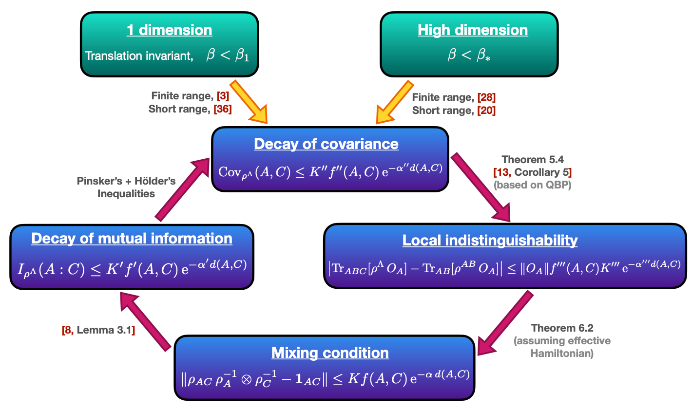
Figure 1: Summary of the main results contained in this paper. The equivalence between the four notions of decay of correlations is valid for short-range interactions. For one-dimensional spin systems, $\beta_{1}$ reduces to $\infty$ for finite-range interactions. We consider a function positive $f$ on finite sets that can possibly be different for each type of correlation decay.

The implications from mixing condition to decay of mutual information and subsequently to decay of covariance were already derived in [8, Lemma 3.1], where the latter quantity was shown to be upper bounded by the former. From decay of correlations to local indistinguishability, we recreate the steps of [8, Proposition 7.1] for the one-dimensional case in the current setting. We include here for completeness a self-contained, normalized and rigorous version of [25] for short-range interactions, and refer to [13] for its derivation in full detail.

1.3 Mixing condition and proof outline

The main result of this paper deals with the implication from local indistinguishability to mixing condition, and requires tools such as the construction of a local effective Hamiltonian and the so-called Quantum Belief Propagation (QBP) [23, 27, 26].

More specifically, we prove that, given a finite lattice $\Lambda\subset\mathbb{Z}^{g}$ and $A,C\subset\Lambda$ such that $A$ and $C$ are “separated enough”, and for a Gibbs state $\rho^{\Lambda}(\beta)\equiv\rho=\frac{\operatorname{e}^{-\beta H_{\Lambda}}}{\Tr[\operatorname{e}^{-\beta H_{\Lambda}}]}$ of a short-range Hamiltonian with $\beta<\beta_{*}$, where $\beta_{*}$ is some sufficiently low inverse temperature, we have

$$\norm{\rho_{AC}\,\rho_{A}^{-1}\otimes\rho_{C}^{-1}-\mathds{1}_{AC}}_{\infty}\leq\zeta\operatorname{e}^{-\eta\mathrm{dist}(A,C)}\,,$$

where $\zeta,\eta$ are absolute constants depending on the interactions and $\beta$, and additionally $\zeta=\mathcal{O}\left(e^{\operatorname{min}\{|\partial A|,|\partial B|,|\partial C|\}},\min\{f(A,C),f(C,A)\},e^{\beta}\right)$. Here, $\partial X$ is the $1$-boundary of $X$, i.e., all sites in the complement of $X$ that have distance $1$ from $X$.

The proof of this result is quite involved and requires the use of strong machinery in the context of Gibbs states. In particular, we make use in our proof of the so-called cluster expansions, the well-known Quantum Belief Propagation (QBP) and estimates on Araki’s expansionals. Let us sketch here the proof of this result by combining these tools. The complete proof can be found in the next sections.

Step 1. Construction of the effective Hamiltonian.

In a first step, following the ideas of [31], we construct a local effective Hamiltonian $\widetilde{H}^{L,\beta}_{\Lambda}$ from our original Hamiltonian $H_{\Lambda}$ such that, for every $L\subset\Lambda$ (cf. Section 3):

$$\widetilde{H}^{L,\beta}_{\Lambda}:=-\frac{1}{\beta}\log\left(\tr_{L^{c}}(e^{-\beta H_{\Lambda}})\otimes\mathbbm{1}_{L^{c}}\right)+\frac{1}{\beta}\log[Z_{L^{c}}]\mathbbm{1}\,.$$

We can control the interaction terms of $\operatorname{e}^{-\beta\widetilde{H}_{\Lambda}^{L,\beta}}$, as well as bound the expansionals of the form

$$\operatorname{e}^{-\beta\widetilde{H}_{\Lambda}^{AB,\beta}}\operatorname{e}^{\beta(\widetilde{H}_{\Lambda}^{A,\beta}+\widetilde{H}_{\Lambda}^{B,\beta})}\,.$$

In particular, the previous construction allows us to relate the marginals of the original Hamiltonian to the exponentials of the effective Hamiltonian in the following form (see Eq. (56)):

$$\rho_{AC}\,\rho_{A}^{-1}\otimes\rho_{C}^{-1}=\operatorname{e}^{-\beta\widetilde{H}_{\Lambda}^{AC,\beta}}\operatorname{e}^{\beta(\widetilde{H}_{\Lambda}^{A,\beta}+\widetilde{H}_{\Lambda}^{C,\beta})}\underbrace{Z_{ABC}Z_{B}Z_{AB}^{-1}Z_{BC}^{-1}}_{\lambda_{ABC}}\,,$$

where $Z_{X}$ is just $\Tr_{X}[\operatorname{e}^{-\beta H_{X}}]$. Therefore, we can bound

$$\norm{\rho_{AC}\rho_{A}^{-1}\otimes\rho_{C}^{-1}-\mathds{1}}_{\infty}$$

$$\hskip 56.9055pt\leq\norm{\operatorname{e}^{-\beta\widetilde{H}_{\Lambda}^{AC,\beta}}\operatorname{e}^{\beta(\widetilde{H}_{\Lambda}^{A,\beta}+\widetilde{H}_{\Lambda}^{C,\beta})}}_{\infty}\absolutevalue{\lambda_{ABC}-1}+\norm{\operatorname{e}^{-\beta\widetilde{H}_{\Lambda}^{AC,\beta}}\operatorname{e}^{\beta(\widetilde{H}_{\Lambda}^{A,\beta}+\widetilde{H}_{\Lambda}^{C,\beta})}-\mathds{1}_{AC}}_{\infty}\,.$$ (1)

Now we need to estimate each of these terms separately.

Step 2. Estimates on the expansionals of the effective Hamiltonian.

For estimating the last term in the RHS of Eq. (1.3), we use the estimates for Araki’s expansionals for the effective Hamiltonian from Lemma 4.1, concluding:

$$\norm{\operatorname{e}^{-\beta\widetilde{H}_{\Lambda}^{AC,\beta}}\operatorname{e}^{\beta(\widetilde{H}_{\Lambda}^{A,\beta}+\widetilde{H}_{\Lambda}^{C,\beta})}}_{\infty}\leq\operatorname{e}^{\mathcal{K}_{1}\mathcal{K}_{2}}\,,$$

for $\mathcal{K}_{1}$ a constant and

$$\mathcal{K}_{2}\leq\mathcal{O}\left({\operatorname{min}\{|\partial A|,|\partial C|\}}\operatorname{e}^{-\mathrm{dist}(A,C)}\right)\,.$$

We can similarly estimate the first term in the RHS above, as done in 4.2, obtaining:

$$\norm{\operatorname{e}^{-\beta\widetilde{H}_{\Lambda}^{AC,\beta}}\operatorname{e}^{\beta(\widetilde{H}_{\Lambda}^{A,\beta}+\widetilde{H}_{\Lambda}^{C,\beta})}-\mathds{1}_{AC}}_{\infty}\leq\operatorname{e}^{\mathcal{K}_{1}\mathcal{K}_{2}}-1\,.$$

Step 3. Estimates on partition functions of the original Hamiltonian.

The remaining term from Eq. (1.3) to be bounded is $\absolutevalue{\lambda_{ABC}-1}$. We bound it in 6.1 using the result of local indistinguishability from 5.4 as well as the estimates for Araki’s expansionals for the original Hamiltonian from 2.2, obtaining thus:

$$\absolutevalue{\lambda_{ABC}-1}\leq\min\{\mathcal{O}(|\partial A|+|C|g(A))e^{\mathcal{O}(|\partial A|)},\mathcal{O}(|\partial C|+|A|g(C))e^{\mathcal{O}(|\partial C|)}\}\,,$$

where the factors $g(A)$ and $g(C)$ are inherited from the notion of clustering of correlations assumed to hold. Note that, in the proof of 5.4, we additionally make use of the Quantum Belief Propagation.

2 Setting and beyond

2.1 Notations and model

Let $G=(V,E)$ be a possibly infinite graph with vertices $V$ and edges $E$. We endow the graph with a metric $\mathrm{dist}:V\times V\to\mathbb{R}_{+}$, for example the shortest path distance on the graph. This fixes the lattice $V$ our quantum systems live on. For the distance between sets $X$, $Y\subset V$, let

$$\mathrm{dist}(X,Y):=\inf_{x\in X}\inf_{y\in Y}\mathrm{dist}(x,y)\,.$$

We write the double inclusion $X\subset\subset V$ to indicate that the subset $X$ is finite. The set of finite subsets of $V$ will be denoted by $\mathcal{P}_{f}(V)$.

The diameter of a finite subset $X$ of $V$ is given by $\operatorname{diam}(X)=\max_{x,y\in X}\mathrm{dist}(x,y)$. Let us denote by $\Delta_{r}$ the maximum cardinal of a set of diameter less than or equal to $r$. Note that for $V=\mathbb{Z}^{g}$, $g\in\mathbb{N}$, and the Euclidean distance, we can estimate $\Delta_{r}\leq(2r+1)^{g}$. For $A\subset\subset V$, we denote by $\partial_{r}A$ the subset of $A$ made of all sites whose distance from $A^{c}:=V\setminus A$ is less than or equal to $r$. In particular, we will write $\partial A:=\partial_{1}A$.

Let us now come to the Hilbert space associated to the quantum spin system. At each lattice site $x\in V$ we set a local Hilbert space $\mathcal{H}_{x}\equiv\mathbb{C}^{D}$ of dimension $D\in\mathbb{N}$. For each $X\in\mathcal{P}_{f}(V)$ we then have the space of states $\mathcal{H}_{X}=\otimes_{v\in X}\mathcal{H}_{v}\equiv(\mathbb{C}^{D})^{\otimes|X|}$ of dimension $D_{X}=D^{|X|}$ and the algebra of observables $\mathfrak{A}_{X}=\mathcal{B}(\mathcal{H}_{X})$. As usual, for two finite subsets $X$, $Y$ of $V$ such that $X\subset Y$ we identify $\mathfrak{A}_{X}\subset\mathfrak{A}_{Y}$ via the canonical linear isometry $\mathfrak{A}_{X}\to\mathfrak{A}_{Y}$ given by $Q\mapsto Q\otimes\mathbbm{1}_{Y\setminus X}$.

Next, we will describe which notation we will use for different versions of the trace. For each $X\in\mathcal{P}_{f}(V)$, we will denote by $\Tr_{X}:\mathfrak{A}_{X}\longrightarrow\mathbb{C}$ the full (unnormalized) trace over $X$. For the partial trace over $X$ on any $\mathcal{P}_{f}(V)\ni X^{\prime}\supset X$ we will write

$$\operatorname{tr}_{X}:=\mathrm{Tr}_{X}\otimes\mathrm{id}_{X^{\prime}\setminus X}:\mathfrak{A}_{X^{\prime}}\longrightarrow\mathfrak{A}_{X^{\prime}\setminus X}$$

and combine this map with the above canonical isometries. For instance, for a state $\sigma\in\mathfrak{A}_{X^{\prime}}$ and $X\subset X^{\prime}$, we can write $\operatorname{tr}_{X}(\sigma)=\operatorname{tr}_{X}(\sigma)\otimes\mathds{1}_{X}\in\mathfrak{A}_{X^{\prime}}$. In particular, if $Q\in\mathfrak{A}_{X}$, then we will deal with $\operatorname{tr}_{X}(Q)$ as a multiple of identity, $\operatorname{tr}_{X}(Q)=\Tr_{X}(Q)\mathds{1}_{X}$. The normalized version of the partial trace, which is a conditional expectation, will be denoted $\mathbb{E}_{X^{c}}:=\tr_{X}/D_{X}$. In this case, given $Q\in\mathfrak{A}_{X}$ and $\mathcal{P}_{f}(V)\ni Y,Y^{\prime}\supset X$ we can identify $\mathbb{E}_{Y^{c}}(Q)=\mathbb{E}_{(Y^{\prime})^{c}}(Q)$.

In terms of norms, we will denote by $\|Q\|_{\infty}$ or simply $\|Q\|$ the operator norm of $Q\in\mathfrak{A}_{X}$, and by $\|Q\|_{1}=\operatorname{Tr}_{X}(|Q|)$ its trace norm.

Let us present now the kind of Hamiltonians we will consider. By a local interaction, we refer to a family $\Phi=(\Phi_{X})_{X\in\mathcal{P}_{f}(V)}$, where $\Phi_{X}\in\mathfrak{A}_{X}$ and $\Phi_{X}=\Phi_{X}^{\ast}$ for every $X\in\mathcal{P}_{f}(V)$. To quantify the decay of the interactions, we introduce for each $\lambda,\mu>0$ the following notation

$$\|\Phi\|_{\lambda,\mu}:=\sup_{x\in V}\sum_{X\ni x}\|\Phi_{X}\|e^{\lambda|X|+\mu\operatorname{diam}(X)}\in[0,\infty]\,.$$ (2)

We will say that $\Phi$ has finite range $r>0$ and strength $J>0$ if $\|\Phi_{X}\|=0$ whenever $X$ has diameter greater than $r$ and $\|\Phi_{X}\|\leq J$ for all $X\in\mathcal{P}_{f}(V)$. Moreover, we will say that $\Phi$ has short range, or it is exponentially decaying, if $\norm{\Phi}_{\lambda,\mu}<\infty$. As usual, we denote for every finite subset $Y\subset\subset V$ the corresponding Hamiltonian by

$$H_{Y}:=\sum_{X\subset Y}{\Phi_{X}}\,,$$

the time-evolution operator (with possibly complex-valued time) by

$$\Gamma^{s}_{H_{Y}}(Q)=e^{isH_{Y}}Qe^{-isH_{Y}}\quad,\quad s\in\mathbb{C}\,,$$

and the Gibbs state at inverse temperature $\beta>0$ by

$$\rho^{Y}_{\beta}:=\frac{e^{-\beta H_{Y}}}{\Tr_{Y}[e^{-\beta H_{Y}}]}\,.$$

Moreover, for any $X\subset Y$, we denote by $\rho_{\beta,X}^{Y}$ the marginal in $X$ of the Gibbs state of $H_{Y}$ at inverse temperature $\beta>0$, namely

$$\rho_{\beta,X}^{Y}:=\tr_{Y\setminus X}\left[\rho^{Y}_{\beta}\right]\,.$$

Note that seen as an element in $\mathfrak{A}_{Y}$, $\rho_{\beta,X}^{Y}$ is no longer a quantum state, because its trace is no longer normalized. We will frequently drop the superindex $Y$ when it is clear from the context, as well as the subindex $\beta$ when we are fixing the temperature.

2.2 Locality and time evolution

We devote this subsection to deriving some estimates on the norm of the time-evolution operator for short-range interactions. We provide below both universal estimates on such time-evolution operators, as well as decay estimates on the difference between pairs of them.

Proposition 2.1.

Let $\Phi$ be an interaction on $V$ (not necessarily with finite range) such that for some positive constants $\lambda,\mu$ and $g_{\lambda,\mu}$ the following condition holds

$$\sup_{x\in V}\sum_{X\ni x}\|\Phi_{X}\|e^{\lambda|X|+\mu\operatorname{diam}(X)}\leq g_{\lambda,\mu}\,,$$ (3)

and let $Q$ be an observable having support in a finite subset $Z$ of $V$. Then, for every $s\in\mathbb{C}$ with $|s|<\lambda/(2g_{\lambda,\mu})$ it holds that

$$\|\Gamma_{\Phi}^{s}(Q)\|\leq\|Q\|\,e^{\lambda|Z|}\,\frac{\lambda}{\lambda-2g_{\lambda,\mu}|s|}\,.$$ (4)

Moreover, let $Y$ be any finite subset of $V$ with $Z\subset Y$ and let $\Phi^{Y}$ be the interaction given by $\Phi^{Y}_{X}=\Phi_{X}$ for every $X\subset Y$ and $\Phi^{Y}_{X}=0$ if $X\cap Y^{c}\neq\emptyset$ (we can interpret $\Phi^{Y}$ as the restriction of the interaction $\Phi$ to $Y$). Then, for every $s\in\mathbb{C}$ with $|s|<\lambda/(2g_{\lambda,\mu})$,

$$\left\|\Gamma_{\Phi}^{s}(Q)-\Gamma_{\Phi^{Y}}^{s}(Q)\right\|\leq\|Q\|\,e^{\lambda|Z|}\,\frac{2g_{\lambda,\mu}|s|\lambda}{(\lambda-2g_{\lambda,\mu}|s|)^{2}}\,e^{-\mu\operatorname{dist}(Z,Y^{c})}\,.$$ (5)

Before proving this result, let us mention that Eq. (4) should be compared to [10, Theorem 6.2.4], to which our estimate reduces whenever $\mu=0$. Moreover, Eq. (5) for $\mu=0$ is essentially in [10, after Theorem 6.2.4] and can be interpreted in a sense as a property of locality of the interactions. Note that we have introduced the weight $e^{\mu\operatorname{diam}(X)}$ to control the decay of the interactions with the diameter, following the lines of [37].

Proof.

The time evolution operator is defined in terms of the derivation operator $\delta_{H}(Q)=i[H,Q]$ as

$$\Gamma_{\Phi}^{s}(Q)=\sum_{m=0}^{\infty}\frac{s^{m}}{m!}b_{\Phi}^{m}(Q)\,.$$ (6)

where

$$b_{\Phi}^{m}(Q)=\sum_{X_{1}\cap Z\neq\emptyset}\ldots\sum_{X_{m}\cap S_{m-1}\neq\emptyset}\,\delta_{X_{m}}\circ\delta_{X_{m-1}}\circ\ldots\circ\delta_{X_{1}}(Q)\,,$$

and $S_{0}:=Z$, $S_{j}:=Z\cup X_{1}\cup\ldots\cup X_{j}$ for $1\leq j\leq m$. We next follow an argument inspired by the proof of [10, Theorem 6.2.4] to estimate

$$\|b_{\Phi}^{m}(Q)\|\leq 2^{m}\|Q\|\sum_{X_{1}\cap Z\neq\emptyset}\ldots\sum_{X_{m}\cap S_{m-1}\neq\emptyset}\,\,\,\prod_{j=1}^{m}\|\Phi_{X_{j}}\|\,.$$ (7)

Next, let us rewrite

$$\prod_{j=1}^{m}\|\Phi_{X_{j}}\|=e^{-\lambda(|X_{1}|+\ldots|X_{m}|)}\,\prod_{j=1}^{m}\|\Phi_{X_{j}}\|e^{\lambda|X_{j}|}\leq e^{\lambda|Z|}e^{-\lambda|S_{m}|}\,\prod_{j=1}^{m}\|\Phi_{X_{j}}\|e^{\lambda|X_{j}|}\,.$$

Applying the inequality $e^{-\lambda x}\leq\frac{m!}{\lambda^{m}x^{m}}$ with $x=|S_{m}|$ in the previous expression, we moreover get

$$\prod_{j=1}^{m}\|\Phi_{X_{j}}\|\leq e^{\lambda|Z|}\frac{m!}{|S_{m}|^{m}\lambda^{m}}\,\prod_{j=1}^{m}\|\Phi_{X_{j}}\|e^{\lambda|X_{j}|}\leq e^{\lambda|Z|}\frac{m!}{\lambda^{m}}\,\prod_{j=1}^{m}\frac{1}{|S_{j-1}|}\|\Phi_{X_{j}}\|e^{\lambda|X_{j}|}\,,$$ (8)

and thus

$$\|b_{\Phi}^{m}(Q)\|\leq 2^{m}\|Q\|\,e^{\lambda|Z|}\frac{m!}{\lambda^{m}}\sum_{X_{1}\cap Z\neq\emptyset}\ldots\sum_{X_{m}\cap S_{m-1}\neq\emptyset}\,\,\,\prod_{j=1}^{m}\frac{1}{|S_{j-1}|}\|\Phi_{X_{j}}\|e^{\lambda|X_{j}|}\,.$$ (9)

Finally, note that we can bound for each finite subset $Y$ of the lattice

$$\sum_{X\cap Y\neq\emptyset}\|\Phi_{X}\|e^{\lambda|X|+\mu\operatorname{diam}(X)}\leq\sum_{v\in Y}\sum_{X\ni v}\|\Phi_{X}\|e^{\lambda|X|+\mu\operatorname{diam}(X)}\leq|Y|g_{\lambda,\mu}\,.$$ (10)

Applying Eq. (10) iteratively, we can estimate

$$\sum_{X_{1}\cap Z\neq\emptyset}\ldots\sum_{X_{m}\cap S_{m-1}\neq\emptyset}\,\,\,\prod_{j=1}^{m}\frac{1}{|S_{j-1}|}\|\Phi_{X_{j}}\|e^{\lambda|X_{j}|}\leq g_{\lambda,\mu}^{m}\,,$$

such that

$$\|b_{\Phi}^{m}(Q)\|\leq\left(\frac{2g_{\lambda,\mu}}{\lambda}\right)^{m}\|Q\|\,e^{\lambda|Z|}\,m!\,.$$ (11)

Replacing Eq. (11) in Eq. (6),

$$\|\Gamma_{\Phi}^{s}(Q)\|\leq\|Q\|\,e^{\lambda|Z|}\,\sum_{m=0}^{\infty}\left(\frac{2g_{\lambda,\mu}|s|}{\lambda}\right)^{m}\,.$$

Using finally the formula $\frac{1}{1-x}=\sum_{m=0}^{\infty}x^{m}$ for $|x|<1$ we arrive at Eq. (3).

Next, we prove the other estimate. Using Eq. (6), we can again upper bound

$$\|\Gamma^{s}_{\Phi}(Q)-\Gamma^{s}_{\Phi^{Y}}(Q)\|\leq\sum_{m=1}^{\infty}\frac{|s|^{m}}{m!}\left\|b_{\Phi}^{m}(Q)-b_{\Phi^{Y}}^{m}(Q)\right\|\,.$$ (12)

Each summand can be bounded following a similar strategy to the first inequality of the theorem. First, let

$$\|b_{\Phi}^{m}(Q)-b_{\Phi^{Y}}^{m}(Q)\|\\ \leq 2^{m}\|Q\|\sum_{j=1}^{m}\sum_{X_{1}\cap Z\neq\emptyset}\ldots\sum_{X_{m}\cap S_{m-1}\neq\emptyset}\left(\prod_{\begin{subarray}{c}i=1\end{subarray}}^{j-1}\|\Phi^{Y}_{X_{i}}\|\right)\cdot\|\Phi_{X_{j}}-\Phi^{Y}_{X_{j}}\|\cdot\left(\prod_{\begin{subarray}{c}i=j+1\end{subarray}}^{m}\|\Phi_{X_{i}}\|\right)\,.$$ (13)

To deal with the previous term, we argue as with Eq. (7), but adding one additional intermediate step. More specifically, we first estimate as in Eq. (8) to get for each $j\in\{1,\ldots,m\}$

$$\begin{split}&\left(\prod_{\begin{subarray}{c}i=1\end{subarray}}^{j-1}\|\Phi^{Y}_{X_{i}}\|\right)\cdot\|\Phi^{Y}_{X_{j}}-\Phi_{X_{j}}\|\cdot\left(\prod_{\begin{subarray}{c}i=j+1\end{subarray}}^{m}\|\Phi_{X_{i}}\|\right)\leq\\[5.69054pt] &\hskip 85.35826pt\leq e^{\lambda|Z|}\frac{m!}{\lambda^{m}}\,\,\left(\prod_{\begin{subarray}{c}i=1\end{subarray}}^{j-1}\frac{\|\Phi^{Y}_{X_{i}}\|e^{\lambda|X_{i}|}}{|S_{i-1}|}\right)\cdot\frac{\|\Phi^{Y}_{X_{j}}-\Phi_{X_{j}}\|e^{\lambda|X_{j}|}}{|S_{j-1}|}\cdot\left(\prod_{\begin{subarray}{c}i=j+1\end{subarray}}^{m}\frac{\|\Phi_{X_{i}}\|e^{\lambda|X_{i}|}}{|S_{i-1}|}\right)\,.\end{split}$$

Then, applying Eq. (10) to the last $m-j$ terms iteratively

$$\begin{split}&\sum_{X_{1}\cap Z\neq\emptyset}\ldots\sum_{X_{m}\cap S_{m-1}\neq\emptyset}\left(\prod_{\begin{subarray}{c}i=1\end{subarray}}^{j-1}\|\Phi^{Y}_{X_{i}}\|\right)\cdot\|\Phi^{Y}_{X_{j}}-\Phi_{X_{j}}\|\cdot\left(\prod_{\begin{subarray}{c}i=j+1\end{subarray}}^{m}\|\Phi_{X_{i}}\|\right)\\[5.69054pt] &\hskip 28.45274pt\leq g_{\lambda,\mu}^{m-j}\cdot e^{\lambda|Z|}\frac{m!}{\lambda^{m}}\sum_{X_{1}\cap Z\neq\emptyset}\ldots\sum_{X_{j}\cap S_{j-1}\neq\emptyset}\left(\prod_{\begin{subarray}{c}i=1\end{subarray}}^{j-1}\frac{\|\Phi^{Y}_{X_{i}}\|e^{\lambda|X_{i}|}}{|S_{i-1}|}\right)\cdot\frac{\|\Phi^{Y}_{X_{j}}-\Phi_{X_{j}}\|e^{\lambda|X_{j}|}}{|S_{j-1}|}\,.\end{split}$$ (14)

Let us observe that, by definition, $\Phi_{X}-\Phi_{X}^{Y}=0$ if $X\subset Y$ and $\Phi_{X}-\Phi_{X}^{Y}=\Phi_{X}$ if $X\nsubseteq Y$ (i.e. $X\cap(V\setminus Y)\neq\emptyset$). Thus, in the above expression we can restrict the sum over $X_{j}$ with $X_{j}\cap S_{j-1}\neq\emptyset$ to sets $X_{j}$ that also satisfy $X_{j}\cap(V\setminus Y)\neq\emptyset$ and simplify $\Phi_{X_{j}}-\Phi_{X_{j}}^{Y}=\Phi_{X}$. Thus, the upper bound from Eq. (14) can be rewritten as

$$g_{\lambda,\mu}^{m-j}\cdot e^{\lambda|Z|}\frac{m!}{\lambda^{m}}\sum_{X_{1}\cap Z\neq\emptyset}\ldots\sum_{X_{j-1}\cap S_{j-2}\neq\emptyset}\sum_{\begin{subarray}{c}X_{j}\cap S_{j-1}\neq\emptyset\\ X_{j}\cap(V\setminus Y)\neq\emptyset\end{subarray}}\left(\prod_{\begin{subarray}{c}i=1\end{subarray}}^{j-1}\frac{\|\Phi^{Y}_{X_{i}}\|e^{\lambda|X_{i}|}}{|S_{i-1}|}\right)\cdot\frac{\|\Phi_{X_{j}}\|e^{\lambda|X_{j}|}}{|S_{j-1}|}\,.$$ (15)

Note that the conditions on $X_{1},\ldots,X_{j}$ yield that

$$\operatorname{dist}(Z,V\setminus Y)\leq\sum_{i=1}^{j}\operatorname{diam}(X_{i})\,.$$

Hence, we can introduce a factor:

$$\left(\prod_{\begin{subarray}{c}i=1\end{subarray}}^{j-1}\frac{\|\Phi^{Y}_{X_{i}}\|e^{\lambda|X_{i}|}}{|S_{i-1}|}\right)\cdot\frac{\|\Phi_{X_{j}}\|e^{\lambda|X_{j}|}}{|S_{j-1}|}\\ \leq\left(\prod_{\begin{subarray}{c}i=1\end{subarray}}^{j-1}\frac{\|\Phi^{Y}_{X_{i}}\|e^{\lambda|X_{i}|+\mu\operatorname{diam}(X_{i})}}{|S_{i-1}|}\right)\cdot\frac{\|\Phi_{X_{j}}\|e^{\lambda|X_{j}|+\mu\operatorname{diam}(X_{j})}}{|S_{j-1}|}e^{-\mu\operatorname{dist}(Z,V\setminus Y)}\,.$$ (16)

Inserting the last expression in Eq.  (15), and using again Eq. (10) to show that

$$\sum_{X_{1}\cap Z\neq\emptyset}\ldots\sum_{X_{j-1}\cap S_{j-2}\neq\emptyset}\sum_{X_{j}\cap S_{j-1}\neq\emptyset}\left(\prod_{\begin{subarray}{c}i=1\end{subarray}}^{j-1}\frac{\|\Phi^{Y}_{X_{i}}\|e^{\lambda|X_{i}|+\mu\operatorname{diam}(X_{i})}}{|S_{i-1}|}\right)\cdot\frac{\|\Phi_{X_{j}}\|e^{\lambda|X_{j}|+\mu\operatorname{diam}(X_{j})}}{|S_{j-1}|}\leq g_{\lambda,\mu}^{j}\,,$$

we conclude from Eq. (13)

$$\|b_{\Phi}^{m}(Q)-b_{\Phi^{\prime}}^{m}(Q)\| \leq 2^{m}\|Q\|m\,\frac{m!}{\lambda^{m}}\,g_{\lambda,\mu}^{m}\,e^{\lambda|Z|}\,e^{-\mu\operatorname{dist}(Z,V\setminus Y)}\,.$$

Replacing this estimate in Eq. (12), we conclude that

$$\left\|\Gamma_{\Phi}^{s}(Q)-\Gamma_{\Phi^{\prime}}^{s}(Q)\right\|\leq\|Q\|\,e^{\lambda|Z|}\,\sum_{m=1}^{\infty}m\left(\frac{2g_{\lambda,\mu}|s|}{\lambda}\right)^{m}e^{-\mu\operatorname{dist}(Z,V\setminus Y)}\,.$$

Finally, we apply the formula $x/(1-x)^{2}=\sum_{m=1}^{\infty}mx^{m}$ with $x=2g_{\lambda,\mu}|s|/\lambda<1$ to get the desired result. ∎

2.3 Araki’s expansionals

In this subsection, we present some estimates on Araki’s expansionals [3] for a Hamiltonian with short-range interactions. We use the following notation for the expansionals:

$$E_{X,Y}(s):= \operatorname{e}^{-sH_{XY}}\operatorname{e}^{sH_{X}+sH_{Y}}\,\quad\text{ for every }s\in\mathbb{C}\,.$$

$$E_{X,Y}:= E_{X,Y}(1)=\operatorname{e}^{-H_{XY}}\operatorname{e}^{H_{X}+H_{Y}}\,.$$

First let us recall that for every pair of observables $H$ and $W$ and every real value $\beta\geq 0$ we have the following expansion in terms of the time-evolution operator (see [3, Eq. (5.1)])

$$e^{\beta(H+W)}e^{-\beta H}=\sum_{m=0}^{\infty}\,\,\int_{0}^{\beta}dt_{1}\int_{0}^{t_{1}}dt_{2}\ldots\int_{0}^{t_{m-1}}dt_{m}\,\,\prod_{j}^{m\to 1}\Gamma_{H}^{-it_{j}}(W)\,,$$

where we are denoting $\underset{j}{\overset{m\to n}{\prod}}Q_{j}:=Q_{m}Q_{m-1}\ldots Q_{n}$ for every $m\geq n$, and where we recall that $\Gamma_{H}^{it}(W)=e^{tH}We^{-tH}$. Changing the signs $H\mapsto-H$ and $W\mapsto-W$ we can then rewrite

$$e^{-\beta(H+W)}e^{\beta H}=\sum_{m=0}^{\infty}(-1)^{m}\,\,\int_{0}^{\beta}dt_{1}\int_{0}^{t_{1}}dt_{2}\ldots\int_{0}^{t_{m-1}}dt_{m}\,\,\prod_{j}^{m\to 1}\Gamma_{H}^{it_{j}}(W)\,.$$ (17)

Proposition 2.2.

Let $A,B,C$ be disjoint finite subsets of $V$ and let $\Phi$ be a local interaction on $V$ satisfying Eq. (3) for $\lambda,\mu,g_{\lambda,\mu}>0$. Then, for every real number $\beta$ with $|\beta|<\frac{\lambda}{2g_{\lambda,\mu}}$ we have

$$\norm{E_{A,B}(\beta)}\leq\exp{\frac{g_{\lambda,\mu}|\beta|\lambda}{\lambda-2g_{\lambda,\mu}|\beta|}\,\textstyle\sum_{v\in A}e^{-\mu\operatorname{dist}(v,B)}}\,,$$ (18)

and

$$\norm{E_{A,BC}(\beta)-E_{A,B}(\beta)}\leq\exp{\frac{g_{\lambda,\mu}|\beta|\lambda}{\lambda-2g_{\lambda,\mu}|\beta|}\sum_{v\in A}e^{-\mu\operatorname{dist}(v,BC)}}\cdot\frac{|\beta|g_{\lambda,\mu}^{2}(\lambda+|\beta|)^{2}}{(\lambda-2g_{\lambda,\mu}|\beta|)^{2}}\sum_{v\in A}e^{-\mu\operatorname{dist}(v,C)}\,.$$ (19)

Remark 2.3.

In fact, the exponential growth in $\beta$ is unavoidable, as one can see from the commutative case.

Remark 2.4.

We can estimate for example

$$\sum_{v\in A}e^{-\mu\operatorname{dist}(v,X)}\leq\sum_{k=0}^{\infty}|\{x\in A\colon k<\operatorname{dist}(x,X)\leq k+1\}|e^{-\mu k}\,.$$

Let us make the following assumption:

Assumption 2.5.

Let $(V,\operatorname{dist})$ be such that there exist constants $\nu_{1}$, $\nu_{2}>0$ such that

$$\sup_{x}\mathcal{B}_{\ell}(x)\leq\nu_{1}\ell^{\nu_{2}}\,.$$

Then, we have

$$\sup_{k\geq 0}|\{x\in A\colon k<\operatorname{dist}(x,A^{c})\leq k+1\}|\leq\nu_{1}|\partial A|(k+1)^{\nu_{2}}$$

and there is a constant $\nu=:\nu_{1}\sup_{k\in\mathbb{N}}(k+1)^{\nu_{2}}e^{-\mu/2k}$ such that

$$\sum_{v\in A}e^{-\mu\operatorname{dist}(v,X)}\leq\nu|\partial A|\sum_{k\geq\lfloor\mathrm{dist}(A,X)\rfloor}e^{-\frac{\mu}{2}k}\,.$$

Note that by 2.4, assuming that $B$ shields $A$ from $C$, we can simplify the estimates in Eq. (18) by

$$\norm{E_{A,B}(\beta)}\leq\exp\{|\beta|\min\{|\partial A|,|\partial B|\}K_{\mu,\lambda}\}\,,$$ (20)

and

$$\norm{E_{A,BC}(\beta)-E_{A,B}(\beta)}$$

$$\hskip 28.45274pt\leq C_{\mu,\lambda}\exp\{|\beta|\min\{|\partial A|,|\partial_{A}B|\}K_{\mu,\lambda}\}\min\{|\partial A|,|\partial C|\}\exp\{-\hat{K}_{\mu,\lambda}\operatorname{dist}(A,C)\}\,,$$ (21)

for certain constants $C_{\mu,\lambda},K_{\mu,\lambda},\hat{K}_{\mu,\lambda}>0$ depending only on $d,\mu$ and $\lambda$, and denoting by $\partial_{A}B$ the boundary of $B$ contained in $A$.

Proof of 2.2.

Let us start with the following observation: We can restrict the proof of the theorem to values $\beta\geq 0$, since for values $\beta<0$ we can rewrite

$$E_{X,Y}(\beta)=e^{-|\beta|\hat{H}_{XY}}e^{|\beta|\hat{H}_{X}+|\beta|\hat{H}_{Y}}\,,$$

where $\hat{H}$ is the Hamiltonian associated to the interaction by changing the local interaction $\hat{\Phi}=-\Phi$, which satisfies the same bound Eq. (3) for $\lambda,\mu,g_{\lambda,\mu}>0$. Let us start with an observation that will be useful at several points of the proof. For an arbitrary pair of disjoint subsets $A$,$B\in\mathcal{P}_{f}(V)$ we can estimate

$$\underset{\tiny{\begin{array}[]{c}Z\subset V\\ Z\cap A\neq\emptyset\\ Z\cap B\neq\emptyset\end{array}}}{\sum}\norm{\Phi_{Z}}\operatorname{e}^{\lambda\absolutevalue{Z}} \leq\sum_{v\in A}\underset{\tiny{\begin{array}[]{c}Z\ni v\\ Z\cap B\neq\emptyset\end{array}}}{\sum}\norm{\Phi_{Z}}\operatorname{e}^{\lambda\absolutevalue{Z}}$$ (27)

$$=\sum_{v\in A}\underset{\tiny{\begin{array}[]{c}Z\ni v\\ Z\cap B\neq\emptyset\end{array}}}{\sum}\norm{\Phi_{Z}}\operatorname{e}^{\lambda\absolutevalue{Z}}\operatorname{e}^{\mu\,\text{diam}(Z)}\operatorname{e}^{-\mu\,\text{diam}(Z)}$$ (30)

$$\leq\sum_{v\in A}\underset{\tiny{\begin{array}[]{c}Z\ni v\\ Z\cap B\neq\emptyset\end{array}}}{\sum}\norm{\Phi_{Z}}\operatorname{e}^{\lambda\absolutevalue{Z}}\operatorname{e}^{\mu\,\text{diam}(Z)}\operatorname{e}^{-\mu\,\text{dist}(v,B)}$$ (33)

$$\leq g_{\lambda,\mu}\sum_{v\in A}e^{-\mu\operatorname{dist}(v,B)}$$ (34)

To prove Eq. (18), let us consider $H\equiv H_{A}+H_{B}$ and $W\equiv W_{A,B}=H_{AB}-H_{A}-H_{B}$ in Eq. (17), yielding for every $\beta\in\mathbb{R}$:

$$E_{A,B}(\beta) =\sum_{m=0}^{\infty}(-1)^{m}\,\,\int_{0}^{\beta}dt_{1}\int_{0}^{t_{1}}dt_{2}\ldots\int_{0}^{t_{m-1}}dt_{m}\,\,\prod_{j}^{m\to 1}\Gamma_{H_{A}+H_{B}}^{it_{j}}(W_{A,B})\,,$$

Therefore, we can estimate

$$\left\|E_{A,B}(\beta)\right\|\leq 1+\sum_{m=1}^{\infty}\frac{\beta^{m}}{m!}\,\left(\sup_{0\leq\absolutevalue{t}\leq|\beta|}\|\Gamma^{it}_{H_{A}+H_{B}}(W_{A,B})\|\right)^{m}\,.$$ (35)

Now, let us recall that

$$\Gamma^{it}_{H_{A}+H_{B}}(W_{A,B})=\underset{\tiny{\begin{array}[]{c}Z\subset AB\\ Z\cap A\neq\emptyset\\ Z\cap B\neq\emptyset\end{array}}}{\sum}\Gamma^{it}_{H_{A}+H_{B}}(\Phi_{Z})\,.$$ (36)

Therefore,

$$\norm{\Gamma^{it}_{H_{A}+H_{B}}(W_{A,B})} \leq\underset{\tiny{\begin{array}[]{c}Z\subset AB\\ Z\cap A\neq\emptyset\\ Z\cap B\neq\emptyset\end{array}}}{\sum}\norm{\Gamma^{it}_{H_{A}+H_{B}}(\Phi_{Z})}$$

$$\leq\frac{\lambda}{\lambda-2g_{\lambda,\mu}|\beta|}\underset{\tiny{\begin{array}[]{c}Z\subset AB\\ Z\cap A\neq\emptyset\\ Z\cap B\neq\emptyset\end{array}}}{\sum}\norm{\Phi_{Z}}\operatorname{e}^{\lambda\absolutevalue{Z}}\,.$$

where we are using Proposition 2.1 in the second inequality. At this point, we can make use of the observation Eq. (34) to obtain the upper bound

$$\norm{\Gamma^{it}_{H_{A}+H_{B}}(W_{A,B})}\leq\frac{\lambda g_{\lambda,\mu}}{\lambda-2g_{\lambda,\mu}|\beta|}\,\sum_{v\in A}e^{-\mu\operatorname{dist}(v,B)}\,.$$ (37)

Finally, applying this upper estimate to Eq. (35), we conclude that Eq.  (18) holds.

Let us prove now Eq. (19) following similar ideas. First, note that

$$E_{A,B}(\beta)-E_{A,BC}(\beta)=\operatorname{e}^{-\beta H_{AB}}\operatorname{e}^{\beta H_{A}+\beta H_{B}}-\operatorname{e}^{-\beta H_{ABC}}\operatorname{e}^{\beta H_{A}+\beta H_{BC}}$$

$$=\sum_{m=1}^{\infty}\,\,\int_{0}^{\beta}dt_{1}\int_{0}^{t_{1}}dt_{2}\ldots\int_{0}^{t_{m-1}}dt_{m}\,\,\left[\underset{j}{\overset{m\to 1}{\prod}}\Gamma_{H_{A}+H_{B}}^{it_{j}}(W_{A,B})-\underset{j}{\overset{m\to 1}{\prod}}\Gamma_{H_{A}+H_{BC}}^{it_{j}}(W_{A,BC})\right]$$

Then,

$$\norm{E_{A,B}(\beta)-E_{A,BC}(\beta)}\leq\sum_{m=1}^{\infty}\frac{|\beta|^{m}}{m!}\underset{|t_{m}|,\ldots,|t_{1}|\leq|\beta|}{\text{sup}}\norm{\underset{j}{\overset{m\to 1}{\prod}}\Gamma_{H_{A}+H_{B}}^{it_{j}}(W_{A,B})-\underset{j}{\overset{m\to 1}{\prod}}\Gamma_{H_{A}+H_{BC}}^{it_{j}}(W_{A,BC})}\,.$$ (38)

Moreover, note that

$$\norm{\underset{j}{\overset{m\to 1}{\prod}}\Gamma_{H_{A}+H_{B}}^{it_{j}}(W_{A,B})-\underset{j}{\overset{m\to 1}{\prod}}\Gamma_{H_{A}+H_{BC}}^{it_{j}}(W_{A,BC})}$$

$$=\norm{\underset{\alpha=1}{\overset{m}{\sum}}\,\underset{j}{\overset{m\to(\alpha+1)}{\prod}}\Gamma_{H_{A}+H_{B}}^{it_{j}}(W_{A,B})\left(\Gamma_{H_{A}+H_{B}}^{it_{\alpha}}(W_{A,B})-\Gamma_{H_{A}+H_{BC}}^{it_{\alpha}}(W_{A,BC})\right)\underset{j}{\overset{(\alpha-1)\to 1}{\prod}}\Gamma_{H_{A}+H_{BC}}^{it_{j}}(W_{A,BC})}$$

$$\leq\sum_{\alpha=1}^{m}\underbrace{\norm{\Gamma_{H_{A}+H_{B}}^{it_{\alpha}}(W_{A,B})-\Gamma_{H_{A}+H_{BC}}^{it_{\alpha}}(W_{A,BC})}}_{(I)}\prod_{j=\alpha+1}^{m}\underbrace{\norm{\Gamma_{H_{A}+H_{B}}^{it_{j}}(W_{A,B})}}_{(II)}\prod_{j=1}^{\alpha-1}\underbrace{\norm{\Gamma_{H_{A}+H_{BC}}^{it_{j}}(W_{A,BC})}}_{(III)}\,.$$

We have classified the factors on the previous expression into three types (I), (II) and (III). Factors of type (II) can be upper estimate using Eq. (37). The same estimate can be applied to factors of type (III) adapted to the pair $A$ and $BC$ instead of $A$ and $B$. But since $\operatorname{dist}(v,B)\geq\operatorname{dist}(v,BC)$ for every $v\in A$, we can actually use the following common upper bound for both type of factors:

$$\norm{\Gamma_{H_{A}+H_{B}}^{it}(W_{A,B})},\norm{\Gamma_{H_{A}+H_{BC}}^{it}(W_{A,BC})}\leq\frac{\lambda g_{\lambda,\mu}}{\lambda-2g_{\lambda,\mu}|\beta|}\sum_{v\in A}e^{-\mu\operatorname{dist}(v,BC)}$$ (39)

To deal with the factor of type (I), let us split

$$\norm{\Gamma_{H_{A}+H_{B}}^{it}(W_{A,B})-\Gamma_{H_{A}+H_{BC}}^{it}(W_{A,BC})}$$

$$\leq\underbrace{\underset{\tiny{\begin{array}[]{c}Z\subset AB\\ Z\cap A\neq\emptyset\\ Z\cap B\neq\emptyset\end{array}}}{\sum}\norm{\Gamma_{H_{A}+H_{B}}^{it}(\Phi_{Z})-\Gamma_{H_{A}+H_{BC}}^{it}(\Phi_{Z})}}_{(III.1)}+\underbrace{\underset{\tiny{\begin{array}[]{c}Z\subset ABC\\ Z\cap A\neq\emptyset\\ Z\cap C\neq\emptyset\end{array}}}{\sum}\norm{\Gamma_{H_{A}+H_{BC}}^{it}(\Phi_{Z})}}_{(III.2)}\,.$$

For the second sum (III.2), we again use

$$\underset{\tiny{\begin{array}[]{c}Z\subset ABC\\ Z\cap A\neq\emptyset\\ Z\cap C\neq\emptyset\end{array}}}{\sum}\norm{\Gamma^{it}_{H_{A}+H_{BC}}(\Phi_{Z})} \leq\frac{\lambda g_{\lambda,\mu}}{\lambda-2g_{\lambda,\mu}|\beta|}\underset{\tiny{\begin{array}[]{c}Z\subset ABC\\ Z\cap A\neq\emptyset\\ Z\cap C\neq\emptyset\end{array}}}{\sum}\norm{\Phi_{Z}}e^{\lambda|Z|}$$ (46)

$$\leq\frac{\lambda g_{\lambda,\mu}^{2}}{\lambda-2g_{\lambda,\mu}|\beta|}\sum_{v\in A}e^{-\mu\operatorname{dist}(v,C)}\,,$$ (47)

where in the last inequality we have again used Eq. (34) for the pair $A$ and $C$. For the first sum (III.1), however, we are going to use inequality Eq. (5) from Proposition 2.1 with the interactions $\Phi^{A,B}$ and $\Phi^{A,BC}$ on $V=ABC$ giving $H_{A}+H_{B}$ and $H_{A}+H_{BC}$, respectively, and $Y=AB$:

$$\underset{\tiny{\begin{array}[]{c}Z\subset AB\\ Z\cap A\neq\emptyset\\ Z\cap B\neq\emptyset\end{array}}}{\sum}\norm{\Gamma_{H_{A}+H_{B}}^{it}(\Phi_{Z})-\Gamma_{H_{A}+H_{BC}}^{it}(\Phi_{Z})} \leq\frac{2g_{\lambda,\mu}|\beta|\lambda}{(\lambda-2g_{\lambda,\mu}|\beta|)^{2}}\underset{\tiny{\begin{array}[]{c}Z\subset AB\\ Z\cap A\neq\emptyset\\ Z\cap B\neq\emptyset\end{array}}}{\sum}\|\Phi_{Z}\|e^{\lambda|Z|}e^{-\mu\operatorname{dist}(Z,C)}\,,$$

where the last sum can be estimated by

$$\underset{\tiny{\begin{array}[]{c}Z\subset AB\\ Z\cap A\neq\emptyset\\ Z\cap B\neq\emptyset\end{array}}}{\sum}\|\Phi_{Z}\|e^{\lambda|Z|}e^{-\mu\operatorname{dist}(Z,C)} =\underset{\tiny{\begin{array}[]{c}Z\subset AB\\ Z\cap A\neq\emptyset\\ Z\cap B\neq\emptyset\end{array}}}{\sum}\|\Phi_{Z}\|e^{\lambda|Z|+\mu\operatorname{diam}(Z)}e^{-\mu(\operatorname{diam}(Z)+\operatorname{dist}(Z,C))}$$

$$\leq\sum_{v\in A}\sum_{Z\ni v}\|\Phi_{Z}\|e^{\lambda|Z|+\mu\operatorname{diam}(Z)}e^{-\mu(\operatorname{diam}(Z)+\operatorname{dist}(Z,C))}$$

$$\leq\sum_{v\in A}\sum_{Z\ni v}\|\Phi_{Z}\|e^{\lambda|Z|+\mu\operatorname{diam}(Z)}e^{-\mu\operatorname{dist}(v,C)}$$

$$\leq g_{\lambda,\mu}\sum_{v\in A}e^{-\mu\operatorname{dist}(v,C)}\,.$$

Here, we have used that $\operatorname{diam}(Z)+\operatorname{dist}(Z,C)\geq\operatorname{dist}(v,C)$ for any $v\in Z$, which holds by the triangle inequality. Combining Eq. (46) with the previous bounds, we obtain the following bound for (I)

$$\norm{\Gamma_{H_{A}+H_{B}}^{it}(W_{A,B})-\Gamma_{H_{A}+H_{BC}}^{it}(W_{A,BC})} \leq\left(\frac{2g_{\lambda,\mu}^{2}|\beta|\lambda}{(\lambda-2g_{\lambda,\mu}|\beta|)^{2}}+\frac{\lambda g_{\lambda,\mu}^{2}}{\lambda-2g_{\lambda,\mu}|\beta|}\right)\sum_{v\in A}e^{-\mu\operatorname{dist}(v,C)}$$

$$=\frac{2g_{\lambda,\mu}^{2}|\beta|\lambda+\lambda^{2}g^{2}_{\lambda,\mu}-2\lambda g_{\lambda,\mu}^{3}|\beta|}{(\lambda-2g_{\lambda,\mu}|\beta|)^{2}}\sum_{v\in A}e^{-\mu\operatorname{dist}(v,C)}$$

$$\leq\frac{g_{\lambda,\mu}^{2}(\lambda+|\beta|)^{2}}{(\lambda-2g_{\lambda,\mu}|\beta|)^{2}}\sum_{v\in A}e^{-\mu\operatorname{dist}(v,C)}\,.$$

Combining the upper bounds for (I), (II) and (III) we conclude that

$$\norm{\underset{j}{\overset{m\to 1}{\prod}}\Gamma_{H_{A}+H_{B}}^{it_{j}}(W_{A,B})-\underset{j}{\overset{m\to 1}{\prod}}\Gamma_{H_{A}+H_{BC}}^{it_{j}}(W_{A,BC})}\\ \leq m\left(\frac{\lambda g_{\lambda,\mu}}{\lambda-2g_{\lambda,\mu}|\beta|}\sum_{v\in A}e^{-\mu\operatorname{dist}(v,BC)}\right)^{m-1}\frac{g_{\lambda,\mu}^{2}(\lambda+|\beta|)^{2}}{(\lambda-2g_{\lambda,\mu}|\beta|)^{2}}\sum_{v\in A}e^{-\mu\operatorname{dist}(v,C)}\,.$$ (48)

Inserting this expression in Eq. (38) we conclude that

$$\norm{E_{A,B}(\beta)-E_{A,BC}(\beta)} \leq\sum_{m=1}^{\infty}\frac{|\beta|^{m}}{(m-1)!}\left(\frac{\lambda g_{\lambda,\mu}}{\lambda-2g_{\lambda,\mu}|\beta|}\sum_{v\in A}e^{-\mu\operatorname{dist}(v,BC)}\right)^{m-1}\cdot$$

$$\hskip 56.9055pt\cdot\frac{g_{\lambda,\mu}^{2}(\lambda+|\beta|)^{2}}{(\lambda-2g_{\lambda,\mu}|\beta|)^{2}}\sum_{v\in A}e^{-\mu\operatorname{dist}(v,C)}$$

$$=\exp{\frac{\lambda g_{\lambda,\mu}|\beta|}{\lambda-2g_{\lambda,\mu}|\beta|}\sum_{v\in A}e^{-\mu\operatorname{dist}(v,BC)}}$$

$$\hskip 56.9055pt\cdot\frac{|\beta|g_{\lambda,\mu}^{2}(\lambda+|\beta|)^{2}}{(\lambda-2g_{\lambda,\mu}|\beta|)^{2}}\sum_{v\in A}e^{-\mu\operatorname{dist}(v,C)}$$

This finishes the proof of the inequality. ∎

Based on this proposition, we can derive estimates for various expressions on the expansionals, in the spirit of, e.g., those from [8, Corollary 4.4]. We only provide here the bounds required in the proof of the main result, Theorem 6.2, but some other bounds would follow from Proposition 2.2 analogously. However, unlike in [8], we can only recover bounds in which we take full traces of expansionals and states.

Corollary 2.6.

Under the conditions of Proposition 2.2 and Assumption 2.5, for $0<\beta<\frac{\lambda}{2g_{\lambda,\mu}}$, and denoting by $\rho^{AB}$ the Gibbs state in $AB$ at inverse temperature $\beta$, we have

$$\Big{|}\Tr_{AB}\Big{[}\rho^{AB}_{\beta}E_{A,B}^{\ast\,-1}(\beta)\Big{]}^{-1}\Big{|}\leq e^{{\beta}\,K_{\mu,\lambda}\,\mathrm{min}\{\absolutevalue{\partial A},\absolutevalue{\partial B}\}}\,.$$ (49)

Proof.

Note that we can write

$$\Tr_{AB}\Big{[}\rho^{AB}_{\beta}E_{A,B}^{\ast\,-1}(\beta)\Big{]} =\Tr_{AB}\left[\rho^{AB}_{\beta}E_{A,B}^{\ast\,-1}\left(\frac{\beta}{2}\right)E_{A,B}^{-1}\left(\frac{\beta}{2}\right)\right]\,,$$ (50)

where $E_{A,B}^{-1}\left(\frac{\beta}{2}\right)=e^{\frac{-\beta(H_{A}+H_{B})}{2}}e^{\frac{\beta H_{AB}}{2}}$ and $E_{A,B}^{*-1}\left(\frac{\beta}{2}\right)=e^{\frac{\beta H_{AB}}{2}}e^{\frac{-\beta(H_{A}+H_{B})}{2}}$. Let us denote $Q:=E_{A,B}^{\ast\,-1}\left(\frac{\beta}{2}\right)E_{A,B}^{-1}\left(\frac{\beta}{2}\right)$. Since $Q$ is a positive and invertible operator, the following inequality holds:

$$Q\geq\norm{Q^{-1}}^{-1}\mathds{1}\,.$$ (51)

Next, note that

$$\norm{Q^{-1}}\leq\norm{E_{A,B}\left(\frac{\beta}{2}\right)E_{A,B}^{\ast}\left(\frac{\beta}{2}\right)}\leq\norm{E_{A,B}^{\ast}\left(\frac{\beta}{2}\right)}^{2}\leq\operatorname{e}^{{\beta}\,K_{\mu,\lambda}\,\text{min}\{\absolutevalue{\partial A},\absolutevalue{\partial B}\}}\,,$$ (52)

where we are using the estimates from 2.2, and specifically the simplification from Eq. (20). Then,

$$\Big{|}\Tr_{AB}\Big{[}\rho^{AB}_{\beta}E_{A,B}^{\ast\,-1}(\beta)\Big{]}^{-1}\Big{|} \leq\norm{E_{A,B}^{\ast}\left(\frac{\beta}{2}\right)E_{A,B}\left(\frac{\beta}{2}\right)}\leq\operatorname{e}^{{\beta}\,K_{\mu,\lambda}\,\text{min}\{\absolutevalue{\partial A},\absolutevalue{\partial B}\}}\,.$$ (53)

∎

3 Effective Hamiltonian

Another tool we will need in order to prove our main result is the existence of an effective Hamiltonian. Let us depart from a quantum spin system defined on a (maybe infinite) metric space $(V,\operatorname{dist})$ and a local interaction $\Phi$. Given any two finite subsets $L\subset\Lambda$ of $V$ and some fixe (inverse) temperature $\beta>0$, we can consider the Hermitian operator given by

$$\widetilde{H}^{L,\beta}_{\Lambda}:=-\frac{1}{\beta}\log\mathbb{E}_{L}[e^{-\beta H_{\Lambda}}]\,.$$

This allows us to represent the normalized marginal of the Gibbs state $(\rho^{\Lambda}_{\beta})_{L}$ as the Gibbs state of this new (so-called effective) Hamiltonian:

$$e^{-\beta\widetilde{H}^{L,\beta}_{\Lambda}}=\mathbb{E}_{L}[e^{-\beta H_{\Lambda}}]\,.$$

One might expect that the inherent locality of the original Hamiltonian $H_{\Lambda}$ manifests in some form of locality for the new one. We may even speculate that if $\Phi$ possesses a strong decaying condition (e.g. finite or short range), then the local interactions defining the effective Hamiltonian should also have some strong form of decay (exponential or even faster).

One initial exploratory avenue to seek evidence supporting our statements is within the “(very) high-temperature regime” where, traditionally, the locality of the interactions manifest as locality properties of the Gibbs state (e.g. decay of correlations) in very general settings, as it has been formally proved in quite a number of results. From a purely mathematical point of view, we can consider a complex variable instead of merely a positive temperature.

Let us explain the broad idea behind this approach. One considers the complex vector-valued function

$$z\mapsto\rho^{\Lambda}_{z}=e^{-zH_{\Lambda}}/\Tr_{\Lambda}[e^{-zH_{\Lambda}}]\,.$$

Since $\Lambda$ is finite, and therefore, $H_{\Lambda}$ is bounded, we can deduce the existence of an open disk around $z=0$ where the above function is well-defined and analytic. Moreover, using the analyticity properties around $z=0$, one can infer locality properties for small values of $\beta$. This is the route taken in [31], where cluster expansions are used to control the number of terms appearing in the expansion around $z=0$ and their norms. Unfortunately, there is a flaw [1] in this part of [31], such that the status of the effective Hamiltonian derived in this paper is presently unclear. Therefore, we will take a different route in this paper. In Section 3.1, we will follow the approach explained above to get an idea of what properties one might expect for an effective Hamiltonian, culminating in the definition of a local effective Hamiltonian in Section 3.2. To be useful for us, the interaction strength of the effective Hamiltonian needs to decay fast enough, this is quantified in Section 3.3. In Section 3.4 we show that such effective Hamiltonians exist in the commuting case. From then on, we will assume the existence of such a local effective Hamiltonian to prove the mixing condition.

3.1 Properties exhibited at extremely high temperatures.

Fix a finite subset $\Lambda$ of $V$. Let us introduce for each $X\subset\Lambda$ a complex variable $z_{X}\in\mathbb{C}$, and consider the vector-valued holomorphic map

$$\mathbb{C}^{\mathcal{P}_{f}(\Lambda)}\to\mathfrak{A}_{\Lambda}\quad,\quad z=(z_{X})_{X}\mapsto H_{\Lambda}(z)=\sum_{X\subset\Lambda}z_{X}\Phi_{X}\,.$$

Then, for each (inverse) temperature $\beta>0$ and every subset $L\subset\Lambda$, the composite map

$$\mathbb{C}^{\mathcal{P}_{f}(\Lambda)}\to\mathfrak{A}_{L}\quad,\quad z\mapsto\mathbb{E}_{L}[e^{-\beta H_{\Lambda}(z)}]\,,$$

defines again an entire function. Recall that every vector-valued function $f:\mathbb{C}^{\mathcal{P}_{f}(\Lambda)}\to\mathfrak{A}_{L}$ that is holomorphic in a neighbourhood of $0$ admits a unique power series expansion [33]

$$f(z)=\sum_{\alpha:\mathcal{P}_{f}(\Lambda)\to\mathbb{N}_{0}}c_{\alpha}z^{\alpha}\quad\mbox{ where }\quad{z^{\alpha}}:=\prod_{X\in\mathcal{P}_{f}(\Lambda)}z_{X}^{\alpha_{X}}\,,$$

that is absolutely convergent on a polydisk $z\in\mathbb{D}^{\mathcal{P}_{f}(\Lambda)}(0,r)$ for some $r>0$. Moreover, the coefficients can be calculated in terms of the partial derivatives

$$c_{\alpha}=(\partial^{\alpha}f)(0)=\big{(}\textstyle\prod_{X\in\mathcal{P}_{f}(\Lambda)}\partial^{\alpha_{X}}_{z_{X}}f\big{)}(0)\,,$$

where we do not specify a specific order in the concatenated application of the partial derivatives since the value is independent of it.

We will however use another notation for the power series expansion that has been already used in [39]. It consists of identifying each map $\alpha:\mathcal{P}_{f}(\Lambda)\to\mathbb{N}_{0}$ appearing in the power series expansion with the multiset $\mathbf{W}=\mathbf{W}_{\alpha}$ containing each $X\in\mathcal{P}_{f}(\Lambda)$ a number $\alpha_{X}$ of times. Thus we can rewrite the power series expansion of $f$ as

$$f(z)=\sum_{\mathbf{W}}c_{\mathbf{W}}z^{\mathbf{W}}\quad\mbox{ where }\quad z^{\mathbf{W}}:=\prod_{X\in\mathbf{W}}z_{X}\,,$$

and each coefficient as

$$c_{\mathbf{W}}=D_{\mathbf{W}}|_{z=0}f(z)=\big{(}\prod_{X\in\mathbf{W}}\partial_{X}f\big{)}(0)\,.$$

Recall that a sufficient condition for the existence of a holomorphic logarithm of a given holomorphic function on an open domain $f:\Omega\to\mathfrak{A}$ , is that $\|f(z)-\mathbbm{1}\|<1$ for every $z\in\Omega$. If we restrict to sufficiently small values of $\beta>0$, we can assure that $\|\mathbb{E}_{L}[e^{\beta H(z)}]-\mathbbm{1}\|<1$ for every $z\in(1+\delta)\mathbb{D}^{\mathcal{P}_{f}(\Lambda)}$, for any $\delta>0$. Thus, the following function of $z$ admits a power series expansion

$$-\frac{1}{\beta}\log\mathbb{E}_{L}[e^{-\beta H_{\Lambda}(z)}]=\sum_{\mathbf{W}}a_{\mathbf{W}}(\beta)z^{\mathbf{W}}\,,$$ (54)

that is absolutely convergent on such a polydisk with coefficients

$$a_{\mathbf{W}}(\beta)=-\frac{1}{\beta}D_{\mathbf{W}}|_{z=0}\log\mathbb{E}_{L}[e^{-\beta H_{\Lambda}(z)}]=-\frac{1}{\beta}D_{\mathbf{W}}|_{z=0}\log\mathbb{E}_{L}[e^{-\beta H_{\Lambda,\mathbf{W}}(z)}]\,.$$

Here, $H_{\Lambda,\mathbf{W}}(z)$ corresponds to $H_{\Lambda}(z)$ with the variables corresponding to sets $X\notin\mathbf{W}$ particularized to $z_{X}=0$. Note, however, that we can omit the subindex $\Lambda$ since if $\Lambda^{\prime}$ is another finite set containing $\cup\mathbf{W}$, then we can particularize $H_{\Lambda^{\prime},\mathbf{W}}(z)=H_{\Lambda,\mathbf{W}}(z)$. Then, we will simply write $H_{\mathbf{W}}(z)$. We can further simplify the sum in Eq. (54) when $z$ is held constantly equal to one, which is the case we are most interested in because it recovers our Hamiltonian.

Next, we are going to rearrange the summands of the power series expansion in the following way: Let us define for each subset $X\in\mathcal{P}_{f}(\Lambda)$

$$\widetilde{\Phi}^{L,\beta}_{X}(z)=-\frac{1}{\beta}\sum_{\mathbf{W}\colon X=\cup\mathbf{W}}D_{\mathbf{W}}\log\mathbb{E}_{L}[e^{-\beta H_{\mathbf{W}}(z)}]{|_{z=0}}\cdot z^{\mathbf{W}}\,,$$ (55)

where the sum is extended over all multisets $\mathbf{W}$ such that the union of its elements is equal to $X$. Note that absolute convergence ensures that this sum is well-defined at least on the region $(1+\delta)\mathbb{D}^{\mathcal{P}_{f}(\Lambda)}$, and thus we can rewrite

$$-\frac{1}{\beta}\log\mathbb{E}_{L}[e^{-\beta H_{\Lambda}(z)}]=\sum_{X\in\mathcal{P}_{f}(\Lambda)}\widetilde{\Phi}_{X}^{L,\beta}(z)\,.$$

We can easily check the following properties for every $X\subset\Lambda$:

1. $\widetilde{\Phi}^{L,\beta}_{X}(z)$ is supported in $X\cap L$: Indeed, for each $\mathbf{W}$ we have that $H_{\mathbf{W}}$ is supported in $\cup\mathbf{W}$, and thus

   $$D_{\mathbf{W}}\log\mathbb{E}_{L}[e^{-\beta H_{\mathbf{W}}(z)}]$$

   is supported in $\cup\mathbf{W}\cap L$.

2. If $X\subset L$, then $\widetilde{\Phi}^{L,\beta}_{X}(z)=\Phi_{X}z_{X}$: Indeed, for every multiset $\mathbf{W}$ such that the union of its elements is equal to $X$

   $$D_{\mathbf{W}}\log\mathbb{E}_{L}[e^{-\beta H_{\Lambda}(z)}] =D_{\mathbf{W}}\log\mathbb{E}_{L}[e^{-\beta H_{\mathbf{W}}(z)}]$$

   $$=D_{\mathbf{W}}\log e^{-\beta H_{\mathbf{W}}(z)}$$

   $$=-\beta\,D_{\mathbf{W}}H_{\mathbf{W}}(z)\,,$$

   where in the second equality we have used that $H_{\mathbf{W}}(z)$ is supported in $X\subset L$, so that its exponential is left invariant by the tracial state

   $$\mathbb{E}_{L}[e^{-\beta H_{\mathbf{W}}(z)}]=e^{-\beta H_{\mathbf{W}}(z)}\,.$$

   Now $D_{\mathbf{W}}|_{z=0}H_{\mathbf{W}}(z)$ is zero if the multiset $\mathbf{W}$ has cardinality greater than one (i.e. if it contains two different elements, or one element with multiplicity larger than two). Therefore, the only nonzero summand in Eq. (55) corresponds to $\mathbf{W}=[X]$, and $D_{\mathbf{W}}|_{z=0}H_{\mathbf{W}}(z)=\Phi_{X}$.

3. If $L\subset L^{\prime}\subset\Lambda$ and $X\cap(L^{\prime}\setminus L)=\emptyset$, then ${\widetilde{\Phi}}^{L,\beta}_{X}(z)={\widetilde{\Phi}}^{L^{\prime},\beta}_{X}(z)$: Indeed, using that $(L^{\prime}\setminus L)^{c}=(L^{\prime})^{c}\cup L$,

   $$\mathbb{E}_{L}[e^{-\beta H_{\Lambda,\mathbf{W}}(z)}] =\mathbb{E}_{L^{\prime}}\,\mathbb{E}_{L\cup(L^{\prime})^{c}}[e^{-\beta H_{\Lambda,\mathbf{W}}(z)}]$$

   $$=\mathbb{E}_{L^{\prime}}\,\mathbb{E}_{(L^{\prime}\setminus L)^{c}}[e^{-\beta H_{\Lambda,\mathbf{W}}(z)}]$$

   $$=\mathbb{E}_{L^{\prime}}[e^{-\beta H_{\Lambda,\mathbf{W}}(z)}]\,.$$

   Therefore, the summands in Eq. (55) for both $\widetilde{\Phi}^{L,\beta}_{X}(z)$ and $\widetilde{\Phi}^{L^{\prime},\beta}_{X}(z)$ coincide.

3.2 Locality of the effective Hamiltonian

Taking inspiration from the properties that we have noticed in the previous section for extremely high temperatures, we introduce the following definition for the given quantum spin system on the metric space $V$ with local interaction $\Phi$.

Definition 3.1.

Let us say that the above quantum spin system has local effective Hamiltonians at (inverse) temperature $\beta>0$ if it satisfies the following property: for every (finite) subset $L$ of $V$ we can find a local interaction $\widetilde{\Phi}^{L,\beta}$ on $V$ such that, for every finite subset $\Lambda\subset V$

$$\widetilde{H}^{L,\beta}_{\Lambda}:=-\frac{1}{\beta}\log\left(\tr_{L^{c}}[e^{-\beta H_{\Lambda}}]\otimes\mathbbm{1}_{L^{c}}\right)+\frac{1}{\beta}\log[Z_{L^{c}}]\mathbbm{1}=\sum_{X\subset\Lambda}\widetilde{\Phi}_{X}^{L,\beta}\,,$$

and satisfying the following properties for every $X\subset\Lambda$,

1. $\widetilde{\Phi}_{X}^{L,\beta}$ is supported in $X\cap L$,

2. if $X\subset L^{c}$, then $\widetilde{\Phi}_{X}^{L,\beta}=0$,

3. if $X\subset L$, then $\widetilde{\Phi}_{X}^{L,\beta}=\Phi_{X}$,

4. if $L\subset L^{\prime}$ and $X\cap(L^{\prime}\setminus L)=\emptyset$, then $\widetilde{\Phi}^{L,\beta}_{X}=\widetilde{\Phi}^{L^{\prime},\beta}_{X}$.

Remark 3.2.

For $H$ and $\widetilde{H}^{L,\beta}_{\Lambda}$ defined as above, and for fixed $\beta>0$, note that

$$\rho^{\Lambda}_{\beta,L}\equiv\rho_{L}=e^{-\beta\widetilde{H}^{L,\beta}_{\Lambda}}\frac{Z_{L^{c}}}{Z_{\Lambda}}\,.$$ (56)

Thus, bounding products of exponentials of $\widetilde{H}$ allows us to bound products of marginals of $\rho$.

3.3 Decay condition on the effective Hamiltonian

As we explained at the beginning of the section, if the local interaction $\Phi$ on $V$ has short range, one might speculate that this should yield a similar property for the effective Hamiltonians, at least for high temperatures. We will assume, as we did in previous sections that the short-range decay of the interaction $\Phi$ is quantified in terms of the following condition: there exists $\lambda,\mu\geq 0$ and a real function $[0,\infty)\ni r\mapsto g_{\lambda,\mu}(r)$ satisfying

$$\sup_{x\in\Lambda}\sum_{\begin{subarray}{c}X\ni x\colon\\ \operatorname{diam}(X)\geq r\end{subarray}}\|\Phi_{X}\|e^{\lambda|X|+\mu\operatorname{diam}(X)}\leq g_{\lambda,\mu}(r)\,.$$

We will write a similar condition to quantify the decay of the interactions in the effective Hamiltonian.

Definition 3.3.

Let us say that $\beta>0$ is an effective temperature if the system has local effective Hamiltonians at $\beta$ and these are short-ranged, namely there exist $\lambda,\mu>0$ and a real function $[0,\infty)\ni r\mapsto\overline{g}_{\lambda,\mu,\beta}(r)$ such that the following condition holds: for every subset $L\subset V$, the corresponding interaction $\widetilde{\Phi}^{L,\beta}$ satisfies

$$\sup_{x\in\Lambda}\sum_{\begin{subarray}{c}X\ni x\colon\\ \operatorname{diam}(X)\geq r\end{subarray}}\|\widetilde{\Phi}_{X}^{L,\beta}\|e^{\lambda|X|+\mu\operatorname{diam}(X)}\leq\overline{g}_{\lambda,\mu,\beta}(r)\,.$$

To justify this definition, we will delve into the scenario where an interaction exhibits commutativity between its local elements and their marginals under partial traces.

3.4 Effective Hamiltonian in the commuting case

We will now prove in some cases that effective Hamiltonians with short-range interactions exist, as it is well-known for the Ising model. To establish the result, we will employ cluster expansion techniques through the theory of abstract polymer models [19, 37, 18, 30]. However, we are going to introduce a novelty that, to the best of our knowledge, has not been considered elsewhere, namely vector-valued polymer models.

3.4.1 Polymer models and cluster expansions

A polymer model is described in terms of three elements denoted as $(\mathbb{P},\xi,\mathbf{w})$. Here, $\mathbb{P}$ is a (nonempty) set whose elements are referred as polymers. There is also an interaction function $\xi:\mathbb{P}\times\mathbb{P}\to\mathbb{R}$, which is assumed to satisfy

$$\xi(\gamma,\gamma^{\prime})=\xi(\gamma^{\prime},\gamma)\quad\text{and}\quad|1+\xi(\gamma,\gamma^{\prime})|\leq 1\quad,\quad\text{ for all }\gamma,\gamma^{\prime}\in\mathbb{P}\,.$$

Lastly, we have a function $\mathbf{w}:\mathcal{G}\to\mathcal{A}$, called the weight function, taking values in a commuting Banach algebra $\mathcal{A}$, and satisfying

$$|\mathbf{w}|:=\sum_{\gamma\in\mathbb{P}}\|w(\gamma)\|<\infty\,.$$ (57)

In the literature, the weight function is typically assumed to take real or complex values. Although transitioning to vector-valued functions may introduce new challenges when attempting to extend results from scalars to this setting, the results that will be using can be straightforwardly reproved along the same lines in this case, thanks to the commutativity of the Banach algebra. Investigating the nonconmutative case appears to be an interesting line of research that we will not be pursuing here.

Under the above conditions, the (polymer) partition function associated with this model is defined by

$$\mathcal{Z} :=1+\sum_{m=1}^{\infty}\frac{1}{m!}\sum_{(\gamma_{1},\ldots,\gamma_{m})\in\mathbb{P}^{m}}\,\,\prod_{j=1}^{m}\mathbf{w}(\gamma_{j})\,\prod_{1\leq i<j\leq n}(1+\xi(\gamma_{i},\gamma_{j}))\,.$$

Then, subject to certain conditions on the weight function, we can write the logarithm of the partition function $\mathcal{Z}$ in terms of the Mayer expansion [22]

$$\mathcal{Z}=\exp\left(\sum_{m=1}^{\infty}\sum_{(\gamma_{1},\ldots,\gamma_{m})\in\mathbb{P}^{m}}\phi(\gamma_{1},\ldots,\gamma_{m})\prod_{j=1}^{m}\mathbf{w}(\gamma_{j})\right)$$ (58)

where the functions $\phi:\cup_{m}\mathbb{P}^{m}\to\mathbb{R}$ are the so-called Ursell functions (see e.g. [18, Eq. (2.4)]). To explicitly define them, denote by $\mathcal{G}_{n}$ the set of all graphs with $n$ vertices, that we identify with $\{1,\ldots,n\}$. The edge connecting two vertices $i$ and $j$ will be denoted by $\{i,j\}$ and to claim that a given graph $G\in\mathcal{G}_{n}$ contains this edge, we will write $\{i,j\}\in G$ in an abuse of notation. Then, for every $(\gamma_{1},\ldots,\gamma_{m})\in\mathbb{P}^{m}$

$$\phi(\gamma_{1},\ldots,\gamma_{m})=\frac{1}{m!}\sum_{\begin{subarray}{c}G\in\mathcal{G}_{m}\\ \text{ connected}\end{subarray}}\prod_{\{i,j\}\in G}\xi(\gamma_{i},\gamma_{j})\,.$$ (59)

We will say that the sequence $(\gamma_{1},\ldots,\gamma_{m})$ is a cluster if the graph $G\in\mathcal{G}_{n}$, that contains an edge $\{i,j\}$ if and only if $\xi(\gamma_{i},\gamma_{j})\neq 0$, is connected. Observe that $\phi(\gamma_{1},\ldots,\gamma_{m})=0$ if $(\gamma_{1},\ldots,\gamma_{m})$ is not connected, as every summand in the right hand-side of (59) is going to be null.

Several sufficient conditions for the absolute convergence of the series in (58) have been provided by e.g. Kotecký and Preiss, Dobrushin and more recently by Fernández and Procacci [18]. We are going to base on a criterion that appears in [19, Theorem 5.4 and Lemma 5.6], which in turn is based on a more general approach by Ueltschi [37, Theorem 1].

Theorem 3.4.

Let us assume that there is a function $\mathbf{a}:\mathbb{P}\to[0,\infty)$ such that

1. $\sum_{\gamma\in\mathbb{P}}\|\mathbf{w}(\gamma)\|e^{\mathbf{a}(\gamma)}<\infty$,

2. $\sum_{\gamma\in\mathbb{P}}\|\mathbf{w}(\gamma)\|\,|\xi(\gamma,\gamma^{\ast})|e^{\mathbf{a}(\gamma)}\leq\mathbf{a}(\gamma^{*})$ for every $\gamma^{*}\in\mathbb{P}$.

Then, the power series given in Eq. (58) is absolutely convergent, namely

$$\sum_{m=1}^{\infty}\sum_{(\gamma_{1},\ldots,\gamma_{m})\in\mathbb{P}^{m}}\left|\phi(\gamma_{1},\ldots,\gamma_{m})\right|\,\prod_{j=1}^{m}\left\|\mathbf{w}(\gamma_{j})\right\|\leq\sum_{\gamma\in\mathbb{P}}\|\mathbf{w}(\gamma)\|e^{\mathbf{a}(\gamma)}<\infty\,.$$

Moreover, for every $\gamma^{\ast}\in\mathbb{P}$

$$\sum_{k=1}^{\infty}\sum_{(\gamma_{1},\ldots,\gamma_{k})\in\mathbb{P}^{k}}\left(\sum_{j=1}^{k}|\xi(\gamma^{\ast},\gamma_{j})|\right)|\phi(\gamma_{1},\gamma_{2},\ldots,\gamma_{k})|\prod_{j=1}^{k}\|\mathbf{w}(\gamma_{j})\|\leq\mathbf{a}(\gamma^{\ast})\,.$$

The proof of this result follows the lines of [19, Theorem 5.4 and Lemma 5.6], and its original source [37, Theorem 1]. Although these proofs are developped in the scalar case, they can be straightforwardly reproduced in the commuting vector-valued case. Let us also observe that in [19] the set of polymers $\mathbb{P}$ is assumed to be finite. This is not a major issue, and actually in the original source [37] it is admitted that the set of polymers can be infinite. One just need to add two extra conditions on the weight function that are ommitted in the proofs of [19, Theorem 5.4 and Lemma 5.6], as they are superfluous under finiteness assumption. The first condition is that the weight function $\mathbf{w}$ satisfies (57), which tantamounts the condition in [37] that the complex measure has bounded total variation; and the second condition is that $\mathbf{a}$ in Theorem 3.4 satisfies condition ($i$), whose analog is [37, Eq. (3) in Theorem 3].

3.4.2 Cluster expansion for the effective Hamiltonian

Let $L\subset\Lambda$ be two finite subsets of the metric space $V$. Next, we want to find a (vector-valued) polymer model $(\mathbb{P},\xi,\mathbf{w})$ for which we can rewrite

$$\mathbb{E}_{L}[e^{-\beta H_{\Lambda}}]\,,$$

as the associated (polymer) partition function, so that we can apply the cluster expansion techniques that allow us to describe its logarithm as a convergent power series.

Let us denote by $\mathcal{S}$ the set of all (finite) subsets $X\subset\Lambda$ such that $\Phi_{X}\neq 0$. Then, we can expand

$$\mathbb{E}_{L}[e^{-\beta H_{\Lambda}}]=1+\sum_{k=1}^{\infty}\frac{(-\beta)^{k}}{k!}\sum_{(X_{1},\ldots,X_{k})\in\mathcal{S}^{k}}\mathbb{E}_{L}\left[\Phi_{X_{1}}\ldots\Phi_{X_{k}}\right]\,.$$ (60)

We next establish an equivalence relation on $\mathcal{S}^{k}$, by defining $\mathbb{X}=(X_{i})_{i=1}^{k}\sim\mathbb{Y}=(Y_{i})_{i=1}^{k}$ if there is a permutation $\pi$ on $\{1,\ldots,k\}$ such that $X_{\pi(i)}=Y_{i}$ for every $1\leq i\leq k$. Let us denote $\mathbb{S}_{k}:=\mathcal{S}^{k}/\sim$ and $\mathbb{S}:=\cup_{k}\mathbb{S}_{k}$ the set of all equivalence classes. We also define for each $\gamma\in\mathbb{S}_{k}$

$$\mathbf{w}_{\beta}(\gamma):=\frac{(-\beta)^{k}}{k!}\sum_{(X_{1},\ldots,X_{k})\in\gamma}\mathbb{E}_{L}\left[\Phi_{X_{1}}\ldots\Phi_{X_{k}}\right]\,,$$

so that Eq. (60) can be rewritten as

$$\mathbb{E}_{L}[e^{-\beta H_{\Lambda}}]=1+\sum_{k=1}^{\infty}\sum_{\gamma\in\mathbb{S}_{k}}\mathbf{w}_{\beta}(\gamma)\,.$$ (61)

We can identify the elements of $\mathbb{S}$ with multisets, namely the equivalence class of $\mathbb{X}=(X_{1},\ldots,X_{k})$ with the multiset $[X_{1},\ldots,X_{k}]$. We will say that two multisets $\gamma=[X_{1},\ldots,X_{k}]$ and $\gamma^{\prime}=[Y_{1},\ldots,Y_{l}]$ are disjoint, denoted $\gamma\wedge\gamma^{\prime}=\emptyset$, if $X_{i}\cap Y_{j}=\emptyset$ for every $i,j$. Otherwise, we will write $\gamma\wedge\gamma^{\prime}\neq\emptyset$. The sum of the previous multisets $\gamma$ and $\gamma^{\prime}$ is defined as the new multiset $\gamma\vee\gamma^{\prime}:=[X_{1},\ldots,X_{k},Y_{1},\ldots,Y_{l}]$. We say that a multiset $\gamma$ is disconnected if it can be written as $\gamma=\gamma_{1}\vee\gamma_{2}$ where $\gamma_{1}$ and $\gamma_{2}$ are disjoint (nonempty) multisets. In this case, it is very easy to check that

$$\mathbf{w}_{\beta}(\gamma)=\mathbf{w}_{\beta}(\gamma_{1})\mathbf{w}_{\beta}(\gamma_{2})\,.$$ (62)

If $\gamma$ is not disconnected, we will say that it is connected. Let $\mathbb{P}_{k}$ be the subset of $\mathbb{S}_{k}$ made of all multisets that are connected, and $\mathbb{P}:=\cup_{k}\mathbb{P}_{k}$. Note that every $\gamma\in\mathbb{S}$ can be decompose in a unique way as a sum of connected multisets $\gamma=\gamma_{1}\vee\ldots\vee\gamma_{m}$ with $\gamma_{i}\wedge\gamma_{j}=\emptyset$ whenever $i\neq j$, let us call them its connected components, so that by Eq. (62)

$$\mathbf{w}_{\beta}(\gamma)=\prod_{i=1}^{m}\mathbf{w}_{\beta}(\gamma_{i})\,.$$

Using this fact on Eq. (61), and rearranging summands according to the number of connected components, we can rewrite again

$$\mathbb{E}_{L}[e^{-\beta H_{\Lambda}}]=1+\sum_{m=1}^{\infty}\frac{1}{m!}\sum_{\begin{subarray}{c}(\gamma_{1},\ldots,\gamma_{m})\in\mathbb{P}^{m}\\ \gamma_{i}\wedge\gamma_{j}=\emptyset\,,\,\forall i\neq j\end{subarray}}\prod_{i=1}^{m}\mathbf{w}_{\beta}(\gamma_{i})\,.$$

Defining $\xi:\mathbb{P}\times\mathbb{P}\to\{0,-1\}$ given by $\xi(\gamma_{i},\gamma_{j})=-1$ if $\gamma_{i}\wedge\gamma_{j}\neq\emptyset$ and $\xi(\gamma_{i},\gamma_{j})=0$ if $\gamma_{i}\wedge\gamma_{j}=\emptyset$, we can rewrite

$$\mathbb{E}_{L}[e^{-\beta H_{\Lambda}}]=1+\sum_{m=1}^{\infty}\frac{1}{m!}\sum_{\begin{subarray}{c}(\gamma_{1},\ldots,\gamma_{m})\in\mathbb{P}^{m}\end{subarray}}\,\,\prod_{i=1}^{m}\mathbf{w}_{\beta}(\gamma_{i})\prod_{1\leq i<j\leq m}(1+\xi(\gamma_{i},\gamma_{j}))$$

This form is consistent with the polymer partition function associated with the polymer model where $\mathbb{P}$ serves as the set of polymers, and it employs the disjointness relation along with the weight function $\mathbf{w}_{\beta}:\mathcal{G}\to\mathfrak{A}_{V}$. However, in order to apply Theorem 3.4 and get an explicit description of the logarithm, we need to assume that the weight takes values in a commutative algebra, so we have to add the following assumption.

Commuting Hypothesis: Let us assume that there is a commuting algebra $\mathcal{A}\subset\mathfrak{A}_{V}$ such that the local interaction $\Phi$ defining the quantum spin system over $V$ satisfies $\Phi_{X}\in\mathcal{A}$ for every $X\subset V$, and that the conditional expectation $\mathbb{E}_{L}[\cdot]$ satisfies $\mathbb{E}_{L}[\mathcal{A}]\subset\mathcal{A}$.

It should be noted that well-known models such as the Ising model or the Toric code satify this assumption. Under the previous hypothesis, we have that the weight function $\mathbf{w}_{\beta}:\mathcal{C}\to\mathcal{A}$ takes values in a commutative Banach algebra. The formula

$$\log{\mathbb{E}_{L}[e^{-\beta H_{\Lambda}}]}=\sum_{n=1}^{\infty}\sum_{(\gamma_{1},\ldots,\gamma_{n})\in\mathcal{G}^{n}}\phi(\gamma_{1},\ldots,\gamma_{n})\prod_{i=1}^{n}\mathbf{w}_{\beta}(\gamma_{i})$$

can be rewritten as

$$\log{\mathbb{E}_{L}[e^{-\beta H_{\Lambda}}]}=\sum_{X\subset\Lambda}\widetilde{\Phi}_{X}^{L,\beta}$$

where

$$\widetilde{\Phi}_{X}^{L,\beta}:=\sum_{n=1}^{\infty}\,\,\sum_{\begin{subarray}{c}(\gamma_{1},\ldots,\gamma_{n})\in\mathcal{G}^{n}\colon\\ \operatorname{supp}(\gamma_{1}\vee\ldots\vee\gamma_{n})=X\end{subarray}}\phi(\gamma_{1},\ldots,\gamma_{n})\prod_{i=1}^{n}\mathbf{w}_{\beta}(\gamma_{i})\,.$$

Observe that $\widetilde{\Phi}^{L,\beta}_{X}$ satisfies the conditions from Definition 3.1.

3.4.3 Commuting case with exponentially decaying interactions

Theorem 3.5.

Let us assume that

$$\|\Phi\|_{\lambda,\mu}=\sup_{p}\sum_{X\ni p}\|\Phi_{X}\|e^{\lambda|X|+\mu\operatorname{diam}(X)}<\infty\,.$$

Then, for every $|\beta|\leq\log(1+\lambda/4)/\|\Phi\|_{\lambda,\mu}$ we have that the series expansion of $\log{\mathbb{E}_{L}[e^{-\beta H_{\Lambda}}]}$ converges, and actually

$$\|\widetilde{\Phi}^{L,\beta}\|_{\frac{\lambda}{2},\mu}=\sup_{p}\sum_{X\ni p}\|\widetilde{\Phi}_{X}^{L,\beta}\|e^{\frac{\lambda}{2}|X|+\mu\operatorname{diam}(X)}<\infty\,.$$

To prove the result, we need some auxiliary propositions. To state the first one, let us consider the following function $\chi$ defined on $\mathcal{C}$ that gives $\chi(\gamma)=1$ if $\gamma$ is connected and $\chi(\gamma)=0$ otherwise.

Proposition 3.6.

Let $\mathbf{c}:\mathcal{S}\to[0,\infty)$ be a function such that

$$\sum_{X\in\mathcal{S}}\chi(Z,X)\|\Phi_{X}\|e^{\mathbf{c}(X)}\leq\mathbf{c}(Z)\quad\text{for every $Z\in\mathcal{S}$}\,.$$

Then,

$$1+\sum_{k=1}^{\infty}\sum_{[X_{1},\ldots,X_{k}]\in\mathcal{C}_{k}}\chi(Z,X_{1},\ldots,X_{k})\|\Phi_{X_{1}}\|\ldots\|\Phi_{X_{k}}\|\leq e^{\mathbf{c}(Z)}\quad\text{for every $Z\in\mathcal{S}$}\,.$$

Proof.

We just to prove that for every $N\geq 1$ it holds that

$$1+\sum_{k=1}^{N}\sum_{[X_{1},\ldots,X_{k}]\in\mathcal{C}_{k}}\chi(Z,X_{1},\ldots,X_{k})\|\Phi_{X_{1}}\|\ldots\|\Phi_{X_{k}}\|\leq e^{c(Z)}\quad\text{for every $Z\in\mathcal{S}$}\,.$$

We will argue by induction on $N$. The case $N=1$ is an easy consequence of the hypothesis, since for every $Z\in\mathcal{S}$

$$1+\sum_{[X_{1}]\in\mathcal{C}_{1}}\chi(Z,X_{1})\|\Phi_{X_{1}}\|\leq 1+\sum_{X_{1}\in\mathcal{C}_{1}}\chi(Z,X_{1})\|\Phi_{X_{1}}\|e^{c(X_{1})}\leq 1+c(Z)\leq e^{c(Z)}\,,$$

where we have used that $1+x\leq e^{x}$ whenever $x\geq 0$. Let us then assume that the claim holds for $N$, and prove that then it also holds for $N+1$. Observe that

$$1+\sum_{k=1}^{N}\sum_{[X_{1},\ldots,X_{k}]\in\mathcal{C}_{k}}\chi(Z,X_{1},\ldots,X_{k})\|\Phi_{X_{1}}\|\ldots\|\Phi_{X_{k}}\|\\ \leq 1+\sum_{\ell=1}^{N+1}\frac{1}{\ell!}\left(\sum_{k=1}^{N+1}\sum_{[X_{1},\ldots,X_{k}]}\chi(Z,X_{1})\chi(X_{1},\ldots,X_{k})\|\Phi_{X_{1}}\|\cdot\ldots\cdot\|\Phi_{X_{k}}\|\right)^{\ell}$$ (63)

To see why the previous inequality holds, note that for every multiset $[X_{1},\ldots,X_{k}]$ satisfying $\chi(Z,X_{1},\ldots,X_{k})=1$ (i.e. $\neq 0$), we can split the multiset into $\ell$ subsets corresponding to connected components. Thus, the summand of the left hand-side of Eq. (63) corresponding to this multiset will appear also on the right hand-side, maybe with larger multiplicity. Finally, observe that we can bound for every $\ell$

$$\sum_{k=1}^{N+1}\sum_{[X_{1},\ldots,X_{k}]}\chi(Z,X_{1})\chi(X_{1},\ldots,X_{k})\|\Phi_{X_{1}}\|\cdot\ldots\cdot\|\Phi_{X_{k}}\|$$

$$\leq\sum_{X_{1}}\chi(Z,X_{1})\|\Phi_{X_{1}}\|\left(1+\sum_{k=2}^{N+1}\sum_{[X_{2},\ldots,X_{k}]}\chi(X_{1},X_{2},\ldots,X_{k})\|\Phi_{X_{2}}\|\ldots\|\Phi_{X_{k}}\|\right)$$

$$\leq\sum_{X_{1}}\chi(Z,X_{1})\|\Phi_{X_{1}}\|e^{c(X_{1})}$$

$$\leq c(Z)\,.$$

Inserting this upper bound in Eq.  (63), we conclude that

$$1+\sum_{k=1}^{N+1}\sum_{[X_{1},\ldots,X_{k}]\in\mathcal{C}_{m}}\chi(Z,X_{1},\ldots,X_{k})\|\Phi_{X_{1}}\|\ldots\|\Phi_{X_{k}}\| \leq 1+\sum_{\ell=1}^{N+1}\frac{1}{\ell!}c(Z)^{\ell}\leq e^{c(Z)}\,.$$

Thus, the inequality holds form $N+1$, and so this finishes the proof. ∎

Let us define the following three functions:

$$\mathbf{a}:\mathcal{S}\to\mathbb{R}\quad,\quad\mathbf{a}(X)=\frac{\lambda}{4}|X|$$

$$\mathbf{b}:\mathcal{S}\to\mathbb{R}\quad,\quad\mathbf{b}(X)=\frac{\lambda}{2}|X|+\mu\operatorname{diam}(X)$$

$$\mathbf{c}:\mathcal{S}\to\mathbb{R}\quad,\quad\mathbf{c}(X)=\log(1+\frac{\mu}{4})|X|\,.$$

These three functions can be seen as functions defined on $\mathcal{C}$. Indeed, if $\gamma=[X_{1},\ldots,X_{m}]\in\mathcal{G}$, then we can define its support como $\operatorname{supp}(\gamma)=\cup_{i=1}^{m}X_{i}$ and then define $\mathbf{a}(\gamma):=\mathbf{a}(\operatorname{supp}{\gamma})$, and analogously for $\mathbf{b}$ and $\mathbf{c}$. Note that a common property of these three extensions is that for every finite sequence $\gamma_{1},\ldots,\gamma_{n}$ in $\mathcal{C}$

$$\mathbf{a}(\gamma_{1}\vee\ldots\vee\gamma_{n})\leq\mathbf{a}(\gamma_{1})+\ldots+\mathbf{a}(\gamma_{n})\,.$$

and that for every finite sequence $X_{1},\ldots,X_{n}$ in $\mathcal{S}$

$$\mathbf{a}(X_{1}\cup\ldots\cup X_{n})\leq\mathbf{a}(X_{1})+\ldots+\mathbf{a}(X_{n})\,.$$

Theorem 3.7.

Under the conditions of Theorem 3.5

$$\sum_{\gamma\colon\gamma\wedge\gamma^{\ast}\neq\emptyset}\|\mathbf{w}_{\beta}(\gamma)\|e^{a(\gamma)+b(\gamma)}\leq a(\gamma^{\ast})\,.$$

Proof.

For every $\gamma^{*}=[Y_{1},\ldots,Y_{l}]\in\mathcal{G}$

$$\sum_{\gamma\colon\gamma\wedge\gamma*\neq\emptyset}\|\mathbf{w}_{\beta}(\gamma)\|e^{a(\gamma)+b(\gamma)}\leq\sum_{p\in\cup_{i=1}^{l}Y_{i}}\,\,\sum_{\gamma\in\mathcal{G}(p)}\|\mathbf{w}_{\beta}(\gamma)\|e^{a(\gamma)+b(\gamma)}\,.$$ (64)

Thus, we need to bound for a given $p\in\Lambda$ From the previous inequality, we deduce that

$$\begin{split}\sum_{\gamma\in\mathcal{G}(p)}\|\mathbf{w}_{\beta}(\gamma)\|&e^{a(\gamma)+b(\gamma)}=\sum_{m=1}^{\infty}\sum_{\gamma\in\mathcal{G}_{m}(p)}\|\mathbf{w}_{\beta}(\gamma)\|e^{a(\gamma)+b(\gamma)}\\ &\leq\sum_{m=1}^{\infty}\,\,\sum_{\gamma=[X_{1},\ldots,X_{m}]\in\mathcal{C}_{m}}\chi(\{p\},X_{1},\ldots,X_{m})\,\beta^{m}\|\Phi_{X_{1}}\|\ldots\|\Phi_{X_{m}}\|e^{a(\gamma)+b(\gamma)}\\ &\leq\sum_{m=1}^{\infty}\,\,\sum_{\gamma=[X_{1},\ldots,X_{m}]\in\mathcal{C}_{m}}\chi(\{p\},X_{1},\ldots,X_{m})\|\widetilde{\Phi}_{X_{1}}(\beta)\|\ldots\|\widetilde{\Phi}_{X_{k}}(\beta)\|\,.\end{split}$$ (65)

where we are denoting for each $\beta$

$$\widetilde{\Phi}_{X}(\beta)=\beta\Phi_{X}e^{a(X)+b(X)}\,.$$

At this point we want to apply Proposition 3.6 to estimate Eq. (65). For that, we are going to consider the following function:

$$\mathbf{c}:\mathcal{S}\to\mathbb{R}\quad,\quad\mathbf{c}(X)=\log(1+\frac{\mu}{4})|X|\,.$$

Observe that since $\log(1+\mu/4)\leq\mu/4$, we can upper estimate

$$a(X)+b(X)+c(X)\leq\lambda|X|+\mu\operatorname{diam}(X)\,.$$

Let us check that the hypothesis of the proposition is satisfied for the chosen $\mathbf{c}$. Indeed, for every $Z\in\mathcal{S}$

$$\sum_{X\in\mathcal{S}}\chi(Z,X)\|\widetilde{\Phi}_{X}(\beta)\|e^{c(X)} \leq\sum_{p\in Z}\sum_{X\in\mathcal{S}}\chi(\{p\},X)\|\widetilde{\Phi}_{X}(\beta)\|e^{c(X)}$$

$$\leq\sum_{p\in Z}\sum_{X\ni p}\|\widetilde{\Phi}_{X}(\beta)\|e^{c(X)}$$

$$\leq\sum_{p\in Z}\sum_{X\ni p}\beta\|\Phi_{X}\|e^{a(X)+b(X)+c(X)}$$

$$\leq|Z|\beta\|\Phi\|_{\lambda,\mu}\leq c(Z)\,.$$

Therefore, we can apply the aforementioned proposition to estimate Eq. (65) as follows

$$\sum_{\gamma\in\mathcal{G}(p)}\|\mathbf{w}_{\beta}(\gamma)\|e^{a(\gamma)+b(\gamma)}\leq e^{c(\{p\})}-1=e^{\log(1+\mu/4)}-1=\mu/4\,.$$

Thus, applying this inequality to Eq. (64) we conclude that

$$\sum_{\gamma\colon\gamma\wedge\gamma*\neq\emptyset}\|\mathbf{w}_{\beta}(\gamma)\|e^{a(\gamma)+b(\gamma)}\leq\left|\cup_{i=1}^{l}Y_{i}\right|\,\,(e^{c(\{p\})}-1)\leq(\mu/4)\left|\cup_{i=1}^{l}Y_{i}\right|=a(\gamma^{\ast})\,.$$

This finishes the proof. ∎

Proof of Theorem 3.5.

Using these observations, we can estimate

$$\sum_{X\ni p}\|\widetilde{\Phi}_{X}^{L,\beta}\|e^{b(X)} \leq\sum_{X\ni p}\sum_{n=1}^{\infty}\,\,\sum_{\begin{subarray}{c}(\gamma_{1},\ldots,\gamma_{n})\in\mathcal{G}^{n}\colon\\ \operatorname{supp}(\gamma_{1}\vee\ldots\vee\gamma_{n})=X\end{subarray}}|\phi(\gamma_{1},\ldots,\gamma_{n})|\prod_{i=1}^{n}\|\mathbf{w}_{\beta}(\gamma_{i})\|e^{b(\gamma_{i})}$$

$$\leq\sum_{n=1}^{\infty}\sum_{\begin{subarray}{c}(\gamma_{1},\ldots,\gamma_{n})\in\mathcal{G}^{n}\colon\\ p\in\operatorname{supp}(\gamma_{1}\vee\ldots\vee\gamma_{n})\end{subarray}}|\phi(\gamma_{1},\ldots,\gamma_{n})|\prod_{i=1}^{n}\|\mathbf{w}_{\beta}(\gamma_{i})\|e^{b(\gamma_{i})}$$

$$\leq\sum_{n=1}^{\infty}\sum_{(\gamma_{1},\ldots,\gamma_{n})\in\mathcal{G}^{n}}\left(\sum_{i=1}^{m}\xi([\{p\}],\gamma_{i})\right)|\phi(\gamma_{1},\ldots,\gamma_{n})|\prod_{i=1}^{n}\|\mathbf{w}_{\beta}(\gamma_{i})\|e^{b(\gamma_{i})}$$

$$\leq a([\{p\}])\,.$$

∎

4 Expansionals for the effective Hamiltonian

In this section, we present some bounds for the expansionals associated to the effective Hamiltonian introduced above. Let us recall that, given a metric space $(V,\operatorname{{dist}})$, $\Lambda\subset\subset V$, $L\subset\Lambda$, and an inverse temperature $\beta>0$, we denote the effective Hamiltonian by $\widetilde{H}_{\Lambda}^{L,\beta}$. Whenever it is clear for the context, we drop the dependence of each Hamiltonian on $\Lambda$ and $\beta$.

Lemma 4.1.

Let $\beta$ be an inverse temperature such that $|\beta|<\frac{\lambda}{2\overline{g}_{\lambda,\mu,\beta}}$. Then, for every $\Lambda\in\mathcal{P}_{f}(V)$ and every pair of disjoint subsets $A,C\subseteq\Lambda$ we have

$$\left\|\exp\left[-\beta\widetilde{H}^{AC,\beta}_{\Lambda}\right]\,\exp\left[\beta\widetilde{H}_{\Lambda}^{A,\beta}+\beta\widetilde{H}_{\Lambda}^{C,\beta}\right]-\mathbbm{1}\right\| \leq\operatorname{e}^{\mathcal{K}_{1}\mathcal{K}_{2}}-1\leq\mathcal{K}_{1}\mathcal{K}_{2}\operatorname{e}^{\mathcal{K}_{1}\mathcal{K}_{2}}\,,$$

by use of $\operatorname{e}^{x}-1\leq x\operatorname{e}^{x}$ in the last inequality, and where the two constants involved are defined as

$$\mathcal{K}_{1}:=\frac{\lambda}{\lambda-2\overline{g}_{\lambda,\mu,\beta}\beta}3\,\overline{g}_{\lambda,\mu,\beta}(\operatorname{dist}(A,C))\quad,\quad\quad\mathcal{K}_{2}:=\min\left\{\textstyle\sum_{x\in C}e^{-\mu\operatorname{dist}(x,A)},\textstyle\sum_{x\in A}e^{-\mu\operatorname{dist}(x,C)}\right\}\,.$$ (66)

Note that $\mathcal{K}_{2}$ can be explicitly upper bounded under Assumption 2.5 as

$$\mathcal{K}_{2}\leq\nu\frac{\operatorname{min}\{|\partial A|,|\partial C|\}}{1-\operatorname{e}^{-\mu/2}}\operatorname{e}^{-\frac{\mu}{2}\,\mathrm{dist}(A,C)}\,.$$ (67)

Proof of 4.1.

Let us recall that for every pair of operators $Q$ and $W$ in $\mathfrak{A}_{\Lambda}$ we have the following expansion in terms of the time-evolution operator (see [3, Eqs. (5.5), (5.9)])

$$e^{-\beta Q}e^{\beta(Q+W)}=\sum_{m=0}^{\infty}\,\,\int_{0}^{\beta}dt_{1}\int_{0}^{t_{1}}dt_{2}\ldots\int_{0}^{t_{m-1}}dt_{m}\,\,\Gamma_{Q}^{it_{1}}(W)\cdot\ldots\cdot\Gamma_{Q}^{it_{m}}(W)$$ (68)

where we recall that $\Gamma_{Q}^{it}(W)=e^{-tQ}We^{tQ}$. Thus, applying this identity with

$$Q:=\widetilde{H}^{AC,\beta}_{\Lambda}\quad\mbox{and}\quad W=\widetilde{H}^{A,\beta}_{\Lambda}+\widetilde{H}^{C,\beta}_{\Lambda}-\widetilde{H}^{AC,\beta}_{\Lambda}$$

we can estimate

$$\left\|\exp\left[-\beta\widetilde{H}^{AC,\beta}_{\Lambda}\right]\,\exp\left[\beta\widetilde{H}^{A,\beta}_{\Lambda}+\beta\widetilde{H}^{C,\beta}_{\Lambda}\right]-\mathbbm{1}\right\|\leq\sum_{m=1}^{\infty}\frac{|\beta|^{m}}{m!}\,\left(\sup_{0\leq s\leq\beta}\|\Gamma^{is}_{Q}(W)\|\right)^{m}\,.$$ (69)

Next we are going to rewrite $W$ taking into account that there are some cancellations:

$$W=\sum_{X\subset\Lambda}\widetilde{\Phi}^{AC}_{X}-\widetilde{\Phi}^{A}_{X}-\widetilde{\Phi}^{C}_{X}\,.$$

If $X\cap C=\emptyset$ then $\widetilde{\Phi}^{C}_{X}=0$ and $\widetilde{\Phi}^{AC}_{X}=\widetilde{\Phi}^{A}_{X}$, so that $\widetilde{\Phi}^{A}_{X}+\widetilde{\Phi}^{C}_{X}-\widetilde{\Phi}^{AC}_{X}=0$. Analogously, if $X\cap A=\emptyset$ then $\widetilde{\Phi}^{A}_{X}+\widetilde{\Phi}^{C}_{X}-\widetilde{\Phi}^{AC}_{X}=0$. Thus,

$$W=\sum_{X\subset\Lambda\colon X\cap A\neq\emptyset,X\cap C\neq\emptyset}\widetilde{\Phi}^{AC}_{X}-\widetilde{\Phi}^{A}_{X}-\widetilde{\Phi}^{C}_{X}\,.$$

Next, we can estimate

$$\|\Gamma_{Q}^{is}(W)\|\leq\sum_{X\subset\Lambda\colon X\cap A\neq\emptyset,X\cap C\neq\emptyset}(\|\Gamma_{Q}^{is}(\widetilde{\Phi}^{AC}_{X})\|+\|\Gamma_{Q}^{is}(\widetilde{\Phi}^{A}_{X})\|+\|\Gamma_{Q}^{is}(\widetilde{\Phi}^{C}_{X})\|)\,.$$

Applying Proposition 2.1, we can estimate

$$\|\Gamma_{Q}^{is}(W)\| \leq\,\frac{\lambda}{\lambda-2\overline{g}_{\lambda,\mu,\beta}|s|}\sum_{\begin{subarray}{c}X\subset\Lambda\colon\\[5.69054pt] X\cap A\neq\emptyset,X\cap C\neq\emptyset\end{subarray}}e^{\lambda|X|}(\|\widetilde{\Phi}^{AC}_{X}\|+\|\widetilde{\Phi}^{A}_{X}\|+\|\widetilde{\Phi}^{C}_{X}\|)$$

$$\leq\,\frac{\lambda}{\lambda-2\overline{g}_{\lambda,\mu,\beta}|s|}\sum_{x\in A}\sum_{\begin{subarray}{c}X\ni x\colon\\[2.84526pt] X\cap C\neq\emptyset\end{subarray}}e^{\lambda|X|}(\|\widetilde{\Phi}^{AC}_{X}\|+\|\widetilde{\Phi}^{A}_{X}\|+\|\widetilde{\Phi}^{C}_{X}\|)$$

$$=\,\frac{\lambda}{\lambda-2\overline{g}_{\lambda,\mu,\beta}|s|}\sum_{x\in A}\sum_{\begin{subarray}{c}X\ni x\colon\\[2.84526pt] X\cap C\neq\emptyset\end{subarray}}e^{-\mu\operatorname{diam}(X)}e^{\lambda|X|+\mu\operatorname{diam}(X)}(\|\widetilde{\Phi}^{AC}_{X}\|+\|\widetilde{\Phi}^{A}_{X}\|+\|\widetilde{\Phi}^{C}_{X}\|)$$

$$\leq\,\frac{\lambda}{\lambda-2\overline{g}_{\lambda,\mu,\beta}|s|}\sum_{x\in A}e^{-\mu\operatorname{dist}(x,C)}\sum_{\begin{subarray}{c}X\ni x\colon\\[2.84526pt] X\cap C\neq\emptyset\end{subarray}}e^{\lambda|X|+\mu\operatorname{diam}(X)}(\|\widetilde{\Phi}^{AC}_{X}\|+\|\widetilde{\Phi}^{A}_{X}\|+\|\widetilde{\Phi}^{C}_{X}\|)$$

$$\leq\,\frac{\lambda}{\lambda-2\overline{g}_{\lambda,\mu,\beta}|s|}\sum_{x\in A}e^{-\mu\operatorname{dist}(x,C)}\,3\,\overline{g}_{\lambda,\mu,\beta}(\operatorname{dist}(A,C))\,.$$

Exchanging the roles of $A$ and $C$ in the double sum appearing in the second line we arrive at a final expression where in the last factor the roles of $A$ and $C$ are interchanged.

$$\|\Gamma_{Q}^{is}(W)\|\leq\,\frac{\lambda}{\lambda-2\overline{g}_{\lambda,\mu,\beta}|s|}3\,\overline{g}_{\lambda,\mu,\beta}(\operatorname{dist}(A,C))\min\Big{\{}\textstyle\sum_{x\in C}e^{-\mu\operatorname{dist}(x,A)},\textstyle\sum_{x\in A}e^{-\mu\operatorname{dist}(x,C)}\Big{\}}\,.$$

Hence we can always consider in the last factor the minimum over both possibilities. Replacing these estimates in Eq. (69) we get the desired inequality. To conclude, we apply Remark 2.4 for $A$ and $C$ symmetrically.

∎

We can also conclude the following result as a direct consequence of the latter lemma and triangle inequality.

Corollary 4.2.

For $0<\beta<\beta^{\ast}:=\frac{\lambda}{2\overline{g}_{\lambda,\mu,\beta}}$ the following holds for every pair of finite disjoint subsets $A,C\subseteq V$

$$\left\|\exp\left[-\beta\widetilde{H}^{AC,\beta}_{\Lambda}\right]\,\exp\left[\beta\widetilde{H}_{\Lambda}^{A,\beta}+\beta\widetilde{H}_{\Lambda}^{C,\beta}\right]\right\| \leq\operatorname{e}^{\mathcal{K}_{1}\mathcal{K}_{2}}\,,$$

where the two constants involved in the last exponential are defined in 4.1.

5 Local indistinguishability

This section is dedicated to elucidating the concept of local indistinguishability for Gibbs states of short-range, local Hamiltonians and its validity under the assumption of uniform clustering of correlations. While this property was previously discussed in [25] for finite-range interactions, it is worth noting that their proof contains certain issues pertaining to normalization factors. A similar approach to the one presented in this section, based on the so-called Quantum Belief Propagation (QBP), has recently been explored in [34] for finite-range interactions, and has been extended to short-range interactions in full detail in [13]. Here, we provide a concise and rigorous presentation of QBP for short-range interactions.

5.1 Quantum Belief Propagation

The technique of QBP was introduced in [23, 32]. We follow the presentation in [26, 27], which developed the method further for finite-range interactions, and [13], which adapted QBP to the setting of short-range interactions. We will only present here the necessary ingredients for the proof of local indistinguishability of Gibbs states and refer the interested reader to [13] for the details on the proof.

In this section, we will fix $(V,E)=\mathbb{Z}^{g}$ for some $g\in\mathbb{N}$ together with the Euclidean distance, as this is the setting of [13], although the results should carry over to more general graphs. First, let $\Phi$ be a finite-range interaction generating a Hamiltonian $H$ and let $W$ be a bounded Hermitian operator on some finite subset of the lattice $\mathbb{Z}^{g}$. QBP [23, 27, 13] allows us to rewrite

$$e^{-\beta(H+W)}=\eta(W)e^{-\beta H}\eta(W)^{\ast}\,,$$ (70)

where $\eta(W)$ inherits the locality properties of $W$ by means of the (real) Lieb-Robinson bounds. Let us describe $\eta(W)$ more explicitly. Denote $H(s)=H+sW$ and

$$\mho^{s}_{H}(W):=\int_{\mathbb{R}}dt\,f_{\beta}(t)\,e^{-iH(s)t}We^{iH(s)t}\,,$$

where $f_{\beta}\in L^{1}(\mathbb{R})$, see [26, 17] for an explicit description. Then,

$$\eta(W)=\sum_{m=0}^{\infty}\left(\frac{-\beta}{2}\right)^{m}\int_{0}^{1}ds_{1}\int_{0}^{s_{1}}ds_{2}\ldots\int_{0}^{s_{m-1}}ds_{m}\,\mho^{s_{n}}(W)\cdot\ldots\cdot\mho^{s_{1}}(W)\,.$$ (71)

It can be shown that $\|\mho^{s}_{H}(W)\|\leq\|W\|$ and thus

$$\|\eta(W)\|\leq e^{\beta\|W\|/2}.$$ (72)

Moreover, the operator $\eta(W)$ can be well-approximated by an operator $\eta_{\ell}(W)$ supported on a ball of radius $\ell$ around $\mathcal{W}:=\operatorname{supp}W$ in Euclidean distance [27, 26]. We will call this set $\mathcal{W}_{\ell}$. In fact, $\eta_{\ell}(W)$ is defined as $\eta(W)$ in Eq. (71), but with $\mho^{s}_{H}(W)$ replaced by $\mathbb{E}_{\mathcal{W}_{\ell}}[\mho^{s}_{H}(W)]$. This also shows

$$\|\eta_{\ell}(W)\|\leq e^{\beta\|W\|/2}.$$

Additionally, the distance between $\eta(W)$ and $\eta_{\ell}(W)$ can be estimated as

$$\|\eta(W)-\eta_{\ell}(W)\|\leq e^{c_{1}\|W\|}e^{-c_{2}\ell}\,.$$ (73)

Here, $c_{1}$ and $c_{2}$ depend on $\mathcal{W}$ as can be seen from the proof in [27, 26] based on Lieb-Robinson bounds, but they do not depend on the support of the Hamiltonian $H$. Something similar can be proven for short-range interactions and for the $\eta$ that appears in the normalized version of Eq. (70), namely one involving Gibbs states instead of exponentials. This was done explicitly in [13], from which we extract the following result.

Proposition 5.1.

Let $\Lambda$ be a finite lattice $\Lambda\subset\mathbb{Z}^{g}$, and let $H$ be a self-adjoint operator on $\mathcal{B}(\mathcal{H}_{\Lambda})$ generated by short-range interactions, with $W\in\mathfrak{A}(\mathcal{H}_{X})$ for $X\subset\Lambda$. Consider the path of Hamiltonians $H(s):=H+sW$ for $s\in[0,1]$. Then,

1. There exists $s\mapsto\eta(W,s)$ such that

   $$e^{-\beta H(s)}=\eta(W,s)e^{-\beta H}\eta(W,s)^{\ast}\quad,\qquad\norm{\eta(W,s)}\leq e^{\frac{\beta}{2}s\norm{W}}\,.$$ (74)

2. There exists $s\mapsto\tilde{\eta}(W,s)$ such that

   $$\rho_{\beta}(s)=\tilde{\eta}(W,s)\rho_{\beta}(0)\tilde{\eta}(W,s)^{\ast}\quad,\qquad\norm{\tilde{\eta}(W,s)}\leq e^{{\beta}s\norm{W}}\,,$$ (75)

   where $\rho_{\beta}(s)$ is the Gibbs state for $H(s)$. Moreover,

   $$\norm{\rho_{\beta}(s)-\rho_{\beta}(0)}_{1}\leq e^{2\beta s\norm{W}}-1\leq s(e^{2\beta\norm{W}}-1)\,.$$ (76)

3. There exist constants $\kappa,\gamma>0$ such that

   $$\norm{\tilde{\eta}(W,s)-\tilde{\eta}_{\ell}(W,s)}\leq\kappa\beta s\norm{W}e^{\beta s\norm{W}}e^{-\gamma\ell}\,.$$ (77)

   $\kappa$ and $\gamma$ are based on Lieb-Robinson bounds, and their explicit expression can be found in [13]. Again, $\tilde{\eta}_{\ell}(W,s)$ is supported on $\mathcal{W}_{\ell}$.

In the next section, we will make use of the results collected above. Whenever the perturbation $W$ is clear from the context, we will drop the dependence of $\eta$ on it.

5.2 Local indistinguishability

In this section, we discuss the notion of local indistinguishability of Gibbs states and how it arises from decay of correlations. For that, we reprove some of the main findings of [13], extended from [9, Theorem 5] from finite-range to short-range interactions, in order to keep track of the constants and terms involved. Note that the proof of the former is similar in spirit to the latter, but notably more technical. Here, we will limit ourselves to the regular lattice $\mathbb{Z}^{g}$ for some $g\in\mathbb{N}$, although the results could be extended to more general lattices.

Let us recall the notion of operator correlation function, also known as covariance. Given a finite subset $\Lambda\subset\subset\mathbb{Z}^{g}$, $\rho\in\mathcal{D}(\mathcal{H}_{\Lambda})$ a state on $\Lambda$, subsets $A,B\subset\Lambda$, and $O_{A}\in\mathfrak{A}_{A}$, $O_{B}\in\mathfrak{A}_{B}$, we define the covariance of $\rho$ between $A$ and $B$ as

$$\operatorname{Cov}_{\rho}(A,B)=\underset{\norm{O_{A}}=\norm{O_{C}}=1}{\sup}|\mathrm{Tr}[\rho\,O_{A}O_{B}]-\mathrm{Tr}[\rho\,O_{A}]\mathrm{Tr}[\rho\,O_{B}]|\,.$$

In the main result of this section, namely the local indistinguishability of Gibbs states, we will consider a region $\Lambda$ split into $ABC$ as in Figure 3 (left-hand side) and we will show that the effect of an observable $O_{A}\in\mathfrak{A}_{A}$ traced with respect to the Gibbs state in $ABC$, and with respect to $AB$ is almost indistinguishable if $A$ and $C$ are sufficiently far apart. For that, we will remove the sites of $C$ (i.e. the interactions acting on each site) one by one, and we will show that the change performed at each step is almost negligible. However, this requires the assumption that correlations between spatially separated regions decay fast enough, not only for the Gibbs state of the global Hamiltonian in $\Lambda$, but also for the Hamiltonian on each of the intermediate steps until having completely removed $C$. For simplicity, we assume a more general condition, which is inspired by [9] and contains exponential uniform clustering of covariance as a special case.

Figure 2: Display of two sublattices $A$, $B$ of $\Lambda$ such that $\mathrm{dist}(A,B)\geq\ell$.

Definition 5.2.

Let $\Phi$ be a local, short-range interaction, i.e. such that $\norm{\Phi}_{\lambda,\mu}<\infty$ for certain $\lambda,\mu>0$ (cf. Eq. (2)). Fix an inverse temperature $\beta>0$, and for any finite $\Lambda\subset\subset\mathbb{Z}^{g}$, let $\rho^{\Lambda}_{\beta}$ be the Gibbs state of $H_{\Lambda}$ at $\beta>0$, defined from $\Phi$. We say that $H=(H_{\Lambda})_{\Lambda\subset\subset\mathbb{Z}^{g}}$ is $\epsilon(\ell)$-uniform clustering if for all $\Lambda\subset\mathbb{Z}^{g}$, and all $O_{A}\in\mathfrak{A}_{A}$, $O_{B}\in\mathfrak{A}_{B}$, where $A$, $B\subseteq\Lambda$ such that $\operatorname{dist}(A,B)\geq\ell$ (cf. Figure 2),

$$\operatorname{Cov}_{\rho^{\Lambda}}(O_{A},O_{B})\leq{f(A,B)}\norm{O_{A}}\norm{O_{B}}\epsilon(\ell)\,.$$

Here, $f(A,B)\leq g(A)|B|^{b}$ for some $b\in\mathbb{N}$ and some function $g$.

Remark 5.3.

In our definition of $\epsilon(\ell)$-uniform clustering, we leave on purpose open the dependence of the function $f$ on $A$ and $B$. That is, because our aim is to show that uniform clustering implies the mixing condition, not to prove uniform clustering. As examples, the review [2] considers $f(A,B)={\mathrm{min}\{|\partial A|,|\partial B|\}}$. For finite-range interactions, [28] seems to prove that form of clustering for any finite interaction hypergraph. However, reading the statement carefully one finds that the statement only holds for $\ell>L_{0}$, where $L_{0}$ in turn depends on $A$. The article [9] limits their attention to uniform clustering with $f(A,B)=1$, such as one-dimensional systems, for which uniform clustering was shown to hold in [3] for finite-range interactions and subsequently extended to short-range interactions in [36]. This is also the case for commuting Hamiltonians associated to gapped Davies Lindbladians by [25]. Additionally, for short-range interactions, [20, Theorem 3.2] shows uniform clustering with $f(A,B)=\mathcal{O}(|A||B|)$ for high dimensions. To unify all these different notions of uniform clustering, we hence chose to retain the freedom of choosing $f(A,B)$ appropriately. In the following proofs, however, we will need to control the growth of $f$ if one of the sets in its arguments is a ball of radius $\ell$. Therefore, we assume for simplicity in Definition 5.2 that the second argument of $f$ behaves like a power. This is similar to the treatment in [13] and covers the aforementioned examples.

Figure 3: On the left-hand side, we split $\Lambda$ into $ABC$ so that $B$ is a ring around $A$, shielding it from $C$. On the right-hand side, we show the support of $\Lambda_{j}$, the lattice after $j$ steps of removing sites in an ordered way, one by one.

This allows us to prove a version of the following theorem, inspired by [9, Theorem 5] for finite-range interactions, and extended to short-range interactions in [13]. Its proof can be derived as a combination of Theorem 14, Lemma 19 and Theorem 20 of [13] for the particular case considered here. However, we include here a self-contained simplified proof with easier notation for completeness.

Theorem 5.4.

Let $\Phi$ be a short-range interaction with $\norm{\Phi}_{\lambda,\mu}<\infty$ for certain $\lambda,\mu>0$ and let $\rho^{\Lambda}_{\beta}$ be the Gibbs state of $H_{\Lambda}$ at $\beta>0$, defined from $\Phi$. Let $\Lambda=ABC$ and $\ell\in\mathbb{N}$ be such that $\operatorname{dist}(A,C)\geq 2\ell+1$ (see Figure 3, left-hand side) and $H_{\Lambda}$ is $\epsilon(\ell)$-clustering. Then, we have

$$\left|\Tr[\rho^{\Lambda}_{\beta}O_{A}]-\Tr[\rho^{AB}_{\beta}O_{A}]\right|$$

$$\hskip 62.59596pt\leq|C|g(A)\ell^{db}Ke^{2\beta(\norm{\Phi}_{0,0}+\norm{\Phi}_{\mu,\lambda}e^{-\mu\ell})}\left(4\kappa\beta\norm{\Phi}_{0,0}e^{-\gamma\ell}+\epsilon(\ell)+\norm{\Phi}_{\mu,\lambda}e^{-\mu\ell}\right)\norm{O_{A}}\,,$$ (78)

where $K$, $\kappa$, $\gamma>0$ are constants. Thus, in particular if $\epsilon(\ell)$ is at least exponentially decreasing, the above can be simplified to

$$\left|\Tr[\rho^{\Lambda}_{\beta}O_{A}]-\Tr[\rho^{AB}_{\beta}O_{A}]\right|\leq|C|g(A)\mathcal{K(\beta)}\norm{O_{A}}e^{-\alpha\ell}\,,$$ (79)

for certain constants $\alpha,\mathcal{K}(\beta)>0$.

Remark 5.5.

The factor $|C|$ in Eq. (5.4) is due to the number of steps performed to remove all interactions with support intersecting $C$. In the case of finite-range interactions, to prove local indistinguishability it is enough to decouple the interactions with support in $AB$ from those with a disjoint support. Therefore, in that case it is enough to remove the sites of $|\partial_{r}C|$, since

$$\Tr[\rho^{AB}\otimes\rho^{C\setminus\partial_{r}C}O_{A}]=\Tr[\rho^{AB}O_{A}]$$

for every $O_{A}\in\mathfrak{A}_{A}$, and thus the dependence on $C$ in Eq. (5.4) can be tightened to $|\partial_{r}C|$.

Proof of Theorem 5.4.

Let us denote $m=|C|$ and let us enumerate by $c_{j}$, for $j\in[m]$, the sites in $C$. The idea is to remove in an ordered way these sites, one by one, from the interactions in the Hamiltonian, and to use QBP and uniform clustering to show that the change when doing this is small. We will write $\Lambda_{k}$ for the remaining lattice after removing $k$ sites, i.e. $\Lambda_{k}=\Lambda\setminus\bigcup_{j=1}^{k}\{c_{j}\}$ (see Figure 3, right-hand side). In particular, $\Lambda_{0}=\Lambda$ and $\Lambda_{m}=AB$. Then, for any $O_{A}\in\mathfrak{A}_{A}$, we have

$$\left|\Tr[\rho^{\Lambda}O_{A}]-\Tr[\rho^{AB}O_{A}]\right| \leq\sum_{j=0}^{m-1}\left|\Tr[\rho^{\Lambda_{j}}O_{A}]-\Tr[\rho^{\Lambda_{j+1}}O_{A}]\right|,$$ (80)

For each of these terms, we denote:

$$W_{j}:=H_{\Lambda_{j+1}}-H_{\Lambda_{j}}\,,$$

and we split it as

$$W_{j,1}:=-\underset{\begin{subarray}{c}c_{j}\in Z\subset\Lambda\\ \text{diam}(Z)\leq R\end{subarray}}{\sum}\,\Phi(Z)\quad,\quad\quad W_{j,2}:=-\underset{\begin{subarray}{c}c_{j}\in Z\subset\Lambda\\ \text{diam}(Z)>R\end{subarray}}{\sum}\,\Phi(Z)\,,$$

for $R:=1/2\lfloor{\mathrm{dist}(A,C)}\rfloor$. Since $W_{j,1}$ is supported in an $R$-ball centered at $\{c_{j}\}$, we have

$$\norm{W_{j,1}}\leq\norm{\Phi}_{0,0}\,.$$

Additionally, for the remaining part, we know that it is small, namely

$$\norm{W_{j,2}}\leq\norm{\Phi}_{\mu,\lambda}e^{-\mu R}\,.$$

Therefore, $\norm{W_{j}}\leq\norm{\Phi}_{0,0}+\norm{\Phi}_{\mu,\lambda}e^{-\mu R}$. We note that denoting by $\hat{\rho}^{\Lambda_{j}}$ the Gibbs state on $\Lambda_{j}$, but with the Hamiltonian $H_{\Lambda_{j}}+W_{j,1}$, we can bound

$$\left|\Tr[\rho^{\Lambda_{j}}O_{A}]-\Tr[\rho^{\Lambda_{j+1}}O_{A}]\right|\leq\left|\Tr[\rho^{\Lambda_{j}}O_{A}]-\Tr[\hat{\rho}^{\Lambda_{j}}O_{A}]\right|+\|O_{A}\|\|W_{j,2}\|e^{2\beta\|W_{j,2}\|}\,,$$

where we have used Eq. (76) and $e^{x}-1\leq xe^{x}$ for $x\geq 0$.

Moreover, by Eq. (75), and denoting $\tilde{\eta}^{j}:=\tilde{\eta}(W_{j,1},1)$ and $\tilde{\eta}^{j}_{\ell}:=\tilde{\eta}_{\ell}(W_{j,1},1)$, each term in the right-hand side of Eq. (80) can be bounded as

$$\left|\Tr[\rho^{\Lambda_{j}}O_{A}]-\Tr[\hat{\rho}^{\Lambda_{j}}O_{A}]\right| =\left|\operatorname{Tr}[\tilde{\eta}^{j}\rho^{\Lambda_{j}}\tilde{\eta}^{j,*}O_{A}]-\Tr[\rho^{\Lambda_{j}}O_{A}]\right|$$

$$\leq\underbrace{\left|\operatorname{Tr}[(\tilde{\eta}^{j}-\tilde{\eta}^{j}_{\ell})\rho^{\Lambda_{j}}\tilde{\eta}^{j,*}O_{A}]-\operatorname{Tr}[\tilde{\eta}^{j}\rho^{\Lambda_{j}}(\tilde{\eta}^{j,*}-\tilde{\eta}^{j,*}_{\ell})O_{A}]\right|}_{I}$$

$$\quad+\underbrace{\left|\operatorname{Tr}[\rho^{\Lambda_{j}}\tilde{\eta}^{j,*}_{\ell}\tilde{\eta}^{j}_{\ell}O_{A}]-\operatorname{Tr}[\rho^{\Lambda_{j}}O_{A}]\right|}_{II}\,.$$

For $I$, note that

$$I\leq\big{\|}\tilde{\eta}^{j}-\tilde{\eta}^{j}_{\ell}\big{\|}\norm{O_{A}}\left(\norm{\tilde{\eta}^{j}}+\big{\|}\tilde{\eta}^{j}_{\ell}\big{\|}\right)\,,$$

and for $II$, we have

$$II =\operatorname{Tr}[\rho^{\Lambda_{j}}\tilde{\eta}^{j,*}_{\ell}\tilde{\eta}^{j}_{\ell}O_{A}]-\operatorname{Tr}[\rho^{\Lambda_{j}}\tilde{\eta}^{j,*}_{\ell}\tilde{\eta}^{j}_{\ell}]\operatorname{Tr}[\rho^{\Lambda_{j}}O_{A}]+\operatorname{Tr}[\rho^{\Lambda_{j}}\tilde{\eta}^{j,*}_{\ell}\tilde{\eta}^{j}_{\ell}]\operatorname{Tr}[\rho^{\Lambda_{j}}O_{A}]-\operatorname{Tr}[\rho^{\Lambda_{j}}O_{A}]$$

$$\leq\text{Cov}_{\rho^{\Lambda_{j}}}\left(\tilde{\eta}^{j,*}_{\ell}\tilde{\eta}^{j}_{\ell},O_{A}\right)+\left(\operatorname{Tr}[\rho^{\Lambda_{j}}\tilde{\eta}^{j,*}_{\ell}\tilde{\eta}^{j}_{\ell}]-1\right)\operatorname{Tr}[\rho^{\Lambda_{j}}O_{A}]$$

$$\leq\text{Cov}_{\rho^{\Lambda_{j}}}\left(\tilde{\eta}^{j,*}_{\ell}\tilde{\eta}^{j}_{\ell},O_{A}\right)+\big{\|}\tilde{\eta}^{j}-\tilde{\eta}^{j}_{\ell}\big{\|}\norm{O_{A}}\left(\norm{\tilde{\eta}^{j}}+\big{\|}\tilde{\eta}^{j}_{\ell}\big{\|}\right)\,.$$

In the last inequality, the second estimate comes from a similar argument as in the bound on $I$. Let with $\mathcal{W}^{1}_{j}$ being the support of $W_{j,1}$ and $\mathcal{W}^{1}_{j,\ell}$ the set of points with distance at most $\ell$ to $\mathcal{W}^{1}_{j}$. Combining the estimates of $I$ and $II$, the $\epsilon(\ell)$-clustering, and Eq. (77), we get

$$\left|\Tr[\rho^{\Lambda_{j}}O_{A}]-\Tr[\hat{\rho}^{\Lambda_{j}}O_{A}]\right| \leq\text{Cov}_{\rho^{\Lambda_{j}}}\left(\tilde{\eta}^{j,*}_{\ell}\tilde{\eta}^{j}_{\ell},O_{A}\right)+2\big{\|}\tilde{\eta}^{j}-\tilde{\eta}^{j}_{\ell}\big{\|}\norm{O_{A}}\left(\norm{\tilde{\eta}^{j}}+\big{\|}\tilde{\eta}^{j}_{\ell}\big{\|}\right)$$

$$\leq f(\mathcal{W}^{1}_{j,\ell},A)\big{\|}\tilde{\eta}^{j,*}_{\ell}\tilde{\eta}^{j}_{\ell}\big{\|}\norm{O_{A}}\varepsilon(\ell)+4\kappa\beta\norm{W_{j,1}}e^{2\beta\norm{W_{j,1}}}\norm{O_{A}}e^{-\gamma\ell}$$

$$\leq\max\{f(\mathcal{W}^{1}_{j,\ell},A),1\}\,e^{2\beta\norm{W_{j,1}}}\norm{O_{A}}\left(4\kappa\beta\norm{W_{j,1}}e^{-\gamma\ell}+\epsilon(\ell)\right)\,.$$

Finally, summing this over all sites of $C$, we get in Eq. (80):

$$\left|\Tr[\rho^{\Lambda}O_{A}]-\Tr[\rho^{AB}O_{A}]\right|\leq$$

$$\quad\max_{j}|C|\max\{f(\mathcal{W}^{1}_{j,\ell},A),1\}\,e^{2\beta(\norm{W_{j,1}}+\norm{W_{j,2}})}\norm{O_{A}}\left(4\kappa\beta\norm{W_{j,1}}e^{-\gamma\ell}+\epsilon(\ell)+\|W_{j,2}\|\right)\,.$$

We conclude by noting the explicit bound for $f(\mathcal{W}^{1}_{j,\ell},A)$ from Definition 5.2:

$$f(\mathcal{W}^{1}_{j,\ell},A)\leq g(A)|\mathcal{W}^{1}_{j,\ell}|^{b}$$

as well as the fact that, as $\mathcal{W}^{1}_{j}$ is contained in an $\ell$ ball centered at $c_{j}$,

$$|\mathcal{W}^{1}_{j,\ell}|^{b}=\left(\frac{\pi^{d/2}}{\Gamma\left(\frac{d}{2}+1\right)}(2\ell)^{d}\right)^{b}\,,$$

where $\Gamma$ is Euler’s gamma function. ∎

In the next section, we will use the previous theorem to prove a mixing condition for the Gibbs state assuming exponential uniform decay of correlations.

6 Mixing condition via effective Hamiltonian

The main result of this section is a mixing condition for Gibbs states of local, short-range Hamiltonians under the assumption of an effective Hamiltonian such as the one presented in Section 3. In the proof of this result, we will use the technique of Quantum Belief Propagation recalled in Section 5, as well as the assumption that uniform clustering of correlations as in Definition 5.2 holds with exponential decay. Beforehand, we need the following technical lemma, whose proof we defer to Section 6.1.

Lemma 6.1.

Let $\Phi$ be a short-range interaction. Consider a lattice $ABC=\Lambda\subset\subset\mathbb{Z}^{g}$ with $B$ shielding $A$ from $C$ (see Figure 4), let $\rho^{\Lambda}_{\beta}$ be the Gibbs state in $\Lambda$ at (inverse) temperature $\beta>0$, and assume that there is exponential uniform decay of correlations. Given $X\subset\Lambda$, we denote by $Z_{X}:=\Tr[\operatorname{e}^{-\beta H_{X}}]$. Let us further denote

$$\lambda_{ABC}:=Z_{ABC}Z_{B}Z_{AB}^{-1}Z_{BC}^{-1}\,.$$

Then, there exist constants $\widehat{C}>0$ and $c>0$ such that:

$$\absolutevalue{\lambda_{ABC}-1}\leq\widehat{C}\operatorname{e}^{-c\,\mathrm{dist}(A,C)}\,,$$ (81)

where $c>0$ is a constant and

$$\widehat{C} :=\min\left\{\left(2C_{\mu,\lambda}|\partial A|+|C|g(A)\mathcal{K}(\beta)\right)e^{2\beta K_{\mu,\lambda}\min\{|\partial A|,|\partial_{A}B_{1}|\}},\right.$$

$$\hskip 42.67912pt\left.\left(2C_{\mu,\lambda}|\partial C|+|A|g(C)\mathcal{K}(\beta)\right)e^{2\beta K_{\mu,\lambda}\min\{|\partial C|,|\partial_{C}B_{2}|\}}\right\}\,.$$

Let us now state and prove the main result of this manuscript, namely the mixing condition for short-range Hamiltonians in any dimension at high enough temperature.

Theorem 6.2.

Let $\Phi$ be a short-range interaction. Then, there is a critical inverse temperature $\beta_{*}>0$ such that for each $\beta<\beta_{*}$ and for each $ABC=\Lambda{\subset\subset\mathbb{Z}^{g}}$ with $B$ shielding $A$ from $C$, for $\rho\equiv\rho_{\beta}$ the Gibbs state in $\Lambda$ at (inverse) temperature $\beta$, it holds that

$$\left\|\rho_{AC}\,\rho_{A}^{-1}\otimes\rho_{C}^{-1}-\mathbbm{1}_{AC}\right\|_{\infty}\leq\zeta e^{-\eta\,\mathrm{dist}(A,C)}\,,$$ (82)

for constants $\eta=\min\{c,\mu/2\}$ and $\zeta>0$ verifying

$$\zeta=e^{\mathfrak{K}\min\{|\partial A|,|\partial C|\}}\left(\widehat{C}+\mathfrak{K}\min\{|\partial A|,|\partial C|\}\right)\,,$$

with $\mathfrak{K}>0$ depending on $\lambda,\mu$ and $d$.

Remark 6.3.

A possible value for $\beta_{*}$ can be found in [20], for the general setting described above. In the particular one-dimensional case, or in any dimension for finite-range interactions, other possible choices for $\beta_{*}$ were presented in [36] and [28], respectively. See 5.3 for a more detailed discussion on this.

Proof of 6.2.

By the construction of the effective Hamiltonian discussed on Section 3, there exists a Hamiltonian $\widetilde{H}^{L,\beta}_{\Lambda}$ in $\Lambda$ such that, for every $L\subset\Lambda$, we have the following definition:

$$\widetilde{H}_{\Lambda}^{L,\beta}:=-\frac{1}{\beta}\log\left(\tr_{L^{c}}[e^{-\beta H_{\Lambda}}]\otimes\mathbbm{1}_{L^{c}}\right)+\frac{1}{\beta}\log[Z_{L^{c}}]\mathbbm{1}\,.$$

With this notation at hand, omitting the identities associated to each term, and dropping $\beta$ and $\Lambda$ from each term of the effective Hamiltonian to ease notation, it is clear that

$$\rho_{AC}\,\rho^{-1}_{A}\otimes\rho^{-1}_{C} =\tr_{B}[\operatorname{e}^{-\beta H_{ABC}}]\tr_{BC}[\operatorname{e}^{-\beta H_{ABC}}]^{-1}\tr_{AB}[\operatorname{e}^{-\beta H_{ABC}}]^{-1}Z_{ABC}$$

$$=\operatorname{e}^{-\beta\widetilde{H}^{AC}}\operatorname{e}^{\beta\widetilde{H}^{A}}\operatorname{e}^{\beta\widetilde{H}^{C}}\frac{Z_{B}Z_{ABC}}{Z_{AB}Z_{BC}}\,.$$

Let us denote:

$$\lambda_{ABC}:=\frac{Z_{B}Z_{ABC}}{Z_{AB}Z_{BC}}\,.$$

Then, we clearly have

$$\norm{\rho_{AC}\,\rho_{A}^{-1}\otimes\rho_{C}^{-1}-\mathbbm{1}_{AC}}_{\infty} =\norm{\operatorname{e}^{-\beta\widetilde{H}^{AC}}\operatorname{e}^{\beta(\widetilde{H}^{A}+\widetilde{H}^{C})}\lambda_{ABC}-\mathbbm{1}_{AC}}_{\infty}$$

$$\leq\norm{\operatorname{e}^{-\beta\widetilde{H}^{AC}}\operatorname{e}^{\beta(\widetilde{H}^{A}+\widetilde{H}^{C})}}_{\infty}\absolutevalue{\lambda_{ABC}-1}+\norm{\operatorname{e}^{-\beta\widetilde{H}^{AC}}\operatorname{e}^{\beta(\widetilde{H}^{A}+\widetilde{H}^{C})}-\mathbbm{1}_{AC}}_{\infty}$$

The first and third term in the right-hand side above can be upper bounded with Lemma 4.1 and Corollary 4.2, respectively. This yields

$$\norm{\rho_{AC}\,\rho_{A}^{-1}\otimes\rho_{C}^{-1}-\mathbbm{1}_{AC}}_{\infty} \leq\operatorname{e}^{\mathcal{K}_{1}\mathcal{K}_{2}}\absolutevalue{\lambda_{ABC}-1}+\operatorname{e}^{\mathcal{K}_{1}\mathcal{K}_{2}}-1$$

$$\leq\operatorname{e}^{\mathcal{K}_{1}\mathcal{K}_{2}}\left(\absolutevalue{\lambda_{ABC}-1}+\mathcal{K}_{1}\mathcal{K}_{2}\right)\,,$$

with $\mathcal{K}_{1},\mathcal{K}_{2}$ as in Eq. (66), where we are using $\operatorname{e}^{x}-1\leq x\operatorname{e}^{x}$. More specifically,

$$\operatorname{e}^{\mathcal{K}_{1}\mathcal{K}_{2}}\leq\exp\left\{\frac{\mathcal{K}_{1}\nu}{1-\operatorname{e}^{-\mu/2}}\operatorname{min}\{|\partial A|,|\partial C|\}\exp\{-\mu/2\,\mathrm{dist}(A,C)\}\right\}\,.$$

for a constant $\nu>0$. Therefore, the only term left to be bounded is $\absolutevalue{\lambda_{ABC}-1}$. This is obtained as a consequence of 6.1. ∎

6.1 Proof of 6.1

In the following, we estimate the distance of the product of certain partition functions (and their inverses) to $1$ as a consequence of 5.4 and Proposition 2.2.

Proof.

Here, we follow similar steps as those in the proof of [8, Theorem 8.2]. First, note that we can rewrite $\lambda_{ABC}$ as

$$\lambda_{ABC} =\,\Tr_{ABC}\left[e^{-\beta H_{ABC}}\right]\,\Tr_{BC}\left[e^{-\beta H_{BC}}\right]^{-1}\,\Tr_{AB}\left[e^{-\beta H_{AB}}\right]^{-1}\,\Tr_{B}\Big{[}e^{-\beta H_{B}}\Big{]}$$

$$=\,\Tr_{ABC}\big{[}\rho_{\beta}^{ABC}\,e^{\beta H_{ABC}}\,e^{-\beta(H_{A}+H_{BC})}\big{]}^{-1}\,\operatorname{Tr}_{AB}\left[\rho_{\beta}^{AB}\,e^{\beta H_{AB}}\,e^{-\beta(H_{A}+H_{B})}\right]\,$$

$$=\,\Tr_{ABC}\big{[}\rho_{\beta}^{ABC}E_{A,BC}^{\ast\,-1}\big{]}^{-1}\,\Tr_{AB}\big{[}\rho_{\beta}^{AB}\,E_{A,B}^{\ast\,-1}\big{]}\,,$$

where we recall that we are denoting $\rho^{ABC}=e^{-\beta H_{ABC}}/Z_{ABC}$ and $\rho^{AB}=e^{-\beta H_{AB}}/Z_{AB}$. Note that, since we are using the same $\beta>0$ throughout the whole proof, we are dropping the explicit dependence of $E_{X,Y}$ and $Z_{X}$ on it, for every $X,Y\subset ABC$. Denoting $\ell:=\lfloor\frac{\mathrm{dist}(A,C)}{2}\rfloor$, let us split $B$ into $B_{1}B_{2}$ so that:

• $B_{2}$ shields $C$ from $AB_{1}$.

• dist$(A,B_{2})\geq\ell$.

A possible construction for $B_{1}B_{2}$ is shown in Figure 4.

Figure 4: Splitting of $B$ into $B_{1}$ and $B_{2}$ devised for the proof of 6.1.

Next, note that $|\lambda_{ABC}-1|$ can be bounded by

$$\absolutevalue{\lambda_{ABC}-1} =\absolutevalue{\Tr_{ABC}\big{[}\rho_{\beta}^{ABC}E_{A,BC}^{\ast\,-1}\big{]}^{-1}\,\Tr_{AB}\big{[}\rho_{\beta}^{AB}\,E_{A,B}^{\ast\,-1}\big{]}-1}$$

$$\leq\absolutevalue{\Tr_{ABC}\big{[}\rho_{\beta}^{ABC}E_{A,BC}^{\ast\,-1}\big{]}^{-1}}\absolutevalue{\Tr_{AB}\big{[}\rho_{\beta}^{AB}\,E_{A,B}^{\ast\,-1}\big{]}-\Tr_{ABC}\big{[}\rho_{\beta}^{ABC}E_{A,BC}^{\ast\,-1}\big{]}}$$

$$\leq e^{\beta K_{\mu,\lambda}\min\{|\partial A|,|\partial_{A}B_{1}|\}}\absolutevalue{\Tr_{AB}\big{[}\rho_{\beta}^{AB}\,E_{A,B}^{\ast\,-1}\big{]}-\Tr_{ABC}\big{[}\rho_{\beta}^{ABC}E_{A,BC}^{\ast\,-1}\big{]}}\,,$$

where we have used Corollary 2.6 in the last inequality and we are denoting by $\partial_{A}B_{1}$ the boundary of $B_{1}$ contained in $A$. Next, we add and subtract some intermediate terms in the previous difference, which allows us to bound:

$$\left|\Tr_{AB}\big{[}\rho^{AB}_{\beta}E_{A,B}^{\ast\,-1}\big{]}\,-\,\Tr_{ABC}\big{[}\rho^{ABC}_{\beta}E_{A,BC}^{\ast\,-1}\big{]}\right| \leq\,\,\left|\Tr_{AB}\big{[}\rho^{AB}_{\beta}E_{A,B}^{\ast\,-1}\big{]}\,-\,\Tr_{AB}\big{[}\rho^{AB}_{\beta}E_{A,B_{1}}^{\ast\,-1}\big{]}\right|\,$$

$$\quad+\left|\Tr_{AB}\big{[}\rho^{AB}_{\beta}E_{A,B_{1}}^{\ast\,-1}\big{]}\,-\,\Tr_{ABC}\big{[}\rho^{ABC}_{\beta}E_{A,B_{1}}^{\ast\,-1}\big{]}\right|$$

$$\quad+\left|\Tr_{ABC}\big{[}\rho^{ABC}_{\beta}E_{A,B_{1}}^{\ast\,-1}\big{]}\,-\,\Tr_{ABC}\big{[}\rho^{ABC}_{\beta}E_{A,BC}^{\ast\,-1}\big{]}\right|\,.$$

The first and third terms are bounded using estimates for the expansionals. Indeed, by Hölder’s inequality and the simplified bound of 2.2 from Eq. (2.3), note that

$$\left|\Tr_{AB}\big{[}\rho^{AB}_{\beta}E_{A,B}^{\ast\,-1}\big{]}\,-\,\Tr_{AB}\big{[}\rho^{AB}_{\beta}E_{A,B_{1}}^{\ast\,-1}\big{]}\right| \leq\norm{\rho^{AB}_{\beta}}_{1}\norm{E_{A,B}^{\ast\,-1}\,-\,E_{A,B_{1}}^{\ast\,-1}}_{\infty}$$

$$\leq C_{\mu,\lambda}|\partial A|e^{\beta K_{\mu,\lambda}\min\{|\partial A|,|\partial_{A}B_{1}|\}}{e}^{-\hat{K}_{\mu,\lambda}\text{dist}(A,B_{2})}\,,$$

and analogously

$$\left|\Tr_{ABC}\big{[}\rho^{ABC}_{\beta}E_{A,B_{1}}^{\ast\,-1}\big{]}\,-\,\Tr_{ABC}\big{[}\rho^{ABC}_{\beta}E_{A,BC}^{\ast\,-1}\big{]}\right|\leq C_{\mu,\lambda}|\partial A|e^{\beta K_{\mu,\lambda}\min\{|\partial A|,|\partial_{A}B_{1}|\}}{e}^{-\hat{K}_{\mu,\lambda}\text{dist}(A,B_{2})}\,.$$

Let us bound the remaining term using Theorem 5.4 and Eq. (20). For that, since we are assuming uniform exponential decay of correlations, there exist constants $\alpha>0$ and $\mathcal{K}(\beta)>0$ such that

$$\left|\Tr_{AB}\big{[}\rho^{AB}E_{A,B_{1}}^{\ast\,-1}\big{]}\,-\,\Tr_{ABC}\big{[}\rho^{ABC}E_{A,B_{1}}^{\ast\,-1}\big{]}\right|\leq|C|g(A)\mathcal{K}(\beta)e^{\beta K_{\mu,\lambda}\min\{|\partial A|,|\partial_{A}B_{1}|\}}\operatorname{e}^{-\alpha\mathrm{dist}(A,B_{2})}\,.$$

Putting together these three estimates, and noting that we could have done everything symmetrically exchanging the roles of $A$ and $C$, obtaining dependence on $|\partial C|$ and $|\partial_{C}B_{2}|$ instead, we conclude the proof, with

$$c :=\min\{\hat{K}_{d,\mu,\lambda},\alpha\}\;,$$

$$\widehat{C} :=\min\left\{\left(2C_{\mu,\lambda}|\partial A|+|C|g(A)\mathcal{K}(\beta)\right)e^{2\beta K_{\mu,\lambda}\min\{|\partial A|,|\partial_{A}B_{1}|\}},\right.$$

$$\hskip 42.67912pt\left.\left(2C_{\mu,\lambda}|\partial C|+|A|g(C)\mathcal{K}(\beta)\right)e^{2\beta K_{\mu,\lambda}\min\{|\partial C|,|\partial_{C}B_{2}|\}}\right\}\,.$$

∎

7 Discussion

Let us conclude this article with a discussion of the equivalence of different notions of decay of correlations in quantum many-body systems. In this work, we have seen the notions of exponential uniform decay of covariance, exponential uniform decay of mutual information, the uniform mixing condition and uniform local indistinguishability which all quantify in some sense that correlations in a quantum Gibbs state decay.

In [8], the present authors proved that for Gibbs states of finite-range interactions and one-dimensional quantum spin chains at any positive temperature, all these notions of decay of correlations are equivalent. The current manuscript together with previous work shows that all these notions of decay of correlations hold also for higher-dimensional systems with short-range interactions above a critical temperature. In particular, we proved in this article that the mixing condition holds. In that sense, the present work can be seen as an extension of [8].

On the other hand, contrary to the one-dimensional case, in this work we have to assume the existence of a local effective Hamiltonian as in Section 3, motivated by the cluster expansion techniques in [31]. This is a quite strong assumption and we suspect that it is enough to prove all the different notions of decay of correlations we discussed above. In particular, we suspect that we could prove the mixing condition directly from the local effective Hamiltonian, without going through local indistinguishability. Therefore, we cannot claim that we have shown the equivalence of these different notions of decay of correlations also beyond the one-dimensional case. However, note that the existence of a local effective Hamiltonian is only needed in step 3 of the proof outline in Section 1.3.

In future work, we will explore whether the existence of a local effective Hamiltonian is equivalent to other notions of decay of correlations, or, failing that, whether we can prove equivalence of different versions of decay of correlations without having to assume the existence of a local effective Hamiltonian. There is hope for that, since this is the case for commuting Hamiltonians, for which the aforementioned equivalence has rencently been shown in [29] without the use of the effective Hamiltonian, building up on previous work from [14].

Acknowledgements: AB acknowledges financial support from the European Research Council (ERC Grant Agreement No. 81876) and VILLUM FONDEN via the QMATH Centre of Excellence (Grant No.10059). Moreover, AB is supported by the French National Research Agency in the framework of the “France 2030” program (ANR-11-LABX-0025-01) for the LabEx PERSYVAL. AC acknowledges the support of the Deutsche Forschungsgemeinschaft (DFG, German Research Foundation) – Project-ID 470903074 – TRR 352. APH is partially supported by the grant 2021-MAT11 (ETSI Industriales, UNED), as well as by the Spanish Ministerio de Ciencia e Innovación project PID2020-113523GB-I00 and by Comunidad de Madrid project QUITEMAD-CM P2018/TCS4342. AC and AB are grateful for the hospitality of Perimeter Institute where part of this work was carried out. Research at Perimeter Institute is supported in part by the Government of Canada through the Department of Innovation, Science and Economic Development and by the Province of Ontario through the Ministry of Colleges and Universities. This research was also supported in part by the Simons Foundation through the Simons Foundation Emmy Noether Fellows Program at Perimeter Institute.

References

• [1] S. Scalet, personal communication.
• [2] A. M. Alhambra. Quantum many-body systems in thermal equilibrium. arXiv preprint arXiv:2204.08349, 2022.
• [3] H. Araki. Gibbs states of the one-dimensional quantum spin chain. Commun. Math. Phys., 14:120–157, 1969.
• [4] I. Bardet, Á. Capel, A. Lucia, D. Pérez-García, and C. Rouzé. On the modified logarithmic Sobolev inequality for the heat-bath dynamics for 1D systems. J. Math. Phys., 62:061901, 2021.
• [5] I. Bardet, Á. Capel, L. Gao, A. Lucia, D. Pérez-García, and C. Rouzé. Entropy decay for Davies semigroups of a one dimensional quantum lattice. Commun. Math. Phys. (to appear), 2023.
• [6] I. Bardet, Á. Capel, L. Gao, A. Lucia, D. Pérez-García, and C. Rouzé. Rapid thermalization of spin chain commuting Hamiltonians. Phys. Rev. Lett., (130):060401, 2023.
• [7] S. Beigi, N. Datta, and C. Rouzé. Quantum reverse hypercontractivity: its tensorization and application to strong converses. Commun. Math. Phys., 376(2):753–794, 2018.
• [8] A. Bluhm, Á. Capel, and A. Pérez-Hernández. Exponential decay of mutual information for Gibbs states of local Hamiltonians. Quantum, 6:650, 2022.
• [9] F. G. S. L. Brandão and M. J. Kastoryano. Finite correlation length implies efficient preparation of quantum thermal states. Commun. Math. Phys., 365:1–16, 2019.
• [10] O. Bratteli and D. W. Robinson. Operator algebras and quantum statistical mechanics. 2. Texts and Monographs in Physics. Springer, second edition, 1997.
• [11] B. J. Brown, D. Loss, J. K. Pachos, C. N. Self, and J. R. Wootton. Quantum memories at finite temperature. Rev. Mod. Phys., 88:045005, Nov 2016.
• [12] A. Capel, A Lucia, and D. Pérez-García. Quantum conditional relative entropy and quasi-factorization of the relative entropy. J. Phys. A, 51(48):484001, 11 2018.
• [13] A. Capel, M. Moscolari, S. Teufel, and T. Wessel. From decay of correlations to locality and stability of the Gibbs state. arXiv preprint, arXiv:2310.09182, 2023.
• [14] A. Capel, C. Rouzé, and D. Stilck França. The modified logarithmic Sobolev inequality for quantum spin systems: classical and commuting nearest neighbour interactions. arXiv preprint, arXiv:2009.11817, 2020.
• [15] T. S. Cubitt, A. Lucia, S. Michalakis, and D. Pérez-García. Stability of local quantum dissipative systems. Commun. Math. Phys., 337(3):1275–1315, 4 2015.
• [16] P. Dai Pra, A. M. Paganoni, and G. Posta. Entropy inequalities for unbounded spin systems. Ann. Probab., 30(4):1959–1976, 2002.
• [17] S. Ejima and Y. Ogata. Perturbation theory of KMS states. Ann. Henri Poincaré, 20(9):2971–2986, 2019.
• [18] R. Fernández and A. Procacci. Cluster expansion for abstract polymer models. New bounds from an old approach. Comm. Math. Phys., 274(1):123–140, 2007.
• [19] S. Friedli and Y. Velenik. Statistical mechanics of lattice systems. Cambridge University Press, 2018.
• [20] J. Fröhlich and D. Ueltschi. Some properties of correlations of quantum lattice systems in thermal equilibrium. J. Math. Phys., 56(5), 2015.
• [21] B. Groisman, S. Popescu, and A. Winter. Quantum, classical, and total amount of correlations in a quantum state. Phys. Rev. A, 72:032317, 2005.
• [22] C. Gruber and H. Kunz. General properties of polymer systems. Commun. Math. Phys., 22:133–161, 1971.
• [23] M. B. Hastings. Quantum belief propagation: an algorithm for thermal quantum systems. Phys. Rev. B, 76(20):201102, 2007.
• [24] P. Hayden, D. Leung, P. W. Shor, and A. Winter. Randomizing quantum states: Constructions and applications. Commun. Math. Phys., 250(2):371–391, 2004.
• [25] M. J. Kastoryano and J. Eisert. Rapid mixing implies exponential decay of correlations. J. Math. Phys., 54:102201, 2013.
• [26] K. Kato and F. G. S. L. Brandão. Quantum approximate Markov chains are thermal. Commun. Math. Phys., 370:117–149, 2019.
• [27] I. H. Kim. Perturbative analysis of topological entanglement entropy from conditional independence. Phys. Rev. B, 86:245116, Dec 2012.
• [28] M. Kliesch, C. Gogolin, M. J. Kastoryano, A. Riera, and J. Eisert. Locality of temperature. Phys. Rev. X, 4:031019, 2014.
• [29] J. Kochanowski, A. M. Alhambra, A. Capel, and C. Rouzé. Spectral gap implies rapid mixing for commuting Hamiltonians. in preparation, 2023.
• [30] R. Kotecký and D. Preiss. Cluster expansion for abstract polymer models. Comm. Math. Phys., 103(3):491–498, 1986.
• [31] T. Kuwahara, K. Kato, and F. G. S. L. Brandão. Clustering of conditional mutual information for quantum Gibbs states above a threshold temperature. Phys. Rev. Lett., 124:220601, 2020.
• [32] M. S. Leifer and D. Poulin. Quantum graphical models and belief propagation. Ann. Physics, 323(8):1899–1946, 2008.
• [33] J. Mujica. Complex analysis in Banach spaces, volume 120 of North-Holland Mathematics Studies. North-Holland Publishing, 1986.
• [34] E. Onorati, C. Rouzé, D. Stilck França, and J. D. Watson. Efficient learning of ground $\&$ thermal states within phases of matter. arXiv:2301.12946, 2023.
• [35] M. S. Pinsker. Information and Information Stability of Random Variables and Processes. Holden Day, 1964.
• [36] D. Pérez-García and A. Pérez-Hernández. Locality estimates for complex time evolution in 1D. Commun. Math. Phys., 399:929–970, 2023.
• [37] D. Ueltschi. Cluster expansions $\&$ correlation functions. Mosc. Math. J., 4:511–522, 2004.
• [38] H. Umegaki. Conditional expectation in an operator algebra iv. entropy and information. Kodai Math. Sem. Rep., 14:59–85, 1962.
• [39] D. S. Wild and A. M. Alhambra. Classical simulation of short-time quantum dynamics. PRX Quantum, 4(2):020340, 2023.