Residual Based Error Estimator for Chemical-
Mechanically Coupled Battery Active Particles

Abstract

Adaptive finite element methods are a powerful tool to obtain numerical simulation results in a reasonable time. Due to complex chemical and mechanical couplings in lithium-ion batteries, numerical simulations are very helpful to investigate promising new battery active materials such as amorphous silicon featuring a higher energy density than graphite. Based on a thermodynamically consistent continuum model with large deformation and chemo-mechanically coupled approach, we compare three different spatial adaptive refinement strategies: Kelly-, gradient recovery- and residual based error estimation. For the residual based case, the strong formulation of the residual is explicitly derived. With amorphous silicon as example material, we investigate two 3D representative host particle geometries, reduced with symmetry assumptions to a 1D unit interval and a 2D elliptical domain. Our numerical studies show that the Kelly estimator overestimates the error, whereas the gradient recovery estimator leads to lower refinement levels and a good capture of the change of the lithium flux. The residual based error estimator reveals a strong dependency on the cell error part which can be improved by a more suitable choice of constants to be more efficient. In a 2D domain, the concentration has a larger influence on the mesh distribution than the Cauchy stress.

1 Introduction

Rechargeable batteries have become an integral part of our everyday lives [Writer, 2019, Section 1.2], especially lithium (Li)-ion batteries have convinced through high energy density and long life time and have become one of the most popular energy storage system Armand et al. [2020], Xu et al. [2023], Zhan et al. [2021], Martí-Florences et al. [2023], Nzereogu et al. [2022]. Compared to the state of the art anode material graphite Zhao et al. [2019], amorphous silicon (aSi) has the advantage of a nearly tenfold theoretical capacity and is therefore a very promising candidate for next generation Li-ion batteries Zuo et al. [2017], Tomaszewska et al. [2019], Li et al. [2021], Tian et al. [2015]. However, this benefit is accompanied by a volume change up to 300% compared to a volume change of approximately 10% in graphite anodes during lithium intake and extraction Zhang [2011], Zhao et al. [2019]. To investigate the mechanical stresses resulting from the large volume changes, efficient numerical simulations are necessary to understand deterioration of the anode, the aging process and its implications on the battery’s lifetime, Miranda et al. [2016], Xu and Zhao [2016], Zhang [2011], Zhao et al. [2019], Abu et al. [2023] and [Korthauer, 2018, Section 2.7].

In order to get numerical simulation results in reasonable time, adaptive refinement strategies in space and time are essential, e.g. for phase separation materials like lithium iron phosphate $\text{Li}_{x}\text{FePO}_{4}$ (LFP). This case is discussed in Castelli et al. [2021], where a gradient recovery estimator is used for the spatial refinement strategy as wells as a fully variable order – variable time step size for the time integration scheme. Since there is no moving phase front in aSi after the first half cycle of lithiation Di Leo et al. [2014], no gradient motion of Li-concentration regarding the spatial coordinates can be observed as in the case of LFP. This makes it necessary to investigate whether this estimator is more efficient or not.

In this paper, we will compare three different types of spatial refinement strategies. Firstly, the Kelly error estimator, Kelly et al. [1983], Arndt et al. [2023] and [Ainsworth and Oden, 2000, Section 4.2], approximates the error of the jump of the solution gradients along the faces of all cells. This estimator is ready for use as part of the open source finite element bibliography deal.II Arndt et al. [2023]. Since this bibliography is used as basis for our implementation, we will include this estimator in our comparison. Secondly, the gradient recovery error estimator [Ainsworth and Oden, 2000, Chapter 4] is used as the spatial refinement criterion as in Castelli et al. [2021]. Thirdly, a residual based error estimator, see for more information [Brenner and Scott, 2008, Section 9.2] and Babuška and Gatica [2010], is investigated, which leads to a reduction in the spatial error of the strong formulation of the respective differential equation to solve. The expressions for the residual based error indicator contains cell and face errors, whereby the inner face errors correspond in a similar way to the Kelly error estimator up to a chosen constant. See Ainsworth and Oden [1997], Arndt et al. [2023], Kelly et al. [1983] for the choice of the constant and also for further information [Verfürth, 1996, Section 1.2], e.g. compare Carstensen and Klose [2003] for the $p$-laplace problem.

The aim of this paper is the numerical comparison of these three refinement strategies. As part of the cell errors of the residual error estimator, the strong form of the underlying differential system has to be derived in explicit form. Due to the strong coupling of chemical and mechanical effects, the derivation of specific parts are presented in detail. A numerical study in 1D and 2D shows the differences and similarities between the three refinement strategies.

The rest of this work is organized as follows: the theory of our used model approach is introduced in Section 2 as well as the derivation of the terms of the strong formulation needed for the residual based error estimation. In Section 3, the numerical solution algorithm is briefly presented, followed by the numerical results and discussions in Section 4. The last Section 5 summarizes our main findings and provides an outlook.

2 Theory

Firstly, this section reviews and summarizes the theory from Schoof et al. [2022, 2023a] for the formulation of our chemo-mechanically coupled model for battery active particles. Our theory is based on the thermodynamically consistent approach von Kolzenberg et al. [2022]. In the end, the derivation of all needed terms for the residual based error estimator is given.

Finite Deformation. Due to the large volume changes of aSi, we introduce the total deformation gradient tensor $\mathsf{F}\in\mathbb{R}^{d,d}$ being the derivative of the mapping from the referential Lagrangian domain $\Omega_{0}\subset\mathbb{R}^{d}$ to the current Eulerian domain$~{}\Omega\subset\mathbb{R}^{d}$ with the dimension $d\in\{1,2,3\}$, see Figure 1 (for more information about the mapping, see [Holzapfel, 2010, Section 2], [Braess, 2007, Chapter VI] and Schoof et al. [2022, 2023a], von Kolzenberg et al. [2022]). In our case, the total deformation gradient $\mathsf{F}$ is completely reversible and can be multiplicatively split up into an elastic part $\mathsf{F}_{\text{el}}(\mkern 1.5mu\overline{\mkern-1.5muc\mkern-1.5mu}\mkern 1.5mu,\bm{\nabla}_{0}\vec{u})\in\mathbb{R}^{d,d}$, caused by mechanical stress, and a chemical part $\mathsf{F}_{\text{ch}}(\mkern 1.5mu\overline{\mkern-1.5muc\mkern-1.5mu}\mkern 1.5mu)\in\mathbb{R}_{\text{sym}}^{d,d}$, caused by changes in the lithium concentration:

$$\mathsf{Id}+\bm{\nabla}_{0}\vec{u}=\mathsf{F}(\bm{\nabla}_{0}\vec{u})=\mathsf{F}_{\text{ch}}(\mkern 1.5mu\overline{\mkern-1.5muc\mkern-1.5mu}\mkern 1.5mu)\mathsf{F}_{\text{el}}(\mkern 1.5mu\overline{\mkern-1.5muc\mkern-1.5mu}\mkern 1.5mu,\bm{\nabla}_{0}\vec{u}).$$ (1)

Both, the normalized concentration $\mkern 1.5mu\overline{\mkern-1.5muc\mkern-1.5mu}\mkern 1.5mu(t,\vec{X}_{0})=c(t,\vec{X}_{0})/c_{\max}\in[0,1]$ as well as the displacement $\vec{u}(t,\vec{X}_{0})\in\mathbb{R}^{d}$ depend on the position vector $\vec{X}_{0}\in\Omega_{0}$ in space and the time $t\in[0,t_{\text{end}}]$.

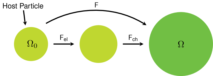
Figure 1: Multiplicative decomposition of the total deformation gradient $\mathsf{F}$ into an elastic part $\mathsf{F}_{\text{el}}$ and a chemical part $\mathsf{F}_{\text{ch}}$, compare [Schoof et al., 2022, Figure 1].

The chemical part of the deformation gradient is defined as $\mathsf{F}_{\text{ch}}(\mkern 1.5mu\overline{\mkern-1.5muc\mkern-1.5mu}\mkern 1.5mu)=\lambda_{\text{ch}}(\mkern 1.5mu\overline{\mkern-1.5muc\mkern-1.5mu}\mkern 1.5mu)\mathsf{Id}$ with $\lambda_{\text{ch}}(\mkern 1.5mu\overline{\mkern-1.5muc\mkern-1.5mu}\mkern 1.5mu)=\sqrt[3]{1+v_{\text{pmv}}c_{\max}\mkern 1.5mu\overline{\mkern-1.5muc\mkern-1.5mu}\mkern 1.5mu}$ and the elastic part $\mathsf{F}_{\text{el}}(\mkern 1.5mu\overline{\mkern-1.5muc\mkern-1.5mu}\mkern 1.5mu,\bm{\nabla}_{0}\vec{u})=\lambda_{\text{ch}}^{\scalebox{0.75}[1.0]{$-$}1}(\mkern 1.5mu\overline{\mkern-1.5muc\mkern-1.5mu}\mkern 1.5mu)\mathsf{F}(\bm{\nabla}_{0}\vec{u})$. All values for the material parameters, such as the partial molar volume $v_{\text{pmv}}$, can be found in Table 5 in Section B.

Free Energy. Guaranteeing a strictly positive entropy production Latz and Zausch [2015, 2011], von Kolzenberg et al. [2022], Schammer et al. [2021] for a thermodynamically consistent model, we base our model approach on a positive free energy $\psi(\mkern 1.5mu\overline{\mkern-1.5muc\mkern-1.5mu}\mkern 1.5mu,\bm{\nabla}_{0}\vec{u})$, considering chemical and mechanical effects:

$$\psi(\mkern 1.5mu\overline{\mkern-1.5muc\mkern-1.5mu}\mkern 1.5mu,\bm{\nabla}_{0}\vec{u})=\psi_{\text{ch}}(\mkern 1.5mu\overline{\mkern-1.5muc\mkern-1.5mu}\mkern 1.5mu)+\psi_{\text{el}}(\mkern 1.5mu\overline{\mkern-1.5muc\mkern-1.5mu}\mkern 1.5mu,\bm{\nabla}_{0}\vec{u}).$$ (2)

The chemical part of the free energy density is formulated using an experimentally obtained OCV curve $U_{\text{OCV}}$ Chan et al. [2007], von Kolzenberg et al. [2022], Keil et al. [2016], Latz and Zausch [2015, 2013]:

$$\rho\psi_{\text{ch}}(\mkern 1.5mu\overline{\mkern-1.5muc\mkern-1.5mu}\mkern 1.5mu)=\scalebox{0.75}[1.0]{$-$}c_{\max}\int_{0}^{\mkern 1.5mu\overline{\mkern-1.5muc\mkern-1.5mu}\mkern 1.5mu}\mathrm{Fa}\,U_{\text{OCV}}(z)\,\mathrm{d}z$$ (3)

with the Faraday constant $\mathrm{Fa}$. We base the model for the elastic part on the linear elastic approach (Saint Venant–Kirchhoff model) as in [Holzapfel, 2010, Section 6.5], [Braess, 2007, Section VI §3] and Castelli et al. [2021], von Kolzenberg et al. [2022]:

$$\rho\psi_{\text{el}}(\mkern 1.5mu\overline{\mkern-1.5muc\mkern-1.5mu}\mkern 1.5mu,\bm{\nabla}_{0}\vec{u})=\frac{1}{2}\mathsf{E}_{\text{el}}\!:\!\bm{\mathds{C}}\left[\mathsf{E}_{\text{el}}\right]\quad\text{and}\quad\bm{\mathds{C}}\left[\mathsf{E}_{\text{el}}\right]=\lambda\operatorname{tr\!}\,(\mathsf{E}_{\text{el}})\mathsf{Id}+2G\mathsf{E}_{\text{el}},$$ (4)

first and second Lamé constants $\lambda=2G\nu/\left(1-2\nu\right)$ and $G=E/\left[2\left(1+2\nu\right)\right]$, Young’s modulus $E$ and Poisson’s ratio $\nu$. The elastic strain tensor $\mathsf{E}_{\text{el}}\in\mathbb{R}_{\text{sym}}^{d,d}$, which is known in literature as the Green–Saint Venant strain tensor or simply the Lagrangian strain tensor [Lubliner, 2006, Section 8.1], is defined as:

$$\mathsf{E}_{\text{el}}(\mkern 1.5mu\overline{\mkern-1.5muc\mkern-1.5mu}\mkern 1.5mu,\bm{\nabla}_{0}\vec{u}) =\frac{1}{2}\left(\mathsf{F}_{\text{el}}^{\textsf{T}}\mathsf{F}_{\text{el}}-\mathsf{Id}\right)=\frac{1}{2}\left(\lambda_{\text{ch}}^{\scalebox{0.75}[1.0]{$-$}2}\mathsf{F}^{\textsf{T}}\mathsf{F}-\mathsf{Id}\right)=\frac{1}{2}\left(\lambda_{\text{ch}}^{\scalebox{0.75}[1.0]{$-$}2}\mathsf{C}-\mathsf{Id}\right).$$ (5)

Chemistry. The change in lithium concentration inside the host material in the Lagrangian domain $\Omega_{0}$ can be described by a continuity equation von Kolzenberg et al. [2022], Schoof et al. [2022, 2023a]:

$$\partial_{t}\mkern 1.5mu\overline{\mkern-1.5muc\mkern-1.5mu}\mkern 1.5mu=\scalebox{0.75}[1.0]{$-$}\bm{\nabla}_{0}\!\cdot\!\vec{N}(\mkern 1.5mu\overline{\mkern-1.5muc\mkern-1.5mu}\mkern 1.5mu,\bm{\nabla}_{0}\vec{u})\qquad\text{in }(0,t_{\text{end}})\times\Omega_{0}.$$ (6)

The lithium flux $\vec{N}$ is given as $\vec{N}(\mkern 1.5mu\overline{\mkern-1.5muc\mkern-1.5mu}\mkern 1.5mu,\bm{\nabla}_{0}\vec{u})=\scalebox{0.75}[1.0]{$-$}m(\mkern 1.5mu\overline{\mkern-1.5muc\mkern-1.5mu}\mkern 1.5mu,\bm{\nabla}_{0}\vec{u})\bm{\nabla}_{0}\mu(\mkern 1.5mu\overline{\mkern-1.5muc\mkern-1.5mu}\mkern 1.5mu,\bm{\nabla}_{0}\vec{u})\in\mathbb{R}^{d}$ with the mobility $m(\mkern 1.5mu\overline{\mkern-1.5muc\mkern-1.5mu}\mkern 1.5mu,\bm{\nabla}_{0}\vec{u})\coloneqq D(\partial_{c}\mu(\mkern 1.5mu\overline{\mkern-1.5muc\mkern-1.5mu}\mkern 1.5mu,\bm{\nabla}_{0}\vec{u}))^{\scalebox{0.75}[1.0]{$-$}1}>0$, the constant diffusion $D>0$ and the chemical potential $\mu(\mkern 1.5mu\overline{\mkern-1.5muc\mkern-1.5mu}\mkern 1.5mu,\bm{\nabla}_{0}\vec{u})\in\mathbb{R}$, derived as the derivative of the free energy density with respect to $c$ von Kolzenberg et al. [2022] as

$$\mu(\mkern 1.5mu\overline{\mkern-1.5muc\mkern-1.5mu}\mkern 1.5mu,\bm{\nabla}_{0}\vec{u})=\partial_{c}(\rho\psi)(\mkern 1.5mu\overline{\mkern-1.5muc\mkern-1.5mu}\mkern 1.5mu,\bm{\nabla}_{0}\vec{u}) =\scalebox{0.75}[1.0]{$-$}\mathrm{Fa}\,U_{\text{OCV}}(\mkern 1.5mu\overline{\mkern-1.5muc\mkern-1.5mu}\mkern 1.5mu)+\partial_{c}\mathsf{E}_{\text{el}}(\mkern 1.5mu\overline{\mkern-1.5muc\mkern-1.5mu}\mkern 1.5mu,\bm{\nabla}_{0}\vec{u})\!:\!\bm{\mathds{C}}[\mathsf{E}_{\text{el}}(\mkern 1.5mu\overline{\mkern-1.5muc\mkern-1.5mu}\mkern 1.5mu,\bm{\nabla}_{0}\vec{u})],$$ (7)

where the last term is additionally given as

$$\partial_{c}\mathsf{E}_{\text{el}}\!:\!\bm{\mathds{C}}[\mathsf{E}_{\text{el}}] =\frac{1}{2}(\scalebox{0.75}[1.0]{$-$}2)\lambda_{\text{ch}}^{\scalebox{0.75}[1.0]{$-$}3}\partial_{c}\lambda_{\text{ch}}\mathsf{C}\!:\!\bm{\mathds{C}}[\mathsf{E}_{\text{el}}]=\scalebox{0.75}[1.0]{$-$}\lambda_{\text{ch}}^{\scalebox{0.75}[1.0]{$-$}3}\frac{v_{\text{pmv}}}{3}\lambda_{\text{ch}}^{\scalebox{0.75}[1.0]{$-$}2}\mathsf{C}\!:\!\bm{\mathds{C}}[\mathsf{E}_{\text{el}}]$$ (8)

$$=\scalebox{0.75}[1.0]{$-$}\frac{v_{\text{pmv}}}{3}\lambda_{\text{ch}}^{\scalebox{0.75}[1.0]{$-$}5}\mathsf{F}^{\textsf{T}}\mathsf{F}\!:\!\bm{\mathds{C}}[\mathsf{E}_{\text{el}}]=-\frac{v_{\text{pmv}}}{3\lambda_{\text{ch}}^{3}}(\lambda_{\text{ch}}^{-2}\mathsf{F}\bm{\mathds{C}}[\mathsf{E}_{\text{el}}])\!:\!\mathsf{F}$$ (9)

due to symmetry of $\bm{\mathds{C}}[\mathsf{E}_{\text{el}}]$ and calculation rules for $\square\!:\!\square=\operatorname{tr\!}\,(\square^{\textsf{T}}\square)$. The representative host particle is cycled with a uniform and constant external flux $N_{\text{ext}}$ with either positive or negative sign. This external flux is applied at the boundary of $\Omega_{0}$ and measured in terms of the charging-rate ($\mathrm{C}$-rate), for which we refer to Castelli et al. [2021] and Deng [2015]. With this definition, the simulation time $t$ and the state of charge (SOC) regarding the maximal capacity Piller et al. [2001] can be related by

$$\mathrm{SOC}=\frac{c_{0}}{c_{\text{max}}}+N_{\text{ext}}\left[$\mathrm{C}$\right]\cdot t[$\mathrm{h}$].$$ (10)

Mechanics. The deformation of the active material is characterized by a static balance of linear momentum von Kolzenberg et al. [2022], Schoof et al. [2022, 2023a], which yields the equation:

$$\vec{0}=\scalebox{0.75}[1.0]{$-$}\bm{\nabla}_{0}\!\cdot\!\mathsf{P}(\mkern 1.5mu\overline{\mkern-1.5muc\mkern-1.5mu}\mkern 1.5mu,\bm{\nabla}_{0}\vec{u})\qquad\text{in }(0,t_{\text{end}})\times\Omega_{0}$$ (11)

with the first Piola–Kirchhoff stress tensor thermodynamical consistent derived as $\mathsf{P}=\partial_{\mathsf{F}}(\rho\psi)=2\mathsf{F}\partial_{\mathsf{C}}(\rho\psi)=\lambda_{\text{ch}}^{\scalebox{0.75}[1.0]{$-$}2}\mathsf{F}\bm{\mathds{C}}\left[\mathsf{E}_{\text{el}}\right]\in\mathbb{R}^{d,d}$ and the Cauchy stress $\bm{\sigma}\textasciiacute\in\mathbb{R}_{\text{sym}}^{d,d}$ in the Eulerian configuration$~{}\Omega$ coupled via $\bm{\sigma}=\mathsf{P}\mathsf{F}^{\textsf{T}}/\det\left(\mathsf{F}\right)$, compare [Holzapfel, 2010, Sections 3.1 and 6.1].

Derivation of the strong formulation. For the implementation of the residual based error estimator, both the divergence of the lithium flux $\vec{N}$ and the divergence of the first Piola–Kirchhoff tensor $\mathsf{P}$ are needed in explicit form. These can be obtained via calculation rules from [Holzapfel, 2010, Section 1.8] for the derivatives. In a first step, $\bm{\nabla}_{0}\!\cdot\!\vec{N}(\mkern 1.5mu\overline{\mkern-1.5muc\mkern-1.5mu}\mkern 1.5mu,\bm{\nabla}_{0}\vec{u})$ is derived. The derivation of the explicit form of $\bm{\nabla}_{0}\!\cdot\!\mathsf{P}(\mkern 1.5mu\overline{\mkern-1.5muc\mkern-1.5mu}\mkern 1.5mu,\bm{\nabla}_{0}\vec{u})$ follows subsequently.

Computation of $\bm{\nabla}_{0}\!\cdot\!\vec{N}$. With the definition of the lithium flux $\vec{N}(\mkern 1.5mu\overline{\mkern-1.5muc\mkern-1.5mu}\mkern 1.5mu,\bm{\nabla}_{0}\vec{u})$, it follows

$$\bm{\nabla}_{0}\!\cdot\!\vec{N} =\bm{\nabla}_{0}\!\cdot\!(\scalebox{0.75}[1.0]{$-$}m(\mkern 1.5mu\overline{\mkern-1.5muc\mkern-1.5mu}\mkern 1.5mu,\bm{\nabla}_{0}\vec{u})\bm{\nabla}_{0}\mu(\mkern 1.5mu\overline{\mkern-1.5muc\mkern-1.5mu}\mkern 1.5mu,\bm{\nabla}_{0}\vec{u}))$$ (12)

$$=\scalebox{0.75}[1.0]{$-$}\bm{\nabla}_{0}m(\mkern 1.5mu\overline{\mkern-1.5muc\mkern-1.5mu}\mkern 1.5mu,\bm{\nabla}_{0}\vec{u})\cdot\bm{\nabla}_{0}\mu(\mkern 1.5mu\overline{\mkern-1.5muc\mkern-1.5mu}\mkern 1.5mu,\bm{\nabla}_{0}\vec{u})-m(\mkern 1.5mu\overline{\mkern-1.5muc\mkern-1.5mu}\mkern 1.5mu,\bm{\nabla}_{0}\vec{u})\bm{\nabla}_{0}\!\cdot\!\bm{\nabla}_{0}\mu(\mkern 1.5mu\overline{\mkern-1.5muc\mkern-1.5mu}\mkern 1.5mu,\bm{\nabla}_{0}\vec{u}))$$ (13)

$$=\scalebox{0.75}[1.0]{$-$}\bm{\nabla}_{0}m(\mkern 1.5mu\overline{\mkern-1.5muc\mkern-1.5mu}\mkern 1.5mu,\bm{\nabla}_{0}\vec{u})\cdot\bm{\nabla}_{0}\mu(\mkern 1.5mu\overline{\mkern-1.5muc\mkern-1.5mu}\mkern 1.5mu,\bm{\nabla}_{0}\vec{u})-m(\mkern 1.5mu\overline{\mkern-1.5muc\mkern-1.5mu}\mkern 1.5mu,\bm{\nabla}_{0}\vec{u})\Delta_{0}\mu(\mkern 1.5mu\overline{\mkern-1.5muc\mkern-1.5mu}\mkern 1.5mu,\bm{\nabla}_{0}\vec{u})).$$ (14)

Furthermore, an application of the chain rule to the mobility yields

$$\bm{\nabla}_{0}m(\mkern 1.5mu\overline{\mkern-1.5muc\mkern-1.5mu}\mkern 1.5mu,\bm{\nabla}_{0}\vec{u})=\partial_{c}m(\mkern 1.5mu\overline{\mkern-1.5muc\mkern-1.5mu}\mkern 1.5mu,\bm{\nabla}_{0}\vec{u})\bm{\nabla}_{0}c+\bm{\nabla}_{0}^{2}\vec{u}\big{[}\partial_{\bm{\nabla}_{0}\vec{u}}m(\mkern 1.5mu\overline{\mkern-1.5muc\mkern-1.5mu}\mkern 1.5mu,\bm{\nabla}_{0}\vec{u})\big{]}$$ (15)

with the Hessian $\bm{\nabla}_{0}^{2}\vec{u}(t,\vec{X}_{0})\in\mathbb{R}^{d,d,d}$ of the displacement $\vec{u}$, and an index reduction of the last two indices in $\bm{\nabla}_{0}^{2}\vec{u}\big{[}\partial_{\bm{\nabla}_{0}\vec{u}}m(\mkern 1.5mu\overline{\mkern-1.5muc\mkern-1.5mu}\mkern 1.5mu,\bm{\nabla}_{0}\vec{u})\big{]}\in\mathbb{R}^{d}$. The first term on the right-hand side in Equation 15 can be formulated by using the definition of the mobility $m(\mkern 1.5mu\overline{\mkern-1.5muc\mkern-1.5mu}\mkern 1.5mu,\bm{\nabla}_{0}\vec{u})=D(\partial_{c}\mu(\mkern 1.5mu\overline{\mkern-1.5muc\mkern-1.5mu}\mkern 1.5mu,\bm{\nabla}_{0}\vec{u}))^{\scalebox{0.75}[1.0]{$-$}1}$ and another application of the chain rule as

$$\partial_{c}m(\mkern 1.5mu\overline{\mkern-1.5muc\mkern-1.5mu}\mkern 1.5mu,\bm{\nabla}_{0}\vec{u})=D\partial_{c}(\partial_{c}\mu(\mkern 1.5mu\overline{\mkern-1.5muc\mkern-1.5mu}\mkern 1.5mu,\bm{\nabla}_{0}\vec{u})^{\scalebox{0.75}[1.0]{$-$}1})=\scalebox{0.75}[1.0]{$-$}D(\partial_{c}\mu(\mkern 1.5mu\overline{\mkern-1.5muc\mkern-1.5mu}\mkern 1.5mu,\bm{\nabla}_{0}\vec{u}))^{\scalebox{0.75}[1.0]{$-$}2}\partial_{c}^{2}\mu(\mkern 1.5mu\overline{\mkern-1.5muc\mkern-1.5mu}\mkern 1.5mu,\bm{\nabla}_{0}\vec{u}).$$ (16)

Using the definition for the chemical potential $\mu(\mkern 1.5mu\overline{\mkern-1.5muc\mkern-1.5mu}\mkern 1.5mu,\bm{\nabla}_{0}\vec{u})=\mu_{\text{ch}}(\mkern 1.5mu\overline{\mkern-1.5muc\mkern-1.5mu}\mkern 1.5mu)+\mu_{\text{el}}(\mkern 1.5mu\overline{\mkern-1.5muc\mkern-1.5mu}\mkern 1.5mu,\bm{\nabla}_{0}\vec{u})$, compare Equation 7, Equation 3 and Equation 4, we have

$$\partial_{c}\mu(\mkern 1.5mu\overline{\mkern-1.5muc\mkern-1.5mu}\mkern 1.5mu,\bm{\nabla}_{0}\vec{u}) =\partial_{c}\mu_{\text{ch}}(\mkern 1.5mu\overline{\mkern-1.5muc\mkern-1.5mu}\mkern 1.5mu)+\partial_{c}\mu_{\text{el}}(\mkern 1.5mu\overline{\mkern-1.5muc\mkern-1.5mu}\mkern 1.5mu,\bm{\nabla}_{0}\vec{u})=\partial_{c}^{2}(\rho\psi)_{\text{ch}}(\mkern 1.5mu\overline{\mkern-1.5muc\mkern-1.5mu}\mkern 1.5mu)+\partial_{c}^{2}(\rho\psi)_{\text{el}}(\mkern 1.5mu\overline{\mkern-1.5muc\mkern-1.5mu}\mkern 1.5mu,\bm{\nabla}_{0}\vec{u})$$ (17)

$$=\scalebox{0.75}[1.0]{$-$}\frac{1}{c_{\max}}\mathrm{Fa}\,U_{\text{OCV}}^{\prime}+\partial_{c}^{2}\mathsf{E}_{\text{el}}\!:\!\bm{\mathds{C}}[\mathsf{E}_{\text{el}}]+\partial_{c}\mathsf{E}_{\text{el}}\!:\!\bm{\mathds{C}}[\partial_{c}\mathsf{E}_{\text{el}}]$$ (18)

and

$$\partial_{c}^{2}\mu(\mkern 1.5mu\overline{\mkern-1.5muc\mkern-1.5mu}\mkern 1.5mu,\bm{\nabla}_{0}\vec{u}) =\partial_{c}^{2}\mu_{\text{ch}}(\mkern 1.5mu\overline{\mkern-1.5muc\mkern-1.5mu}\mkern 1.5mu)+\partial_{c}^{2}\mu_{\text{el}}(\mkern 1.5mu\overline{\mkern-1.5muc\mkern-1.5mu}\mkern 1.5mu,\bm{\nabla}_{0}\vec{u})=\partial_{c}^{3}(\rho\psi)_{\text{ch}}(\mkern 1.5mu\overline{\mkern-1.5muc\mkern-1.5mu}\mkern 1.5mu)+\partial_{c}^{3}(\rho\psi)_{\text{el}}(\mkern 1.5mu\overline{\mkern-1.5muc\mkern-1.5mu}\mkern 1.5mu,\bm{\nabla}_{0}\vec{u})$$ (19)

$$=\scalebox{0.75}[1.0]{$-$}\frac{1}{c_{\max}^{2}}\mathrm{Fa}\,U_{\text{OCV}}^{\prime\prime}+\partial_{c}^{3}\mathsf{E}_{\text{el}}\!:\!\bm{\mathds{C}}[\mathsf{E}_{\text{el}}]+3\partial_{c}^{2}\mathsf{E}_{\text{el}}\!:\!\bm{\mathds{C}}[\partial_{c}\mathsf{E}_{\text{el}}].$$ (20)

Furthermore, we need

$$\partial_{\bm{\nabla}_{0}\vec{u}}m(\mkern 1.5mu\overline{\mkern-1.5muc\mkern-1.5mu}\mkern 1.5mu,\bm{\nabla}_{0}\vec{u}) =D\partial_{\bm{\nabla}_{0}\vec{u}}(\partial_{c}\mu(\mkern 1.5mu\overline{\mkern-1.5muc\mkern-1.5mu}\mkern 1.5mu,\bm{\nabla}_{0}\vec{u}))^{{\scalebox{0.75}[1.0]{$-$}1}}$$ (21)

$$=\scalebox{0.75}[1.0]{$-$}D(\partial_{c}\mu(\mkern 1.5mu\overline{\mkern-1.5muc\mkern-1.5mu}\mkern 1.5mu,\bm{\nabla}_{0}\vec{u}))^{\scalebox{0.75}[1.0]{$-$}2}\partial_{\bm{\nabla}_{0}\vec{u}}\partial_{c}\mu(\mkern 1.5mu\overline{\mkern-1.5muc\mkern-1.5mu}\mkern 1.5mu,\bm{\nabla}_{0}\vec{u})$$ (22)

with the last term

$$\partial_{\bm{\nabla}_{0}\vec{u}}\partial_{c}\mu(\mkern 1.5mu\overline{\mkern-1.5muc\mkern-1.5mu}\mkern 1.5mu,\bm{\nabla}_{0}\vec{u}) =\partial_{\bm{\nabla}_{0}\vec{u}}\partial_{c}\big{(}\mu_{\text{ch}}(\mkern 1.5mu\overline{\mkern-1.5muc\mkern-1.5mu}\mkern 1.5mu)+\mu_{\text{el}}(\mkern 1.5mu\overline{\mkern-1.5muc\mkern-1.5mu}\mkern 1.5mu,\bm{\nabla}_{0}\vec{u})\big{)}=\partial_{\bm{\nabla}_{0}\vec{u}}\partial_{c}\mu_{\text{el}}(\mkern 1.5mu\overline{\mkern-1.5muc\mkern-1.5mu}\mkern 1.5mu,\bm{\nabla}_{0}\vec{u})$$ (23)

$$=\partial_{\bm{\nabla}_{0}\vec{u}}\big{(}\partial_{c}^{2}\mathsf{E}_{\text{el}}\!:\!\bm{\mathds{C}}[\mathsf{E}_{\text{el}}]+\partial_{c}\mathsf{E}_{\text{el}}\!:\!\bm{\mathds{C}}[\partial_{c}\mathsf{E}_{\text{el}}]\big{)}$$ (24)

$$=\partial_{\bm{\nabla}_{0}\vec{u}}\partial_{c}^{2}\mathsf{E}_{\text{el}}[\bm{\mathds{C}}[\mathsf{E}_{\text{el}}]]+\partial_{\bm{\nabla}_{0}\vec{u}}(\bm{\mathds{C}}[\mathsf{E}_{\text{el}}])[\partial_{c}^{2}\mathsf{E}_{\text{el}}]$$ (25)

$$\quad+2\partial_{\bm{\nabla}_{0}\vec{u}}\partial_{c}\mathsf{E}_{\text{el}}[\bm{\mathds{C}}[\partial_{c}\mathsf{E}_{\text{el}}]].$$ (26)

The second term in Equation 25 can be computed with a symmetric tensor $\mathsf{S}\in\mathbb{R}_{\text{sym}}^{d,d}$ as

$$\partial_{\bm{\nabla}_{0}\vec{u}}(\bm{\mathds{C}}[\mathsf{E}_{\text{el}}])[\mathsf{S}] =2G\partial_{\bm{\nabla}_{0}\vec{u}}\mathsf{E}_{\text{el}}[\mathsf{S}]+\lambda\mathsf{Id}\partial_{\bm{\nabla}_{0}\vec{u}}\mathsf{E}_{\text{el}}[\mathsf{S}]$$ (27)

$$=(2G+\lambda)\partial_{\bm{\nabla}_{0}\vec{u}}\mathsf{E}_{\text{el}}[\mathsf{S}]$$ (28)

$$=(2G+\lambda)\lambda_{\text{ch}}^{\scalebox{0.75}[1.0]{$-$}2}\mathsf{F}\mathsf{S}$$ (29)

and the term in Equation 26 as

$$\partial_{\bm{\nabla}_{0}\vec{u}}(\partial_{c}\mathsf{E}_{\text{el}}\!:\!\bm{\mathds{C}}[\partial_{c}\mathsf{E}_{\text{el}}]) =2\partial_{\bm{\nabla}_{0}\vec{u}}\partial_{c}\mathsf{E}_{\text{el}}[\bm{\mathds{C}}[\partial_{c}\mathsf{E}_{\text{el}}]]$$ (30)

$$=2((\scalebox{0.75}[1.0]{$-$}2)\frac{v_{\text{pmv}}}{3}\lambda_{\text{ch}}^{\scalebox{0.75}[1.0]{$-$}5}\mathsf{F})\,(2G\partial_{c}\mathsf{E}_{\text{el}}+\lambda\operatorname{tr\!}\,(\partial_{c}\mathsf{E}_{\text{el}})\mathsf{Id}).$$ (31)

Following Equation 12 – Equation 14, we have in total

$$\bm{\nabla}_{0}\!\cdot\!\vec{N}(\mkern 1.5mu\overline{\mkern-1.5muc\mkern-1.5mu}\mkern 1.5mu,\bm{\nabla}_{0}\vec{u}) =\scalebox{0.75}[1.0]{$-$}\big{(}\partial_{c}m(\mkern 1.5mu\overline{\mkern-1.5muc\mkern-1.5mu}\mkern 1.5mu,\bm{\nabla}_{0}\vec{u})\bm{\nabla}_{0}c+\bm{\nabla}_{0}^{2}\vec{u}[\partial_{\bm{\nabla}_{0}\vec{u}}m(\mkern 1.5mu\overline{\mkern-1.5muc\mkern-1.5mu}\mkern 1.5mu,\bm{\nabla}_{0}\vec{u})]\big{)}\cdot\bm{\nabla}_{0}\mu(\mkern 1.5mu\overline{\mkern-1.5muc\mkern-1.5mu}\mkern 1.5mu,\bm{\nabla}_{0}\vec{u})$$ (32)

$$\quad-m(\mkern 1.5mu\overline{\mkern-1.5muc\mkern-1.5mu}\mkern 1.5mu,\bm{\nabla}_{0}\vec{u})\Delta_{0}\mu(\mkern 1.5mu\overline{\mkern-1.5muc\mkern-1.5mu}\mkern 1.5mu,\bm{\nabla}_{0}\vec{u})).$$ (33)

Computation of $\bm{\nabla}_{0}\!\cdot\!\mathsf{P}$. The divergence of the first Piola–Kirchhoff tensor $\mathsf{P}(\mkern 1.5mu\overline{\mkern-1.5muc\mkern-1.5mu}\mkern 1.5mu,\bm{\nabla}_{0}\vec{u})$ is given as

$$\bm{\nabla}_{0}\!\cdot\!\mathsf{P}(\mkern 1.5mu\overline{\mkern-1.5muc\mkern-1.5mu}\mkern 1.5mu,\bm{\nabla}_{0}\vec{u}) =\bm{\nabla}_{0}\!\cdot\!\big{(}\lambda_{\text{ch}}^{\scalebox{0.75}[1.0]{$-$}2}(\mkern 1.5mu\overline{\mkern-1.5muc\mkern-1.5mu}\mkern 1.5mu)\mathsf{F}(\bm{\nabla}_{0}\vec{u})\bm{\mathds{C}}[\mathsf{E}_{\text{el}}(\mkern 1.5mu\overline{\mkern-1.5muc\mkern-1.5mu}\mkern 1.5mu,\bm{\nabla}_{0}\vec{u})]\big{)}$$ (34)

$$=\mathsf{F}\bm{\mathds{C}}[\mathsf{E}_{\text{el}}]\bm{\nabla}_{0}\lambda_{\text{ch}}^{\scalebox{0.75}[1.0]{$-$}2}+\lambda_{\text{ch}}^{\scalebox{0.75}[1.0]{$-$}2}\bm{\nabla}_{0}\!\cdot\!(\mathsf{F}\bm{\mathds{C}}[\mathsf{E}_{\text{el}}])$$ (35)

$$=(\scalebox{0.75}[1.0]{$-$}2)\frac{v_{\text{pmv}}}{3}\lambda_{\text{ch}}^{\scalebox{0.75}[1.0]{$-$}5}\mathsf{F}\bm{\mathds{C}}[\mathsf{E}_{\text{el}}]\bm{\nabla}_{0}c+\lambda_{\text{ch}}^{\scalebox{0.75}[1.0]{$-$}2}\bm{\nabla}_{0}\!\cdot\!(\mathsf{F}\bm{\mathds{C}}[\mathsf{E}_{\text{el}}])$$ (36)

$$=\partial_{\bm{\nabla}_{0}\vec{u}}\partial_{c}\mathsf{E}_{\text{el}}[\bm{\mathds{C}}[\mathsf{E}_{\text{el}}]]\bm{\nabla}_{0}c+\lambda_{\text{ch}}^{\scalebox{0.75}[1.0]{$-$}2}\bm{\nabla}_{0}\!\cdot\!(\mathsf{F}\bm{\mathds{C}}[\mathsf{E}_{\text{el}}]).$$ (37)

The final term computes to

$$\bm{\nabla}_{0}\!\cdot\!\big{(}\mathsf{F}(\bm{\nabla}_{0}\vec{u})\bm{\mathds{C}}[\mathsf{E}_{\text{el}}(c,\bm{\nabla}_{0}\vec{u})]\big{)} =\bm{\nabla}_{0}\mathsf{F}(\bm{\nabla}_{0}\vec{u})[\bm{\mathds{C}}[\mathsf{E}_{\text{el}}(c,\bm{\nabla}_{0}\vec{u})]]$$ (38)

$$\quad+\mathsf{F}(\bm{\nabla}_{0}\vec{u})\bm{\nabla}_{0}\!\cdot\!(\bm{\mathds{C}}[\mathsf{E}_{\text{el}}(c,\bm{\nabla}_{0}\vec{u})])$$ (39)

with $\bm{\nabla}_{0}\mathsf{F}(\bm{\nabla}_{0}\vec{u})[\mathsf{S}]=\bm{\nabla}_{0}^{2}\vec{u}[\mathsf{S}]$ with a symmetric tensor $\mathsf{S}\in\mathbb{R}_{\text{sym}}^{d,d}$. The last term is turned into an explicit form using $\bm{\nabla}_{0}\!\cdot\!\mathsf{A}=\operatorname{tr\!}\,(\bm{\nabla}_{0}\mathsf{A})=\bm{\nabla}_{0}\mathsf{A}[\mathsf{Id}]$:

$$\bm{\nabla}_{0}\!\cdot\!(\bm{\mathds{C}}[\mathsf{E}_{\text{el}}]) =2G\bm{\nabla}_{0}\!\cdot\!\mathsf{E}_{\text{el}}(\mkern 1.5mu\overline{\mkern-1.5muc\mkern-1.5mu}\mkern 1.5mu,\bm{\nabla}_{0}\vec{u})+\lambda\bm{\nabla}_{0}\!\cdot\!\big{(}\operatorname{tr\!}\,(\mathsf{E}_{\text{el}}(\mkern 1.5mu\overline{\mkern-1.5muc\mkern-1.5mu}\mkern 1.5mu,\bm{\nabla}_{0}\vec{u}))\mathsf{Id}\big{)}$$ (40)

$$=2G\bm{\nabla}_{0}\!\cdot\!\Big{(}\frac{1}{2}(\lambda_{\text{ch}}^{\scalebox{0.75}[1.0]{$-$}2}(\mkern 1.5mu\overline{\mkern-1.5muc\mkern-1.5mu}\mkern 1.5mu)\mathsf{C}(\bm{\nabla}_{0}\vec{u})-\mathsf{Id})\Big{)}$$ (41)

$$\quad+\lambda\bm{\nabla}_{0}\!\cdot\!\Big{(}\operatorname{tr\!}\,(\frac{1}{2}(\lambda_{\text{ch}}^{\scalebox{0.75}[1.0]{$-$}2}(\mkern 1.5mu\overline{\mkern-1.5muc\mkern-1.5mu}\mkern 1.5mu)\mathsf{C}(\bm{\nabla}_{0}\vec{u})-\mathsf{Id}))\mathsf{Id}\Big{)}$$ (42)

$$=2G\frac{1}{2}\big{(}\mathsf{C}\bm{\nabla}_{0}\lambda_{\text{ch}}^{\scalebox{0.75}[1.0]{$-$}2}+\lambda_{\text{ch}}^{\scalebox{0.75}[1.0]{$-$}2}\bm{\nabla}_{0}\!\cdot\!\mathsf{C}\big{)}+\lambda\frac{1}{2}\bm{\nabla}_{0}\!\cdot\!\big{(}\lambda_{\text{ch}}^{\scalebox{0.75}[1.0]{$-$}2}\operatorname{tr\!}\,(\mathsf{C})\mathsf{Id}\big{)}$$ (43)

$$=G\big{(}\mathsf{C}(\scalebox{0.75}[1.0]{$-$}2)\lambda_{\text{ch}}^{\scalebox{0.75}[1.0]{$-$}3}\partial_{c}\lambda_{\text{ch}}\bm{\nabla}_{0}c+\lambda_{\text{ch}}^{\scalebox{0.75}[1.0]{$-$}2}\bm{\nabla}_{0}\mathsf{C}[\mathsf{Id}]\big{)}$$ (44)

$$\quad+\lambda\frac{1}{2}\mathsf{Id}\bm{\nabla}_{0}\big{(}\lambda_{\text{ch}}^{\scalebox{0.75}[1.0]{$-$}2}\operatorname{tr\!}\,(\mathsf{C})\big{)}+\vec{0}$$ (45)

$$=G\big{(}\mathsf{C}(\scalebox{0.75}[1.0]{$-$}2)\lambda_{\text{ch}}^{\scalebox{0.75}[1.0]{$-$}3}\frac{v_{\text{pmv}}}{3}\lambda_{\text{ch}}^{\scalebox{0.75}[1.0]{$-$}2}\bm{\nabla}_{0}c+\lambda_{\text{ch}}^{\scalebox{0.75}[1.0]{$-$}2}\bm{\nabla}_{0}^{2}\vec{u}[\partial_{\bm{\nabla}\vec{u}}\mathsf{F}[\partial_{\mathsf{F}}\mathsf{C}[\mathsf{Id}]]]\big{)}$$ (46)

$$\quad+\lambda\frac{1}{2}\big{(}\operatorname{tr\!}\,(\mathsf{C})\bm{\nabla}_{0}\lambda_{\text{ch}}^{\scalebox{0.75}[1.0]{$-$}2}+\lambda_{\text{ch}}^{\scalebox{0.75}[1.0]{$-$}2}\bm{\nabla}_{0}\operatorname{tr\!}\,(\mathsf{C})\big{)}$$ (47)

$$=G\big{(}2\partial_{c}\mathsf{E}_{\text{el}}\bm{\nabla}_{0}c+\lambda_{\text{ch}}^{\scalebox{0.75}[1.0]{$-$}2}\bm{\nabla}_{0}^{2}\vec{u}[2\mathsf{F}]\big{)}$$ (48)

$$\quad+\frac{1}{2}\lambda\big{(}\operatorname{tr\!}\,(\mathsf{C})(\scalebox{0.75}[1.0]{$-$}2)\lambda_{\text{ch}}^{\scalebox{0.75}[1.0]{$-$}3}\frac{v_{\text{pmv}}}{3}\lambda_{\text{ch}}^{\scalebox{0.75}[1.0]{$-$}2}\bm{\nabla}_{0}c+\lambda_{\text{ch}}^{\scalebox{0.75}[1.0]{$-$}2}\bm{\nabla}_{0}^{2}\vec{u}[\partial_{\bm{\nabla}\vec{u}}\mathsf{F}[\partial_{\mathsf{F}}\mathsf{C}[\mathsf{Id}]]]\big{)}$$ (49)

$$=2G\big{(}\partial_{c}\mathsf{E}_{\text{el}}\bm{\nabla}_{0}c+\lambda_{\text{ch}}^{\scalebox{0.75}[1.0]{$-$}2}\bm{\nabla}_{0}^{2}\vec{u}[\mathsf{F}]\big{)}+\lambda\big{(}\operatorname{tr\!}\,(\partial_{c}\mathsf{E}_{\text{el}})\bm{\nabla}_{0}c+\lambda_{\text{ch}}^{\scalebox{0.75}[1.0]{$-$}2}\bm{\nabla}_{0}^{2}\vec{u}[\mathsf{F}]\big{)}$$ (50)

$$=\bm{\mathds{C}}[\partial_{c}\mathsf{E}_{\text{el}}]\bm{\nabla}_{0}c+(2G+\lambda)\lambda_{\text{ch}}^{\scalebox{0.75}[1.0]{$-$}2}\bm{\nabla}_{0}^{2}\vec{u}[\mathsf{F}].$$ (51)

Now, we have all terms to apply the residual based error estimator.

3 Numerical Solution Procedure

Now, all important aspects for the numerical treatment and the three adaptive refinement possibilities, being numerically compared, are shortly introduced.

Problem Formulation. Firstly, we refer to Table 4 for the normalization of our used model parameters. From now on, we consider only the dimensionless variables without any accentuation. Secondly, we obtain our problem formulation of the dimensionless initial boundary value problem from Section 2: let $t_{\text{end}}>0$ the final simulation time and $\Omega_{0}$ a bounded electrode particle as reference configuration with dimension $d=3$. Find the normalized concentration $c\colon[0,t_{\text{end}}]\times\overline{\Omega}_{0}\rightarrow[0,1]$, the chemical potential $\mu\colon[0,t_{\text{end}}]\times\overline{\Omega}_{0}\rightarrow\mathbb{R}$ and the displacement $\vec{u}\colon[0,t_{\text{end}}]\times\overline{\Omega}_{0}\rightarrow\mathbb{R}^{d}$ satisfying

$$\partial_{t}c =\scalebox{0.75}[1.0]{$-$}\bm{\nabla}_{0}\!\cdot\!\vec{N}(c,\bm{\nabla}_{0}\vec{u}) \text{in }(0,t_{\text{end}})\times\Omega_{0},$$ (52a)

$$\mu(c,\bm{\nabla}_{0}\vec{u}) =\partial_{c}(\rho\psi)(c,\bm{\nabla}_{0}\vec{u}) \text{in }(0,t_{\text{end}})\times\Omega_{0},$$ (52b)

$$\vec{0} =\scalebox{0.75}[1.0]{$-$}\bm{\nabla}_{0}\!\cdot\!\mathsf{P}(c,\bm{\nabla}_{0}\vec{u}) \text{in }(0,t_{\text{end}})\times\Omega_{0},$$ (52c)

$$\vec{N}(c,\bm{\nabla}_{0}\vec{u})\cdot\vec{n}_{0} =N_{\text{ext}} \text{on }(0,t_{\text{end}})\times\partial\Omega_{0},$$ (52d)

$$\mathsf{P}(c,\bm{\nabla}_{0}\vec{u})\cdot\vec{n}_{0} =\vec{0} \text{on }(0,t_{\text{end}})\times\partial\Omega_{0},$$ (52e)

$$c(0,\bm{\cdot}) =c_{0} \text{in }\Omega_{0}$$ (52f)

with an initial condition $c_{0}$ being consistent with the boundary conditions. Our quantities of interest are the concentration $c$ and the Cauchy stress $\sigma$, computed in a postprocessing stress with the help of the three solution variables. In the case of lithiation of the host particle, the sign of the external lithium flux $N_{\text{ext}}$ is positive. Contrarily, in the case of delithiation, the sign of the external lithium flux is negative. Appropriate boundary conditions for the displacement are used to exclude rigid body motions. The original formulation of the chemical deformation gradient $\mathsf{F}_{\text{ch}}$ is written for the three-dimensional case, however, it is applicable and mathematically valid also for all variables and equations in lower dimensions as well.

Numerical Solution Procedure. We apply the finite element method on the model equations in Equation 52 for the spatial discretization similar to Schoof et al. [2023a] and Castelli et al. [2021]. Furthermore, we use the family of numerical differentiation formulas (NDFs) in a variable-step, variable-order algorithm Reichelt et al. [1997], Shampine and Reichelt [1997], Shampine et al. [1999, 2003], because the properties of the resulting differential algebraic equation $(\text{DAE})$ are similar to stiff ordinary differential equations Castelli et al. [2021]. The change in time step sizes $\tau_{n}$ and order $k_{n}$ is handled by an error control, see Algorithm 1 in Castelli et al. [2021]. The adaptivity of Algorithm 1 is then achieved with a mixed error control using thresholds $\operatorname{RelTol}_{t}$, $\operatorname{AbsTol}_{t}$, $\operatorname{RelTol}_{x}$ and $\operatorname{AbsTol}_{x}$, compare Castelli et al. [2021] and [Shampine et al., 2003, Section 1.4]. Finally, the resulting nonlinear system is linearized with the Newton–Raphson method and is solved for the updates with a direct LU-decomposition. In this work, we compare three error estimators for the local criterion of the adaptive mesh refinement and coarsening: the Kelly-, the gradient recovery- and the residual based error estimator, as described in the introduction. For later use, we state the definition of the residual:

$$\vec{R}_{h}^{n+1}=\begin{pmatrix}\frac{1}{\hat{\tau}_{n}}\mathsf{M}(\vec{y}^{n+1}-\vec{\Phi}^{n})+\bm{\nabla}_{0}\!\cdot\!\vec{N}_{h}^{n+1}\\ \mu_{h}^{n+1}-\partial_{c}(\rho\psi)_{h}^{n+1}\\ \bm{\nabla}_{0}\!\cdot\!\mathsf{P}_{h}^{n+1}\end{pmatrix}$$ (53)

with the mass matrix $\mathsf{M}$ of the finite element space of dimension $N$ regarding the concentration $c$, the discrete solution vector $\vec{y}\colon[0,t_{\text{end}}]\rightarrow\mathbb{R}^{(2+d)N}$ with $\vec{y}^{n+1}\approx\vec{y}(t_{n+1})$, containing all three discrete components $c_{h}$, $\mu_{h}$ and $\vec{u}_{h}$. $\hat{\tau}_{n}$ is a modified time step size with coefficients of the selected order $k_{n}$ at time $t_{n}$.

In total, the residual based error estimation $\text{est}_{x}$ can be split up into a cell fraction and a face fraction, whereby the latter one includes also the boundary parts. For the first one, we sum up the $L^{2}$-norm of the residual over all cells $K$ of our triangulation, weighted with the largest diagonal of the cell $h_{K}$ in Equation 54. For the latter one, we add up all jumps $[\![\bm{\cdot}]\!]$ of the function in square brackets at the inner faces $\mathcal{F}^{\mathrm{o}}$ of all cells in Equation 56 and additionally as well as the boundary conditions for all faces $\mathcal{F}^{\partial\Omega_{\text{0}}}$ at all boundary cells in Equation 57. Both face parts are weighted with $h_{K}/24$ as proposed in [Ainsworth and Oden, 2000, Section 4.2]. In summary, we have the overall error estimator with constants $\gamma_{1}>0$ and $\gamma_{2}>0$ computed as:

$$\text{est}_{x}^{2} \coloneqq\gamma_{1}\eta_{\text{cell}}^{2}+\gamma_{2}\eta_{\text{face}}^{2}$$ (54)

$$=\gamma_{1}h_{K}^{2}\sum_{K}\|\textbf{R}_{h}^{n+1}\|_{L^{2}(K)}^{2}$$ (55)

$$\quad+\gamma_{2}\frac{h_{K}}{24}\sum_{F\in\mathcal{F}^{\mathrm{o}}\cap K}\Bigl{(}\|[\![\vec{N}_{h}^{n+1}\cdot\vec{n}_{0}]\!]\|_{L^{2}(F)}^{2}+\||[\![\mathsf{P}_{h}^{n+1}\cdot\vec{n}_{0}]\!]|_{2}^{2}\|_{L^{2}(F)}^{2}\Bigr{)}$$ (56)

$$\quad+\gamma_{2}\frac{h_{K}}{24}\sum_{F\in\mathcal{F}^{\partial\Omega_{\text{0}}}\cap K}\Bigl{(}\|\vec{N}_{h}^{n+1}\cdot\vec{n}_{0}-N_{\text{ext}}\|_{L^{2}(F)}^{2}+\||\mathsf{P}_{h}^{n+1}\cdot\vec{n}_{0}-\vec{0}|_{2}^{2}\|_{L^{2}(F)}^{2}\Bigr{)}.$$ (57)

Keep in mind that we have to add further boundary conditions for some additional artificial boundaries for the specified computational domain as explained in Subsection 4.1.

4 Numerical Studies

In this section, we specify our simulation setup, present and discuss our simulation results of the comparison of the three spatial refinement strategies for the presented model of Section 2.

4.1 Simulation Setup

We choose aSi as host material for our derived theory with material parameters and dimensionless values given in Table 5. The used experimental OCV-curve is taken from [von Kolzenberg et al., 2022, Equation (SI-51)] and displayed in [Schoof et al., 2022, Figure 2]. For lithiation, we apply an external constant lithium flux $N_{\text{ext}}=1$\mathrm{C}$$ and for delithiation, the value $N_{\text{ext}}=\scalebox{0.75}[1.0]{$-$}1$\mathrm{C}$$ is given. Following von Kolzenberg et al. [2022], Schoof et al. [2023a, b], we start with a constant concentration $c_{0}=0.02$ and determine one cycle period of lithiation or delithiation with a duration $0.90\,$\mathrm{h}$$, so we are in the range of $\text{SOC}\in[0.02,0.92]$ and time $t\in[0.0~{}$\mathrm{h}$,0.90\,$\mathrm{h}$]$ for lithiation, followed by a delithiation with the same duration of $0.90~{}$\mathrm{h}$$ and decreasing SOC. After the discharging, another charging cycle is added and so on. For a total simulation time of $t=2.7~{}$\mathrm{h}$$, we have following cycles: charging–discharging–charging.

Geometrical Setup. Similar to Schoof et al. [2023b], we choose a representative 3D spherical particle with domain $\Omega_{0}$, reduced to a 1D computational domain $\Omega_{\text{com}}$ as shown in Figure 2 in terms of the radial variable $r$, and a quarter ellipsoid as computational domain $\Omega_{\text{com}}$ resulting from a 3D nanowire domain $\Omega$ with no changes in $z$-direction and symmetry around the $x$- and $y$-axis as in Figure 3. For the adaption of the quadrature weight and the initial conditions, we refer to the literature cited.

Figure 2: Dimension reduction of a 3D unit sphere to the 1D unit interval with spherical symmetry, based on [Castelli, 2021, Figure B.1].

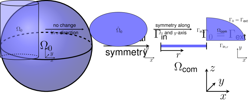
Figure 3: Dimension reduction of a 3D elliptical nanowire to the 2D quarter ellipsoid, based on [Schoof et al., 2023a, Figure 5].

However, we have to mention the additional artificial inner boundary conditions, indicated with the subscript $\square_{\text{in}}$. For the 1D computational domain, we have

$$\vec{N}\cdot\vec{n}_{0}=0,\quad u=0,\quad\text{on }(0,t_{\text{end}}\times\Gamma_{\text{in}})$$ (58)

and for the 2D computational domain

$$\vec{N}\cdot\vec{n}_{0} =0,\quad u_{y} =0,\quad \text{on }(0,t_{\text{end}}\times\Gamma_{\text{in},x}),$$ (59)

$$\vec{N}\cdot\vec{n}_{0} =0,\quad u_{x} =0,\quad \text{on }(0,t_{\text{end}}\times\Gamma_{\text{in},y}).$$ (60)

These new terms also appear in the computation of the boundary face terms of the residual base error estimator of Equation 57. For the 1D computational domain, we have to add

$$\gamma_{2}\frac{h_{K}}{24}\sum_{F\in\mathcal{F}^{\Gamma_{\text{in}}}\cap K}\Bigl{(}\|\vec{N}_{h}^{n+1}\cdot\vec{n}_{0}-0\|_{L^{2}(F)}^{2}+\|u-0\|_{L^{2}(F)}^{2}\Bigr{)}$$ (61)

to the already mentioned face terms and for the 2D computational domain

$$\gamma_{2}\frac{h_{K}}{24}\sum_{F\in\mathcal{F}^{\Gamma_{\text{in},x}}\cap K}\Bigl{(}\|\vec{N}_{h}^{n+1}\cdot\vec{n}_{0}-0\|_{L^{2}(F)}^{2}+\|u_{y}-0\|_{L^{2}(F)}^{2}\Bigr{)}$$ (62)

$$+ \gamma_{2}\frac{h_{K}}{24}\sum_{F\in\mathcal{F}^{\Gamma_{\text{in},y}}\cap K}\Bigl{(}\|\vec{N}_{h}^{n+1}\cdot\vec{n}_{0}-0\|_{L^{2}(F)}^{2}+\|u_{x}-0\|_{L^{2}(F)}^{2}\Bigr{)}.$$ (63)

Implementation Details. We use an isoparametric fourth-order Lagrangian finite element method with isoparametric representation of the curved boundary for our numerical simulations. The C++ finite element library deal.II Arndt et al. [2023] is taken as basis as well as the interface to the Trilinos library[Trilinos Project Team, 2023, Version 12.8.1] and the UMFPACK package [Davis, 2004, Version 5.7.8] for the LU-decomposition. All simulations for the 1D computational domain are performed on a desktop computer with $64\text{\,}\mathrm{GB}$ RAM, Intel i5-9500 CPU, GCC compiler version 10.5 and operating system Ubuntu 20.04.6 LTS, whereas the simulations for the 2D computational domain are executed with GCC compiler version 12.1 with a single node of the BwUniCluster 2.0 with 40 Intel Xeon Gold 6230 with $2.1\text{\,}\mathrm{GHz}$ and $96\text{\,}\mathrm{GB}$ RAM, on bw HPC Team [2024]. The highly resolved solution, which is used to compute the error in Table 1, is also computed on BwUniCluster 2.0. Unless otherwise stated, we set for the space and time adaptive algorithm following parameters: tolerances $\operatorname{RelTol}_{t}=\operatorname{RelTol}_{x}=$1\text{\times}{10}^{-5}$$, $\operatorname{AbsTol}_{t}=\operatorname{AbsTol}_{x}=$1\text{\times}{10}^{-8}$$, initial time step size $\tau_{0}=$1\text{\times}{10}^{-6}$$, final simulation time $t_{\text{end}}=2.7$, maximal time step size $\tau_{\max}=0.1$, number of initial refinements 7, minimal refinement level 3 for the 1D computational domain and level 1 for the 2D computational domain, maximal refinement level of 20 and marking parameters for the local mesh coarsening and refinement, $\theta_{\mathrm{c}}=0.05$ and $\theta_{\mathrm{r}}=0.3$. Furthermore, we use automatic differentiation (AD) for the computation of the Newton matrix Schoof et al. [2023b] and OpenMP Version 4.5 for shared memory parallelization for assembling the residuals.

4.2 Numerical Results

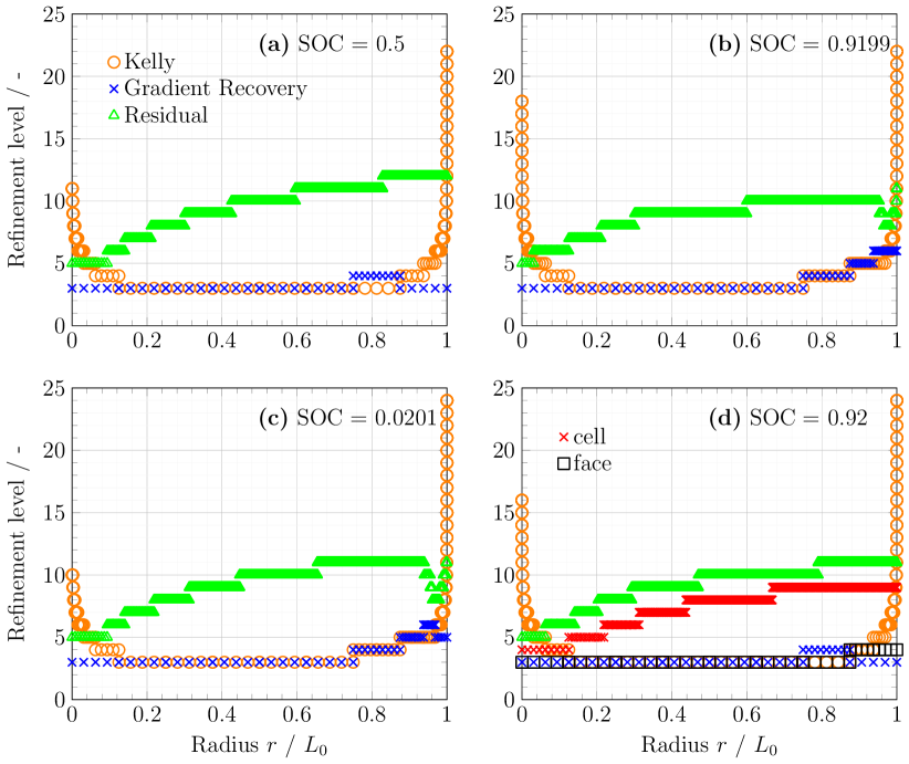
Figure 4: Comparison of three different refinement strategies (Kelly error estimator, gradient recovery error estimator and residual based error estimator with $\gamma_{1}=1.0$ and $\gamma_{2}=1.0$) over the particle radius at different SOC: $\text{SOC}=0.5$ in (a), $\text{SOC}=0.9199$ in (b), $\text{SOC}=0.0201$ in (c) and $\text{SOC}=0.92$ in (d), whereas the last one contains also the two fractions of the cell and the face error of the residual based error estimator.

Example 1: 1D Spherical Symmetry. In a first step, we compare the three adaptive refinement strategies at four different time steps during our simulation with $t_{\text{end}}=2.7~{}$\mathrm{h}$$. Figure 4 shows the refinement levels for the Kelly error estimator, the gradient recovery estimator and the residual based error estimator with $\gamma_{1}=1.0$ and $\gamma_{2}=1.0$ over the particle radius at $t=0.48~{}$\mathrm{h}$$ corresponding to $\text{SOC}=0.50$ in Subfigure (a), at $t=0.9001~{}$\mathrm{h}$$ corresponding to $\text{SOC}=0.9199$ in Subfigure (b), at $t=1.8001~{}$\mathrm{h}$$ corresponding to $\text{SOC}=0.0201$ in Subfigure (c) and the final simulation time at $t_{\text{end}}=2.7~{}$\mathrm{h}$$ corresponding to $\text{SOC}=0.92$ in Subfigure (d). For the simulation with the Kelly error estimator, we have increased the maximal refinement level to 25 and also updated the tolerances to $\operatorname{RelTol}_{t}=\operatorname{RelTol}_{x}=$1\text{\times}{10}^{-4}$$, $\operatorname{AbsTol}_{t}=\operatorname{AbsTol}_{x}=$1\text{\times}{10}^{-7}$$ to get a stable simulation. Is is clearly evident that the Kelly error estimator over-refines the boundary parts, since the estimator has no information about the exact boundary terms. The gradient recovery estimator has only at some range around $r=0.8$ a higher refinement level in Figure 4(a) and Figure 4(d), whereas shortly after the sign change of the external lithium flux also a higher refinement level is reached at the particle surface around $r=1.0$ in the other two subfigures. The residual based error estimator features some stair-like behavior with increasing refinement level from smaller to larger radius values in Figure 4(a) and Figure 4(d). Shortly after the change of the sign of the lithium flux in Figure 4(b) and Figure 4(c), there is a drop of the refinement level at the particle surface. This could be explained by the large influence of the cell error fraction on the residual based refinement strategy, compare the two cell and face fractions, which are additionally added in Figure 4(d). Due to the change of the lithium flux, the cell fraction error is smaller (since the lithium flux direction close to particle surface around $r=1.0$ has also changed) and therefore, a smaller refinement level is sufficient. The behavior of the face error of the residual based strategy in Figure 4(d) leads to a similar refinement as the gradient recovery strategy.

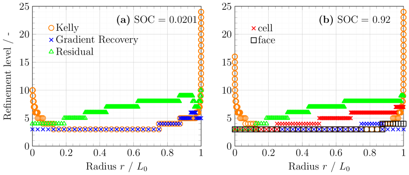
Figure 5: Same situation as in Figure 4(c)-(d), but with updated version of the residual based error estimator with $\gamma_{1}=0.001$ and $\gamma_{2}=1.0$.

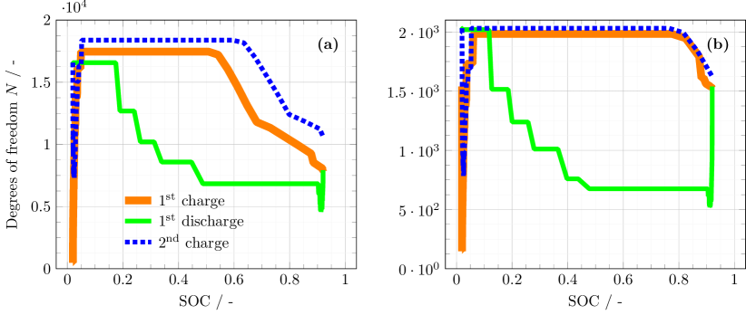
Figure 6: Number of DOFs over SOC for the residual based error estimator with $\gamma_{1}=1.0$ and $\gamma_{2}=1.0$ in (a) and updated version with $\gamma_{1}=0.001$ and $\gamma_{2}=1.0$ in (b).

It is known in literature that the edge fraction is the dominating one and the more important one for the error estimation, see for example Carstensen and Verfürth [1999] and [Verfürth, 2013, Section 1.6]. Therefore, we have additionally performed some simulations with an updated version of the residual based error estimator with $\gamma_{1}=0.001$ and $\gamma_{2}=1.0$. The smaller fraction of the cell error clearly reduces the refinement level of the residual based refinement strategy, comparing Figure 5(a)-(b) to Figure 4(c)-(d).

This influence of the cell error fraction is further investigated in Figure 6, where the number of degrees of freedom (DOFs) $(2+d)N$ is plotted for the residual based error estimator with $\gamma_{1}=1.0$ and $\gamma_{2}=1.0$. in Subfigure (a) and the updated version with $\gamma_{1}=0.001$ and $\gamma_{2}=1.0$ in Subfigure (b). Both plots show some qualitative similarities, which are the steep increase of the number of DOFs after the start of the first lithiation followed by some plateau and a decrease in the end of the first charge. The first discharge looks also similar, since the number of DOFs gets smaller but reaches a higher level at the end of the first discharge. For the second charge, there is the same behavior in both plots visible featuring a large drop in the number of DOFs and following then the same way as the first charge. However, there is one difference: the absolute number of DOFs is reduced by a factor of $10$ in the updated version. This shows again the significant influence of the cell error fraction.

Table 1: Error between the numerical solution compared to a highly resolved numerical solution regarding the respective norm: $\|\vec{y}-\vec{y}_{\text{highly\_resolved}}\|_{\square}$.

Error estimator	DOFs	$L^{2}\text{-Norm}$	$H^{1}\text{-Norm}$
Gradient recovery	$111$	$1.20\text{\times}{10}^{-06}$	$3.02\text{\times}{10}^{-06}$
Residual	$15\,939$	$3.08\text{\times}{10}^{-07}$	$1.07\text{\times}{10}^{-06}$
Residual updated	$1575$	$5.44\text{\times}{10}^{-07}$	$1.65\text{\times}{10}^{-06}$

In Table 1, we display the $L^{2}\text{-Norm}$ and $H^{1}\text{-Norm}$ of the numerical solution $\vec{y}$ compared with a highly resolved solution $\vec{y}_{\text{highly\_resolved}}$ at time $t=0.2~{}$\mathrm{h}$$. For the numerical results of the table, we use the exact computation of the Newton matrix and no AD. The high resolved solution is computed with $N=1.5$ million DOFs and updated $\operatorname{RelTol}_{t}=$1\text{\times}{10}^{-11}$$ and $\operatorname{AbsTol}_{t}=$1\text{\times}{10}^{-14}$$. The numerical solution $\vec{y}$ is computed with $\operatorname{RelTol}_{t}=$1\text{\times}{10}^{-7}$$, $\operatorname{AbsTol}_{t}=$1\text{\times}{10}^{-10}$$, initial time step size $\tau_{0}=$1\text{\times}{10}^{-10}$$ and initial refinement level with 17. We compare the results of the gradient recovery-, the residual based- and the updated residual based error estimator. On the one hand, it can be seen that the gradient recovery displays the lowest number of DOFs but also the largest errors. On the other hand, residual based methods feature smaller norm errors but have also significant larger number of DOFs. Interestingly, the updated case leads to a factor of ten fewer number of DOFs, whereas the error norms are at a comparable level. From this, we can conclude that it is more efficient to use the updated version of the residual based error estimator due to the smaller number of DOFs. Further, we are accurate enough with the updated version and do not need to solve the numerical simulations for the solutions with the higher number of DOFs.

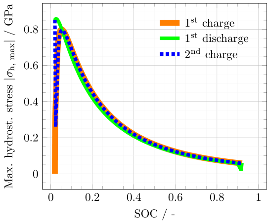
Figure 7: Absolute value of the maximal hydrostatic Cauchy stress $\sigma_{\text{h, max}}$ over SOC for charging–discharging–charging cycle for the residual based error estimator with updated constants $\gamma_{1}=0.001$ and $\gamma_{2}=1.0$.

Figure 7 displays the development of the absolute value of the maximal hydrostatic stress $\sigma_{\text{h}}$ over the particle radius during the three half cycles. The hydrostatic Cauchy stress is defined as $\sigma_{\text{h}}=(\sigma_{\text{r}}+2\sigma_{\phi})/3$ with the stress in radial direction $\sigma_{\text{r}}$ and in tangential direction $\sigma_{\phi}$. The evolution of the stress reveals high stresses at low SOC values and lower stresses at high SOC values. The increase of the first charge at low SOC results from the constant initial condition of the concentration. The small drop of the first discharge at high SOC and the large drop of the second charge at low SOC emerge from the change of stress curvature. For more information about this curvature change, see [Schoof et al., 2023a, Figure 7]. In total, it can be concluded from the SOC ranges and the behavior of the number of DOFs of Figure 6 and Figure 7 that for the 1D spherical symmetric case larger maximal Cauchy stress values are related with a larger number of DOFs.

Example 2: 2D Quarter Ellipse.

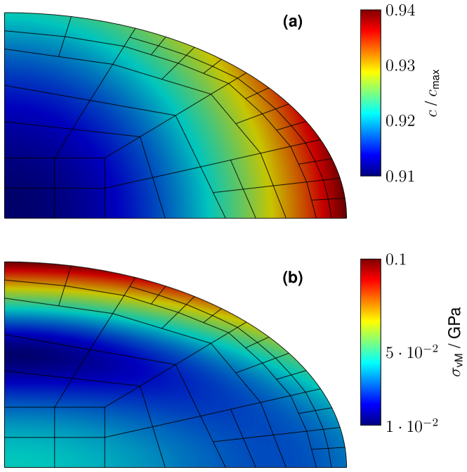
Figure 8: Numerical solution of the concentration $c$ in (a) and von Mises stress $\sigma_{\text{vM}}$ in (b) with the used mesh at the final simulation time $t_{\text{end}}=0.9~{}$\mathrm{h}$$ for the updated version of the residual based error estimator with $\gamma_{1}=0.001$ and $\gamma_{2}=1.0$.

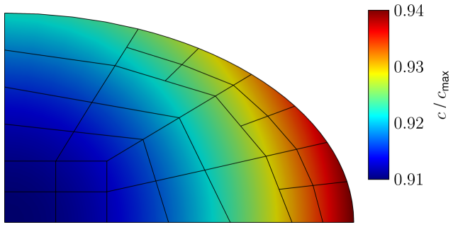
Figure 9: Numerical solution of the concentration $c$ with the used mesh at the final simulation time $t_{\text{end}}=0.9~{}$\mathrm{h}$$ with the gradient recovery estimator.

The 2D computational domain is a proof of concept to show the feasibility of the gradient recovery estimator and updated version of the residual based error estimator as adaptive refinement strategies. For the simulations, we have modified some parameters in the following way: the number of initial refinements to 6, initial time step size to $1\text{\times}{10}^{-8}$ and $t_{\text{end}}=0.9$. In Figure 8, the numerical solution of the concentration $c$ in Subfigure (a) and of the von Mises stress $\sigma_{\text{vM}}=\sqrt{\sigma_{11}^{2}+\sigma_{22}^{2}-\sigma_{11}\sigma_{22}+3\sigma_{12}^{2}}$ in Subfigure (b) are shown with the underlying mesh of the updated version of the residual based error estimator with $\gamma_{1}=0.001$ and $\gamma_{2}=1.0$. Due to the elliptical domain, more lithium gets inside or out of the host particle at the area with the highest surface to volume ratio which is at the particle surface of the larger half axis [Huttin, 2014, Section 2.2.3]. We point out that the mesh has higher refinements at areas of higher concentration values although the highest stresses are at the particle surface of the smaller half axis. The large von Mises stress $\sigma_{\text{vM}}$ at the smaller half axis occurs due to the forced zero stress in normal direction and the large tangential stresses in this area. This indicates that the concentration $c$ has a larger influence than the von Mises stress $\sigma_{\text{vM}}$ on the spatial mesh strategy in the two-dimensional distribution at one time step.

The numerical solution of the concentration $c$ with the underlying mesh of the gradient recovery refinement strategy is displayed in Figure 9. Here, also a less refined mesh fulfills the tolerances of the adaptive solution algorithm compared to the updated version of the residual based strategy. This is similar to the findings of the 1D spherical symmetric case.

5 Conclusion and Outlook

Conclusion. In this work, three different spatial refinement strategies are investigated which have been applied to a chemo-elastic model for Li-diffusion within aSi particles. The ready to use Kelly error estimator Arndt et al. [2023] of deal.II, the gradient recovery estimator of Castelli et al. [2021] and a residual based error estimator are compared. For the usage of the residual based error estimator, the strong formulation of the residual is derived explicitly in Section 2 including many dependencies of our chemo-mechanical coupled model approach. In Section 4, we considered the numerical results for a 3D spherical domain, reduced to 1D computational domain, and a 3D elliptical nanowire, reduced to 2D computational domain. For the 1D computational domain, we found out that the Kelly error estimator over-estimates the error at the boundary and therefore can not recommended for our application case. The gradient recovery estimator features higher refinement levels during the change of the lithium flux and rather lower refinement levels during solely the Li-diffusion periods. The residual based error estimator shows a stair-like behavior from the particle center to the particle surface. However, the cell error part leads to significant larger refinement levels compared to the face error part. Therefore, we have introduced an updated residual based error estimator with $\gamma_{1}=0.001$ and $\gamma_{2}=1.0$, which reduces the influence of the cell error part. The updated version leads to a more efficient error estimator, since the number of DOFs is smaller by a factor of $10$ and the updated error estimator results in a comparable $L^{2}$- and $H^{1}$-error compared to the residual case with $\gamma_{1}=1.0$ and $\gamma_{2}=1.0$.

During a charging and discharging process, higher Cauchy stress values are related with a higher number of DOFs, whereas in the 2D computational domain, the distribution of Li-concentration has a larger influence on the mesh distribution compared to the Cauchy stress distribution at one specific time step.

Outlook. Since we pointed out the significant influence of the cell error fraction of the residual based error estimator, further work is required for the calibration of the ratio of the cell and face errors of the residual based error estimator. However, as charging and discharging is a highly dynamic process, a suitable calibration should be carefully checked. Another application of great interest is the consideration of another definition of the elastic strain tensor $\mathsf{E}_{\text{el}}$ as in Schoof et al. [2023b] leading to an easy usage for further elasto-plastic couplings. In addition, the investigation of other battery active materials like graphite-silicon composites or materials for sodium-ion batteries is possible. Other 2D geometries and 3D geometries could also be taken into account.

Declaration of competing interest

The authors declare that they have no known competing financial interests or personal relationships that could have appeared to influence the work in this paper.

CrediT authorship contribution statement

R. Schoof: Conceptualization, Data curation, Formal Analysis, Investigation, Methodology, Software, Validation, Visualization, Writing – original draft L. Flür: Formal Analysis, Methodology, Software, Visualization, Writing – review & editing F. Tuschner: Data curation, Writing – review & editing W. Dörfler: Conceptualization, Funding acquisition, Project administration, Resources, Supervision, Writing – review & editing

Declaration of Competing Interest

The authors declare that they have no known competing financial interests or personal relationships that could have appeared to influence the work in this paper.

Data Availability Statement

Data will be made available on request.

Keywords

adaptive finite element method, residual based error estimator, finite deformation, lithium-ion batteries, numerical simulation

Appendices

A Abbreviations and Symbols

Abbreviations
AD	automatic differentiation
aSi	amorphous silicon
$\mathrm{C}$-rate	charging rate
DAE	differential algebraic equation
DOF	degree of freedom
NDF	numerical differentiation formula
OCV	open-circuit voltage
pmv	partial molar volume
SOC	state of charge

Symbol	Description
Latin symbols
$c$	concentration
$\mathsf{C}_{\text{el}}$	right Cauchy-Green tensor
$\bm{\mathds{C}}$	fourth-order stiffness tensor
$E$	Young’s modulus
$\mathsf{E}_{\text{el}}$	elastic strain tensor
$\mathsf{F}$	deformation gradient
$\mathsf{F}=\mathsf{F}_{\text{ch}}\mathsf{F}_{\text{el}}$	multiplicative decomposition of $\mathsf{F}$
$\mathsf{F}_{\text{ch}}$	chemical deformation gradient
$\mathsf{F}_{\text{el}}$	elastic deformation gradient
$\mathrm{Fa}$	Faraday constant
$G$	shear modulus / second Lamé constant
$\mathsf{Id}$	identity tensor
$J=J_{\text{ch}}J_{\text{el}}$	multiplicative decomposition of volume change
$k_{n}$	order of time integration algorithm at time $t_{n}$
${m}$	scalar valued mobility
$\vec{n}$, $\vec{n}_{0}$	normal vector on $\Omega$, $\Omega_{0}$
$\vec{N}$	lithium flux
${N}_{\text{ext}}$	external lithium flux
$\mathsf{P}$	first Piola–Kirchhoff stress tensor
$t$	time
$t_{n}$	time step
$t_{\text{cycle}}$	cycle time
$U_{\text{OCV}}$	OCV curve
$\vec{u}=\vec{x}-\vec{X}_{0}$	time dependent displacement vector
$v_{\text{pmv}}$	partial molar volume of lithium
$\vec{x}$	position in Eulerian domain
$\vec{X}_{0}$	initial placement
Greek symbols
$\gamma_{1}$	factor for the cell error of the residual based error estimator
$\gamma_{2}$	factor for the face error of the residual based error estimator
$\Gamma_{\text{in}}$	inner artificial boundary part
$\lambda$	first Lamé constant
$\lambda_{\text{ch}}$	factor of concentration induced deformation gradient
$\mu$	chemical potential
$\nu$	Poisson’s ratio
$\Omega$	Eulerian domain
$\Omega_{0}$	Lagrangian domain
$\psi=\psi_{\text{ch}}+\psi_{\text{el}}$	total energy
$\psi_{\text{ch}}$	chemical part of energy
$\psi_{\text{el}}$	elastic part of energy
$\rho$	density
$\mathsf{\sigma}$	Cauchy stress tensor
$\tau_{n}$	time step size at time $t_{n}$
Mathematical symbols
$\partial\Omega_{0}$	boundary of $\Omega_{0}$
$\bm{\nabla}_{0}$	gradient vector in Lagrangian domain
$\square\!:\!\tilde{\square}$	reduction of two dimensions of two tensors $\square$ and $\tilde{\square}$
$\bm{\mathcal{A}}[\mathsf{B}]$	reduction of the last two dimensions of the third order tensor $\bm{\mathcal{A}}$ and the second order tensor $\mathsf{B}$
$\bm{\mathds{A}}[\mathsf{B}]$	reduction of the last two dimensions of the fourth order tensor $\bm{\mathds{A}}$ and the second order tensor $\mathsf{B}$
$\partial_{\square}$	partial derivative with respect to $\square$
Indices
${\square}_{0}$	considering variable in Lagrangian domain or initial condition
${\square}_{\text{ch}}$	chemical part of $\square$
${\square}_{\text{com}}$	computational part of $\square$
${\square}_{\text{el}}$	elastic part of $\square$
${\square}_{\text{max}}$	maximal part of $\square$
${\square}_{\text{min}}$	minimal part of $\square$

B Simulation Parameters

The dimensionless variables of the considered model equations are given in Table 4 and the used model parameters for the numerical simulations are listed in Table 5.

Table 4: Dimensionless variables of the used model equations.

$\tilde{\vec{X}}_{0}=\vec{X}_{0}/L_{0}$	$\tilde{t}=t/t_{\text{cycle}}$	$\tilde{\vec{u}}=\vec{u}/L_{0}$	$\tilde{c}=c/c_{\max}$	$\tilde{v}_{\text{pmv}}={v}_{\text{pmv}}c_{\max}$
$\tilde{\rho\psi}=\rho\psi/R_{\text{gas}}Tc_{\max}$		$\tilde{\mu}=\mu/R_{\text{gas}}T$	$\tilde{E}=E/R_{\text{gas}}Tc_{\max}$
$\mathrm{Fo}=Dt_{\text{cycle}}/L_{0}^{2}$   $\tilde{N}_{\text{ext}}={N}_{\text{ext}}t_{\text{cycle}}/L_{0}c_{\max}$			$\tilde{U}_{\text{OCV}}=\mathrm{Fa}\,{U}_{\text{OCV}}/R_{\text{gas}}T$

Table 5: Model parameters for numerical experiments von Kolzenberg et al. [2022].

Description	Symbol	Value	Unit	Dimensionless
Universal gas constant	$R_{\text{gas}}$	$8.314$	$\mathrm{J}\text{\,}{\mathrm{mol}}^{-1}\text{\,}{\mathrm{K}}^{-1}$	$1$
Faraday constant	$\mathrm{Fa}$	$96485$	$\mathrm{J}\text{\,}{\mathrm{V}}^{-1}\text{\,}{\mathrm{mol}}^{-1}$	$1$
Operation temperature	$T$	$298.15$	$\mathrm{K}$	$1$
Silicon
Particle length scale	$L_{0}$	$50\text{\times}{10}^{-9}$	$\mathrm{m}$	1
Diffusion coefficient	$D$	$1\text{\times}{10}^{-17}$	${\mathrm{m}}^{2}\text{\,}{\mathrm{s}}^{-1}$	$14.4$
OCV curve	$U_{\text{OCV}}$	von Kolzenberg et al. [2022]	$\mathrm{V}$	von Kolzenberg et al. [2022]
Young’s modulus	$E$	$90.13\text{\times}{10}^{9}$	$\mathrm{Pa}$	$116.74$
Partial molar volume	$v_{\text{pmv}}$	$10.96\text{\times}{10}^{-6}$	${\mathrm{m}}^{3}\text{\,}{\mathrm{mol}}^{-1}$	$3.41$
Maximal concentration	$c_{\text{max}}$	$311.47\text{\times}{10}^{3}$	$\mathrm{mol}\text{\,}{\mathrm{m}}^{-3}$	$1$
Initial concentration	$c_{0}$	$6.23\text{\times}{10}^{3}$	$\mathrm{mol}\text{\,}{\mathrm{m}}^{-3}$	$2\text{\times}{10}^{-2}$
Poisson’s ratio	$\nu$	$0.22$	$\mathrm{-}$	$0.22$

References

• Writer [2019] B. Writer. Lithium-Ion Batteries: A Machine-Generated Summary of Current Research. Springer International Publishing, Cham, 2019. doi:10.1007/978-3-030-16800-1.
• Armand et al. [2020] M. Armand, P. Axmann, D. Bresser, M. Copley, K. Edström, C. Ekberg, D. Guyomard, B. Lestriez, P. Novák, M. Petranikova, W. Porcher, S. Trabesinger, M. Wohlfahrt-Mehrens, and H. Zhang. Lithium-ion batteries – current state of the art and anticipated developments. J. Power Sources, 479:228708, 2020. doi:10.1016/j.jpowsour.2020.228708.
• Xu et al. [2023] J. Xu, X. Cai, S. Cai, Y. Shao, C. Hu, S. Lu, and S. Ding. High-energy lithium-ion batteries: Recent progress and a promising future in applications. Energy Environ. Mater., 6(5), 2023. doi:10.1002/eem2.12450.
• Zhan et al. [2021] R. Zhan, X. Wang, Z. Chen, Z. W. Seh, L. Wang, and Y. Sun. Promises and challenges of the practical implementation of prelithiation in lithium-ion batteries. Adv. Energy Mater., 11(35), 2021. doi:10.1002/aenm.202101565.
• Martí-Florences et al. [2023] M. Martí-Florences, A. Cecilia, and R. Costa-Castelló. Modelling and estimation in lithium-ion batteries: A literature review. Energies, 16(19):6846, 2023. doi:10.3390/en16196846.
• Nzereogu et al. [2022] P. U. Nzereogu, A. D. Omah, F. I. Ezema, E. I. Iwuoha, and A. C. Nwanya. Anode materials for lithium-ion batteries: A review. Appl. Surf. Sci. Adv., 9:100233, 2022. doi:10.1016/j.apsadv.2022.100233.
• Zhao et al. [2019] Y. Zhao, P. Stein, Y. Bai, M. Al-Siraj, Y. Yang, and B.-X. Xu. A review on modeling of electro-chemo-mechanics in lithium-ion batteries. J. Power Sources, 413:259–283, 2019. doi:10.1016/j.jpowsour.2018.12.011.
• Zuo et al. [2017] X. Zuo, J. Zhu, P. Müller-Buschbaum, and Y. Cheng. Silicon based lithium-ion battery anodes: A chronicle perspective review. Nano Energy, 31:113–143, 2017. doi:10.1016/j.nanoen.2016.11.013.
• Tomaszewska et al. [2019] A. Tomaszewska, Z. Chu, X. Feng, S. O’Kane, X. Liu, J. Chen, C. Ji, E. Endler, R. Li, L. Liu, Y. Li, S. Zheng, S. Vetterlein, M. Gao, J. Du, M. Parkes, M. Ouyang, M. Marinescu, G. Offer, and B. Wu. Lithium-ion battery fast charging: A review. eTransportation, 1:100011, 2019. doi:10.1016/j.etran.2019.100011.
• Li et al. [2021] P. Li, H. Kim, S.-T. Myung, and Y.-K. Sun. Diverting exploration of silicon anode into practical way: A review focused on silicon-graphite composite for lithium ion batteries. Energy Stor. Mater., 35:550–576, 2021. doi:10.1016/j.ensm.2020.11.028.
• Tian et al. [2015] H. Tian, F. Xin, X. Wang, W. He, and W. Han. High capacity group-IV elements (Si, Ge, Sn) based anodes for lithium-ion batteries. J. Materiomics, 1(3):153–169, 2015. doi:10.1016/j.jmat.2015.06.002.
• Zhang [2011] W.-J. Zhang. A review of the electrochemical performance of alloy anodes for lithium-ion batteries. J. Power Sources, 196(1):13–24, 2011. doi:10.1016/j.jpowsour.2010.07.020.
• Miranda et al. [2016] D. Miranda, C. M. Costa, A. M. Almeida, and S. S. Lanceros-Méndez. Computer simulations of the influence of geometry in the performance of conventional and unconventional lithium-ion batteries. Appl. Energy, 165:318–328, 2016. doi:https://doi.org/10.1016/j.apenergy.2015.12.068.
• Xu and Zhao [2016] R. Xu and K. Zhao. Electrochemomechanics of Electrodes in Li-Ion Batteries: A Review. Journal of Electrochemical Energy Conversion and Storage, 13(3):030803, 2016. doi:10.1115/1.4035310.
• Abu et al. [2023] S. M. Abu, M. A. Hannan, M. S. Hossain Lipu, M. Mannan, P. J. Ker, M. J. Hossain, and T. M. Indra Mahlia. State of the art of lithium-ion battery material potentials: An analytical evaluations, issues and future research directions. J. Clean. Prod., 394:136246, 2023. doi:10.1016/j.jclepro.2023.136246.
• Korthauer [2018] R. Korthauer. Lithium-Ion Batteries: Basics and Applications. Springer Berlin Heidelberg, 2018. doi:10.1007/978-3-662-53071-9.
• Castelli et al. [2021] G. F. Castelli, L. von Kolzenberg, B. Horstmann, A. Latz, and W. Dörfler. Efficient simulation of chemical-mechanical coupling in battery active particles. Energy Technol., 9(6):2000835, 2021. doi:10.1002/ente.202000835.
• Di Leo et al. [2014] C. V. Di Leo, E. Rejovitzky, and L. Anand. A Cahn–Hilliard-type phase-field theory for species diffusion coupled with large elastic deformations: application to phase-separating li-ion electrode materials. J. Mech. Phys. Solids, 70:1–29, 2014. doi:10.1016/j.jmps.2014.05.001.
• Kelly et al. [1983] D. W. Kelly, J. P. de S. R. Gago, O. C. Zienkiewicz, and I. Babuška. A posteriori error analysis and adaptive processes in the finite element method. I. Error analysis. Internat. J. Numer. Methods Engrg., 19(11):1593–1619, 1983. doi:10.1002/nme.1620191103.
• Arndt et al. [2023] D. Arndt, W. Bangerth, M. Bergbauer, M. Feder, M. Fehling, J. Heinz, T. Heister, L. Heltai, M. Kronbichler, M. Maier, P. Munch, J-.P. Pelteret, B. Turcksin, D. Wells, and S. Zampini. The deal. II library, version 9.5. J. Numer. Math., 31(3):231–246, 2023. doi:10.1515/jnma-2023-0089.
• Ainsworth and Oden [2000] M. Ainsworth and J. T. Oden. A Posteriori Error Estimation in Finite Element Analysis. Pure and Applied Mathematics. John Wiley & Sons, Inc., New York, 2000. doi:10.1002/9781118032824.
• Brenner and Scott [2008] S. C. Brenner and L. R. Scott. The Mathematical Theory of Finite Element Methods. Springer New York, 2008. doi:10.1007/978-0-387-75934-0.
• Babuška and Gatica [2010] I. Babuška and G. N. Gatica. A residual-based a posteriori error estimator for the Stokes-Darcy coupled problem. SIAM J. Numer. Anal., 48(2):498–523, 2010. doi:10.1137/080727646.
• Ainsworth and Oden [1997] M. Ainsworth and J. T. Oden. A posteriori error estimation in finite element analysis. Comput. Methods Appl. Mech. Engrg., 142(1-2):1–88, 1997. doi:10.1016/S0045-7825(96)01107-3.
• Verfürth [1996] R. Verfürth. A review of a posteriori error estimation and adaptive mesh-refinement techniques. Wiley-Teubner series in advances in numerical mathematics. Wiley [u.a.], Chichester, 1996.
• Carstensen and Klose [2003] C. Carstensen and R. Klose. A posteriori finite element error control for the $p$-Laplace problem. SIAM J. Sci. Comput., 25(3):792–814, 2003. doi:10.1137/S1064827502416617.
• Schoof et al. [2022] R. Schoof, G. F. Castelli, and W. Dörfler. Parallelization of a finite element solver for chemo-mechanical coupled anode and cathode particles in lithium-ion batteries. In T. Kvamsdal, K. M. Mathisen, K.-A. Lie, and M. G. Larson, editors, 8th European Congress on Computational Methods in Applied Sciences and Engineering (ECCOMAS Congress 2022), Barcelona, 2022. CIMNE. doi:10.23967/eccomas.2022.106.
• Schoof et al. [2023a] R. Schoof, G. F. Castelli, and W. Dörfler. Simulation of the deformation for cycling chemo-mechanically coupled battery active particles with mechanical constraints. Comput. Math. Appl., 149:135–149, 2023a. doi:10.1016/j.camwa.2023.08.027.
• von Kolzenberg et al. [2022] L. von Kolzenberg, A. Latz, and B. Horstmann. Chemo-mechanical model of sei growth on silicon electrode particles. Batter. Supercaps, 5(2):e202100216, 2022. doi:10.1002/batt.202100216.
• Holzapfel [2010] G. A. Holzapfel. Nonlinear Solid Mechanics. John Wiley & Sons, Ltd., Chichester, 2010.
• Braess [2007] D. Braess. Finite Elements. Cambridge University Press, Cambridge, third edition, 2007. doi:10.1007/978-3-540-72450-6.
• Latz and Zausch [2015] A. Latz and J. Zausch. Multiscale modeling of lithium ion batteries: thermal aspects. Beilstein J. Nanotechnol., 6:987–1007, 2015. doi:10.3762/bjnano.6.102.
• Latz and Zausch [2011] A. Latz and J. Zausch. Thermodynamic consistent transport theory of Li-ion batteries. J. Power Sources, 196(6):3296–3302, 2011. doi:10.1016/j.jpowsour.2010.11.088.
• Schammer et al. [2021] M. Schammer, B. Horstmann, and A. Latz. Theory of transport in highly concentrated electrolytes. J. Electrochem. Soc., 168(2):026511, 2021. doi:10.1149/1945-7111/abdddf.
• Chan et al. [2007] C. K. Chan, H. Peng, G. Liu, K. McIlwrath, X. F. Zhang, R. A. Huggins, and Y. Cui. High-performance lithium battery anodes using silicon nanowires. Nat. Nanotechnol., 3(1):31–35, 2007. doi:10.1038/nnano.2007.411.
• Keil et al. [2016] P. Keil, S. F. Schuster, J. Wilhelm, J. Travi, A. Hauser, R. C. Karl, and A. Jossen. Calendar aging of lithium-ion batteries. J. Electrochem. Soc., 163(9):A1872–A1880, 2016. doi:10.1149/2.0411609jes.
• Latz and Zausch [2013] A. Latz and J. Zausch. Thermodynamic derivation of a Butler–Volmer model for intercalation in Li-ion batteries. Electrochim. Acta, 110:358–362, 2013. doi:10.1016/j.electacta.2013.06.043.
• Lubliner [2006] J. Lubliner. Plasticity theory. Pearson Education, Inc., New York, 2006. doi:10.1115/1.2899459.
• Deng [2015] D. Deng. Li-ion batteries: basics, progress, and challenges. Energy Sci. Eng., 3(5):385–418, 2015. doi:10.1002/ese3.95.
• Piller et al. [2001] S. Piller, M. Perrin, and A. Jossen. Methods for state-of-charge determination and their applications. J. Power Sources, 96(1):113–120, 2001. doi:10.1016/s0378-7753(01)00560-2.
• Reichelt et al. [1997] M. W. Reichelt, L. F. Shampine, and J. Kierzenka. Matlab ode15s, 1997. URL http://www.mathworks.com. Copyright 1984–2020 The MathWorks, Inc.
• Shampine and Reichelt [1997] L. F. Shampine and M. W. Reichelt. The MATLAB ODE suite. SIAM J. Sci. Comput., 18(1):1–22, 1997. doi:10.1137/S1064827594276424.
• Shampine et al. [1999] L. F. Shampine, M. W. Reichelt, and J. A. Kierzenka. Solving index-$1$ DAEs in MATLAB and Simulink. SIAM Rev., 41(3):538–552, 1999. doi:10.1137/S003614459933425X.
• Shampine et al. [2003] L. F. Shampine, I. Gladwell, and S. Thompson. Solving ODEs with MATLAB. Cambridge University Press, Cambridge, 2003. doi:10.1017/CBO9780511615542.
• Schoof et al. [2023b] R. Schoof, J. Niermann, A. Dyck, T. Böhlke, and W. Dörfler. Efficient modeling and simulation of chemo-elasto-plastically coupled battery active particles. Comput. Mech., 2023b. doi:10.48550/arXiv.2310.05440.
• Castelli [2021] G. F. Castelli. Numerical Investigation of Cahn–Hilliard-Type Phase-Field Models for Battery Active Particles. PhD thesis, Karlsruhe Institute of Technology (KIT), 2021.
• Trilinos Project Team [2023] The Trilinos Project Team. The Trilinos Project Website, 2023. URL https://trilinos.github.io.
• Davis [2004] T. A. Davis. Algorithm 832: UMFPACK V4.3—an unsymmetric-pattern multifrontal method. ACM Trans. Math. Software, 30(2):196–199, 2004. doi:10.1145/992200.992206.
• bw HPC Team [2024] WIKI bw HPC Team. BwUniCluster 2.0 Hardware and Architecture, 2024. URL https://wiki.bwhpc.de/e/BwUniCluster_2.0_Hardware_and_Architecture.
• Carstensen and Verfürth [1999] C. Carstensen and R. Verfürth. Edge residuals dominate a posteriori error estimates for low order finite element methods. SIAM J. Numer. Anal., 36(5):1571–1587, 1999. doi:10.1137/S003614299732334X.
• Verfürth [2013] R. Verfürth. A posteriori error estimation techniques for finite element methods. Numerical mathematics and scientific computation. Oxford University Press, Oxford, 2013.
• Huttin [2014] M. Huttin. Phase-field modeling of the influence of mechanical stresses on charging and discharging processes in lithium ion batteries. PhD thesis, Karlsruher Institut für Technologie (KIT), Karlsruhe, 2014.