Interpreting deviations between AR-VTG and GR
Abstract
The Cosmic microwave background (CMB) anisotropies predicted by two cosmological models are compared, one of them is the standard model of general relativity with cold dark matter and cosmological constant, whereas the second model is based on a consistent vector-tensor theory of gravitation explaining solar system and cosmological observations. It is proved that the resulting differences -between the anisotropies of both models- are due to the so-called late integrated Sachs Wolfe effect and, consequently, cross correlations between maps of CMB temperatures and tracers of the dark matter distribution could be used in future to select one of the above models. The role of reionization is analysed in detail.
Keywords Modified theories of gravity; Cosmology: late integrated Sachs-Wolfe.
1 Introduction
In Ref. [1] an analysis of modified gravity theories, which takes in account current CMB data, was presented. As it is stated in this paper: "Those models which are close to are in broad agreement with current constraints on the background cosmology, but the perturbations may still evolve differently and hence it is important to test their predictions against CMB data". In agreement with these comments, present paper studies the case of another successfully modified gravity theory that is close to the model.
Any vector-tensor gravity (VTG) theory involves the metric tensor and a vector field . These fields are coupled to build up an appropriate action leading to the basic equations via variational calculations.
There are many actions and VTG theories [2, 3] , here we focus our attention on one of these theories free from quantum ghosts and classical instabilities. It has the same parameterized post-Newtonian limit as general relativity (GR) and may explain cosmic microwave background (CMB) anisotropies as well as GR [4, 5, 6, 7] . In this vector-tensor theory, the outer metric corresponding to a spherically symmetric mass distribution has the same form as the well known Reissner-Nordström solution of Einstein-Maxwell equations [8] , whose source is a charged spherically symmetric mass distribution. This implies that, in the VTG theory (no charges), there are repulsive gravitational forces at stellar scales, just as it occurs in Einstein-Maxwell theory for a charged star. These forces might affect neutron star structure and the gravitational collapse (to be studied elsewhere). Moreover, there is also a gravitational cosmological repulsion as that due to the cosmological constant. On account of these facts, this theory shall from now on be called attractive-repulsive vector-tensor gravity (AR-VTG). As it was claimed in Ref. [7], it is convenient to mention that this theory is not a particular case of the Generalized Proca Theories (GPT) [9] , which also involve a vector field .
As it was discussed in Ref. [6], the CMB anisotropies produced at are expected to be identical in GR and AR-VTG; nevertheless, close to , some AR-VTG scalar cosmological modes (see mode definitions in Refs. [10, 11]), involved in the equations describing the evolution of the CMB photon distribution function (see Ref. [12]), begin to deviate from those of GR. These deviations might produce significant differences between the CMB anisotropies of GR and AR-VTG, but the redshift dependence of these differences requires numerical estimates which are performed below. Evidently, primary anisotropy is produced at and; consequently, the differences between GR and AR-VTG anisotropies at must be due to some kind of secondary anisotropy. At these low redshifts various effects are being produced: (i) the effect due to reionization (hereafter called R-effect), which is due to the interaction of free electrons with CMB photons via Thompson scattering, (ii) the so-called late integrated Sachs-Wolfe (LISW) effect due to large strictly linear scales, and (iii) the Rees-Sciama effect produced by smaller nonlinear scales.
The Rees-Sciama effect is too small to be detected [13] ; hence, we focus our attention on the R and the LISW effects [14, 15] . In GR, these effects may be estimated with the code CAMB [16] , whereas a new code (hereafter VTCAMB) has been specially designed -by us- to carry out the corresponding estimations in the context of AR-VTG (see Ref. [7]).
In this paper, , , , and stands for the gravitation constant, the scale factor, the conformal time, and the redshift, respectively. Our signature is (–,+,+,+). Greek indexes run from 0 to 3, while the latin ones from 1 to 3. Symbol () stands for a covariant (partial) derivative. Whatever the function may be, stands for the partial derivative with respect to the conformal time. The antisymmetric tensor is defined by the relation . It has nothing to do with the electromagnetic field. Quantities , , and are the covariant components of the Ricci tensor, the scalar curvature and the determinant of the matrix formed by the covariant components of the metric, respectively. Units are chosen in such a way that the speed of light, , takes on the value . Quantity , given in , is considered as a measure of CMB angular power spectra. This quantity and other ones depending on it are represented in various Figures.
This paper is structured as follows: The AR-VTG theory is summarized in Sect. 2. The origin of the deviations between GR and AR-VTG is analysed in Sect. 3, and the variation of these deviations with the redshift is studied in Sect.4. Finally, section 5 displays our main conclusions and an appropriate discussion.
2 AR-VTG foundations.
2.1 Generalities.
AR-VTG is particular parameterization of the general unconstrained VTG proposed by Will, Nordtvedt and Hellings [17, 18] in early 1970s. All these theories were based on the action [2]:
| (1) | |||||
where , , and are arbitrary parameters and is the matter Lagrangian density, which couples matter with the fields of the VTG theory.
There is a detailed analysis of the viability for VTG’s theories in Ref. [19] which determines the theories that may deserve our attention. This studio includes the calculation of the propagation speeds for the different perturbation modes and also the conditions for the absence of quantum ghosts. Regarding Ref. [19] the parameterization , , leaving arbitrary is a viable set of theories in terms of classical stability, local gravity constraints and absence of ghosts. Moreover the perturbations of mentioned model propagate at the speed of light which leads to the absence of classical unstable modes. AR-VTG theory is obtained when previous parameterization settings are applied to the general unconstrained VTG.
Let us now briefly summarize the AR-VTG basic equations, which were derived in Refs. [4, 5] from an appropriated action, which is a particularization of the general vector-tensor action given in Ref. [2]. The resulting field equations are:
| (2) |
| (3) |
where is the Einstein tensor, is the GR energy momentum tensor, with , and
| (4) | |||||
Equation (3) leads to the following conservation law
| (5) |
for the fictitious current . Moreover, the conservation laws and are satisfied by any solution of Eqs. (2) and (3).
The pair of parameters (, ) must satisfy the inequality to prevent the existence of quantum ghosts and unstable modes in AR-VTG (see Ref. [19]).
2.2 The background cosmology.
Let us now consider a flat uncharged homogeneous and isotropic background universe with matter and radiation where the isentropic uncharged perfect fluid is characterized by an energy density and a pressure (subscript B refers to background quantities). In this flat background using conformal time, the metric can be written in the form:
| (6) |
Furthermore, the covariant components of the vector field are and tensor vanish. On the other hand it is worthwhile to notice that the relation is satisfied (see Ref. [2]) so matter and radiation evolve as in the standard Friedmann-Robertson-Walker model of GR (immediately is obtained).
Taking into account , Eq. (3) leads to
| (7) |
and then the quantity is a constant and, consequently, tensor has the same form as the energy-momentum tensor corresponding to vacuum; namely, one has , where is the energy density due de vector field. This means that the resulting theory is equivalent to GR plus a cosmological constant. In terms of the component the equation (7) is
| (8) |
while equations 2 are
| (9) |
and
| (10) |
where
| (11) |
Hence the equation of state is , so due the energy density of the evolving field is constant, we can state that this field acts as a cosmological constant. Obviously the condition must be required to have a positive energy density in the background universe (see Ref. [6]); hence, taking into account the previous inequality , the inequalities must be satisfied.
The necessary initial values for the integration are obtained at high redshift during the radiation dominated era, where it’s found that and satisfy the above background field equations. At one finds:
| (12) |
Subscript "in" of previous quantities refers to initial values at .
2.3 The cosmological perturbations.
In order to describe cosmological perturbations, the formalism summarized in Ref. [10] (see also Ref. [11]) is used. In this formalism there are three types of perturbations whose evolution is independent during the linear regime: scalar, vector, and tensor fluctuations. There are no tensor modes involved in the expansion of the introduced vector field, so the existing ones satisfy the same equations as in GR. Formally the vector fluctuations are as in Einstein-Maxwell. The main reason lies in the fact that the action (1) is full equivalent to
| (13) |
for the parameterization , , and this action differs in essence, from the Einstein-Maxwell one, in the term proportional to , which is an scalar.
At linear level the vector perturbation of the vector field can be written , where are the vector harmonics which are a solution of the Helmholtz equation (see Ref. [10]), and is the wave number that sets the spatial scale of the perturbation. The evolution equation for the vector modes amplitude is [7]
| (14) |
It’s interesting realize that this mode is uncoupled from the rest of mode equations, so it has no impact on the evolution of the other modes.
Finally, all the scalar modes of GR are also involved in AR-VTG but, in order to describe the scalar modes associated to the field , we introduce a new gauge invariant scalar mode [5, 6] which is the first order term in the harmonic expansion of the scalar function defined as follows:
| (15) |
where the scalar harmonic is a solution of the Helmholtz equation (see Ref. [10]). There are no more independent AR-VTG scalar modes. From Eq. (7), following uncoupled differential equation for the new mode is obtained:
| (16) |
This equation just involves, apart from the new AR-VTG scalar mode and its derivatives, the background functions , and the wave number. It’s convenient to write scalar perturbation equations in the synchronous gauge and in terms of the scalar modes defined in Ref. [12], the reason is because those are the functions and gauge used by the original CAMB code and the modified one VTCAMB. There are just AR-VTG corrections terms to the standard GR in equations (21a)–(21c) derived in Ref. [12], this set of modified equations are:
| (17) |
| (18) |
| (19) |
where . In the above equations and are the scalar modes related with the metric while , and are the scalar modes related with fluid (density fluctuation, divergence of fluid velocity and the isotropic pressure perturbation, respectively). The same functions (without the tilde) and its definitions are found in Ref. [12], while the one can be located in Ref. [10]. The rest of scalar modes equations remain unaltered (see Eqs. (92) and subsequent in paper Ref. [12]).
As in previous subsection, initial conditions equations for the AR-VTG scalar modes at redshift in the radiation dominated era, are obtained. In GR the initial conditions equations involve a normalization constant named at Ref. [12] while in AR-VTG it involves an extra one we call , that is related with the initial spectrum of the new scalar mode in the following manner: . The complete set of modified initial conditions equations can be found in Ref. [7] labelled as (2.23).
3 CMB anisotropy differences between GR and AR-VTG.
3.1 Numerical computational fitting.
In order to fit observational data with the model predictions an adapted and modified version of the standard well known codes COSMOMC [21] (hereafter VTCOSMOMC) and CAMB have been used. There are a lot of tasks related with the adaptation and modifications of the codes as the inclusion of the background and scalar modes extra field equations, and its corresponding initial conditions equations, the modification of the scalar modes equations including the new terms and again its modified corresponding initial conditions equations. But this is not enough, the introduction of the new parameter implies changes at original COSMOMC (the Markov sample chains generator software) code, modifications related with the integration steps in wave number and in time, numerical issues and other technical concerns.
As related in the above subsection there is a new constant whose absolute value normalizes the spectrum of the vector field (its divergence) scalar cosmological perturbations. This is the new parameter that has been added in the different fitting calculations. Apart of the mentioned above, we include six GR parameters to conform a minimal base model to fit, those parameters are: , , , , , and , where and are the density parameters of baryons and dark matter, respectively, is the reduced Hubble constant, is the reionization optical depth, is the spectral index of the power spectrum of scalar modes, and is the normalization constant of the same spectrum whose form is , finally, the parameter (angular acoustic scale) is defined by the relation , where is the sound horizon at decoupling redshift , and is the angular diameter distance at the same redshift. This minimal base model is expanded for some cases when tensor modes are included, in such a case, following additional parameters are considered: (the primordial tensor to scalar initial amplitude at the pivot scale of ), and (running index).
| Parameter | Best Fit | 68 Lower Limit | 68 Upper Limit |
|---|---|---|---|
| 1.596 | -2.149 | 2.149 | |
| 0.02216 | 0.02179 | 0.02235 | |
| 0.1187 | 0.1169 | 0.1222 | |
| 0.0893 | 0.0749 | 0.1013 | |
| 0.9657 | 0.9535 | 0.9684 | |
| 3.085 | 3.060 | 3.110 | |
| 1.0411 | 1.0407 | 1.0419 |
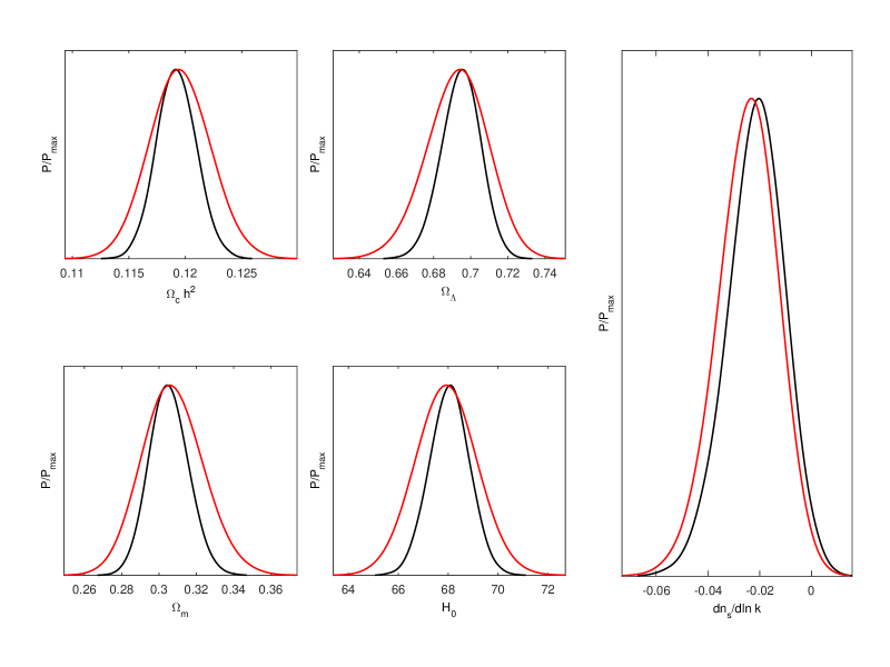
A variety combination of evidence sources that includes Ia supernovae (SNIa), WMAP 7 years CMB anisotropies (WP7), Planck CMB anisotropies (Planck), WMAP polarization anisotropy at low (WP), baryon acoustic oscillations (BAO), have been used. A complete analysis of the results can be found at Ref. [6] and Ref. [7], however let us summarize useful obtained information for the current studio. When the constant is considered as an additional parameter to be adjusted and a certain confidence level is assumed, we have found that, in AR-VTG fitting calculations, most GR parameters belong to intervals wider than those of the GR fitting calculations and, consistently, quantity takes on non-vanishing values. As a sample see Fig. 1 where the left four panels represent the normalized likelihood for different standard GR parameters (the best fit values, including the 68 confidence intervals can be found at Table 1); at the stretched right panel the normalized likelihood function for the running index parameter, when tensor modes are included, is presented. This is a pattern that is repeated when using different evidence data sources combinations and strongly suggests that a parameter facilitates the adjustments between predictions and cosmological observations.
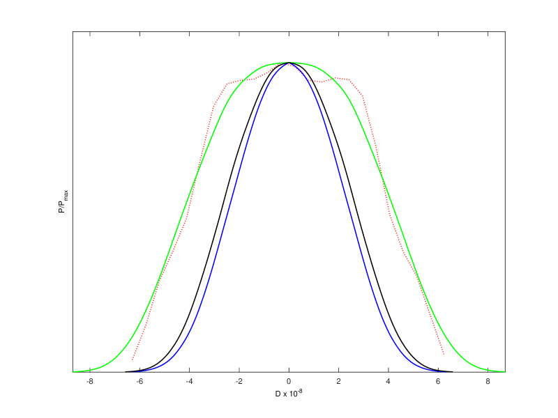
Parameter plays a positive statistical role in the study of AR-VTG scalar perturbations. Depending on the set of evidence sources considered and the inclusion or not of tensor fluctuations (and the parameters related with it), different intervals for the confidence level of (68), (95), and (99.7) are achieved. The Fig. 2 represents a summary of mentioned results, for instance at confidence level those are: for just scalar perturbations and Planck + WP, same as previous one but including BAO, and when including tensor modes with running index and using Planck + WP as evidence sources.
3.2 On the CMB anisotropy differences.
Let us now describe the method used to analyse the origin of the CMB anisotropy differences between GR and AR-VTG.
Codes CAMB and VTCAMB are used to estimate the R and LISW effects at . Reionization is modelled by using the standard optical depth parameter.
In any case, results from CAMB based on a minimal six parameters fit model are compared with the results obtained with VTCAMB for the same values of the six parameters plus a new parameter characteristic of AR-VTG. This parameter labelled will take on the value , which was proved to be compatible with CMB observations at the confidence level (see previous subsection and Ref. [7]).
We use two sets of six parameters obtained in previous papers -in the context of GR- to fit theoretical predictions and observations. These sets are hereafter called and . The six parameter values for () are given in the first (second) data row of Table 2.
| Parameters | ||||||
|---|---|---|---|---|---|---|
| 0.02209 | 0.1195 | 0.0927 | 0.9633 | 3.093 | 1.0415 | |
| 0.02227 | 0.1184 | 0.067 | 0.9681 | 3.064 | 1.04106 |
Five of the six parameters given by CAMB -in the GR context- take on similar values whatever the observational data may be (WMAP, PLANCK, and so on); however, parameter depends on the CMB polarization data used in fit calculations. The parameter values –obtained in Ref. [7]– were derived by using Planck data about the CMB temperature distribution, plus WMAP data on CMB polarization anisotropy at low , and the resulting is close to 0.093 (first data row of Table 2); nevertheless, the parameter values, given in the second data row of Table 2, were derived in Ref. [20] by using both temperature and polarization Planck data (see column 3 of Table 4 in this last reference); in this second case, the parameter value is close to 0.067; namely, this parameter is rather smaller than that of the fit, which is a consequence of important differences in the polarization data. Both fits have been performed by using CAMB and COSMOMC codes. December 2013 (November 2015) versions were used to get the () parameter values.
As it has been stated in Sect. 1, the differences between the CMB anisotropies of GR and AR-VTG must be due to a combination of the R and LISW effects at . Reionization contributes to the LISW effect [14] (-effect) and, moreover, it also creates anisotropy due to path mixing, Doppler effects due to motions in the reionization electron distribution, and so on (-effect). Our main goal is to disentangle the , , and LISW contributions to find out the nature of the aforementioned differences. Since there are well defined terms giving the LISW effect -in CAMB and VTCAMB- and these terms include reionization contributions (-effect), we can proceed as follows:
-
i
Once a data row of Table 2 has been selected and the value has been fixed, Codes CAMB and VTCAMB may be used to calculate the total numbers in GR and AR-VTG, respectively.
-
ii
For the same parameters, the LISW contribution to the quantities may be easily calculated. This computation may be performed by integrating, from redshift to , only the terms giving the LISW effect (including ); namely, by canceling any other contribution to the CMB angular power spectrum, including reionization effects (not contained in LISW); in this way, only the reionization contribution, , to the LISW effect is taken into account.
Results obtained with this procedure may be used to calculate, for the chosen parameters, both absolute and relative deviations between the GR and AR-VTG angular power spectra. These deviations may be estimated for the total quantities, and also for the LISW contribution to the angular power spectrum. The absolute deviations are , whereas the relative ones are . These deviations are presented in Figs. 3 to 6.
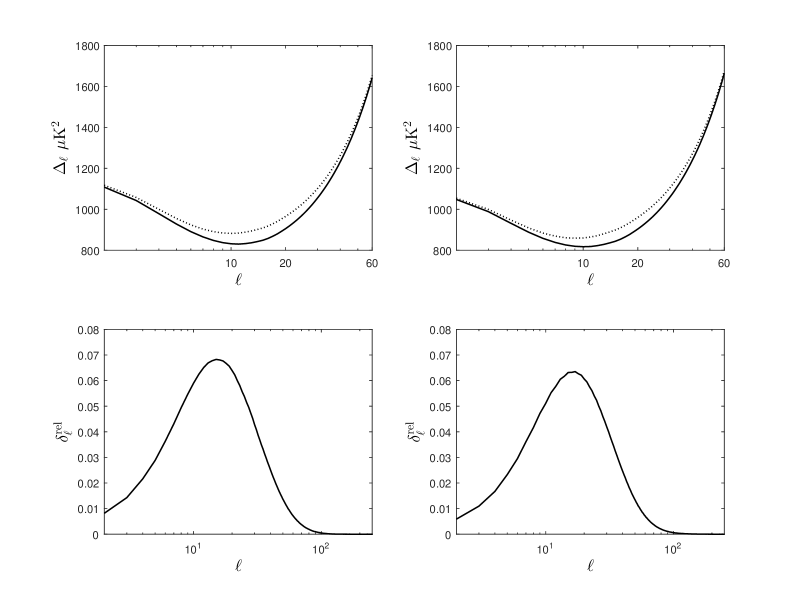
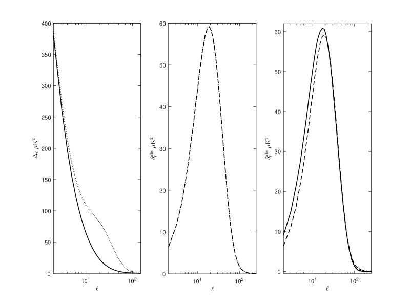
The top panels of Fig. 3 exhibit the total quantities obtained from the parameters of the first (, left) and second (, right) rows of Table 2. In these panels, solid (dotted) lines correspond to GR (AR-VTG theory with ). From the comparison of solid and dashed lines it follows that, for , there are deviations from GR in the interval represented. For , both theories lead to almost the same angular power spectrum. The relative deviations are given in the bottom panels, where it can be seen that the values of these deviations are close to (6%) for values in the interval (10,20), being greater than (1%) between and . We will not discuss the importance of these deviations, as it was already done in previous papers [6, 7] from the statistical point of view. We are only interested in the nature of these deviations, which are not either negligible or too large for the chosen value. The key question now is: what kind of effect produces the relative deviations represented in Fig. 3? To answer this question we use Figs. 4 and 5. We have to emphasize that these two figures also reveals us that, while the aforementioned relative deviations in the interval are around a 6, when the isolate contribution due LISW is consider, those deviations reach, and even exceed, a 100.
If the absolute deviations corresponding to the total quantities and those of the LISW contribution (including ) may be considered the same; namely, if the differences among these two absolute deviations are smaller than the numerical errors in the coefficients due to CAMB and VTCAMB, it can be stated that the total deviations between GR and AR-VTG are fully due to the LISW effect; however, if these differences are greater than the expected numerical errors, a part of the total deviations between GR and AR-VTG would be due to reionization through effects which are not included in the total LISW ().
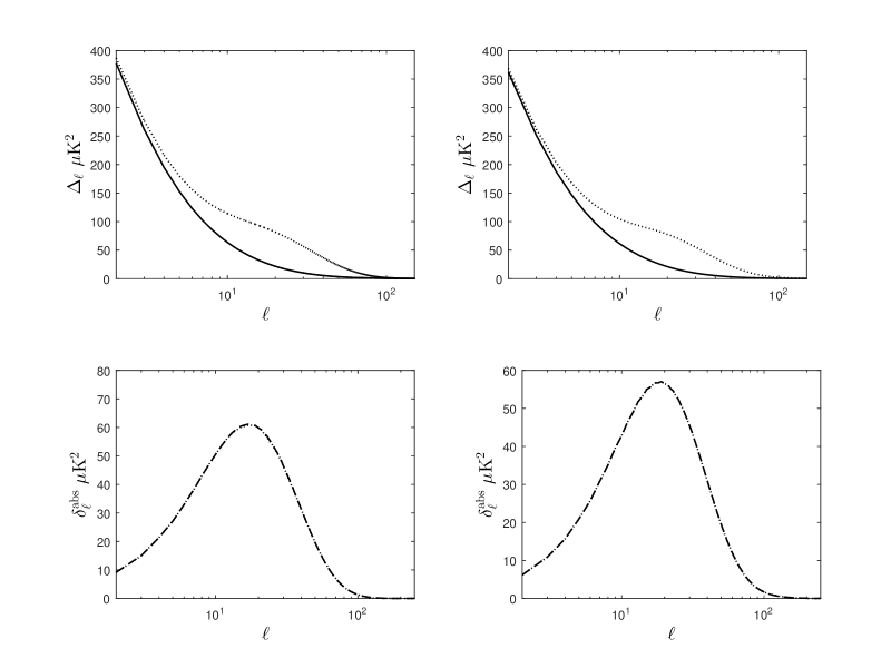
Each of the top panels of Fig. 4 has the same structure as the corresponding top panel of Fig. 3; only the displayed quantities are different in these figures: the total coefficients in Fig. 3 and the contribution due to the LISW in Fig. 4. In the bottom panels of this last Figure, there are two lines, the dashed line gives the absolute differences between GR and AR-VTG corresponding to the total coefficients represented in the top panels of Fig. 3, whereas the dotted line displays the absolute differences of the LISW contributions given in the top panels of Fig. 4. The coincidence of these lines, which are indistinguishable to the eye, suggests us that the total deviations between GR and AR-VTG are essentially due to the LISW effect (see previous paragraph). See also section 5 for a detailed measurement of the relative deviations between the dotted and dashed lines of the bottom panels.
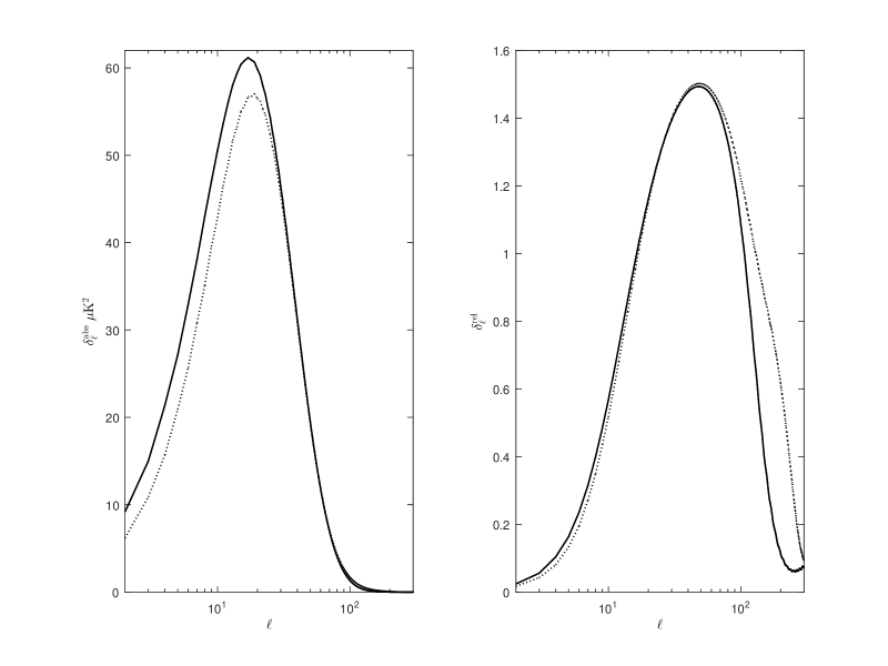
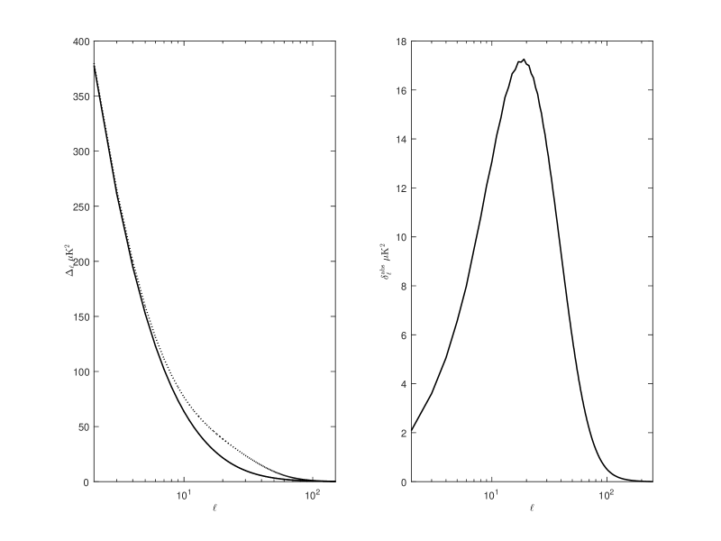
Let us now repeat our estimations of the total quantities and the LISW contributions to them in the absence of reionization. For the sake of briefness, only the results corresponding to parameters (first data row of Table 2) are presented. Similar results have been verified for parameters (second data row of Table 2). Since only the LISW effect is producing CMB anisotropy at , the total and LISW absolute deviations between GR and AR-VTG must coincide. This fact has been verified and results are presented in Fig. 5. Left and central panels of this figure have the same structure as top left and bottom left panels of Fig. 4. The two curves of the central panel are almost identical (see section 5 for measurements of deviations), which confirms that the total anisotropy is a LISW effect. Right panel shows LISW absolute deviations between GR and AR-VTG with and without reionization. It is evident that reionization affects the LISW absolute deviations (-effect), but the absolute deviations of the total quantities are affected in such a way that the two curves of the bottom left panel of Fig. 4 (with reionization) are very similar, and those of the central panel of Fig. 5 (without reionization) are also almost identical.
Fig. 6 shows absolute (left) and relative (right) differences between GR and AR-VTG for the LISW contributions to . Solid lines ( parameters) and dotted lines () do not coincide. A remarkable difference appears in both cases since reionization is very different for and parameters (see the values of parameter in Table 2). In spite of this fact, the total quantities are also different for and and, as it may be appreciate in the two bottom panels of Fig. 4, where the dotted and dashed curves almost coincide for (left) and also for (right), which strongly suggests that -whatever the fit parameters may be- total deviations are due to the LISW effect at .
3.3 The LISW in the best fit models.
Once that the nature of the deviations between RG and AR-VTG, and how these differences are generated in terms of redshift have been presented, it’s interesting to compare the LISW anisotropies predictions between best fit models.
So now, instead of use the parameter set values of a LCDM best fit model to be compared with an AR-VTG model that is built from the first one, that is, uses the mentioned parameter set values of the LCDM best fit model, plus a reasonable value for the characteristic AR-VTG parameter (D parameter), the two models to be used are: the LCDM-2013 minimal fit (see first row of Table 2) and the AR-VTG best fit model presented in Table 1.
The results of the predictions of the LISW contribution to the CMB anisotropies, of the aforementioned models, are presented in Fig. 7. As in previous comparisons, the maximum absolute differences are reached in the range of (10,20), this time those relative deviations are when examining just the LISW contributions, however, when the total CMB anisotropies are considered, those maximums are between and . It has been described in section 3.1 that a set of different results have been obtained when different evidences sources and extended models are studied (see Refs. [6, 7] for details), in this global context, we can affirm that the total CMB anisotropies differences reach a maximum between and . If we also take into account that, except in the particular case of considering tensor modes and running index, the best fit values obtained for the common parameters of GR and AR-VTG models are very similar, we may conclude that a reasonable doubt exists as to whether CMB has enough discriminating character. Another important issue to take into account is the fact that the low values of the CMB are mainly affected by cosmic variance. In such a case additional cross-correlation tests might be useful. In such a case additional cross-correlation tests might be useful.
The cross-correlation between CMB and some tracers of large scale structure surveys (LSS) was first proposed by Crittenden and Turok (see Ref. [22]), allowing us to isolate the LISW anisotropy contribution. These cross-correlations and certain statistical estimators have been successfully used to provide a physical evidence for dark energy [23], to derive constraints on the dark energy [24, 25] or neutrino masses [26], to detect coupling between dark energy and dark matter at low redshifts [27], and other issues. But also provides a mechanism for differentiating dark energy from a modified gravity, even for an identical background expansion [28, 29] which is the case we are dealing with.
Although a complete study, based on new cross-correlations, is out of the scope of current paper, we will present below some preliminary results in this regard. With this aim, next we will compare some cross-correlations theoretical predictions for GR and AR-VTG, and for that purpose, let us first introduce and define some suitable useful concepts.
The temperature fluctuation due the ISW effect in a certain direction is provided by the expression:
| (20) |
where is the visibility function of the photons, and is the gravitational potential in the Newtonian gauge. The observed density contrast for a certain direction is given by:
| (21) |
where is the galaxy bias, is the selection function of the survey, and is the matter density fluctuation. For a certain map of CMB anisotropies and a survey of galaxies the cross-correlation and the auto-correlation function are defined as:
| (22) |
and
| (23) |
with the average, denoted by the angular brackets, carried over all the pairs at the equal angular distance . For computing purposes we decompose these quantities using the Legendre polynomials :
| (24) |
the cross-correlation and the autocorrelation power spectra are obtained from:
| (25) |
and
| (26) |
respectiveliy. The function is the matter power spectrum, and the two integrals functions and are defined as follows:
| (27) |
and
| (28) |
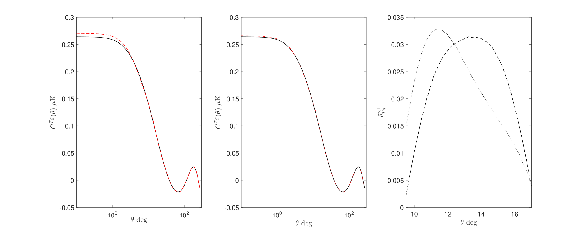
where , are the Fourier components of the gravitational potential and matter perturbations, respectively, are the spherical Bessel functions and is the commoving distance at redshift . In order to compute those related quantities a new version of the CROSS-CMBFAST [24], say VTCROSS-CMBFAST, which in turn is an adaptation of the well-known CMBFAST [30] code. In order go ahead with the calculations, some functions are still needed, these are: the galaxy bias , and the selection function of the survey . Let us consider a very simple model with and , that is we select a Gaussian distribution for selection function of the survey as in Ref. [24]. With this set of options and VTCROSS-CMBFAST, the correlation function is calculated for the models: AR-VTG best fit (see Table 1), CDM-2013 (row 1 in Table 2) and AR-VTG with (the model introduced in section 3.2).
The results are represented in Fig. 8. At this figure, one observes that both models are quite similar; there are relative differences of a located in the range , in fact the main contribution to a multipole corresponds to , so it’s something that might be expected. This is the corresponding range were we found (in the previous section) deviations between the compared models. The relative differences are defined in the same way we did in section 3.2 for .
4 On the generation of absolute deviations .
After analysing the nature of the differences between the CMB anisotropies in GR and AR-VTG, let us study how these differences are generated between redshifts 10 and 0. To do that, the differences have been estimated while the redshift varies from 10, to 5, 4, 3, 2, 1 and 0. Results are presented in Fig. 9, where each panel corresponds to one of the above redshift variations, which is given above the panel.
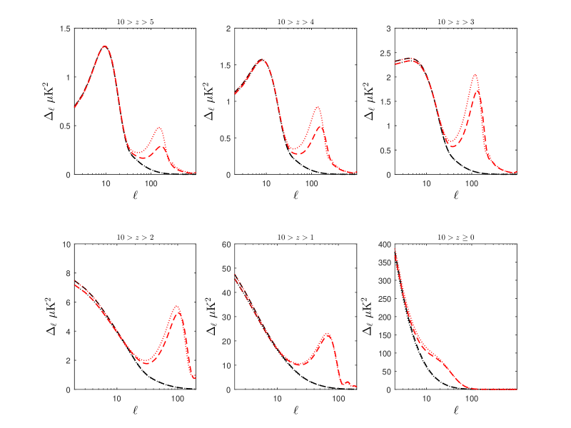
For the parameters, the black dashed lines (CDM model of GR) must be compared with the red dashed lines (AR-VTG with ). The separation between these lines measures the differences between the CMB anisotropies in GR and AR-VTG. Top left panel shows that, for , these differences reach only a few tenths of , and for (top right panel) a few ; hence, we can conclude that the differences are essentially generated for . See bottom panels for details.
The same may be concluded, for the parameters, from the comparison between black dotted lines (CDM model of GR) and red dotted lines (AR-VTG with ); hence, the conclusion that the differences between the CMB anisotropies in GR and AR-VTG is mainly generated for , is a robust conclusion almost independent on the selected parameters.
5 Discussion and conclusions.
Our main conclusions are the following: The total absolute deviations, between the CDM model of GR and AR-VTG with , are due to the LISW effect (including ). These deviations are essentially produced between redshifts 3 and 0 with the main part generated for . The relative deviations are close to 6% for and greater than 1% for .
Up to now, the nature of the aforementioned deviations has been suggested by the fact that the dotted and dashed lines of three panels are almost identical to the eye. These three panels are the left bottom panel of Fig. 4 ( parameters with reionization), the central panel of Fig. 5 ( parameters without reionization), and the right bottom panel of Fig. 4 ( parameters with reionization). Let us now prove that the relative differences, , between the dotted and the dashed lines of each of these three panels are smaller than the relative errors of CAMB and VTCAM calculations, which, based on our hard numerically computational tests and the settings we fix in terms of a balance between accuracy and performance, may be estimated to be around 1%. These relative differences are . Quantities are given in the three panels of Fig. 10. In any case, these quantities are smaller than and, consequently, they are smaller than the numerical errors.
The LISW effect, relevant for , is produced at low redshifts and, consequently, it may be detected by looking for cross correlations between the CMB temperature distribution and tracers of the dark matter distribution on large spatial scales [22]. This kind of detection has been recently achieved by using Planck data and appropriate tracers; see Ref. [31], where it is claimed that some detected cross-correlations are compatible with the CDM predictions; although other models may also be admissible. Previous detections are also listed in Ref. [31].
Since the LISW effects are distinct in the CDM model of GR and in AR-VTG with , with small relative differences (reaching values close to 6%), as it has been mentioned at the beginning of this section, the cross correlations predicted in the contexts of both models should be also different although comparable and; then, the question is: Could we select one of these models by comparing the cross-correlations predicted in them with those observed? Could we do that with high statistical significance? In section 3.1 we have outlined what could be a continuity way for this research, in such a case, we should use more complex models and estimators. A deep study on this line is out of the scope of this paper, but could lead to the selection of one of the AR-VTG models in future.

Acknowledgments
This work has been supported by the Spanish Ministry of Economía y Competitividad, MINECO-FEDER project FIS2015-64552-P and CONSOLIDER-INGENIO project CSD2010-00064. Calculations were carried out at the Centre de Càlcul de la Universitat de València. On behalf of myself and my colleague Diego (R.I.P.), I want to thank Pier-Stefano Corasaniti which has generously provide the CROSS-CMBFAST original code.
References
- [1] Planck Collaboration (P. A. R. Ade et al.), Astron. Astrophys. 594 (2016) A14.
- [2] C. M. Will, Theory and experiment in gravitational physics. (Cambridge University Press, Cambridge, 1993)
- [3] C. M. Will, Living Rev. Relativity 9 (2006) 3.
- [4] R. Dale, J.A. Morales and D. Sáez, arXiv:0906.2085 [astro-ph] (2009)
- [5] R. Dale and D. Sáez, Phys. Rev. D 85 (2012) 124047.
- [6] R. Dale and D. Sáez, Phys. Rev. D 89 (2014) 044035.
- [7] R. Dale and D. Sáez, J. Cosmol. Astropart. Phys. 01 (2017) 004.
- [8] R. Dale, M. J. Fullana and D. Sáez, Astrophys. Space Sci. 357 (2015) 116.
- [9] L. Heisenberg, J. Cosmol. Astropart. Phys. 05 (2014) 015.
- [10] J. M. Bardeen, Phys. Rev. D 22 (1980) 1882.
- [11] W. Hu and M. White, Phys. Rev. D 56 (1997) 596.
- [12] C. P. Ma, E. Bertschinger, Astrophys. J. 455 (1995) 7.
- [13] M. J. Fullana, et al., Mon. Notices Royal Astron. 464 (2017) 3784.
- [14] W. Hu and N. Sugiyama, Phys. Rev. D 50 (1994) 627.
- [15] M. Zaldarriaga and D. D. Harari, Phys. Rev. D 52 (1995) 3276.
- [16] A. Lewis, A. Challinor and A. Lasenby, Astrophys. J. 538 (2000) 473.
- [17] C. M. Will and K. Jr. Nordtvedt, Astrophys. J. 177 (1972) 757.
- [18] R. W. Hellings and K. Jr. Nordtvedt, Phys. Rev. D 7 (1973) 3593.
- [19] J. B. Jiménez and A. L. Maroto, J. Cosmol. Astropart. Phys. 03 (2009) 016.
- [20] Planck Collaboration (P. A. R. Ade et al.), Astron. Astrophys. 594 (2016) A13.
- [21] A. Lewis and S. Bridle, Phys. Rev. D 66 (2002) 103511.
- [22] R. G. Critteden and N. Turok, Phys. Rev. Lett. 76 (1996) 575.
- [23] R. Scranton et al., arXiv:astro-ph/0307335 (2003).
- [24] P. Corasaniti, T. Giannantonio, A. Melchiorri, Phys. Rev. D 71 (2005) 123521.
- [25] F. Schiavon, et al., Mon. Notices Royal Astron. 427 (2012) 3044.
- [26] J. Lesgourgues, W. Valkenburg and E. Gaztaaga, Phys. Rev. D 77 (2008) 063505.
- [27] G. Olivares, F. Atrio-Barandela and D. Pavón, Phys. Rev. D 77 (2008) 103520.
- [28] A. Lue, R. Scoccimarro and G. D. Starkman, Phys. Rev. D 69 (2004) 044005.
- [29] Y. S. Song, I. Sawicki and W. Hu, Phys. Rev. D 75 (2007) 064003.
- [30] U. Seljak and M. Zaldarriaga, Astrophys. J. 469 (1996) 437.
- [31] Planck Collaboration (P. A. R. Ade et al.), Astron. Astrophys. 571 (2014) A19.