Marrying Adapters and Mixup to Efficiently Enhance the Adversarial Robustness of Pre-Trained Language Models for Text Classification

Abstract

Existing works show that augmenting training data of neural networks using both clean and adversarial examples can enhance their generalizability under adversarial attacks. However, this training approach often leads to performance degradation on clean inputs. Additionally, it requires frequent re-training of the entire model to account for new attack types, resulting in significant and costly computations. Such limitations make adversarial training mechanisms less practical, particularly for complex Pre-trained Language Models (PLMs) with millions or even billions of parameters. To overcome these challenges while still harnessing the theoretical benefits of adversarial training, this study combines two concepts: (1) adapters, which enable parameter-efficient fine-tuning, and (2) Mixup, which train NNs via convex combinations of pairs data pairs. Intuitively, we propose to fine-tune PLMs through convex combinations of non-data pairs of fine-tuned adapters, one trained with clean and another trained with adversarial examples. Our experiments show that the proposed method achieves the best trade-off between training efficiency and predictive performance, both with and without attacks compared to other baselines on a variety of downstream tasks .

Marrying Adapters and Mixup to Efficiently Enhance the Adversarial Robustness of Pre-Trained Language Models for Text Classification

Tuc Nguyen University of Mississippi tvnguye1@go.olemiss.edu                        Thai Le University of Mississippi thaile@olemiss.edu

1 Introduction

Neural network (NN) models are susceptible to adversarial attacks that inject imperceptible noise or adversarial perturbations to the inputs to force the models to make incorrect predictions. To enhance their robustness against adversarial perturbations, several adversarial data augmentation techniques have been proposed, the most popular of which is adversarial training Goodfellow et al. (2015).

Adversarial training serves as a regularizer, enhancing a model’s accuracy by disentangling the distributions of clean and adversarial examples Miyato et al. (2018); Zhu et al. (2020). Such regularization is done by co-training NNs with both clean and perturbed examples, intuitively teaching the NNs ahead of what possible perturbations to defend against. However, training NNs that are robust against various types of adversarial perturbations in the text domain is computationally expensive. This is due to the necessity of independently re-training the models with different perturbations to accommodate different types of attack methods. This is especially important with the recent immense adoption of pre-trained language models (PLMs) in practice, most of which are very large in scale with some reaching hundreds of millions or even billions number of parameters. Moreover, adversarial training often decreases performance on clean examplesXu et al. (2021).

These observations prompt a crucial question: “Can we train PLMs on downstream tasks that can achieve better trade-off among accuracy, adversarial robustness, and computational complexity and also withstand a variety of textual attacks?” To answer this question, we seek to investigate how to incorporate adversarial training to improve NNs’ adversarial robustness without sacrificing performance on clean examples, while making minimal changes to complex PLMs during fine-tuning to minimize computational overhead.

To tackle this, this work presents a novel approach that combines two key concepts: (1) data augmentation with adversarial examples using linear interpolation, also known as Mixup Zhang et al. (2018a), and (2) efficient parameter fine-tuning for Pretrained Language Models (PLMs), often referred to as adapters Houlsby et al. (2019); Hu et al. (2022); Pfeiffer et al. (2020). Mixup technique Zhang et al. (2018a) aims to enhance both the generalizability and adversarial robustness of NNs by augmenting the models with several unique “virtual” training examples, which are obtained through convex combinations of pairs of two training data points. The use of adapters for fine-tuning PLMs is a well-established technique that requires training only on a significantly smaller number of parameters compared to the size of PLMs to adapt to downstream tasks. The innovation in this work lies in the re-purposing of Mixup to augment not between two training data points but between parameters of two adapters, one trained on clean examples and the other on adversarial examples, which are efficient by design. Our goal is to achieve more stable prediction performance on both clean and adversarial examples while minimizing the number of fine-tuning parameters.

Our contributions are summarized as follows.

1. We first motivate our work by providing a detailed analysis of the connections between data augmentation methods including adversarial training, Mixup, and model augmentation methods such as Model Soup, ensemble learning, and adapters;

2. We propose PLMs fine-tuning method AdapterMixup, which combines adversarial training, Mixup, and adapters to achieve the best trade-off between training efficiency, and predictive performance with and without attacks compared to different baselines on five standard NLP classification datasets;

3. We show that AdapterMixup also maintains a more stable performance between clean and adversarial attacks and superior efficient space and runtime complexity.

2 Related Work

2.1 Training with Data Augmentation

Let denote $f(\cdot;\theta)$ a NNs model parameterized by $\theta$, $(x_{i},y_{i})$ and $(x^{*}_{i},y^{*}_{i})$ arbitrary clean input and its adversarial example, respectively.

Adversarial Training

jointly optimizes $\theta$ on both clean and adversarial examples to improve $f$’s adversarial robustness by optimizing the loss  Goodfellow et al. (2015):

$$\alpha L(f(x;\theta),y){+}(1{-}\alpha)\max_{\delta\in S}L(f(x{+}\delta;\theta),y),$$ (1)

where $\delta$ is the adversarial perturbation, $\alpha$ controls how much the loss $L$ is updated towards the adversarial and clean version of the training input $x$ and label $y$ and $S$ is the set of allowed perturbations. When $\alpha{\leftarrow}1$, Eq. (1) converges to conventional training on only clean examples, resulting in $\theta{\leftarrow}\theta_{\operatorname{clean}}$, and when $\alpha{\leftarrow}0$, it converges to adversarial training with only adversarial examples, resulting in $\theta{\leftarrow}\theta_{\operatorname{adv}}$.

Mixup

trains a model on virtual examples constructed via linear interpolation between two random examples from the training set and their labels Zhang et al. (2018a). Mixup works out-of-the-box on continuous input modalities such as image, audio, and tabular data, and it can be applied to textual data by interpolating the word embedding vectors of input sentences (instead of their discrete tokens) Si et al. (2021). Mixup also helps to improve model robustness under a variety of mixing styles, including mixing between original examples, between original examples and their adversarial examples, and between only adversarial examples Si et al. (2021). However, Mixup shares the same inefficiency with adversarial training in practice as we need to retrain entire models every time we need to accommodate new types of attacks.

2.2 Training with Model Augmentation

Model Soup.

Model Soup improves upon ensemble learning by averaging model weights of a pool of $k$ models $\{f_{1},f_{2},\dots,f_{k}\}$ to achieve better robustness without incurring runtime required to make $k$ inference passes Wortsman et al. (2022). In principle, Model Soup is similar to Stochastic Weight Averaging (Izmailov et al., 2018) which averages model weights along an optimization trajectory. Particularly, given two model weights $\theta_{1}$ and $\theta_{2}$, Model Soup with a coefficient $\alpha{\in}[0,1]$ results in a single model with parameters:

$$\theta_{\alpha}=\alpha\theta_{1}+(1-\alpha)\theta_{2},$$ (2)

Adapter.

Adapters or parameter-efficient fine-tuning via adapters help fine-tuning PLMs on downstream tasks or with new domains efficiently Houlsby et al. (2019); Hu et al. (2022). Some works such as Pfeiffer et al. (2020) also propose to use not only one but also multiple adapters to further enhance the generalizability of the fine-tuned models.

Given $f$ with pre-trained model parameter $\theta_{0}$, fine-tuning $f$ via adapters on two domains $D_{1}$ and $D_{2}$ results in two sufficiently small adapter weights $\triangledown\theta_{1}$ and $\triangledown\theta_{2}$, respectively. This corresponds to two distinct models $f(\cdot;\theta_{0}+\triangledown\theta_{1})$ and $f(\cdot;\theta_{0}+\triangledown\theta_{2})$ during inference. Since $\triangledown\theta_{1}$ and $\triangledown\theta_{2}$ are designed to be very small in size compared to $\theta_{0}$, this approach helps achieve competitive performance compared to fully fine-tuning all model parameters $\theta_{0}$ with only a fraction of the cost.

3 Motivation

3.1 Using Mixup between Models (and not Training Examples)

Adversarial training helps enhance the adversarial robustness of NNs models. However, studies such as Xie et al. (2019) observe a consistent instability, often leading to a reduction in the trained models’ performance on clean examples. This might be a result of the substantial gap between clean and adversarial examples that can introduce non-smooth learning trajectories during training. To address this, Mixup Zhang et al. (2018b) was proposed as a data augmentation method via linear interpolation to tackle a model’s sensitivity to adversarial examples, and its instability in adversarial training. We first analyze how Mixup contributes to a more seamless learning trajectory.

Connection between Adversarial Training and Mixup. Mixup Zhang et al. (2018b) is used to regularize NNs $f$ to favor simple linear behavior in-between training examples by training $f$ on convex combinations of pairs of examples and their labels. Exploiting this property of Mixup, Si et al. (2021) proposes to adapt Mixup to augment training examples by interpolating not between only clean, but between clean and adversarial samples. Given two pairs of samples $(x_{i},y_{i})$ and its adversarial sample $(x^{*}_{i},y^{*}_{i})$, their Mixup interpolation results in:

$$(\overline{x},\overline{y}) =\operatorname{Mixup}((x_{i};y_{i}),(x^{*}_{i};y^{*}_{i}))$$ (3)

$$=[\lambda x_{i}+(1-\lambda)x^{*}_{i};\lambda y_{i}+(1-\lambda)y^{*}_{i}]$$

with $\lambda$ the interpolation coefficient. From Eq. (1), Mixup with adversarial examples under $\lambda{\leftarrow}0$ or $\lambda{\leftarrow}1$ converges to adversarial training with $\alpha{\leftarrow}0$ and $\alpha{\leftarrow}1$, respectively. Thus, to fill in the gap between clean and adversarial examples to ensure a smooth learning trajectory and overcome the instability of adversarial training, we can sample virtual training examples along with clean and adversarial examples with $\lambda{\in}(0,1)$.

Despite its benefits, Mixup necessitates re-training the whole model when facing new types of adversarial attacks, leading to additional computational costs and complicating the model debugging process. Instead of re-training, one intuitive approach is to train additional models with new adversarial knowledge and merge their weights into one single model during inference using Mixup. Thus, this motivates us to re-purpose Mixup to interpolate among models with different adversarial knowledge, instead of among training examples.

Table 1: $\theta_{i}$ represents an individual sub-model. $k$ is the total number of sub-models to be trained. $\theta_{0}$ is shared weight across all models. $\triangledown\theta_{i}$ is the adapter trained for model $i$. $\mathcal{D}_{clean}$ and $\mathcal{D}_{adv}$ refer to clean and adversarial datasets of size $N$ and $N^{\prime}$, respectively. $\mathcal{D}_{mixup}$ is the set of $kN^{\prime}$ number of interpolated examples between clean and adversarial data, generated by interpolating across $k$ instances with $N^{\prime}$ pairs of clean and adversarial examples.

	Method	Training	Space	Inference
Ensemble	$\frac{1}{k}\sum_{i=1}^{k}f\left(x\in\mathcal{D}_{clean},\theta_{i}\right)$	$\mathcal{O}(k)$	$\mathcal{O}(k)$	$\mathcal{O}(k)$
Model soup	$f\left(x\in\mathcal{D}_{clean},\frac{1}{k}\sum_{i=1}^{k}\theta_{i}\right)$	$\mathcal{O}(k)$	$\mathcal{O}(k)$	$\mathcal{O}(1)$
Mixup	$f\left(x\in\mathcal{D}_{clean}\cup\mathcal{D}_{adv}\cup\mathcal{D}_{mixup},\theta_{i}\right)$	$\mathcal{O}(1)$	$\mathcal{O}(1)$	$\mathcal{O}(1)$
AdapterMixup	$f\left(x\in\mathcal{D}_{clean}\cup\mathcal{D}_{adv},\theta_{0}+\frac{1}{k}\sum_{i=1}^{k}\triangledown\theta_{i}\right)$	$\mathcal{O}(1)$	$\mathcal{O}(1)$	$\mathcal{O}(1)$

3.2 Using Mixup on Adapters (and not Whole Models)

To simplify our analysis, we assume to use Mixup as a simple averaging function with $\lambda{=}0.5$ to merge two model parameters $\theta_{1}$ and $\theta_{2}$. In fact, merging model weights with a simple averaging function was recently proposed in Model Soup algorithm Wortsman et al. (2022). However, Model Soup’s performance is not always desirable, which we will analyze below.

Performance Analysis of Model Soup Given learned model parameters $\theta_{1}$ and $\theta_{2}$, Model Soup Wortsman et al. (2022) averages them following Eq. 2 to achieve the merged model parameters $\theta_{\alpha}$. The prediction error of the merged model $f(\cdot,\theta_{\alpha})$ over a set of $\{x,y\}_{i}$ is defined as:

$$\operatorname{Error}_{\alpha}=\mathbb{E}_{x,y}\mathbf{1}[\operatorname{argmax}_{q}f(x,\theta_{\alpha})\neq y],$$ (4)

and $\operatorname{Error}_{0}$ and $\operatorname{Error}_{1}$ are the expected errors of the model with parameter set $\theta_{1}$ and $\theta_{2}$, respectively. The ideal case happens when the expected error of the merged model $\operatorname{Error}_{\alpha}$ is lower than the best of both endpoints $\{\operatorname{Error}_{1},\operatorname{Error}_{2}\}$. However, authors of  Wortsman et al. (2022) show that this is not always the case and further compare the expected error of the merged model with the expected error of classical Ensemble Learning via merging the output logits of models with $\theta_{1}$ and $\theta_{2}$ (instead of their parameters):

$$\operatorname{Error}_{\alpha}^{enb}{=}E_{x,y}\mathbf{1}[\operatorname{argmax}_{i}f_{\alpha}^{enb}(x;\theta_{1},\theta_{2}){\neq}y],$$ (5)

where $f_{\alpha}^{\operatorname{enb}}$ is logit-ensemble of model $\theta_{1}$ and $\theta_{2}$: Wortsman et al. (2022) also shows that $\operatorname{Error}_{\alpha}^{\operatorname{enb}}$ often strictly bellow $\min\{\operatorname{Error}_{1},\operatorname{Error}_{2}\}$ for NNs $f$. Therefore, when $\operatorname{Error}_{\alpha}{\approx}\operatorname{Error}_{\alpha}^{\operatorname{enb}}$, then the $\theta_{\alpha}$ outperforms both endpoint models with $\theta_{1}$ and $\theta_{2}$. This leads us to the question of whether we can push the Model Soup’s performance closer to that of Ensemble Learning so that we only require one inference pass (in Model Soup) as compared to requiring $k$ inference passes in Ensemble Learning.

Adapters to Improve $\operatorname{Error}_{\alpha}$ Model Soup is based on a premise that, during the fine-tuning process, PLMs fine-tuned from the same pre-trained checkpoint lie in the same basin of the error landscape and close to parameter space Neyshabur et al. (2020). Consequently, averaging their model weights yields a model that can utilize a mixture of expertise without compromising the fundamental or universally acquired knowledge Wortsman et al. (2022). In contrast, when the model weights are substantially different, averaging them would result in conflicting or contradicting information acquired during pre-training, leading to poor performance. Model Soup’s authors also advocate the selection of sub-models in decreasing order of their validation accuracy on the same task for optimal results Wortsman et al. (2022), showing that the sub-models should sufficiently converge or, they are close in parameter space, especially for PLMs Neyshabur et al. (2020).

In the pursuit of a harmonized optimization trajectory, thus, we want $\theta_{1}$ and $\theta_{2}$ to exhibit substantial similarity, differing only in a few parameters responsible for their expertise. This is actually the case of Adapters, as we can decompose $\theta_{1}{=}\theta_{0}{+}\triangledown\theta_{1}$, $\theta_{2}{=}\theta_{0}{+}\triangledown\theta_{2}$ where the sizes of $\triangledown\theta_{1}$, $\triangledown\theta_{2}$ are minimal compared to $\theta_{1}$ or $\theta_{2}$ (Sec. 2.2).

Hence, this motivates us to adopt adapters to maximize the similarity in optimization trajectories between two sub-models, enabling the training of a merged model that is more competitive. Moreover, merging adapters are also more efficient, only requiring fine-tuning a small set of additional parameters $\triangledown\theta_{1}$, $\triangledown\theta_{2}$ and not the whole $\theta_{1}$ and $\theta_{2}$.

4 AdapterMixup: Mixup of Adapters with Adversarial Training

From Sec. 3, we learn that (1) Mixup on both clean and adversarial examples help stabilize adversarial training and (2) adapters allow us to efficiently achieve competitive performance of Model Soup without the need to fine-tune multiple whole pre-trained models. Thus, we propose a novel method, named AdapterMixup, that unites both Mixup and Adapters with adversarial training to efficiently enhance the robustness of PLMs. Let’s define two models with adapters at inference time: $f(\cdot;\theta_{0}{+}\triangledown\theta_{clean})$ the clean mode for prediction as we use the adapters $\triangledown\theta_{clean}$ trained on only the clean data, and $f(\cdot;\theta_{0}{+}\triangledown\theta_{\textrm{adv}})$ the adversarial mode when using the adapters $\triangledown\theta_{\textrm{adv}}$ trained on only adversarial data. Prediction after mixing the two adapters via Mixup can then be formulated as:

$$f(\cdot;\theta_{0}+[\beta\triangledown\theta_{clean}+(1-\beta)\triangledown\theta_{\textrm{adv}}]),$$ (6)

where $\beta$ is the Mixup coefficient. When $\beta{=}1$, AdapterMixup boils down to the clean mode and conversely $\beta{=}0$ corresponds to the adversarial mode.

5 Computational Complexity

Table 1 provides insights into the training, memory or space, and inference costs associated with four distinct methods, employing asymptotic notation. Overall, both Mixup and AdapterMixup exhibit optimal complexity at $\mathcal{O}(1)$ for all cost considerations. Nevertheless, during the training, the number of examples required by Mixup is greater, approximately $kN^{\prime}$, in contrast to AdapterMixup. In addition, AdapterMixup updates only a fraction of the parameter gradients, specifically $|\triangledown\theta_{i}|{<<}|\theta_{i}|$. This asymmetry in gradient updates may result in a significant reduction in the overall computational complexity, as discussed in Houlsby et al. (2019)

Attacker/Methods	MRPC		QNLI		RTE		SST2		IMDB
	Clean	Attack	Clean	Attack	Clean	Attack	Clean	Attack	Clean	Attack
TextFooler
Clean Only	90.0	50.9	94.8	56.0	85.2	33.2	95.9	42.4	92.5	51.4
Adversarial Only	68.4	68.6	49.4	66.4	52.7	74.3	51.0	59.0	52.0	69.0
Adversarial Training	87.8	64.1	92.0	64.4	84.5	59.5	95.2	56.5	90.9	76.2
ModelSoup	87.3	53.9	92.6	60.7	85.1	41.6	95.6	52.0	91.0	61.0
AdapterMixup (Ours)	88.5	64.9	94.4	67.7	81.9	48.6	96.3	56.0	92.4	66.1
PWWS
Clean Only	90.0	60.3	94.8	63.2	85.2	35.4	95.9	67.7	92.5	54.1
Adversarial Only	68.4	67.2	52.9	88.6	52.7	71.8	50.9	74.6	54.8	90.2
Adversarial Training	87.5	66.7	92.2	79.1	82.7	61.8	95.3	74.2	90.5	66.4
ModelSoup	86.0	60.8	90.9	64.7	80.2	36.9	95.9	67.7	92.7	57.6
AdapterMixup (Ours)	88.8	67.7	94.6	83.1	80.0	50.3	96.0	74.7	91.2	64.5

Table 2: Model performance of independent clean and adversarial training, traditional adversarial training with RoBERTa under TextFooler, and PWWS textual attack. In bold means better performance compared to Adversarial training. In red means performance is worse than Adversarial training.

6 Experiments

6.1 Setup

Datasets.

We assess the effectiveness of AdapterMixup on the GLUE benchmark dataset of several tasks. For a more comprehensive understanding of the benchmark datasets, detailed information is provided in Table 4 and 5 in Appendix A.1.

Robustness Evaluation

In assessing model robustness against adversarial attacks, we employ Static Attack Evaluation (SAE), a methodology that generates a predetermined set of adversarial examples on the original model acting as the victim model. Subsequently, this fixed set of adversarial examples serves as the evaluation benchmark for all the subsequent models. This evaluation setup, consistent with the approach taken in Ren et al. (2019); Tan et al. (2020); Yin et al. (2020); Wang et al. (2020); Zou et al. (2020); Wang et al. (2021), provides a standardized framework for gauging the effectiveness of models under consistent adversarial conditions.

Victim models and attack methods.

Our experimentation involves one victim model is RoBERTa-base Liu et al. (2019). As our chosen attack methods, we employ PWWS Ren et al. (2019) and TextFooler Jin et al. (2020), both known for their effectiveness in attacking state-of-the-art PLMs. Notably, both attack algorithms can access model predictions but do not utilize gradients. They iteratively explore word synonym substitutes to flip model predictions while preserving the original semantic meanings.

Baselines.

We compare AdapterMixup with several baselines as follows.

• Base Models: $\theta_{\operatorname{clean}}$, $\theta_{\operatorname{adv}}$ are two models trained with only clean examples and with only adversarial examples, respectively.

• Adversarial training  Miyato et al. (2018) where we train a single model on the augmentation of clean and adversarial data.

• Model Soup Wortsman et al. (2022) where we merging weight of two model $\theta_{clean}$ and $\theta_{adv}$.

• AdapterMixup is our method where we merge the weight of adapters which are independently learned from clean and adversarial data.

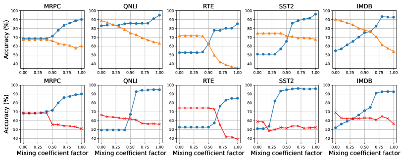
Figure 1: Performance analysis for Model Soup. The blue plots are model accuracy without attack for PWWS (above) and for TextFooler (below). The orange, red lines are prediction accuracy under attack when mixing for PWWS (above) and TextFooler (below). The horizontal axis is the mixing coefficient factor $\beta$.

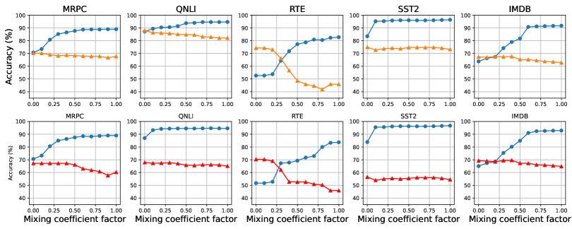
Figure 2: Performance analysis for AdapterMixup. The blue plots are model accuracy without attack for PWWS (above) and for TextFooler (below). The orange, red lines are prediction accuracy under attack when mixing for PWWS (above) and TextFooler (below). The horizontal axis is the mixing coefficient factor $\beta$.

6.2 Results

Overall.

AdapterMixup demonstrates competitive results compared to training the entire model solely on clean and adversarial examples (Table 2). Moreover, AdapterMixup approach demonstrates superior model generation and robustness compared to the Model Soup method. This observation suggests that confining the mixing to fewer parameters helps the model retain its clean performance while still achieving competitive robustness (Table 2).

In particular, under the TextFooler attack on the QNLI task, AdapterMixup achieves a performance of 94.4%, surpassing the 94.8% obtained by training the model with clean data only. Simultaneously, it maintains a performance of 67.7%, compared to 66.4% when trained exclusively on adversarial data. This illustrates that mixing a small number of model parameters not only preserves good performance on both clean and adversarial models but also generates novel hybrid representations for the shared layers, distinct from nominal and adversarial training. Similar trends are also observed in MRPC and SST2 under both TextFooler and PWWS adversarial attacks.

Generalizability and Adversarial Robustness Trade-Off.

Figure 1 shows that the accuracy and robustness landscape is depicted when using Model Soup to merge two models independently trained on clean and adversarial data. Notably, when the coefficient merging factor $\beta{\neq}1$ (clean mode), there is a significant drop in model generation, reaching its lowest point at $\beta{=}0$. In contrast, within AdapterMixup, as the coefficient factor varies in the range $[0,1]$, the changes in predictive performance between with and without attacks are more stable and minimal. Moreover, the gap between the maximum and minimum performance on robustness is considerably smaller compared to that observed in the Model Soup method (Figure 1, 2).

For a more detailed analysis of the results of the merging of entire model weights, please refer to Table 8, 9 in Appendix A.3.

Flexibility of AdapterMixup.

	MRPC	QNLI	RTE	SST2	IMDB
Clean	89.0	94.6	82.7	96.7	92.9
TextFooler	65.6	67.9	74.3	57.5	69.3
PWWS	70.2	87.9	74.3	74.9	67.3

Table 3: Model performance with independently train Adapters Houlsby et al. (2019) with RoBERTa on clean and adversarial (under TextFooler, PWWS attack) datasets.

From Table 2, it is evident that the performance of Model Soup is constrained by the limitations of its clean and adversarial versions before merging. This implies that both generalization and robustness performance consistently falls below those achieved by RoBERTa independently trained on clean and adversarial data, respectively. A similar trend is observed with AdapterMixup, where the generalization and robustness of independently trained adapters on clean and adversarial data are presented in Table 3.

However, in comparison to Model Soup, there is the option to leverage recent state-of-the-art parameter-efficient fine-tuning methods with superior performance compared to Adapters Houlsby et al. (2019), such as LoRA Hu et al. (2022) and its variants. Consequently, AdapterMixup exhibits modular properties, allowing for the defense against new types of adversarial attacks by training a new adapter corresponding to the specific text adversarial attack and subsequently merging them. Importantly, AdapterMixup supports various merging mechanisms, offering flexibility to achieve the best final model. These mechanisms may include SLERP (available at [1]), TIES-Merging Yadav et al. (2023), or DARE Yu et al. (2023).

Efficiency of AdapterMixup.

An additional advantage of mixing only clean and adversarial adapters, as opposed to the entire model weight, is the potential for saving training and inference costs through the utilization of parameter-efficient fine-tuning methods. For instance, when dealing with PLMs and various text attack methods, training a smaller set of weights on a fraction of adversarial training examples is sufficient. This was also evident in our computational complexity analysis in Sec. 5 and Table 1

7 Conclusion

In summary, this paper provides a new framework for improving model generalization and robustness of PLMs under adversarial attacks by combining adversarial training, Mixup and parameter-efficient fine-tuning via adapters. Additionally, our findings highlight the utility of adapters in empowering PLMs to achieve competitive performance in terms of generalization and robustness with and without adversarial attacks with minimal additional computational complexity.

Appendix A Appendix

A.1 Dataset statistics

Table 4 and 5 show statistics of benchmark datasets.

Dataset	MRPC	SST	QNLI
Train	3,668	67,349	104,743
Test	408	872	5,463
Dataset	RTE	IMDB
Train	2490	22,500
Test	277	2,500

Table 4: Number of instances for each dataset divided by training and test set.

Data Source	Average Document Length	Average Sentence Length	Average $\#$ Sentences per Document
MRPC	21.9	21.1	1.0
QNLI	18.2	18.0	1.0
RTE	26.2	18.1	1.4
SST	10.4	10.4	1.0
IMDB	233.8	21.6	10.8

Table 5: Length statistics.

A.2 Training details

Training details.

Tables 6, 7 show detailed hyper-parameter in our experiments.

Task	Learning rate	epoch	train batch size	evaluation batch size
BERTBASE
MRPC	2e-5	3	16	8
QNLI	3e-5	5	32	8
RTE	2e-5	3	16	8
SST2	2e-5	3	32	8
IMDB	5e-5	5	16	8
RoBERTaLARGE
MRPC	3e-5	10	32	16
QNLI	2e-4	5	32	16
RTE	3e-5	10	32	16
SST2	2e-5	5	32	16
IMDB	5e-5	5	32	16

Table 6: Hyperparameter configurations for fully finetuning on various tasks.

Task	Learning rate	epoch	batch size	warmup	weight decay	adapter size
BERTBASE
MRPC	4e-4	5	32	0.06	0.1	256
QNLI	4e-4	20	32	0.06	0.1	256
RTE	4e-4	5	32	0.06	0.1	256
SST2	4e-4	10	32	0.06	0.1	256
IMDB	4e-4	5	32	0.06	0.1	256
RoBERTaLARGE
MRPC	3e-4	5	64	0.6	0.1	64
QNLI	3e-4	20	64	0.6	0.1	64
RTE	3e-4	5	64	0.6	0.1	64
SST2	3e-4	10	64	0.6	0.1	64
IMDB	3e-4	5	64	0.6	0.1	64

Table 7: Hyperparameter configurations for adapter finetuning on various tasks.

A.3 Detailed results when mixing entire model weights

Tables 8, 9 show detailed model generation and robustness when mixing the entire model weight with coefficient $\beta$ from $0$ to $1$.

$\beta$	MRPC		QNLi		RTE		SST2		IMDB
Roberta-PWWS	Clean	Robust	Clean	Robust	Clean	Robust	Clean	Robust	Clean	Robust
0 (adv only)	68.4	67.2	82.9	88.6	52.7	71.8	50.9	74.6	54.8	90.2
0.1	68.4	67.2	83.7	86.8	52.7	71.8	50.9	74.6	56.9	88.3
0.2	68.4	67.2	83.9	84.0	52.7	71.8	50.9	74.6	61.4	86.2
0.3	68.4	67.2	83.4	82.1	52.7	71.8	50.9	74.6	65.3	84.1
0.4	68.4	67.2	85.2	78.6	53.4	71.3	56.8	74.6	70.1	80.2
0.5	71.1	66.1	85.7	74.8	62.5	62.1	65.4	71.5	75.2	78.2
0.6	77.9	63.0	85.4	72.7	77.8	49.7	85.7	70.8	76.3	76.2
0.7	83.3	61.9	85.7	69.4	77.7	42.1	88.7	69.2	82.5	70.6
0.8	86.0	60.8	85.8	66.9	80.1	39.0	90.3	69.3	93.2	61.5
0.9	88.5	57.7	90.9	64.7	80.2	36.9	91.5	69.0	92.7	57.6
1.0 (clean only)	90.0	60.3	94.8	63.2	85.2	35.4	95.9	67.7	92.5	54.1

Table 8: RoBERTa-PWWS via Model Soup

$\beta$	MRPC		QNLI		RTE		SST2		IMDB
Roberta-TextFooler	Clean	Attack	Clean	Attack	Clean	Attack	Clean	Attack	Clean	Attack
0 (adv only)	68.4	68.6	49.4	66.4	52.7	74.3	51.0	59.0	52.0	69.0
0.1	68.4	68.6	49.5	64.4	52.7	74.3	51.0	58.5	56.2	63.0
0.2	68.4	68.6	49.5	64.0	52.7	74.3	53.7	48.5	59.3	62.1
0.3	68.9	68.6	49.5	63.1	52.7	74.3	82.2	50.0	62.1	62.5
0.4	70.3	68.6	49.5	62.4	52.7	74.3	93.3	52.3	66.4	62.5
0.5	71.6	55.5	67.1	62.0	52.7	74.3	94.8	51.5	71.3	63.1
0.6	80.1	55.5	92.6	60.7	57.4	73.0	95.7	54.0	75.0	62.8
0.7	86.0	54.2	94.2	56.9	76.5	55.1	96.2	54.0	91.0	61.0
0.8	87.3	53.9	94.5	56.3	83.0	41.9	95.6	51.5	92.5	64.8
0.9	89.2	53.0	94.9	56.5	85.1	41.6	95.6	52.0	92.7	62.8
1.0 (clean only)	90.0	50.9	94.8	56.0	85.2	39.2	95.9	52.4	92.5	56.4

Table 9: RoBERTa-TextFooler via Model Soup

References

- Goodfellow et al. (2015) Ian J Goodfellow, Jonathon Shlens, and Christian Szegedy. 2015. Explaining and harnessing adversarial examples. ICLR.
- Houlsby et al. (2019) Neil Houlsby, Andrei Giurgiu, Stanislaw Jastrzebski, Bruna Morrone, Quentin De Laroussilhe, Andrea Gesmundo, Mona Attariyan, and Sylvain Gelly. 2019. Parameter-efficient transfer learning for nlp. In ICML, pages 2790–2799. PMLR.
- Hu et al. (2022) Edward J Hu, Yelong Shen, Phillip Wallis, Zeyuan Allen-Zhu, Yuanzhi Li, Shean Wang, Lu Wang, and Weizhu Chen. 2022. Lora: Low-rank adaptation of large language models. In ICLR.
- Izmailov et al. (2018) Pavel Izmailov, Dmitrii Podoprikhin, Timur Garipov, Dmitry Vetrov, and Andrew Gordon Wilson. 2018. Averaging Weights Leads to Wider Optima and Better Generalization. Uncertainty in Artificial Intelligence.
- Jin et al. (2020) Di Jin, Zhijing Jin, Joey Tianyi Zhou, and Peter Szolovits. 2020. Is BERT really robust? A strong baseline for natural language attack on text classification and entailment. In Proceedings of AAAI 2020.
- Liu et al. (2019) Yinhan Liu, Myle Ott, Naman Goyal, Jingfei Du, Mandar Joshi, Danqi Chen, Omer Levy, Mike Lewis, Luke Zettlemoyer, and Veselin Stoyanov. 2019. RoBERTa: A Robustly Optimized BERT Pretraining approach. arXiv.
- Miyato et al. (2018) Takeru Miyato, Shin-ichi Maeda, Masanori Koyama, and Shin Ishii. 2018. Virtual adversarial training: a regularization method for supervised and semi-supervised learning. IEEE transactions on pattern analysis and machine intelligence.
- Neyshabur et al. (2020) Behnam Neyshabur, Hanie Sedghi, and Chiyuan Zhang. 2020. What is being transferred in transfer learning? NeurIPS.
- Pfeiffer et al. (2020) Jonas Pfeiffer, Aishwarya Kamath, Andreas Rücklé, Kyunghyun Cho, and Iryna Gurevych. 2020. Adapterfusion: Non-destructive task composition for transfer learning. arXiv preprint arXiv:2005.00247.
- Ren et al. (2019) Shuhuai Ren, Yihe Deng, Kun He, and Wanxiang Che. 2019. Generating Natural Language Adversarial Examples through Probability Weighted Word Saliency. In Proceedings of ACL 2019.
- Si et al. (2021) Chenglei Si, Zhengyan Zhang, Fanchao Qi, Zhiyuan Liu, Yasheng Wang, Qun Liu, and Maosong Sun. 2021. Better robustness by more coverage: Adversarial and mixup data augmentation for robust finetuning. In Findings of the Association for Computational Linguistics: ACL-IJCNLP.
- Tan et al. (2020) Samson Tan, Shafiq Joty, Min-Yen Kan, and Richard Socher. 2020. It’s morphin’ time! Combating linguistic discrimination with inflectional perturbations. In Proceedings of ACL 2020.
- Wang et al. (2021) Boxin Wang, Shuohang Wang, Y. Cheng, Zhe Gan, Ruoxi Jia, Bo Li, and Jingjing Liu. 2021. InfoBERT: Improving Robustness of Language Models from An Information Theoretic Perspective. In Proceedings of ICLR 2021.
- Wang et al. (2020) Tianlu Wang, Xuezhi Wang, Yao Qin, Ben Packer, Kang Li, Jilin Chen, Alex Beutel, and Ed Chi. 2020. CAT-gen: Improving robustness in NLP models via controlled adversarial text generation. In Proceedings of EMNLP 2020.
- Wortsman et al. (2022) Mitchell Wortsman, Gabriel Ilharco, Samir Ya Gadre, Rebecca Roelofs, Raphael Gontijo-Lopes, Ari S Morcos, Hongseok Namkoong, Ali Farhadi, Yair Carmon, Simon Kornblith, et al. 2022. Model soups: averaging weights of multiple fine-tuned models improves accuracy without increasing inference time. In ICML. PMLR.
- Xie et al. (2019) Cihang Xie, Mingxing Tan, Boqing Gong, Jiang Wang, Alan Yuille, and Quoc V Le. 2019. Adversarial Examples Improve Image Recognition. arXiv preprint arXiv:1911.09665.
- Xu et al. (2021) Han Xu, Xiaorui Liu, Yaxin Li, Anil Jain, and Jiliang Tang. 2021. To be robust or to be fair: Towards fairness in adversarial training. In International conference on machine learning, pages 11492–11501. PMLR.
- Yadav et al. (2023) Prateek Yadav, Derek Tam, Leshem Choshen, Colin Raffel, and Mohit Bansal. 2023. Ties-merging: Resolving interference when merging models. In Thirty-seventh Conference on Neural Information Processing Systems.
- Yin et al. (2020) Fan Yin, Quanyu Long, Tao Meng, and Kai-Wei Chang. 2020. On the Robustness of Language Encoders against Grammatical Errors. In Proceedings of ACL 2020.
- Yu et al. (2023) Le Yu, Bowen Yu, Haiyang Yu, Fei Huang, and Yongbin Li. 2023. Language models are super mario: Absorbing abilities from homologous models as a free lunch. arXiv preprint arXiv:2311.03099.
- Zhang et al. (2018a) Hongyi Zhang, Moustapha Cisse, Yann N Dauphin, and David Lopez-Paz. 2018a. mixup: Beyond empirical risk minimization. ICLR.
- Zhang et al. (2018b) Hongyi Zhang, Moustapha Cissé, Yann N. Dauphin, and David Lopez-Paz. 2018b. mixup: Beyond empirical risk minimization. In Processings of ICLR 2018.
- Zhu et al. (2020) Chen Zhu, Yu Cheng, Zhe Gan, Siqi Sun, Tom Goldstein, and Jingjing Liu. 2020. Freelb: Enhanced adversarial training for natural language understanding. ICLR.
- Zou et al. (2020) Wei Zou, Shujian Huang, John Xie, Xin-Yu Dai, and Jiajun Chen. 2020. A Reinforced Generation of Adversarial Samples for Neural Machine Translation. In Proceedings of ACL 2020.