Level spacing distribution of localized phases induced by quasiperiodic potentials
Abstract
Level statistics is a crucial tool in the exploration of localization physics. The level spacing distribution of the disordered localized phase follows Poisson statistics, and many studies naturally apply it to the quasiperiodic localized phase. Here we analytically obtain the level spacing distribution of the quasiperiodic localized phase, and find that it deviates from Poisson statistics. Moreover, based on this level statistics, we derive the ratio of adjacent gaps and find that for a single sample, it is a function, which is in excellent agreement with numerical studies. Additionally, unlike disordered systems, in quasiperiodic systems, there are variations in the level spacing distribution across different regions of the spectrum, and increasing the size and increasing the sample are non-equivalent. Our findings carry significant implications for the reevaluation of level statistics in quasiperiodic systems and a profound understanding of the distinct effects of quasiperiodic potentials and disorder induced localization.
Introduction.— Quantum localization has consistently been a significant research area in condensed matter physics. This phenomenon is widely present in disordered systems, caused by interference from multiply scattered waves due to system disorder, resulting in the exponential decay of the wave function and the suppression of transport Anderson1958 ; RMP1 ; RMP2 ; Kramer1993 . In addition to random disorder, quasiperiodic potentials also induce localization, and in recent years, they have garnered widespread interest in both theoretical Soukoulis1981 ; DasSarma1988 ; Biddle2009 ; XLi2017 ; HYao2019 ; Ganeshan2015 ; Wang1 ; XCZhou ; Wang2022 ; XDeng2019 ; Ribeiro and experimental Roati2008 ; Bloch4 ; An2018 ; JiasT ; TXiao2021 ; Weld ; HengFan aspects, playing a crucial role in enhancing our understanding of critical phases TXiao2021 ; Weld ; HengFan ; WangYC2021 ; Kohmoto1990 , rich transport behaviors LandiRMP ; Saha ; Dwiputra ; Lacerda ; Jeffrey , many-body localization (MBL) IBlochRMP ; BAA ; Schreiber2015 , low dimensional Anderson transition and mobility edges Soukoulis1981 ; DasSarma1988 ; Biddle2009 ; XLi2017 ; HYao2019 ; Ganeshan2015 ; Wang1 ; XCZhou ; Wang2022 ; XDeng2019 ; Ribeiro ; Roati2008 ; Bloch4 ; An2018 ; JiasT .
The energy level distribution of localized phases is completely distinct from that of extended phases, allowing us to use level spacing statistics to differentiate between extended and localized phases Shklovskii1993 ; Mirlin2000 . For disordered systems, the energy levels of the localized phase are uncorrelated, with no level repulsion, and their distribution follows Poisson statistics Shklovskii1993 ; Mirlin2000 ; Molcanov1981 . Extending the statistical patterns of energy levels for disorder-induced localized phases to quasiperiodic-induced localized phases seems natural. Additionally, the average of the adjacent gap ratio is close to 0.387 XLi2016 ; YLiu2020 ; YWang2023 ; Xianlong ; Ray2016 ; JHPixley ; Schiffer2021 ; Ray2018 ; Khemani2017 ; Roushan2017 ; XiaopengLi ; Modak2015 , which is in complete agreement with the results predicted by Poisson statistics. Therefore, the level statistics of quasiperiodic localization systems are widely accepted to follow Poisson statistics in both single-particle XLi2016 ; YLiu2020 ; YWang2023 ; Xianlong ; Ray2016 ; JHPixley ; Schiffer2021 ; Ray2018 ; Machida1986 ; SNEvangelou ; Roy2019 ; Takada2004 ; YWang2016 and many-body systems Khemani2017 ; Roushan2017 ; XiaopengLi ; Modak2015 . However, recent mathematical proof has shown that the distribution of eigenvalues in quasiperiodic and disordered localized phases exhibits significant differences Jitomirskaya , implying that the patterns of energy level spacings for the two cases may also differ. This inspires us to reexamine the level spacing distribution of the quasiperiodic localized phase and the spectrum’s differences between this and localized phase induced by disorder.
In this letter, we investigate the level spacing distribution of localized phases induced by quasiperiodic potentials. We first compare the energy level distribution , level spacing distribution and the distribution of the adjacent gap ratio for Anderson localization (AL) phase induced by quasi-periodic potentials with those induced by disorder. Next, we calculate the number variance of different regions of energy spectrum in the Aubry-André (AA) model AA . Then, we analytically derive and for the AA model’s AL phase. Finally, we calculate and discuss the probability distribution when interactions are present.
Model and results.— The AA model is the simplest nontrivial example with a one-dimensional quasiperiodic potential, described by
| (1) |
where () denotes the annihilation (creation) operator at site , is the nearest-neighbor hopping coefficient, and with , and being the quasiperiodic potential amplitude, the phase offset, and an irrational number, respectively. This model demonstrates self-duality in the transformation between lattice space and its dual space at , resulting in the Anderson transition with all eigenstates being extended (localized) for () AA . For simplicity, we fix and set with being the Fibonacci sequence (i.e., , , and ). As approaches infinity, converges to . Unless otherwise stated, we take the system size , and use open boundary conditions.
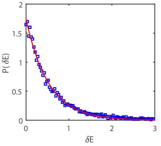
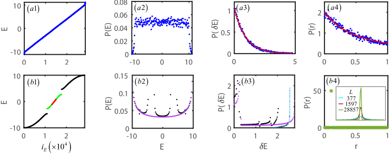
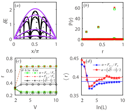
We first compare the level spacing distributions of the localized phase in the AA model with that induced by random disorder, as shown in Fig. 1. For the disorder-induced localization, we consider the above Eq. (1), with the onsite disorder being uniformly distributed in the interval . We observe that the energy spectrum of localized phases caused by disorder does not exhibit significant large gaps [Fig. 1(a1)]. Apart from a decrease in the density of states (DOS) at the boundaries of the spectrum, the DOS across the spectrum is uniformly distributed [Fig. 1(a2)]. As a contrast, the energy spectrum of quasiperiodic localized phases shows two distinct large gaps, dividing the spectrum into three segments [Fig. 1(b1)]. The numbers of states in each segment from bottom to top are , , , and at the boundaries of each segment, the DOS increases [Fig. 1(b2)]. Then we compare the distribution of energy level spacings, defined as , with the eigenvalues listed in ascending order. In the disorder system, the level statistics of localized phases are Poisson: [Fig. 1(a3)], where and is the average of . Based on the energy level spacing, we can obtain the ratio of adjacent gaps as DAHuse1 ; DAHuse2 . For Poisson statistics, one can derive that the distribution of satisfies [Fig. 1(a4)], which gives the average value of as . However, for the quasiperiodic localized phase, the energy level spacing noticeably deviates from Poisson statistics, as indicated by the black data points in Fig. 1(b3). The distribution is not but rather takes on the form of a function [Fig. 1(b4)].
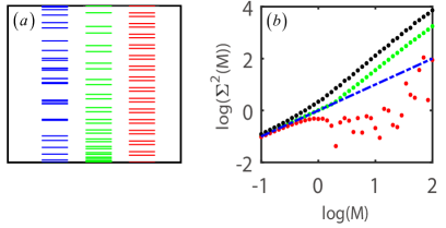
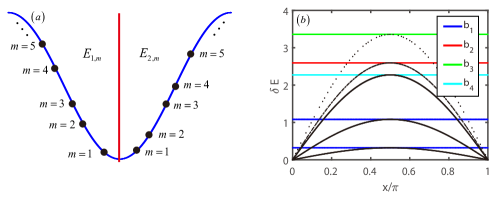
Before deriving the distributions and , we first investigate the uniformity of level spacings across different regions in the spectrum. Fig. 2(a) displays three types of spectra, corresponding to the localized phase in disordered systems and the edge and middle regions in the middle segment of Fig. 1(b1). The distances between the energy levels of the disordered system (blue lines) show significant fluctuations and lack correlation, allowing levels to approach each other arbitrarily closely. Similar properties are observed in the boundaries of the quasi-periodic system’s energy spectrum (green lines). However, in the middle region of each segment of the energy spectrum, level repulsion is observed, expressing the unlikelihood of levels being degenerate in this system. This suggests that the energy spectrum of the localized phase in quasi-periodic systems does not lack correlation between energy levels as observed in disordered systems. To characterize the uniformity of energy level spacings, we investigate the level number variance , defined as , where quantifies the number of levels within the width on the unfolded scale Dyson1963 ; Guhr1998 ; Bertrand2016 ; WangMBC . For Poisson statistics, the spectrum exhibits no correlations, resulting in a number variance that is exactly linear with a slope of one, i.e., (blue dashed line in Fig. 2(b)). Fig. 2(a) shows that the distribution of energy levels in the middle region of each segment of the energy spectrum is more uniform, leading to a smaller (red dots in Fig. 2(b)), similar to that is obtained from the Wigner-Dyson distribution. For each segment’s boundary region (green dots in Fig. 2(b)) and the overall energy spectrum (black dots in Fig. 2(b)), when is large, the linear slope of their respective is greater than . This indicates that their energy level distribution is more uneven than the Poisson distribution. To the best of our knowledge, the spectra that satisfy the condition of the number variance being linear with a slope greater than have not been reported before.
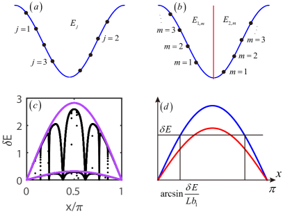
We now deduce the level spacing distribution in the AL phase of the AA model. We set , , and fix , then the system’s eigenvalues are , with [Fig. 3(a)]. We introduce , setting it equal to mod(), then , and it is easy to verify that the range of is . Shifting the labels of energies with , one can obtain
| (2) |
By selecting the appropriate value for , one can make the range of satisfy explain1 . We then separate the energy levels into two parts, as shown in Fig. 3(b). For we denote the energies by ; for we relabel and denote the energies by , hence and , with . It is convenient to introduce variables and , and then the energies become
| (3) |
The energies are naturally ordered:
| (4) |
If , the total energies are ordered by , thus and . Combining Eq. (3), we can obtain that
| (5) |
where and . When , , one can obtain Eq. (5), and it still holds true, with the only difference being that and .
We consider the limit and hence . For the sake of convenience and comparison, we consider , and combining Eq. (5), we obtain
| (6) |
Similarly,
| (7) |
We note that and are of the order of , so and are of the order of . Therefore, the distribution of consists of two branches, as shown in Fig. 3(c), and these two branches satisfy Eq. (6) and Eq. (7), respectively. Then one can calculate that the total number of states for the energy smaller than is [see Fig. 3(d)]. Hence the probability distribution is
| (8) |
Similarly, one can obtain . The total probability distribution should be considered as the sum of the two.
We previously discussed the case of . For the general case, it is challenging to derive its expression. However, considering the statistically unified form for the level spacing distribution induced by disorder, with the fitting parameters and changing with increasing disorder strength, we believe that for AL induced by quasi-periodic potential, the level spacing distribution should satisfy a unified form
| (9) |
where is the step function explaintheta , represents the number of branches, and are the undetermined parameters that describe the scaling and translation of with . In Fig. 1(b3), the purple and light blue dashed lines correspond to the fitting results using Eq. (8) (corresponding to ) and Eq. (9), respectively. We observe that Eq. (9) can effectively describe the level spacing distribution of quasiperiodic AL.
We further derive the distribution of the adjacent gap ratio through the use of the defining equation . For the case of , and respectively correspond to the two purple lines in Fig. 3(c), which are described by Eq. (6) and Eq. (7). Considering , can be brought outside the integral, so
| (10) |
Thus, the distribution is function, as shown in Fig. 1(b4), which is clearly different from the given by Poisson statistics. When , the number of branches of (i.e., in Eq. (9)) will exceed (see Supplementary Material SM ), as shown in Fig. 4(a). Consequently, multiple peaks appear in , as depicted in Fig. 4(b). For the case of , using perturbation theory, we can demonstrate that and in Eq. (5) need to be multiplied by the same factor SM . Therefore, from Eq. (10), is independent of both and in the AL phase. Additionally, the expressions for and include the initial phase , hence the peak positions of depend on . From Fig. 4(c), we observe that the values of are independent of and the position in the energy spectrum. However, they depend on and on whether takes the value or .
Then we consider the sample average of , which is equivalent to average over , i.e., with and or and . Substituting the expressions for and , one easily obtains SM , as shown in Fig. 4(d). We note that although the result of is the same as that given by Poisson distribution, it is not caused by Poisson statistics. When , is a value close to , distinct from [Fig. 4(d)]. When the interaction is added, even with a fixed , the level spacing distribution of the quasiperiodic MBL phase still follows Poisson statistics SM .
Conclusion and Discussion.— We have derived the level-spacing distribution of quasiperiodic AL phase, which satisfies Eq. (9) and found that it does not follow Poisson statistics, whereas quasiperiodic MBL’s spectrum conforms to Poisson statistics. In addition, we found more differences in the spectrum between the quasiperiodic and disordered AL phases. Specifically: (1) the former exhibits different degrees of uniformity in level spacing across different spectral regions, and the overall distribution is even more uneven than a Poisson distribution, whereas the latter shows a relatively uniform level distribution across different spectral regions; (2) the distribution of for the former is a function dependent only on the initial phase, while the distribution of for the latter follows ; (3) the sample-averaged value for the former depends on whether or . Although, for the case of , the obtained is the same as that obtained from Poisson statistics, it does not originate from Poisson statistics. Further, there are spatial correlations in quasiperiodic systems, indicating that increasing the number of samples is not equivalent to increasing the size, which is in contrast to Poisson statistics. The energy spectrum of quasiperiodic systems can be experimentally determined in various systems, such as semiconductor quantum dots Kiczynski2022 or superconducting qubits Roushan2017 .
Acknowledgements.
We thank Qi Zhou for making us aware of Ref. Jitomirskaya . This work is supported by National Key R&D Program of China under Grant No.2022YFA1405800, the National Natural Science Foundation of China (Grant No.12104205), the Key-Area Research and Development Program of Guangdong Province (Grant No. 2018B030326001), Guangdong Provincial Key Laboratory (Grant No.2019B121203002).References
- (1) P. W. Anderson, Phys. Rev. 109, 1492 (1958).
- (2) P. A. Lee and T. V. Ramakrishnan, Disordered electronic systems, Rev. Mod. Phys. 57, 287 (1985).
- (3) F. Evers and A. D. Mirlin, Anderson transitions, Rev. Mod. Phys. 80, 1355 (2008).
- (4) B. Kramer and A. MacKinnon, Localization: theory and experiment, Rep. Prog. Phys. 56, 1469 (1993).
- (5) C. M. Soukoulis and E. N. Economou, Localization in One-Dimensional Lattices in the Presence of Incommensurate Potentials, Phys. Rev. Lett. 48, 1043 (1981).
- (6) S. Das Sarma, S. He, and X. C. Xie, Mobility edge in a model one-dimensional potential, Phys. Rev. Lett. 61, 2144 (1988).
- (7) J. Biddle, B. Wang, D. J. Priour Jr, and S. Das Sarma, Localization in one-dimensional incommensurate lattices beyond the Aubry-André model, Phys. Rev. A 80, 021603 (2009); J. Biddle and S. Das Sarma, Predicted mobility edges in one-dimensional incommensurate optical lattices: an exactly solvable model of Anderson localization, Phys. Rev. Lett. 104, 070601 (2010).
- (8) X. Li, X. Li, and S. Das Sarma, Mobility edges in one dimensional bichromatic incommensurate potentials, Phys. Rev. B 96, 085119 (2017); D. Vu and S. Das Sarma, Generic mobility edges in several classes of duality-breaking one-dimensional quasiperiodic potentials, Phys. Rev. B 107, 224206 (2023).
- (9) H. Yao, H. Khoudli, L. Bresque, and L. Sanchez-Palencia, Critical behavior and fractality in shallow one-dimensional quasiperiodic potentials, Phys. Rev. Lett. 123, 070405 (2019).
- (10) S. Ganeshan, J. H. Pixley, and S. Das Sarma, Nearest neighbor tight binding models with an exact mobility edge in one dimension, Phys. Rev. Lett. 114, 146601 (2015).
- (11) Y. Wang, X. Xia, L. Zhang, H. Yao, S. Chen, J. You, Q. Zhou, and X.-J. Liu, One dimensional quasiperiodic mosaic lattice with exact mobility edges, Phys. Rev. Lett. 125, 196604 (2020).
- (12) X.-C. Zhou, Y. Wang, T.-F. J. Poon, Q. Zhou, and X.-J. Liu, Exact new mobility edges between critical and localized states, Phys. Rev. Lett. 131, 176401 (2023).
- (13) Y. Wang, L. Zhang, W. Sun, T.-F. J. Poon, and X.-J. Liu, Quantum phase with coexisting localized, extended, and critical zones, Phys. Rev. B 106, L140203 (2022).
- (14) X. Deng, S. Ray, S. Sinha, G. Shlyapnikov, and L. Santos, One-dimensional quasicrystals with power-law hopping, Phys. Rev. Lett. 123, 025301 (2019).
- (15) M. Gonçalves, B. Amorim, E. V. Castro, and P. Ribeiro, Hidden dualities in 1D quasiperiodic lattice models, SciPost Phys. 13, 046 (2022); M. Gonçalves, B. Amorim, E. V. Castro, and P. Ribeiro, Renormalization-Group Theory of 1D quasiperiodic lattice models with commensurate approximants, Phys. Rev. B 108, L100201 (2023); M. Gonçalves, B. Amorim, E. V. Castro, and P. Ribeiro, Critical phase dualities in 1D exactly-solvable quasiperiodic models, Phys. Rev. Lett. 131, 186303 (2023).
- (16) G. Roati, C. D’Errico, L. Fallani, M. Fattori, C. Fort, M. Zaccanti, G. Modugno, M. Modugno, and M. Inguscio, Anderson localization of a non-interacting Bose-Einstein condensate, Nature (London) 453, 895 (2008).
- (17) H. P. Lüschen, S. Scherg, T. Kohlert, M. Schreiber, P. Bordia, X. Li, S. D. Sarma, and I. Bloch, Single-particle mobility edge in a one-dimensional quasiperiodic optical lattice, Phys. Rev. Lett. 120, 160404 (2018);T. Kohlert, S. Scherg, X. Li, H. P. Lüschen, S. D. Sarma, I. Bloch, and M. Aidelsburger, Observation of many-body localization in a one-dimensional system with single-particle mobility edge, Phys. Rev. Lett. 122, 170403 (2019).
- (18) F. A. An, E. J. Meier, and B. Gadway, Engineering a flux-dependent mobility edge in disordered zigzag chains, Phys. Rev. X 8, 031045 (2018); F. A. An, K. Padavić, E. J. Meier, S. Hegde, S. Ganeshan, J. H. Pixley, S. Vishveshwara, and B. Gadway, Observation of tunable mobility edges in generalized Aubry-André lattices, Phys. Rev. Lett. 126, 040603 (2021).
- (19) Y. Wang, J.-H. Zhang, Y. Li, J. Wu, W. Liu, F. Mei, Y. Hu, L. Xiao, J. Ma, C. Chin, and S. Jia, Observation of Interaction-Induced Mobility Edge in an Atomic Aubry-André Wire, Phys. Rev. Lett. 129, 103401 (2022).
- (20) T. Xiao, D. Xie, Z. Dong, T. Chen, W. Yi, and B. Yan, Observation of topological phase with critical localization in a quasi-periodic lattice, Science Bulletin 66, 2175 (2021).
- (21) T. Shimasaki, M. Prichard, H. E. Kondakci, J. Pagett, Y. Bai, P. Dotti, A. Cao, T.-C. Lu, T. Grover, and D. M. Weld, Anomalous localization and multifractality in a kicked quasicrystal, arXiv:2203.09442.
- (22) H. Li, Y.-Y. Wang, Y.-H. Shi, K. Huang, X. Song, G.-H. Liang, Z.-Y. Mei, B. Zhou, H. Zhang, J.-C. Zhang, et al., Observation of critical phase transition in a generalized Aubry-André-Harper model with superconducting circuits, npj Quantum Information 9, 40 (2023).
- (23) Y. Wang, L. Zhang, S. Niu, D. Yu, X.-J. Liu, Realization and detection of non-ergodic critical phases in optical Raman lattice, Phys. Rev. Lett. 125, 073204 (2020).
- (24) Y. Hatsugai and M. Kohmoto, Energy spectrum and the quantum Hall effect on the square lattice with next-nearest-neighbor hopping, Phys. Rev. B 42, 8282 (1990); J. H. Han, D. J. Thouless, H. Hiramoto, and M. Kohmoto, Critical and bicritical properties of Harper’s equation with next-nearest-neighbor coupling, Phys. Rev. B 50, 11365 (1994).
- (25) G. T. Landi, D. Poletti, and G. Schaller, Nonequilibrium boundary-driven quantum systems: Models, methods, and properties, Rev. Mod. Phys. 94, 045006 (2022).
- (26) M. Saha, S. K. Maiti, and A. Purkayastha, Anomalous transport through algebraically localized states in one dimension, Phys. Rev. B 100, 174201 (2019); A. Purkayastha, A. Dhar, and M. Kulkarni, Nonequilibrium phase diagram of a one-dimensional quasiperiodic system with a single-particle mobility edge, Nonequilibrium phase diagram of a one-dimensional quasiperiodic system with a single-particle mobility edge, Phys. Rev. B 96, 180204(R) (2017); M. Saha, B. P. Venkatesh, and B. K. Agarwalla, Quantum transport in quasiperiodic lattice systems in the presence of Büttiker probes, Phys. Rev. B 105, 224204 (2022).
- (27) D. Dwiputra and F. P. Zen, Environment-assisted quantum transport and mobility edges, Phys. Rev. A 104, 022205 (2021).
- (28) A. M. Lacerda, J. Goold, and G. T. Landi, Dephasing enhanced transport in boundary-driven quasiperiodic chains, Phys. Rev. B 104, 174203 (2021); V. Balachandran, S. R. Clark, J. Goold, and D. Poletti, Energy Current Rectification and Mobility Edges, Phys. Rev. Lett. 123, 020603 (2019); C. Chiaracane, M. T. Mitchison, A. Purkayastha, G. Haack, and J. Goold, Quasiperiodic quantum heat engines with a mobility edge, Phys. Rev. Research 2, 013093 (2020).
- (29) T.-F. J. Poon, Y. Wan, Y. Wang, and X.-J. Liu, Anomalous quantum transport in 2D asymptotic quasiperiodic system, arXiv:2312.04349.
- (30) D. A. Abanin, E. Altman, I. Bloch, and M. Serbyn, Colloquium: Many-body localization, thermalization, and entanglement, Rev. Mod. Phys. 91, 021001 (2019).
- (31) D. M. Basko, I. L. Aleiner, and B. L. Altshuler, Metal-insulator transition in a weakly interacting many-electron system with localized single-particle states, Ann. Phys. 321, 1126 (2006).
- (32) M. Schreiber, S. S. Hodgman, P. Bordia, H. P. Lüschen, M. H. Fischer, R. Vosk, E. Altman, U. Schneider, and I. Bloch, Observation of many-body localization of interacting fermions in a quasirandom optical lattice, Science 349, 842 (2015).
- (33) B. I. Shklovskii, B. Shapiro, B. R. Sears, P. Lambrianides, and H. B. Shore, Statistics of spectra of disordered systems near the metal-insulator transition, Phys. Rev. B 47, 11487 (1993).
- (34) A. D. Mirlin, Statistics of energy levels and eigenfunctions in disordered systems, Phys. Rep. 326, 259 (2000).
- (35) S. A. Molčanov, The Local Structure of the Spectrum of the One-Dimensional Schrödinger Operator, Commun. Math. Phys. 78, 429 (1981).
- (36) X. Li, J. H. Pixley, D.-L. Deng, S. Ganeshan, and S. Das Sarma, Quantum nonergodicity and fermion localization in a system with a single-particle mobility edge, Phys. Rev. B 93, 184204 (2016).
- (37) Y. Liu, X.-P. Jiang, J. Cao, and S. Chen, Non-Hermitian mobility edges in one-dimensional quasicrystals with parity-time symmetry, Phys. Rev. B 101, 174205 (2020).
- (38) Y. Wang, L. Zhang, Y. Wan, Y. He, and Y. Wang, Two-dimensional vertex-decorated Lieb lattice with exact mobility edges and robust flat bands, Phys. Rev. B 107, L140201 (2023).
- (39) S. Cheng, R. Asgari, and G. Xianlong, From topological phase to transverse Anderson localization in a two-dimensional quasiperiodic system, Phys. Rev. B 108, 024204 (2023).
- (40) S. Ray, M. Pandey, A. Ghosh and S. Sinha, Localization of weakly interacting Bose gas in quasiperiodic potential, New J. Phys. 18, 013013 (2016).
- (41) J. H. Pixley, J. H. Wilson, D. A. Huse, and S. Gopalakrishnan, Weyl Semimetal to Metal Phase Transitions Driven by Quasiperiodic Potentials, Phys. Rev. Lett. 120, 207604 (2018).
- (42) S. Schiffer, X.-J. Liu, H. Hu, and J. Wang, Anderson localization transition in a robust PT-symmetric phase of a generalized Aubry-André model, Phys. Rev. A 103, L011302 (2021).
- (43) S. Ray, A. Ghosh, and S. Sinha, Drive-induced delocalization in the Aubry-André model, Phys. Rev. E 97, 010101(R) (2018).
- (44) V. Khemani, D. N. Sheng, and D. A. Huse, Two Universality Classes for the Many-Body Localization Transition, Phys. Rev. Lett. 119, 075702 (2017).
- (45) P. Roushan, C. Neill, J. Tangpanitanon, V.M. Bastidas, A. Megrant, R. Barends, Y. Chen, Z. Chen, B. Chiaro, A. Dunsworth, A. Fowler, B. Foxen, M. Giustina, E. Jeffrey, J. Kelly, E. Lucero, J. Mutus, M. Neeley, C. Quintana, D. Sank, A. Vainsencher, J. Wenner, T. White, H. Neven, D. G. Angelakis, J. Martinis, Spectroscopic signatures of localization with interacting photons in superconducting qubits, Science 358, 1175 (2017).
- (46) X. Li, S. Ganeshan, J. H. Pixley, and S. D. Sarma, Many-Body Localization and Quantum Nonergodicity in a Model with a Single-Particle Mobility Edge, Phys. Rev. Lett. 115, 186601 (2015).
- (47) R. Modak and S. Mukerjee, Many-Body Localization in the Presence of a Single-Particle Mobility Edge, Phys. Rev. Lett. 115, 230401 (2015).
- (48) K. Machida and M. Fujita, Quantum energy spectra and one-dimensional quasiperiodic systems, Phys. Rev. B 34, 7367 (1986); M. Fujita and K. Machida, Spectral Properties of One-Dimensional Quasi-Crystalline and Incommensurate Systems, J. Phys. Soc. Jpn. 56, 1470 (1987).
- (49) S. N. Evangelou and E. N. Economou, Spectral density correlations and eigenfunction fluctuations in one-dimensional quasi-periodic systems, J. Phys.: Condens. Matter 3 5499 (1991).
- (50) N. Roy and A. Sharma, Study of counterintuitive transport properties in the Aubry-André-Harper model via entanglement entropy and persistent current, Phys. Rev. B 100, 195143 (2019).
- (51) Y. Takada, K. Ino, and M. Yamanaka, Statistics of spectra for critical quantum chaos in one-dimensional quasiperiodic systems, Phys. Rev. E 70, 066203 (2004).
- (52) Y. Wang, Y. Wang, and S. Chen, Spectral statistics, finite-size scaling and multifractalanalysis of quasiperiodic chain with p-wave pairing, Eur. Phys. J. B 89, 254 (2016).
- (53) S. Jitomirskaya, Critical phenomena, arithmetic phase transitions, and universality: some recent results on the almost Mathieu operator, Current Developments in Mathematics (2019); A. Avila and S. Jitomirskaya, In preparation.
- (54) S. Aubry and G. André, Analyticity breaking and Anderson localization in incommensurate lattices, Ann. Israel Phys. Soc. 3, 133 (1980).
- (55) V. Oganesyan and D. A. Huse, Localization of interacting fermions at high temperature, Phys. Rev. B 75, 155111 (2007).
- (56) A. Pal and D. A. Huse, Many-body localization phase transition, Phys. Rev. B 82, 174411 (2010).
- (57) F. J. Dyson and M. L. Mehta, Statistical Theory of the Energy Levels of Complex Systems, J. Math. Phys. 4, 701 (1963).
- (58) T. Guhr, A. Müller-Groeling, and H. A. Weidenmüller, Random-matrix theories in quantum physics: common concepts, Phys. Rep. 299, 189 (1998).
- (59) C. L. Bertrand and A. M. García-García, Anomalous Thouless energy and critical statistics on the metallic side of the many-body localization transition, Phys. Rev. B 94, 144201 (2016).
- (60) Y. Wang, C. Cheng, X.-J. Liu, and D. Yu, Many-body critical phase: extended and nonthermal, Phys. Rev. Lett. 126, 080602 (2021).
- (61) When satisfy , one can easily find that there always exists an integer such that holds true.
- (62) if and if . As shown in Fig. 3(d), when the line of intersects both the red and blue curves, is the sum calculated from both branches. However, when only intersects the blue curve, for the red curve, . Therefore, only includes the blue branch in this case.
- (63) See Supplemental Material for details on (I) deriving the level-spacing distribution of the AA model with ; (II) Calculating level spacings using perturbation theory; (III) Calculating the sample-averaged value of the adjacent gap ratio; (IV) Level statistics of many-body quasiperiodic systems.
- (64) M. Kiczynski, S. K. Gorman, H. Geng, M. B. Donnelly, Y. Chung, Y. He, J. G. Keizer, and M. Y. Simmons, Engineering topological states in atom-based semiconductor quantum dots, Nature (London) 606, 694 (2022).
Supplementary Material:
Level spacing distribution of localized phases caused by quasiperiodic potentials
In the Supplementary Materials, we first derive the level-spacing distribution of the Aubry-André (AA) model with . Then, we calculate level spacings for the case of using perturbation theory and determine the sample-averaged value of the adjacent gap ratio. Finally, we study the level statistics of many-body quasiperiodic systems.
For convenience, we here rewrite the AA model:
| (S1) |
.1 Level-spacing distribution of AA model with
In this section we show the energies levels of the AA model for fixed in the limit . The energies are
| (S2) |
with and . Separating into two parts:
| (S3) |
with is the ratio of Fibonacci sequence, and can be evaluated by
| (S4) |
so exponentially as . Hence the energies in Eq. S2 can be represented as
| (S5) |
with . Define , then we have for even . Hence the energies can be relabeled by
| (S6) |
Shifting the labels of energies with
| (S7) |
where is
| (S8) |
Then we see
| (S9) |
Now separating the energies levels into two parts. For we denote the energies by ; for we relabel and denote the energies by , hence
| (S10) |
with . It is convenient to define the variable , and , the energies are
| (S11) |
Now we first consider the limit and suppose is even for simplification. The energies are naturally ordered:
| (S12) |
Hence the full energies is ordered by
| (S13) |
The level spacing for satisfy
| (S14) |
After a straightforward calculation, we can get
| (S15) |
with . We see that the level spacings lie on two sine functions with amplitude and
| (S16) |
We see the amplitudes satisfy
| (S17) |
For the case , there is another phase shift in Eq. S10 except . In the large limit, the Fibonacci number , then the phase shift can be evaluated from Eq. S4 that , which is in the same order of . Hence the order of energies Eq. S12 remains while the order of full energies Eq. S13 can break as shown in Fig. S1(a). Here we show an example for and . Then we can derive and . All the energy level spacings lie on
| (S18) |
where the amplitude
| (S19) |
It can be seen that is independent of and . From the identity
| (S20) |
where is a constant independent of , so each has two values, and the amplitude can be several of these s. In Fig. S1(b) we show the level spacing as a function of , and see that there are five relative s. As the adjacent gap is the ratio of nearest level spacing, more delta peaks emerge as shown in the main text. After averaging over , the mean adjacent gap is around from numerical simulation.
.2 Energies levels of AA model from perturbative perspective
In this section, we discuss the energies levels for finite hopping amplitude from perturbation theory. Separating the Hamiltonian into two parts
| (S21) |
with denoting the kinetic/potential energies with . Up to the second order of , the energies are
| (S22) |
where is the unperturbated energy in Eq. S2. We see two gaps are opened at and the perturbation breaks down near the band edge. Near the center the band , the energies are renormalized by . In Fig. S2(a1)-(a3) we show energies levels for different . The perturbation works well near the center of the band even for small qausi-periodic potential.
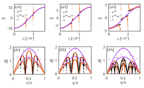
Now we move to the behavior of level spacing. Substituting Eq. S22 into Eq. S14 we see the leading order of level spacing are
| (S23) |
We see that the level spacing is modified by a function dependent on , and could divergence near , but the ratio is a constant for fixed phase. Hence the adjacent gap is almost independent. In Fig. S2(b1)-(b3) we show the level spacing as a function of , we see that the perturbation works well even near the band edge.
.3 The derivation of the average value of
As mentioned in the main text, the sample average of is equivalent to averaging over . We set and suppose . When , and , so
| (S24) |
We observe that the result is consistent with the Poisson distribution, but it is not caused by Poisson statistics.
.4 level statistics of many-body quasiperiodic systems
On the AA model, we introduce nearest-neighbor interactions with a fixed initial phase . From Fig. S3, it can be observed that its level-spacing distribution follows Poisson statistics. Therefore, the localized phases in many-body quasiperiodic systems exhibit Poisson statistics.