Iodine and Bromine Radical Reactions in Atmospheric Mercury Oxidation

Abstract

We investigate the atmospheric oxidation of mercury Hg(0) by halogens, initiated by Br and I to yield Hg(I), and continued by I, Br, BrO, ClO, IO, NO2 and HO2 to yield Hg(II) or Hg(0) using computational methods with focus on determining the impact of rising iodine levels. We calculate reaction enthalpies and Gibbs free energies using the Coupled Cluster singlets, doublets, and perturbative triplets method (CCSD(T)) with the ma-def2-TZVP basis set and effective core potential to account for relativistic effects. Additionally, we investigate the reaction kinetics using variational transition state theory based on geometric scans of bond dissociations at the CASPT2/ma-def2-TZVP level. We compare the results obtained from the CASPT2 and CCSD(T) methods to help define the uncertainty. Our results provide insights into the mechanisms of these reactions and their implications for mercury depletion events and for the atmosphere as a whole. The reaction $\cdot$HgBr + Br$\cdot$ → HgBr₂ was found to be twice as fast as HgI$\cdot$ + I$\cdot$ → HgI₂, with reaction rate coefficients of 8.8$\times 10^{-13}$ and 4.2$\times 10^{-13}$ cm³molecule^-1s^-1 respectively. The BrHg$\cdot$ + Br$\cdot$O → BrHgOBr reaction was about 7.2 times faster than the $\cdot$HgI + IO$\cdot$ → IHgOI reaction with their rates being 3.3$\times 10^{-14}$ and 4.6$\times 10^{-15}$ cm³molecule^-1s^-1 respectively. We investigate the HgXOY (X and Y=halogen) complexes. We find that rising iodine levels will lead to shortened mercury lifetime due to the impact of the HgI$\cdot$ + I$\cdot$ → HgI₂ reaction.

I Introduction

In this paper we use computational methods to investigate the chemical interactions of mercury with bromine and iodine in the atmosphere, focusing in particular on the areas around the poles and Arctic Mercury Depletion Events (AMDEs). Interest in halogens reacting with mercury is driven by their role in promoting the oxidation of Hg to Hg(II) during AMDEs, leading to mercury depostion to the surface. Research focus has mainly been on the reactions between Br$\cdot$ and Hg.[1, 2, 3, 4] It has been suggested that iodine could also play an important role, as an oxidant or by acting to increase the concentration of Br.[5, 6] Due to increasing atmospheric iodine concentrations in the Arctic[7], here we will study the effects of this increase on mercury oxidation and contrast the iodine chemistry with the bromine chemistry. This will be done using computational chemistry to examine the rates of mercury reactions with iodine.

Mercury persists in the atmosphere for about six to eighteen months, which is long enough for it to spread all over the world.[8] Over time, mercury pollution from the populated areas of the Northern Hemisphere reaches the Arctic. In springtime high levels of halogen radicals can be generated photochemically, and tropospheric ozone layer in the Arctic is temporarily depleted and Hg(0) is oxidised.[9] Mercury deposition (and aqueous solubility) increases when it is oxidised, enabling mercury to enter biological ecosystems and rendering them hazardous to humans and animals [4]. Currently, the level of mercury found in the blood of children in areas of the Arctic region is sufficient to cause nerve damage.[10, 11] The mercury level at present is 500 % above its natural atmospheric level [12].

I.1 The atmospheric chemistry of mercury

When entering the atmosphere, the residence time of elemental unoxidized mercury is between 6 and 18 months, which is enough for it to scatter across the Northern Hemisphere [13]. Oxidized mercury, on the other hand, is soluble in water, and its residence time is between hours and days.[14, 6] If the temperature increases by 10 °C, the emitted flux of mercury (either Hg(0) or Hg(CH3)2) increases linking mercury pollution with human activity and climate change.[15, 16, 17]

Globally the main oxidants for Hg(0) are ozone (O₃), generated photochemically [18, 19], hydroxyl radicals, nitrogen oxides (NO_x) and hydrogen peroxide (H₂O₂).[4] The nitrate radical ($\cdot$NO₃) also plays a role at night.[19] While these are the main reactants, in the Arctic atmosphere during springtime, halogen reactions with unoxidized mercury prove to be more significant than the reactions described above. This is due to emissions of halogen compounds and radicals into the atmosphere and at the atmospheric boundary layer of seawater, snow, and ice. The halogen reactions occur mainly in sea salt aerosols, particularly in coastal areas.[4, 19] Oxidized mercury is observed in the atmosphere in low concentrations because it readily dissolves into wet surfaces due to its low vapor pressure.[20, 18, 21, 22]

I.2 Halogen reactions in the atmosphere

The production of reactive halogen species radically changes chemical processes in the Arctic atmospheric boundary layer upon the return of sunlight in the polar spring.[23, 9] A rapid drop in ozone from 30-40 ppb down to 10 ppb has been observed during springtime ozone depletion events in the Arctic.[24, 25] A correlation between bromine and ozone suggested the catalytic destruction of ozone by bromine atoms, [26] but modeling suggests this reaction is not fully understood, and other halogens’ reactivities are not adequately known.[27] Intriguingly, Spolaor et al. found that Hg and I are correlated with each other and with sunlight, while Br did not show a diurnal cycle.[28] Initial observations of inorganic bromine (Br₂, BrO$\cdot$, HOBr), [23] in the polar region have later been updated with the findings of inorganic chlorine (Cl₂, ClO$\cdot$)[29, 30] and iodine (IO$\cdot$, HIO₃).[31, 32] Even if molecular iodine (I₂) has not been previously observed in the Arctic, observations have been made in midlatitude marine and coastal sites,[7] along the Artic and Antarctic coast.[33] Furthermore, IO$\cdot$ has been observed in the Antarctic and the sub-Arctic.[34]

Globally, inorganic iodine compounds released from the ocean account for roughly 3/4 of atmospheric iodine. The remaining atmospheric iodine is estimated to come from organoiodine species (e.g., CH₃I, CH₂I₂, etc.).[35, 36] It has been demonstrated in laboratory studies that oceanic emission of hypoiodous acid (HOI) and molecular iodine (I₂) follow the deposition of tropospheric ozone (O₃) on the ocean surface, and therefore including reactions with iodide (I^-) ions.[37, 38] The increase in global ocean iodine emissions may be in response to a human-driven increase in the level of tropospheric ozone during the industrial period and/or due to increasing Arctic sub-ice biological activity in response to climate change.[39, 40]

I.3 Ice core measurements prove rising iodine levels

As described by Saiz-Lopez et al.,[7] the role of iodine chemistry may increase as the Arctic warms, given the prevalence of iodine chemistry in the marine midlatitudes. Studies of ice cores from Renland on Greenland show that iodine concentrations increased from 1950 to 2010, after being fairly stable from 1750 to 1950. Cuevas[40] attributes the increase of iodine in the ice cores and the atmosphere to human influences - increased tropospheric ozone and recent Arctic warming - leading to an increase in Arctic sub-ice biological activity. An increase in atmospheric iodine levels followed by deposition to ice-covered areas would make local heterogeneous processing and recycling of iodine in ice/snow more efficient, a mechanism supported by recent measurements in the Arctic.[41, 42] Remarkably, from 1990 to 2011, iodine concentrations increased despite stable atmospheric ozone concentrations.[40] Mole fractions $x$(IO) of 1.5 ppt were observed at Alert, Canada in 2015 [31]. Particle formation arising from ppt ($\sim 10^{-12}$) levels of reactive iodine species such as iodic acid (HIO₃) has been observed in the Arctic.[32] These observations, combined with the difficulty of performing laboratory experiments and theoretical investigations with these elements, underscore the need for additional work to characterize iodine’s impact on mercury deposition.[34]

There is also circumstantial evidence suggestive of iodine’s role. In the Arctic saline snowpack, photochemical reactions have been demonstrated involving Br₂, Cl₂ and BrCl.[43, 44, 30] Photochemical reactions with these species have also been shown in laboratory experiments.[45, 46, 47, 48, 49, 50, 51, 52] Further, it has been shown that I₂ and triiodide (I₃^- ) can be photochemically produced in Antarctic snow spiked with iodide (I^-) (1–1,000 $\mu$M).[42] It has also been shown that iodate (IO₃^-) can be photochemically active in frozen solutions.[53] The referenced studies suggest the probability of photochemical production of I₂ is similar to that of Br₂, Cl₂, and BrCl in the Arctic snowpack.[43, 30, 34] Therefore, this article will aim to investigate rates of atmospheric reactions between mercury and iodine and help to estimate the impact of rising atmospheric iodine concentrations over the arctic.

In this article, we investigate reactions R1-R3 described below. The reactions are suggested by Schroeder et al.[18] and Jiao and Dibble.[2]

	Hg + M +X$\cdot$ $\rightarrow$ $\cdot$HgX	(R1)
	$\cdot$HgX + Y$\cdot$ $\rightarrow$ YHgX	(R2)
	$\cdot$HgX + Y$\cdot$ $\rightarrow$ HgXY $\rightarrow$ Hg + XY	(R3)

Here, M is a third body collision partner (N₂, O₂..), and X$\cdot$ = Br$\cdot$, I$\cdot$, and Y = BrO$\cdot$, ClO$\cdot$, IO$\cdot$, $\cdot$NO₂, HO₂$\cdot$, I$\cdot$, or Br$\cdot$. The two last reactions were proposed by Jiao and Dibble as likely propagators in the mechanism. In this article, we focus on reaction chains starting from reaction R1 where X = I$\cdot$ and Br$\cdot$, and the results will be compared with results of X = Br$\cdot$ from other calculations and from literature where this is possible. The goal is to evaluate the extent to which increasing iodine levels in the Arctic will influence AMDEs.

II Method

II.1 Computational Details

In this study we compute reaction energies and reaction rates using the methods of computational quantum chemistry.

The CCSD(T) method with effective core potential (ECP) and a triple zeta basis set is a well-established computational method for calculating reaction energies and properties of mercury at equilibrium geometries.[54, 55] For this project, the specific method used is CCSD(T) with the minimally augmented basis set ma-def2-TZVP, with effective core potentials for relativistic treatment.[56, 54, 55] Previous theoretical investigations of mercury compounds have shown that this method is good for both geometry optimizations and frequency calculations and has been used for accurate calculations on mercury compounds. This is due to the large contribution from the correlation energy compared to that of the contribution of relativistic effects to the energy, though the latter is still significant.

Rate coefficients have been calculated using variational transition state theory.[57] Relaxed geometry scans of the dissociation reactions were performed using CASSCF and the same ma-def2-TZVP basis set to obtain energies and frequencies at intermediate geometries, as input for the variational transition state theory. Preliminary calculations at the unrestricted CCSD(T) level gave many spurious results at intermediate geometries due to spin-contamination, forcing us to employ a proper multi-configurational approach. CASPT2 single-point energy calculations were performed on the geometries, again with the ECP - ma-def2-TZVP basis set. Frequency calculations were performed using either the CASPT2 or CASSCF method with ZORA for the relativistic approximation and ZORA-TZVP basis set. It was necessary to use the ZORA relativistic approximation since the ECP approximation gave results that gave many imaginary frequencies. About 47 intermediate single point energy calculations with the CASPT2/ma-def2-TZVP level of theory and frequency calculations were carried out on the same geometries with the CASPT2 or CASSCF method and ZORA-TZVP basis set. All electronic structure calculations were carried out with the ORCA program.[58, 59, 60] Input files for the calculations in Orca and Ktools can be found in the supplementary Information Section 3.1.

II.2 Kinetics

Variational transition state theory (VTST) was chosen because the mechanisms underlying the reactions between mercury and bromine or iodine radicals have a unique characteristic in that all the investigated reactions only have a reaction barrier when excited rotational and vibrational states are taken into account. The Multiwell program suite was used to carry out the VTST calculations.[61] Multiwell uses the subprogram Ktools for unimolecular dissociation reactions with rovibrational reaction barriers taken into account. From Ktools, the high-pressure rate coefficients for the unimolecular dissociation reaction are given by equation (1). The high-pressure rate coefficients the for reverse reaction in association reactions are calculated using the equilibrium constant relation.

II.2.1 Angular momentum resolved microcanonical VTST in Ktools.

The formulation used in this study is based on the one used in the Multiwell program package.[61, 62] All relevant equations are detailed in the manual, primarily in the sections describing the theory behind Ktools (p. 114) and sctst (p. 209) subprograms. Equation (1) outlines the method for calculating rate coefficients in Ktools for uni-molecular dissociation reactions, averaged over the electronic, vibrational and rotational energy at a specific temperature.

$$k\left(T\right)=\frac{\sum_{J=0}^{J_{\mathit{max}}}\int_{\epsilon=0}^{{\infty}}N^{{{\ddagger}}}\left(\epsilon,J\right)\exp[-\left(\epsilon+E_{\mathit{VT}}+B_{\mathit{VT}}^{+}{\left(J+1\right)}\right)/k_{B}T]\mathit{d\epsilon}}{h\sum_{J=0}^{J_{\mathit{max}}}\int_{\epsilon=0}^{{\infty}}\rho\left(\epsilon,J\right)\exp[-\left(\epsilon+E_{0}+B_{R}^{+}{J\left(J+1\right)}\right)/k_{B}T]\mathit{d\epsilon}}$$ (1)

Above, $E$₀ and $E$_VT denote the potential energies of the reactant and of the variational transition state respectively. The summations are over the angular momentum denoted by quantum number J and the integrals are over the energy $\epsilon$. Where $\epsilon$ is used to define a bundle or interval of energy levels of the total rovibrational energy E⁺ used in the numeric integration, and it is set as a user-defined parameter in Ktools to increase precision or decrease the size of integrals. B_VT and B_R are the rotational constants for the variational transition state and the reactant, respectively.

Before using the expression, the reaction path is analysed. Each reaction coordinate on the reaction path (See Figure 2) is treated as a potential transition state. One or more reaction coordinates are identified as local reaction rate minima. If multiple reaction rate minima or bottlenecks are deemed ”significant”, the transition states are combined to create a ”unified rate coefficient” using Miller’s unified statistical theory.[63, 62]

III Results

III.1 Geometries and Thermodynamics

We performed geometry optimization and frequency calculations at the CCSD(T) level for the molecules investigated in this study. Reaction geometries and harmonic frequencies can be found in the supplementary material section 1. The Gibbs free energy was determined for each molecule investigated here.

III.1.1 Reaction R1 with X = Br or I

The first reaction step, creating the Hg(I) intermediate with iodine or bromine, is similar for the two reactions and is strightforward to compare. The only geometric difference is the bond length in the $\cdot$HgX radicals that differs by 8% (0.22 Å). This also results in a change in frequency of 1.12 cm^-1.

There is also a difference in the reaction of Gibbs free energy between the reaction of Hg+I$\cdot$ (-5.17 kcal/mol) and Hg+Br$\cdot$ (-10.52 kcal/mol). The difference between the two reactions is thus -5.35 kcal/mol. This is an important difference since it would favor the formation of $\cdot$HgBr radicals over $\cdot$HgI radicals. Geometries and frequencies can be found in the supplementary material section 1.1 Table S1.

III.1.2 Reaction R2 with X = Br or I and Y = Br, I, BrO, ClO, IO, or HO₂

The difference in bond length for HgI₂ and HgBr₂ is 7% (0.19 Å). The XHgY molecules have similar geometries (X=halogen; and Y = BrO, ClO, IO, and HO₂). The difference in bond length for the X-HgOX bond shrinks by about 7% (0.17 Å) when interchanging iodine with bromine in the XHgOX molecules.

Furthermore, there is a general increase of the X-HgOX and XHgO-X bond lengths with an increase of the XHgO{X} halogen and a decrease in bond length for the XHg-OX bond. The increase of atomic number of the same halogen also increases the HgOX bond angle, but the XHgO bond angle changes less than a degree.

The largest difference in bond angles between any of these Hg(II)-products is 3.5 degrees between BrHgOCl and BrHgOI for the XHg-O-X bond angle. The largest difference in bond length is 14% (0.28 Å) between IHgOI and IHgOCl for the XHgO-X bond. In the case of the XHgOOH complexes, IHgOOH and BrHgOOH are very similar in geometry, only differing noticeably in the bond length of the X-HgOOH bond (7% or 0.17 Å). See section 1.3 in the supplementary material Table S5 - S8, S31 - S32.

For XHgOX and HgX₂ the largest energy difference between reactant and product is for the HgBr + Br $\rightarrow$ HgBr₂ reaction with a reaction Gibbs free energy change of -61.09 kcal/mol. The stabilization by the Gibbs free energy change decreases from XHgOI over XHgOBr to XHgOCl and XHgOOH. Here the reaction Gibbs free energy is always less negative for the IHgOX molecules than the BrHgOX molecules. The smallest reaction Gibbs free energy is -25.15 kcal/mol in the case of the IHgOOH reaction. There is an energy difference of between 2.65 and 2.70 kcal/mol when interchanging the Br and I at the $\cdot$ XHg radical in reaction R2. There is a general increase in reaction Gibbs free energy with increasing atomic number of the halogen in $\cdot$OX radical of reaction R2. The reaction Gibbs energy of the formation of BrHgOOH is 2.983 kcal/mol larger than the Gibbs free energy for the reaction producing IHgOOH. The results for reaction R2 can be seen in Table 1.

Table 1: shows the standard reaction Gibbs free energy, $\Delta_{r}G^{\stst}$(298 K), and standard reaction enthalpy, $\Delta_{r}H^{\stst}$(0 K), for reaction R2 for the reactions involving HgX₂ and XHgOX calculated at the CCSD(T)/ECP/ma-def2-TZVP level in this work. X denotes one of the halogens Br or I. All the energies are in kcal/mol.

Reaction R2	X=I		X=Br
	$\Delta_{r}G^{\stst}$(298 K)	$\Delta_{r}H^{\stst}$ (0 K)	$\Delta_{r}G^{\stst}$(298 K)	$\Delta_{r}H^{\stst}$ (0 K)
X$\cdot$ + XHg$\cdot$ → HgX2	-50.40	-60.43	-61.09	-71.00
XHg$\cdot$ + $\cdot$OI → XHgOI	-50.94	-61.63	-53.64	-64.24
XHg$\cdot$ + $\cdot$OBr → XHgOBr	-38.76	-46.14	-41.41	-48.69
XHg$\cdot$ + $\cdot$OCl → XHgOCl	-36.06	-48.98	-38.69	-51.58
XHg$\cdot$ + $\cdot$OOH →XHgOOH	-25.15	-36.04	-28.13	-39.00

III.1.3 Reaction R2 with X = Br or I and Y = NO₂

The X-HgNO₂ reaction path exhibits two intermediates and two transition states.

XHg$\cdot$ + NOO $\rightarrow$ XHgNOO $\rightarrow$ TS1 $\rightarrow$ XHgONO-anti $\rightarrow$ TS2 $\rightarrow$ XHgONO-Syn

These can be understood as an example of reaction R2. In the first step of this reaction pathway, the loan pair in nitrogen binds to mercury and creates the intermediate XHgNO₂. Thereafter, a transition state (TS1) creates a barrier for reaching the anti-conformer XHgONO-anti. Another transition state (TS2) creates a barrier for reaching the syn-conformer XHgONO-syn, see Figure 1.

BrHgNO₂

”TS1”

BrHgONO-anti

TS2

BrHgONO-syn

Figure 1: Show the geometries of the intermediates, transition states and the product for the XHgNOO $\rightarrow$ TS1 $\rightarrow$ XHgONO-anti $\rightarrow$ TS2 $\rightarrow$ XHgONO-Syn reaction. Starting from the geometry of XHgNOO and ending in XHgONO-Syn in the order of the reaction.

Geometries for products and intermediates have been compared to the result from Jiao and Dibble.[56] In Jiao and Dibble’s article, the geometries of stationary points (reactants, products, and well-defined transition states) and points along the minimum energy path for reactions were optimized using the PBE0 density functional with the aug-cc-pVTZ basis set and relativistic effective core potentials and then verified by harmonic vibrational frequency analyses at the same level of theory. The energies of stationary points were refined using the CCSD(T) method in conjunction with the aug-cc-pVTZ basis set. In the present study, the geometries were re-optimizated and harmonic frequencies were calculated with the CCSD(T) method, ECPs and the ma-def2-TZVP basis set.

We investigate (TS1) from Jiao and Dibble,[56] by re-optimizing the PBE0 geometry of the transition state at the CCSD(T) level of theory; only a local minimum is found. The CCSD(T) geometry of this local minimum has a difference of 6.50^∘ for the Br-Hg-NOO bond angle, 5.30^∘ for the XHgO-N-O bon angle, 40.30^∘ for the XHg-N-O(1)O(2) and 35.00^∘ for the XHg-N-O(2)O(1).

In this article, the largest difference in bond length of the same configuration is for TS1, where the difference is 0.25 Å for the XHg-ONO bond and the largest difference in bond angle is 0.9^∘ (XHgO-N-O) for the XHgONO-syn conformers. Further information can be found in the supplementary material section 1.5 Tables S16 - S30.

The relative energies for the reaction’s IHgNO₂ products are similar to those of BrHgNO₂, because the geometries along the reaction path are very similar, see Table 2. Due to the difference in the nature of the local minimum ”TS1” for BrHgONO in the present work compared to Jiao and Dibble,[56] the difference in the Gibbs free energy and the enthalpy for ”TS1” is also different. When using Jiao’s PBE0 geometry as a basis for a frequency calculation the energy difference between TS1 and the reactant for BrHgONO is 13.75 kcal/mol $\Delta_{r}G^{\stst}$(298 K). However, when creating a new transition state optimization at the CCSD(T) level, the energy difference is only 1.38 kcal/mol $\Delta_{r}G^{\stst}$(298 K). TS1 for the IHgONO has an energy difference of 2.47 kcal/mol $\Delta_{r}G^{\stst}$(298 K) when optimized with the CCSD(T) method, though the same problem applies to IHgONO ”TS1”. The highest energy barrier along the reaction path for the BrHgNO₂ and IHgNO₂ complex is TS2 with an energy barrier of 5.93 kcal/mol for BrHgNO₂ and 7.12 kcal/mol for the iodine complex.

Table 2: shows the standard reaction Gibbs free energy, $\Delta_{r}G^{\stst}$(298 K), and standard reaction enthalpy, $\Delta_{r}H^{\stst}$(0 K), calculated at the CCSD(T)/ECP/ma-def2-TZVP level, of the reconfiguration of IHgNOO and BrHgNOO as product of reaction R2. All the energies are in kcal/mol.

Reaction steps	X=I		X=Br
	$\Delta_{r}G^{\stst}$(298 K)	$\Delta_{r}H^{\stst}$(0 K)	$\Delta_{r}G^{\stst}$(298 K)	$\Delta_{r}H^{\stst}$(0 K)
XHg + $\cdot$NOO $\rightarrow$ XHgNOO	-19.42	-30.87	-20.58	-32.80
”TS1”	-16.95	-28.25	-19.20	-30.45
XHgONO-anti	-20.90	-32.15	-22.19	-34.32
TS2	-13.78	-25.24	-15.84	-31.32
XHgONO-Syn	-26.73	-38.05	-28.14	-39.64

III.1.4 Reaction R3 with X = Br or I and Y = OCl, OBr or OI

In the article of Jiao and Dibble,[56] reaction R3 is suggested as proceeding via BrHgOOH and BrHgONO, occuring as van der Waals complexes. In a similar manner, HgXOY (X and Y=halogen) complexes are investigated in the present study.

There is a general increase in bond length between oxygen and the middle halogen (HgX-OY) of 8% (0.16 Å) and a change in the XOY angle from 1.5 to 2 degrees between HgBrOY and HgIOY. Furthermore, there is a general trend that with the increasing atomic number of the halogens for the XHgOY and HgXOY molecules, the bond length and angle increase. When only increasing the atomic number of the end halogen (XHgO{Y} or HgXO{Y}), the bond length at the end of the complexes increases (X-HgOY, Hg-XOY / XHgO-Y, HgXO-Y), and the XHg-O-Y and HgX-O-Y bond angle increases as well, while the XHg-OY and HgX-OY bond length decreases. When the atomic number of the {X}HgOY or Hg{X}OY halogen increases, the XHgO-Y or HgXO-Y bong length also increases, while the (X-HgOY, XHg-OY / Hg-XOY, HgX-OY) bond lengths decrease together with the XHg-O-Y or HgX-O-Y bond angle. Geometries and frequencies can be found in the supplementary material section 1.3.

The largest difference in bond length is between HgBrOI and HgBrOCl of 15% (0.30 Å) for the HgXO-Y bond and the largest difference for the HgX-O-Y bond angle is between HgIOI and HgBrOI (4.6 degrees). The HgXOOH van der Waals complex differs only noticeably in the mercury halogen bond length (11% or 0.35 Å). There is also a small change in the HgXO-O-H bond angles, with a change of 2.23 degrees.

As one would imagine the XHgOY products are more stable than the HgXOY van der Waals complexes. For the IHgOY and HgIOY complexes, the difference in Gibbs free energy is around 22 kcal/mol and for the BrHgOY and HgBrOY complexes the difference is around 31 kcal/mol (Table 3).

Table 3: show the differences in Gibbs free energy, calculated at the CCSD(T)/ECP/ma-def2-TZVP level, between the XHgOY product and the HgXOY van der Waals complex in kcal/mol.

Products – van der Waals complex	$\Delta$G${}^{\stst}$(298 K)
	X=I	X=Br
XHgOI - HgXOI	-22.57	-31.76
XHgOBr - HgXOBr	-22.45	-31.52
XHgOCl - HgXOCl	-22.25	-31.24

The area on the potential energy surface surrounding the van der Waals products appears to be a local minimum when looking at the enthalpy. But when calculating the Gibbs free energy at 298.15 K the local minima changes its characteristics to a saddle point along the minimum energy path. This relative shift in the reaction energy of the van der Waals complexes between enthalpy and Gibbs free energy becomes important for the HgBrOOH and HgBrNOO complexes that change characteristics from minima to energy barriers, see Table 4.

The reactions forming the van der Waals complexes (reaction R3), follow the same trend with less negative reaction Gibbs free energies from HgXOI to HgXOCl, see Table 4. However, because of the characteristics of the HgX-OX bond, the HgBrOX forming reactions have less negative reaction Gibbs free energies than their HgIOX counterparts.

Table 4: shows the standard reaction Gibbs free energy, $\Delta_{r}G^{\stst}$(298 K), and standard reaction enthalpy, $\Delta_{r}H^{\stst}$(0 K), calculated at the CCSD(T)/ECP/ma-def2-TZVP level, for reaction R3 for the reactions involving HgXOY. All the energies are in kcal/mol.

Reaction R3	X=I		X=Br
	$\Delta_{r}G^{\stst}$(298 K)	$\Delta_{r}H^{\stst}$(0 K)	$\Delta_{r}G^{\stst}$(298 K)	$\Delta_{r}H^{\stst}$(0 K)
Intermediate - Reactant (van der Waals complex)
$\cdot$XHg+OI$\cdot$ $\rightarrow$ HgXOI	-28.37	-38.43	-21.88	-31.65
$\cdot$XHg+OBr$\cdot$ $\rightarrow$ HgXOBr	-16.30	-25.97	-9.89	-19.23
$\cdot$XHg+OCl$\cdot$ $\rightarrow$ HgXOCl	-13.81	-23.32	-7.45	-16.65
$\cdot$XHg+$\cdot$OOH $\rightarrow$ HgXOOH	-6.45	-16.50	0.72	-10.34
$\cdot$XHg+$\cdot$ONO $\rightarrow$ HgXNO2	-2.06	-13.18	0.66	-10.94
Product - Intermediate (van der Waals complex)
HgXOI $\rightarrow$ Hg+XOI	-3.93	3.42	-4.92	2.22
HgXOBr $\rightarrow$ Hg+XOBr	-3.79	3.54	-5.79	1.11
HgXOCl $\rightarrow$ Hg+XOCl	-3.66	3.59	-4.64	2.35
HgXOOH $\rightarrow$ Hg+XOOH	—–	—–	-4.54	3.38
HgXNO2 $\rightarrow$Hg+XNO2	-4.87	2.81	-7.15	0.59
Product - Reactant (van der Waals complex)
$\cdot$XHg+OI$\cdot$ $\rightarrow$ Hg+XOI	-32.30	-35.01	-26.80	-29.43
$\cdot$XHg+OBr$\cdot$ $\rightarrow$ Hg+XOBr	-20.09	-22.43	-15.68	-18.12
$\cdot$XHg+OCl$\cdot$ $\rightarrow$ Hg+XOCl	-17.47	-19.73	-12.09	-14.30
$\cdot$XHg+$\cdot$OOH $\rightarrow$ Hg+XOOH	—–	—–	-3.82	-6.96
$\cdot$XHg+$\cdot$ONO $\rightarrow$ Hg+XNO2	-6.93	-10.37	-6.49	-10.35

III.1.5 Reaction R3 with X = Br or I and Y = NO₂ or OOH

It was only possible to find the transition states suggested in the article of Jiao and Dibble[56] for the $\cdot$HgBr + $\cdot$OOH $\rightarrow$ HgBrOOH $\rightarrow$ Hg + BrOOH reaction (R3) at the B3LYP/ECP/ma-def2-TZVP level of theory, but it could not be confirmed at the CCSD(T)/ECP/ma-def2-TZVP level of theory. This transition state should create an energy barrier for the enthalpy at 0 K of 1.6 kcal/mol. The reaction enthalpy for the HgBrOOH ”van der Walls” complex was found to be -10.34 kcal/mol compared to Jiao and Dibble’s -11.9 kcal/mol,[56] see Table 4. When calculating the Gibbs free energy difference between the intermediate and the reactant it was found to be positive, though only by 0.72 kcal/mol. The T1 diagnostics of the HgBrOOH ”van der Walls” complex has a value of 0.014 (less than 0.02) which suggest that the calculation should be well described by the CCSD(T) single reference method.

In the case of HgBrOOH, the van der Waals complex HgBrNOO has a minimum on the potential energy surface for the enthalpy at 0 K, but when investigating the Gibbs energy at 298 K, the energy of the intermediate this is larger than the energy of the reactant by a small margin of 0.66 kcal/mol, see Table 4.

Examining the reaction enthalpy at 0 K, it is seen that the van der Waals intermediate is more stable than the van der Waals product with a reaction barrier to the dissociation product Hg + BrOOH of 3.63 kcal/mol. This changes when compared with the Gibbs free energy in which case the product from the van der Waals complex is lower in energy relative to the van der Waals complex itself. At 298.15 K the difference for the Gibbs free energy is 4.54 kcal/mol.

Unlike to the case of HgBrOOH and HgBrNOO, where the dynamics of the reaction is changed from a positive energy difference to a reaction with a negative energy differnence, the HgINOO and HgIOOH van der Waals complexes only have negative energy differences, in the case of the reaction enthalpy at 0 K (-16.50 kcal/mol) and the Gibbs free energy at 298.15 K (-6.45 kcal/mol) for HgIOOH, or in the case of the reaction enthalpy at 0 K (-13.18 kcal/mol) and the Gibbs free energy at 298.15 K (-2.06 kcal/mol) for HgINOO.

If the reaction R3 for $\cdot$HgX + $\cdot$NO₂ was the only reaction considered, then Hg would be more likely to be reformed in the $\cdot$HgBr + $\cdot$NO₂ reaction than in the $\cdot$HgI + $\cdot$NO₂ reaction. The same would apply to the $\cdot$HgBr + $\cdot$OOH reaction R3. In the other examples of the reversed reaction R3 investigated, this would also hold true, although the formation of Hg would be significantly more irrelevant and unlikely because of the van der Walls intermediates being significantly more stable.

III.2 Kinetics

In the calculation of the reaction rates we have made use of a combination of CASSCF and CASPT2 calculations instead of the CCSD(T) approach employed in the calculation of the reaction energies and Gibbs free energies. Before we will analyse the results of these calculations we will first estimate the accuracy of these calculations by comparing to the CCSD(T) reaction energies.

III.2.1 Estimation of Precision

The parameters that the Ktools program uses to calculate the rate coefficients are the enthalpy at zero Kelvin, the harmonic frequencies, and the rotational constants at many points along the reaction path. Therefore, a comparison between CASPT2 reaction energies extracted from the geometric scans, Figure 2, and CCSD(T) reaction energies, calculated from reactant and product energies, is made in Table 5.

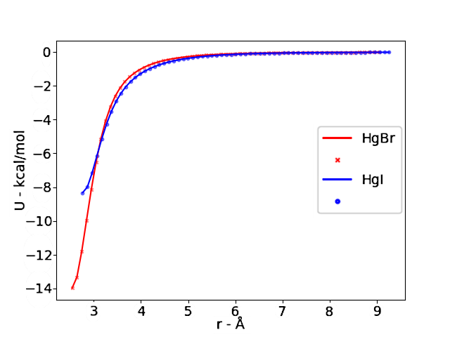
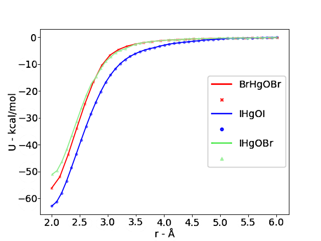
(a) (b)
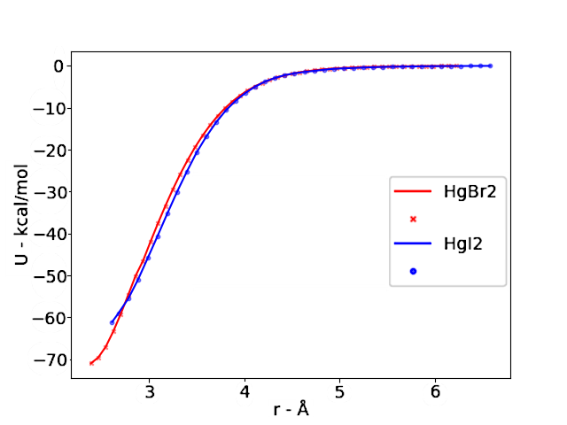
(c) (d)

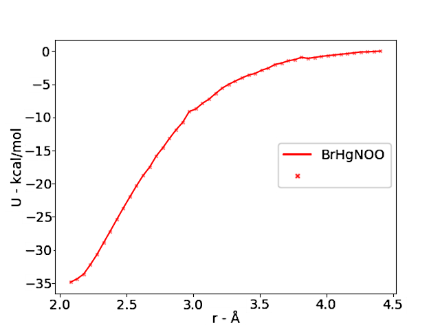
Figure 2: This figure shows the electronic energy in kcal/mol for the dissociation of the bonds of (a) Hg-Br and HgI - (b) IHg-I and BrHg-Br - (c) BrHgOBr, IHgOI and IHgOBr calculated with the CASPT2 method. The active spaces used in (b), (c) and (d) bonds can be found in Table 5. The geometry of (b), (c) and (d) is calculated from CASSCF/ma-def2-TZVP relaxed scans over the dissociating bond.

Table 5: shows electronic reaction energies $\Delta E$ for the dissociation reactions calculated with the CCSD(T) and CASPT2 methods, both with ma-def2-TZVP basis sets. Also, the difference in the electronic reaction energies calculated with the CASPT2 and CCSD(T) methods is shown. All energies are in kcal/mol.

Reaction		$\Delta$E		Difference $\Delta$E
product	active space	CASPT2	CCSD(T)	CASPT2 - CCSD(T)
HgBr2	12e12o	-70.9959	-71.7103	0.7144
HgI2	10e10o	-61.5792	-60.9500	-0.6292
BrHgOBr	10e10o	-56.2394	-54.8740	-1.3654
BrHgOI	12e12o	-57.9194	-66.0154	8.0960
IHgOBr	14e14o	-51.0338	-50.1649	-0.8689
IHgOI	10e10o	-62.8126	-63.3458	0.5332
BrHgNOO	16e13o	-34.8426	-34.2926	-0.5500

The electronic reaction energies calculated by the CASPT2 method with the ma-def2-TZVP basis set differ only slightly from the CCSD(T) electronic reaction energy. The two largest differences between the CCSD(T) and CASPT2 reaction energies are 1.37 kcal/mol for BrHgOBr and 8.10 kcal/mol for BrHgOI. The former is only slightly more than the chemical accuracy of 1 kcal/mol. As a rule of thumb, a difference of the order of the chemical accuracy in the activation energy leads to a factor of 5 in the rate coefficient. Therefore, the kinetic result for the reactions forming BrHgOI might not be as accurate as for the other reactions.

Another source of error concerns the precision of the frequency calculation. Calculating frequencies using the ECP relativistic approximation in the CASPT2 or CASSCF calculations resulted in too many imaginary frequencies. Therefore the ZORA relativistic approximation was used instead at the price of increasing the number of basis functions and thus expanding the size of the calculation. Obviously we cannot compare the ECP and ZORA calculated CASPT2 or CASSCF frequencies. Therefore, in Table 6, a comparison is made between the reaction energy calculated at the ECP CASPT2/ma-def2-TZVP level of theory and the ZORA CASPT2 or CASSCF/ma-def2-TZVP level of theory. This is to give an idea of the uncertainty in these calculations. The largest derivation of the energy is 16% in the case of IHgOI.

Table 6: shows the difference in electronic reaction energy $\Delta E$ (in kcal/mol) between the ECP CASPT2 calculations used for the electronic energy in the kinetic calculations and the ZORA CASPT2 or CASSCF electronic energy used in for the frequency calculation.

CAS method			$\Delta E$
frequency	active space	reaction product	ZORA	ECP	% difference
CASPT2	12e12o	HgBr2	-70.50253	-70.99589	1%
CASSCF	10e10o	HgI2	-59.2838	-61.5792	4%
CASPT2	10e10o	BrHgOBr	-52.7045	-57.8602	9%
CASSCF	14e14o	IHgOBr	-62.1461	-51.0338	10%
CASPT2	10e10o	IHgOI	-52.5597	-62.8126	16%
CASPT2	10e10o	BHgOI	-55.3210	-57.9194	5%

III.3 Rate Coefficient Results

The reaction rates in this study are calculated using the Multiwell program suite and its subprogram Ktools. The energy of the bond-dissociating reactions has been calculated using two different approaches, taking into account the distinct behavior of monoradical and biradical reactions. For reaction R1 calculations can be carried out using single reference methods, in this case CCSD(T). However, the energy for bond-breaking reactions forming biradicals is not described accurately at the CCSD(T) level of theory (reaction R2). Therefore, it has been necessary to use CASPT2 to accurately describe the dissociation energy,[64] although CCSD(T) reaction energies calculated from the equilibrium geometries of the product and reactants have been relied upon for comparison, Table 5. More information about the specifics of the CAS calculations can be found in the next section, and the input files for these calculations can be found in the supplementary material section 3.1.

This article focuses on the difference between the reaction rates of iodine and bromine species. The kinetics of the reactions generally follow the trend as expected from the reaction energies, as can be seen in Table 7. The reactions containing bromine are generally faster. When comparing the formation of HgBr₂ and HgI₂ in reaction R2, there is a difference making the reaction forming HgBr₂ twice as fast as the reaction forming HgI₂. Furthermore, the reaction forming BrHgOBr is about 7.2 times faster than the one forming IHgOI, about 6.5 times faster than that forming IHgOBr and about 10 times faster than that forming BrHgOI.

Table 7: shows the rate coefficients in cm³molecule^-1s^-1 for a selection of the dissociation reactions of reaction R1 and R2. The rates have been calculated using the the program Ktools. Electronic energies for reaction R1 have been calculated using ECP CCSD(T)/ma-def2-TZVP. Electronic energies for biradical reaction R2 containing have been calculated using ECP CASPT2/ma-def2-TZVP, and frequencies have been calculated using ZORA CASPT2 or CASSCF/ZORA-TZVP.

Reactions		R1		R2
Product		$\cdot$HgBr	$\cdot$HgI	HgBr2	HgI2	BrHgOBr	IHgOI	IHgOBr	BrHgOI
Rate in		3.3$\times$10-13	5.5$\times$10-13	8.8$\times$10-13	4.2$\times$10-13	3.3$\times$10-14	4.6$\times$10-15	5.1$\times$10-15	3.3$\times$10-15
cm3molecule-1s-1

Table 8: This table shows rate coefficients from the literature in cm³molecule^-1s^-1.

Reaction	rate coefficients		Reference
Hg+I$\cdot$→$\cdot$HgI	4.00$\times$10-13	B3LYP/RRKM	Skov 2004 [4]	theory
Hg + I2 → HgI2	1.27 (±0.58) $\times$10-19		Raolfie 2008 [65]	exp.
Hg+Br$\cdot$→HgBr	3.70$\times$10-13	CCSD(T)/RRKM	Goodsite 2012 [66]	theory
	9.8$\times$10-13	Quas-CT	Shepler 2007 [67]	theory
	6.4(±.2)$\times$10-13		Sumner 2011 [68]	exp.
$\cdot$HgBr+Br$\cdot$→HgBr2	2.50$\times$10-10	B3LYP/RRKM	Skov 2004 [4]	theory
	3.0(±0.1)$\times$10-11	MRCI/Quasi-CT	Balabanov 2005 [69]	theory
	7.00$\times$10-17	at 397 K	Greg 1970 [70]	exp.
Hg+Br2→HgBr2	2.8$\times$10-31	MRCI/	Balabanov 2005 [69]	theory
		microcanonial VTST
	9$\times$10-17		Ariya 2002 [71]	exp.
Hg+BrO$\cdot$→HgBrO	(3.0–6.4)$\times$10-14		Spicer 2002 [72]	exp.
	(1–100) $\times$10-15		Raofie 2004 [73]	exp.
$\cdot$HgBr+$\cdot$NO2→BrHgONO	8.14$\times$10-11	PBE0//	Jiao 2017 [56]	theory
		RCCSDT/QuasCT
Hg+$\cdot$NO3→HgO+$\cdot$NO2	<4$\times$10-15		Sommar 1997 [74]	exp.
	<7$\times$10-15		Sumner 2005 [75]	exp.
Hg+Cl$\cdot$→HgCl$\cdot$	5.40$\times$10-13		Donohoue 2005 [76]	exp.
	2.80$\times$10-12	CCSD(T)/CVTST	Khalizov 2003 [54]	theory
Hg+ClO$\cdot$ → HgClO$\cdot$	1.1$\times$10-11		Byun 2010 [77]	exp.
	3.6$\times$10-17		Spicer 2002 [72]	exp.
Hg+Cl2 → HgCl2	2.6(±0.2)$\times$1018		Ariya 2002 [71]	exp.
	2.5(±0.9)$\times$10-18		Sumner 2005 [75]	exp.
Hg + HCl → HgCl2 + H	1.50$\times$10-33	QCISD	Wilcox 2003 [78]	theory
	1.00$\times$10-19		Hall 1993 [79]	exp.
Hg+F→HgF	1.86$\times$10-12	CCSD(T)/CVTST	Khalizov 2003 [54]	theory
Hg+$\cdot$OH→HgOH	9.0(±1.3)$\times$10-14		Pal 2004 [80]	exp.
	8.7(±2.8)$\times$10-14		Sommar 1997 [74]	exp.
HgOH+O2→HgO+OH	3.2$\times$10-13	B3LYP/RRKM	Skov 2004 [4]	theory
	9.0(±1.3)$\times$10-14		Pal 2004 [80]	exp.
Hg+O2→HgO+O2	7.5(±0.9)$\times$10-19		Pal 2004 [81]	exp.
	3.1$\times$10-40	QCISD(T)//	Xu 2008 [82]	theory
		MP2/TST
Hg + H2O2 → HgO +H2O	${\leq}$4.1$\times$10-16		Seigneur 1994 [83]	exp.
	<8.5$\times$10-19	293 K	Tokos 1998 [84]	exp.
$\cdot$HgBr + $\cdot$OOH → BrHgOOH		PBE0//	Jiao 2017 [56]	theory
	3.51$\times$10-11	RCCSDT/QuasCT

IV Discussion

IV.1 Comparison with literature rate coefficients

Where possible, the rate coefficients calculated in this study by Ktools are compared with the rate coefficients presented in the literature. The values of the rates of reaction R1: X$\cdot$ + Hg → $\cdot$HgX are in good agreement with the values shown in Table 8. They only differ slightly, with a factor of 0.89 for the reaction containing bromine and a factor of 1.38 for the reaction containing iodine compared to calculations made by Goodsite[66] and Skov.[4]

The forward rate coefficients given here are calculated by Ktools as the reverse rate coefficient divided by the equilibrium constant. When the reverse rate coefficient for reaction R2: HgBr₂ → Br$\cdot$ + $\cdot$HgBr is compared with the one calculated by Balabanov et al.[69] (5.5$\times$10^-39 s^-1), the reverse rate coefficient calculated in this study (3.5$\times$10^-39 s^-1) differs only by a factor of 0.63. The equilibrium constant given in Balabanov’s article is 5.407325$\times$10^-27 molecule$\cdot$cm^-3, which differs by only a factor of 1.4 from the equilibrium constant calculated in this study 3.9$\times$10^-27 molecule$\cdot$cm^-3. The forward rate coefficient given in Balabanov’s article is 3.0$\times$10^-11 cm³molecule^-1s^-1. The difference between the forward rate coefficient calculated in this study (8.8$\times$10^-13 cm³molecule^-1s^-1) and the forward rate coefficient from Balabanov’s article would then differ by a factor of 34. However, if a forward rate coefficient is calculated as the reverse rate coefficient divided by the equilibrium constant, both from Balbanov’s article [69], the result is 1.017$\times$10^-12 cm³molecule^-1s^-1, which differs from the one calculated by Ktools only by a factor of 1.16. The rate coefficients calculated here are all calculated using the same approach, and are therefore suitable for the comparisons presented here.

The most influential difference of the result in this article is the result of reaction R2: X$\cdot$ + $\cdot$HgX $\rightarrow$ HgX₂, both because the rate of the reaction is the fastest calculated in this study and due to the similarities of the rates for the reactions, including bromine and iodine. The rate of reaction R2, including bromine, is close to the rate of the $\cdot$HgBr+$\cdot$NO₂→BrHgONO reaction with a rate of 8.1$\times$10^-11 cm³molecule^-1s^-1 and the $\cdot$HgBr+$\cdot$OOH→BrHgOOH reaction with a rate of 3.5$\times$10^-11 cm³molecule^-1s^-1 see Table 9.

Table 9: presents the relative reaction rates are calculated by dividing the rate of the left dissociation reaction (in which a bromine atom in the dissociating molecule is replaced by an iodine atom) by the rate of the right dissociation reaction.

Br	Rate		I	Rate		Relative
species	cm3molecules-1s-1		species	cm3molecules-1s-1		Rate
HgBr2	8.8$\times$10-13	devided by	HgI2	4.2$\times$10-13	=	2.09
BrHgOBr	3.3$\times$10-14	devided by	IHgOI	4.6$\times$10-15	=	7.20
BrHgOBr	3.3$\times$10-14	devided by	IHgOBr	5.1$\times$10-15	=	6.53
BrHgOBr	3.3$\times$10-14	devided by	BrHgOI	3.3$\times$10-15	=	10.0
IHgOBr	5.1$\times$10-15	devided by	IHgOI	4.6$\times$10-15	=	1.10
IHgOBr	5.1$\times$10-15	devided by	BrHgOI	3.3$\times$10-15	=	1.53
IHgOI	4.6$\times$10-15	devided by	BrHgOI	3.3$\times$10-15	=	1.39

For reaction R2: (OX$\cdot$ + $\cdot$HgX $\rightarrow$ XHgOX) the rate of the reactions is in the range between 3.3$\times$10^-14 - 3.3$\times$10^-15 cm³molecule^-1s^-1. The rate coefficient is about 7.2 times higher for reaction R2 including BrHg$\cdot$ and $\cdot$OBr than the one including IHg$\cdot$ and $\cdot$OI. The rate coefficients for reactions forming the products IHgOI, IHgOBr and BrHgOI do not largely differ. The rates for the reaction BrO$\cdot$ + $\cdot$HgBr $\rightarrow$ BrHgOBr have about 12.7 times smaller rate coefficient as IHg$\cdot$ + I$\cdot$ $\rightarrow$ IHgI. Since the concentrations of $\cdot$OBr would generally be assumed larger than the concentration of I radicals, the BrHgOBr reaction R2 could be significant compared with the reaction forming IHgI. The concentration of the OI$\cdot$ species must be about 10 times higher than that of the OBr$\cdot$ radicals to compete and up to 18 thousand times higher than $\cdot$NO₂, $\cdot$OOH, and Br$\cdot$ to compete with their reaction rates of the $\cdot$HgBr+$\cdot$NO₂$\rightarrow$BrHgONO, $\cdot$HgBr+$\cdot$OOH$\rightarrow$BrHgOOH, and Br$\cdot$ + $\cdot$HgBr $\rightarrow$ HgBr₂ reactions.

To further the understanding of how iodine competes with bromine reactions in the atmosphere the reactions of $\cdot$HgI+$\cdot$NO₂→IHgONO and $\cdot$HgI+$\cdot$OOH→IHgOOH need further investigation. From reaction energies, the bromine reactions would be favored over the iodine reactions, but certainty cannot be established without further investigation of the kinetics.

From the literature, Table 8, there are known reactions, including halogens and mercury that have rate coefficients in a range faster than BrHg$\cdot$ + $\cdot$OBr $\rightarrow$ BrHgOBr (3.3$\times$10^-14cm³molecule^-1s^-1). These are:
Hg + $\cdot$OBr $\rightarrow$ HgOBr Hg + $\cdot$Cl $\rightarrow$ HgCl Hg + ClO$\cdot$ → HgClO Hg + F$\cdot$ → HgF$\cdot$
Relevant reactions of the same rate that do not include halogen are the reactions:
Hg + $\cdot$OH → HgOH HgOH + $\cdot$O₂→HgO(s) + $\cdot$OH

Because the overall rate of the reactions is dependent both on the rate coefficient and the atmospheric concentrations of the chemical species, a brief estimate of the mixing ratio in the Arctic and Antarctic is presented in the next section.

IV.2 Atmospheric Mixing Ratios in the Arctic and Antarctic

When looking at the atmospheric concentrations, high maximum mixing ratios of bromine, chlorine, and iodine species have been measured at depletion events both in the Arctic and in the Antarctic. Here maximum concentrations of BrO$\cdot$, IO$\cdot$, and ClO$\cdot$ radicals have been measured up to 50 ppt,[85] 30 ppt,[86] and 44 ppt.[87] It is hard to compare these maximum concentrations, since they are all measured from single or rarely occurring episodes. At a few locations, atmospheric concentrations of two or three halogen monoxides have been measured at the same time and place. Saiz-Lopez et al.[88] made measurements of BrO$\cdot$ and IO$\cdot$ at Hally Bay in the Antarctic and reported similar mixing ratios of BrO$\cdot$ and IO$\cdot$ with maximums of 20.2 and 20.5 ppt and minimums of both below the detection limit of 2 ppt.

In the dissertation of Zielcke,[31] there are reports of rare events with mixing ratios of BrO$\cdot$ over 20 ppt. In the Arctic in 2014, average measurements were made and compared with the solar zenith angle (SZA) with values from 5 ppt (SZA[-85]) in the spring dropping to 1 ppt (SZA[-45]) in the summer and rising again to about 5 ppt in the fall. In the Antarctic, BrO$\cdot$ mixing rate was reported over the year with the result of mixing ratios raising from below the detection limit to 3 ppt in the spring (SZA [-90 to -80]), falling again in the summer to 1 ppt and rising to 1.5 ppt in the fall, before dropping to back below the detection limit in the winter.

In the same series of measurements, IO$\cdot$ was measured in the Arctic ranging from 0.1 ppt (SZA[90]) spring to 0.3 ppt (SZA[50]) summer. In the Antarctic, the average ranges from 0.35 ppt spring to 0.15 ppt in summer and back to about 0.35 ppt in the fall.[31]

$\cdot$NO₂ in the Arctic dropped from 0.2 ppb in the spring to under the detection limit in the summer, rising again to 0.2 ppb in the fall. In the Antarctic, the mole fraction rises to 1.3 ppb in the spring, dropping below the detection limit in the summer, and rises up back over 1 ppb in the fall.[31]

During the SOLVE[89] science flights over the Norwegian Sea near the Arctic, the atmospheric concentrations of $\cdot$HO₂, ClO$\cdot$, and $\cdot$NO₂ radicals were measured with average concentrations in clouds of 0.36 ppt, 20.1 ppt, and 24 ppt. In cloud-free surroundings, the measurements were 0.25 ppt, 11.8 ppt, and 18.4 ppt. From fall to winter, $\cdot$HO₂ concentrations fall from about 2 ppt to about 0.1 ppt. ClO$\cdot$ radicals falls from about 30 ppt to about 10 ppt. Reasons for the difference in $\cdot$NO₂ mixing ratios compared to Zielcke[31] can be due to local factors such as maritime traffic in the Norwegian Sea.

The average concentrations of $\cdot$OH during the SOLVE mission was 0.026 ppt and was dropping from fall to winter from about 0.1 ppt to about 0.01 ppt.[89]

Few measurements are available concerning the concentrations of the atomic radicals. The only example of the atomic iodine radical $\cdot$I found in literature was measured at Mace Head in Ireland. There measured mixing ratios ranging from under the limit of detection (5.3 ppt) up to 22 ppt were detected on 29 Aug 2007.[90] Atomic chlorine radicals have been estimated to go up to concentrations of about 0.05 ppt.[87] The concentration of atomic bromine radicals measured in Borrow Alaska by Wang et al.[91] ranged from 4 ppt to 14 ppt over an Ozone Depletion Event, with measured Br$\cdot$/BrO$\cdot$ ratios ranging from 7.5 during an Ozone Depletion Event to more normal levels of 0.1.

Local conditions vary widely, and the atmospheric concentration of halogen radicals have a significant effect on the AMDE. From Tables 10 and 11 we can only get a partial understanding of these concentrations, making it even harder to predict how external factors such as global warming will change these conditions. There is substantial evidence to suggest that iodine concentrations may rise due to global warming. However, the reactions investigated in this study indicate that the radical species of Br$\cdot$ and $\cdot$OBr are the primary contributors. Should iodine species, such as atomic iodine, become more abundant than concentrations of atmospheric bromine species - contrary to current observations - iodine could then compete with bromine in atmospheric reactions during the mercury depletion events. Iodine will also play a role in activating bromine [5]. In this context, it is mainly atomic iodine radicals that will be competitive, whereas $\cdot$OI radicals would need to be substantially more abundant to compete effectively. Based on these observations, we can resolve that the AMDEs are dependent on the concentration of the radical species, and the role of iodine species as contributors therefore cannot be ruled out.

Table 10: The maximum concentrations used for comparison of the calculated rate coefficients calculated.

Species	Maximum	Location		Ref.
	mixing ratio ppt
BrO$\cdot$	50	Polarstern	Antarctic	Wagner 2007 [85]
	20	Alert Base	Arctic	Zielcke 2015 [31]
	20	Halley Bay	Antarctic	Saiz-Lopez 2015 [41]
IO$\cdot$	30	Mace Head	Ireland	Commane 2011 [86]
	20	Halley Bay	Antarctic	Saiz-Lopez 2007 [88]
	3.4	Hudson’s Bay	Arctic	Mahaja 2010 [92]
	0.8	Svalbard	Arctic	Wittrock 2000 [93]
ClO$\cdot$	44	Barrow	Alaska	Custard 2016 [87]
Br$\cdot$	14	Barrow	Alaska	Wang 2019 [91]
I$\cdot$	22	Mace Head	Ireland	Bale 2008 [90]

Table 11: show the average concentration used for comparison of the calculated rate coefficients calculated.

Species	Average yearly variations ppt	location	region	reff.
BrO$\cdot$	5 - 2	Alert Base	Arctic	Zielcke 2015 [31]
	3 - 1	Scott Base	Antarctic	Zielcke 2015 [31]
IO$\cdot$	0.3 - 0.1	Alert Base	Arctic	Zielcke 2015 [31]
	0.35 - 0.15	Scott Base	Antarctic	Zielcke 2015 [31]
ClO$\cdot$	30 - 10	SOLVE	Arctic	Simpas 2012 [89]
HO2$\cdot$	2 - 0.1	SOLVE	Arctic	Simpas 2012 [89]
NO2	0.0002 - LOD	Alert Base	Arctic	Zielcke 2015 [31]
	0.0013 - LOD	Scott Base	Antarctic	Zielcke 2015 [31]
$\cdot$OH	0.1 - 0.01	SOLVE	Arctic	Simpas 2012 [89]

V Conclusion and Outlook

The study conducted provides an analysis and comparison of calculated reaction energies and rate coefficients of mercury’s reactions with bromine and iodine, particularly in the context of atmospheric concentrations over the Arctic. Utilizing the ORCA quantum chemistry program, the reaction energies were calculated at the CCSD(T) level while the reaction scans were carried out at the CASSCF/CASPT2 level, from which the reaction rates were calculated with the Ktools program. CASPT2 calculations of bond dissociation energies were compared to corresponding CCSD(T) energies and the rate coefficients were compared with literature where possible.

The following observations emerge for the reaction energy. The reactions with the largest stabilization of Gibbs free energy creating Hg(II) from reaction R2 ($\cdot$XHg +Y$\cdot$ $\rightarrow$ XHgY) are the reaction forming HgBr₂ with a stabilization energy of 61.09 kcal/mol.

The stabilization by the Gibbs free energy decreases with increasing atomic number, from XHgOI over XHgOBr to XHgOCl. Furthermore, at the other end of the series of molecules, IHgOX molecules are consistently less stable than their BrHgOX counterparts. The least stable XHgOX-product is IHgOCl with a stabilization of 36.06 kcal/mol in Gibbs free energy.

Lower stabilizing reaction Gibbs free energies are observed for the reactions forming XHgOOH and XHgNOO, where the former is more stable than the latter. The reaction forming IHgNOO has the lowest energy difference among the $\cdot$XHg +Y$\cdot$ $\rightarrow$ XHgY reactions.

The following observations emerge concerning the rate of the reactions. The derived rate coefficients (X=Br $3.3\cdot 10^{-13}$ & X=I $5.5\cdot 10^{-13}$ cm³molecule^-1s^-1) for the reaction X$\cdot$ + Hg $\rightarrow$ $\cdot$HgX, were found to be consistent with the literature values, underlining the validity of the computational approach.

For reaction R2, the reverse rate and the equilibrium constant were found in agreement with Balabanov et al.[69] A dissimilarity was noted in the forward rate coefficient when compared to Balabanov et al. However, the comparison of the rate coefficients in this article should be reliable, as all have been calculated with the same approach.

The most significant difference between iodine and bromine reaction rates was for reaction R2. The bromine-containing forward reaction rate coefficient ($k$= 8.8$\times$10^-13 cm³molecule^-1s^-1) was calculated to be twice as fast as its iodine counterpart, with a rate of 4.2$\times$10^-13 cm³molecule^-1s^-1. Calculated reaction rates for reaction R2 ($\cdot$XHg +OX$\cdot$ $\rightarrow$ XHgOX ) differed in their forward rate coefficients and were between 3.3$\times$10^-14 and 3.3$\times$10^-15 cm³molecule^-1s^-1. The reaction R2 forming BrHgOBr was about 7.2 times faster than the one forming IHgOI, about 6.5 times faster than the one forming IHgOBr, and about 10 times faster than the one forming BrHgOI.

Atmospheric concentrations of the chemical species of halogen radicals are strongly correlated with local conditions. The general understanding is that there is a larger mixing ratio of bromine radical species in the atmosphere over the Arctic and Antarctic than iodine radical species. Iodine, bromine, and chlorine radicals are implicated in depletion events globally, depending on local conditions.

In accordance of the findings outlined earlier, the reactions between mercury and iodine are not likely to dramatically alter the overall rates of atmospheric reactions involving mercury. This is due to the reactions between mercury and iodine not being faster than those reactions involving bromine, which remains the dominant atmospheric reactant for mercury during springtime in the Arctic and Antarctic. Additionally, the mixing ratio of iodine radical species in the Arctic atmosphere is not greater than that of bromine radical species. These observations reinforce the idea that bromine is the primary atmospheric reactant influencing mercury in the Arctic, Antarctic, and in atmospheric mercury depletion events (ADME). Based on these observations, we can conclude that the AMDEs are dependent on the concentration of these radical species, and the role of iodine species as potential contributors cannot be ruled out. A significant increase in atmospheric concentrations of iodine over the Arctic and Antarctic would only have a substantial impact on mercury’s atmospheric reactions if the atmospheric mixing ratio of iodine markedly surpassed those of atmospheric bromine.

References

- Dibble, Zelie, and Mao [2012] T. S. Dibble, M. J. Zelie, and H. Mao, “Thermodynamics of reactions of ClHg and BrHg radicals with atmospherically abundant free radicals H,” Atmospheric Chemistry and Physics 12, 10271–10279 (2012).
- Jiao and Dibble [2015] Y. Jiao and T. S. Dibble, “Quality Structures, Vibrational Frequencies, and Thermochemistry of the Products of Reaction of BrHg• with NO2, HO2, ClO, BrO, and IO,” The Journal of Physical Chemistry A 119, 10502–10510 (2015).
- Horowitz et al. [2017] H. M. Horowitz, D. J. Jacob, Y. Zhang, T. S. Dibble, F. Slemr, H. M. Amos, J. A. Schmidt, E. S. Corbitt, E. A. Marais, and E. M. Sunderland, “A new mechanism for atmospheric mercury redox chemistry: implications for the global mercury budget,” Atmospheric Chemistry and Physics 17, 6353–637 (2017).
- Skov et al. [2004] H. Skov, J. H. Christensen, M. E. Goodsite, N. Z. Heidam, B. Jensen, and P. Wåhlin, “Fate of elemental mercury in the arctic during atmospheric mercury depletion episodes and the load of atmospheric mercury to the arctic. antarctic springtime depletion of atmospheric mercury,” Environmental Science & Technology 38, 2373–2382 (2004).
- Calvert and Lindberg [2004] J. G. Calvert and S. E. Lindberg, “The potential influence of iodine-containing compounds on the chemistry of the troposphere in the polar spring. ii. mercury depletion,” Atmospheric Environment 38, 5105–5116 (2004).
- Ariya et al. [2008] P. A. Ariya, H. Skov, M. M. L. Grage, and M. E. Goodsite, “Gaseous Elemental Mercury in the Ambient Atmosphere: Review of the Application of Theoretical Calculations and Experimental Studies for Determination of Reaction Coefficients and Mechanisms with Halogens and Other Reactants,” Advances in Quantum Chemistry 55, 43–55 (2008).
- Saiz-Lopez et al. [2012] A. Saiz-Lopez, J. M. C. Plane, A. R. Baker, L. J. Carpenter, R. von Glasow, J. C. Gómez Martín, and R. W. Saunders, “Atmospheric chemistry of iodine,” Chemical Reviews 112, 1773–1804 (2012).
- Subir, Ariya, and Dastoor [2011] M. Subir, P. Ariya, and A. Dastoor, “A review of uncertainties in atmospheric modeling of mercury chemistry. uncertainties in existing kinetic parameters - fundamental limitations and the importance of heterogeneous chemistry,” Elsevier Ltd , 04. 046 (2011).
- Steffen et al. [2008] A. Steffen, T. Douglas, M. Amyot, P. Ariya, K. Aspmo, T. Berg, J. Bottenheim, S. Brooks, F. Cobbett, A. Dastoor, et al., “A synthesis of atmospheric mercury depletion event chemistry in the atmosphere and snow,” Atmospheric Chemistry and Physics 8, 1445–1482 (2008).
- Ethier et al. [2012] A. Ethier, G. Muckle, C. Bastien, E. Dewailly, P. Ayotte, C. Arfken, S. W. Jacobson, J. L. Jacobson, and D. Saint-Amour, “Effects of environmental contaminant exposure on visual brain development: A prospective electrophysiological study in school-aged children,” NeuroToxicology 33, 1075–1085 (2012).
- Moriarity, Liberda, and Tsuji [2020] R. J. Moriarity, E. N. Liberda, and L. J. Tsuji, “Subsistence fishing in the Eeyou Istchee (James Bay, Quebec, Canada): A regional investigation of fish consumption as a route of exposure to methylmercury,” Chemosphere 258, 127413 (2020).
- Douglas et al. [2012] T. A. Douglas, L. L. Loseto, R. W. Macdonald, P. Outridge, A. Dommergue, A. Poulain, M. Amyot, T. Barkay, T. Berg, J. Chételat, et al., “The fate of mercury in arctic terrestrial and aquatic ecosystems, a review,” Environmental Chemistry 9, 321–355 (2012).
- Soerensen et al. [2010] A. L. Soerensen, H. Skov, D. J. Jacob, B. T. Soerensen, and M. S. Johnson, “Global concentrations of gaseous elemental mercury and reactive gaseous mercury in the marine boundary layer,” Environmental science & technology 44, 7425–7430 (2010).
- Selin et al. [2007] N. E. Selin, D. J. Jacob, R. J. Park, R. M. Yantosca, S. Strode, L. Jaeglé, and D. Jaffe, “Chemical cycling and deposition of atmospheric mercury: global constraints from observations,” Journal of Geophysical Research: Atmospheres 112 (2007).
- Kabata-Pendias and Pendias [2001] A. Kabata-Pendias and H. Pendias, Trace Elements in Soils and Plants, 3rd ed. (CRC Press, 2001) p. 403.
- Xiao et al. [1991] Z. F. Xiao, J. Munthe, W. H. Schroeder, and O. Lindqvist, “Vertical fluxes of volatile mercury over forest soil and lake surfaces in sweden,” Tellus B 43, 267–279 (1991).
- Huber, Laesecke, and Friend [2006] L. Huber, A. Laesecke, and D. G. Friend, “The vapor pressure of mercury,” Tech. Rep. 6643 (National Institute of Standards and Technology Internal Report, 2006).
- Schroeder et al. [1998] W. H. Schroeder, K. G. Anlauf, L. A. Barrie, J. Y. Lu, A. Steffen, and D. R. Schneeberger, “Arctic springtime depletion of mercury,” Nature 394, 331–332 (1998).
- Lin et al. [2012] M. Lin, A. Fiore, O. Cooper, L. Horowitz, A. Langford, H. Levy, and C. Senff, “Springtime high surface ozone events over the western united states: Quantifying the role of stratospheric intrusions,” Journal of Geophysical Research: Atmospheres 117 (2012).
- Shah et al. [2016] V. Shah, L. Jaeglé, L. Gratz, J. Ambrose, D. Jaffe, N. Selin, S. Song, T. Campos, F. Flocke, M. Reeves, et al., “Origin of oxidized mercury in the summertime free troposphere over the southeastern us,” Atmospheric Chemistry and Physics 16, 1511–1530 (2016).
- Mason [2005] R. P. Mason, “Air-sea exchange and marine boundary layer atmospheric transformations of mercury and their importance in the global mercury cycle,” in Dynamics of mercury pollution on regional and global scales, edited by N. Pirrone and K. R. Mahaffe (Springer, New York, 2005) pp. 213–239.
- Mason et al. [2010] R. P. Mason, N. Pirrone, I. Hedgecock, N. Suzuki, and L. Levin, “Conceptual overview,” in Hemispheric transport of air pollution—part B, edited by N. Pirrone and T. Keating (United Nations Publication, 2010) pp. 1–19.
- Simpson et al. [2007] W. R. Simpson, R. von Glasow, K. Riedel, P. Anderson, P. Ariya, J. Bottenheim, J. Burrows, L. J. Carpenter, U. Friess, M. E. Goodsite, et al., “Halogens and their role in polar boundary-layer ozone depletion,” Atmospheric Chemistry and Physics 7, 4375–4418 (2007).
- Barrie et al. [1988] L. Barrie, J. Bottenheim, R. Schnell, P. Crutzen, and R. Rasmussen, “Ozone destruction and photochemical reactions at polar sunrise in the lower arctic atmosphere,” Nature 334, 138–141 (1988).
- Oltmans [1981] S. J. Oltmans, “Surface ozone measurements in clean air,” Journal of Geophysical Research 86, 1174–1180 (1981).
- Barrie et al. [1989] L. Barrie, G. den Hartog, J. Bottenheim, and S. Landsberger, “Anthropogenic aerosols and gases in the lower troposphere at alert canada in april 1986,” Journal of Atmospheric Chemistry 9, 101–127 (1989).
- Sturges and Barrie [1988] W. Sturges and L. Barrie, “Chlorine, bromine, and iodine in arctic aerosols,” Atmospheric Environment 22, 1179–1194 (1988).
- Spolaor et al. [2019] A. Spolaor, E. Barbaro, D. Cappelletti, C. Turetta, M. Mazzola, F. Giardi, M. P. Björkman, F. Lucchetta, F. Dallo, K. A. Pfaffhuber, et al., “Diurnal cycle of iodine, bromine, and mercury concentrations in svalbard surface snow,” Atmospheric Chemistry and Physics 19, 13325–13339 (2019).
- Liao et al. [2014] J. Liao, L. Huey, Z. Liu, D. Tanner, C. Cantrell, J. Orlando, and J. Nowak, “High levels of molecular chlorine in the arctic atmosphere,” Nature Geoscience 7, 91–94 (2014).
- Custard et al. [2017] K. D. Custard, A. R. W. Raso, P. B. Shepson, R. M. Staebler, and K. A. Pratt, “Production and release of molecular bromine and chlorine from the arctic coastal snowpack,” ACS Earth and Space Chemistry 1, 142–151 (2017).
- Zielcke [2015] J. Zielcke, Observations of Reactive Bromine, Iodine and Chlorine Species in the Arctic and Antarctic with Differential Optical Absorption Spectroscopy, Ph.D. thesis, Ruperto-Carola University, Heidelberg (2015).
- Sipilä et al. [2016] M. Sipilä, N. Sarnela, T. Jokinen, H. Henschel, H. Junninen, J. Kontkanen, and C. O’Dowd, “Molecular-scale evidence of aerosol particle formation via sequential addition of HIO3,” Nature 537, 532–534 (2016).
- Atkinson et al. [2012] H. M. Atkinson, R.-J. Huang, R. Chance, H. K. Roscoe, C. Hughes, B. Davison, and P. S. Liss, “Iodine Emissions from the Sea Ice of the Weddell Sea,” Atmospheric Chemistry and Physics 12, 11229–11244 (2012).
- Rasoa et al. [2017] A. R. W. Rasoa, K. D. Custarda, N. W. Mayb, D. Tannerc, M. K. Newburnd, L. Walkerd, R. J. Moored, L. G. Hueyc, L. Alexanderd, P. B. Shepsona, and K. A. Pratt, “Active molecular iodine photochemistry in the arctic,” Proceedings of the National Academy of Sciences (2017).
- Carpenter et al. [2005] L. J. Carpenter, J. R. Hopkins, C. E. Jones, A. C. Lewis, R. Parthipan, D. J. Wevill, L. Poissant, M. Pilote, and P. Constant, “Abiotic source of reactive organic halogens in the sub-arctic atmosphere?” Environmental science & technology 39, 8812–8816 (2005).
- Prados-Roman et al. [2015a] C. Prados-Roman, C. A. Cuevas, T. Hay, R. P. Fernandez, A. S. Mahajan, S. J. Royer, and A. Saiz-Lopez, “Iodine oxide in the global marine boundary layer,” Atmospheric Chemistry and Physics 15, 583–593 (2015a).
- Carpenter et al. [2013] L. J. Carpenter, S. M. MacDonald, M. D. Shaw, R. Kumar, R. H. Saunders, R. Parthipan, and J. Plane, “Atmospheric iodine levels influenced by sea surface emissions of inorganic iodine,” Nature Geoscience 6, 108–111 (2013).
- MacDonald et al. [2014] S. MacDonald, J. Gómez Martín, R. Chance, S. Warriner, A. Saiz-Lopez, L. Carpenter, and J. Plane, “A laboratory characterisation of inorganic iodine emissions from the sea surface: dependence on oceanic variables and parameterisation for global modelling,” Atmospheric Chemistry and Physics 14, 5841–5852 (2014).
- Prados-Roman et al. [2015b] C. Prados-Roman, C. A. Cuevas, R. P. Fernandez, D. E. Kinnison, J.-F. Lamarque, and A. Saiz-Lopez, “A negative feedback between anthropogenic ozone pollution and enhanced ocean emissions of iodine,” Atmospheric Chemistry and Physics 15, 2215–2224 (2015b).
- Cuevas et al. [2018] C. A. Cuevas, N. Maffezzoli, J. P. Corella, A. Spolaor, P. Vallelonga, H. A. Kjær, M. Simonsen, M. Winstrup, B. Vinther, C. Horvat, et al., “Rapid increase in atmospheric iodine levels in the north atlantic since the mid-20th century,” Nature communications 9, 1452 (2018).
- Saiz-Lopez, Blaszczak-Boxe, and Carpenter [2015] A. Saiz-Lopez, C. S. Blaszczak-Boxe, and L. J. Carpenter, “A mechanism for biologically induced iodine emissions from sea ice,” Atmospheric Chemistry and Physics 15, 9731–9746 (2015).
- Kim et al. [2016] K. Kim, A. Yabushita, M. Okumura, A. Saiz-Lopez, C. A. Cuevas, C. S. Blaszczak-Boxe, and W. Choi, “Production of molecular iodine and triiodide in the frozen solution of iodide: Implication for polar atmosphere,” Environmental Science & Technology 50, 1280–1287 (2016).
- Pratt et al. [2013] K. A. Pratt, K. D. Custard, P. B. Shepson, T. A. Douglas, D. Pöhler, S. General, and B. Stirm, “Photochemical production of molecular bromine in arctic surface snowpacks,” Nature Geoscience 6, 351–356 (2013).
- Foster et al. [2001] K. L. Foster, R. A. Plastridge, J. W. Bottenheim, P. B. Shepson, B. J. Finlayson-Pitts, and C. W. Spicer, “The role of Br2 and BrCl in surface ozone destruction at polar sunrise,” Science 291, 471–474 (2001).
- Wren, Donaldson, and Abbatt [2013] S. N. Wren, D. J. Donaldson, and J. P. D. Abbatt, “Photochemical chlorine and bromine activation from artificial saline snow,” Atmospheric Chemistry and Physics 13, 9789–9800 (2013).
- Abbatt et al. [2010] J. Abbatt, N. Oldridge, A. Symington, V. Chukalovskiy, R. D. McWhinney, S. Sjostedt, and R. A. Cox, “Release of Gas-Phase Halogens by Photolytic Generation of OH in Frozen Halide-Nitrate Solutions: An Active Halogen Formation Mechanism?” The Journal of Physical Chemistry A 114, 6527–6533 (2010).
- Adams, Holmes, and Crowley [2002] J. W. Adams, N. S. Holmes, and J. N. Crowley, “Uptake and Reaction of HOBr on Frozen and Dry NaCl/NaBr Surfaces between 253 and 233 K,” Atmospheric Chemistry and Physics 2, 79–91 (2002).
- Huff and Abbatt [2002] A. K. Huff and J. P. D. Abbatt, “Kinetics and product yields in the heterogeneous reactions of HOBr with ice surfaces containing NaBr and NaCl,” Journal of Physical Chemistry A 106, 5279–5287 (2002).
- Kirchner, Benter, and Schindler [1997] U. Kirchner, T. Benter, and R. N. Schindler, “Experimental verification of gas phase bromine enrichment in reaction of hobr with sea salt doped ice surfaces,” Berichte der Bunsengesellschaft für Phys Chemie 101, 977–977 (1997).
- Oldridge and Abbatt [2011] N. W. Oldridge and J. P. D. Abbatt, “Formation of gas-phase bromine from interaction of ozone with frozen and liquid NaCl/NaBr solutions: Quantitative separation of surficial chemistry from bulk-phase reaction,” Journal of Physical Chemistry A 115, 2590–2598 (2011).
- Oum, Lakin, and Finlayson-Pitts [1998] K.-W. Oum, M. J. Lakin, and B. J. Finlayson-Pitts, “Bromine activation in the troposphere by the dark reaction of O3 with seawater ice,” Geophysical Research Letters 25, 3923–3926 (1998).
- Sjostedt and Abbatt [2008] S. J. Sjostedt and J. P. Abbatt, “Release of gas-phase halogens from sodium halide substrates: Heterogeneous oxidation of frozen solutions and desiccated salts by hydroxyl radicals,” Environmental Research Letters 3, 045007 (2008).
- Galvez et al. [2016] O. Galvez, M. T. Baeza-Romero, M. Sanz, and A. Saiz-Lopez, “Photolysis of frozen iodate salts as a source of active iodine in the polar environment,” Atmospheric Chemistry and Physics 16, 12703–12713 (2016).
- Khalizov et al. [2003] A. F. Khalizov, B. Viswanathan, P. Larregaray, and P. A. Ariya, “A theoretical study on the reactions of Hg with halogens: atmospheric implications,” Journal of Physical Chemistry A 107, 6360–6365 (2003).
- Balabanov and Peterson [2003] N. Balabanov and K. Peterson, “Mercury and reactive halogens: the thermochemistry of Hg+ {Cl2, Br2, BrCl, ClO, and BrO},” The Journal of Physical Chemistry A 107, 7465–7470 (2003).
- Jiao and Dibble [2017] Y. Jiao and T. S. Dibble, “First kinetic study of the atmospherically important reactions BrHg+NO2 and BrHg+HOO,” Physical Chemistry Chemical Physics 19, 1826–1838 (2017).
- Truhlar and Garrett [1984] D. G. Truhlar and B. C. Garrett, “Variational transition state theory,” Annual Review of Physical Chemistry 35, 159–189 (1984).
- Neese [2012] F. Neese, “The ORCA program system,” WIREs Computational Molecular Science 2, 73–78 (2012).
- Neese [2018] F. Neese, “Software update: the ORCA program system, version 4.0,” WIREs Computational Molecular Science 8, e1327 (2018).
- Neese [2022] F. Neese, “Software update: The ORCA program system—version 5.0,” WIREs Computational Molecular Science 12, e1606 (2022).
- Barker et al. [2022] J. Barker, T. Nguyen, J. Stanton, C. Aieta, M. Ceotto, F. Gabas, T. Kumar, C. Li, L. M. Lohr, N. Ortiz, J. Preses, J. Simmie, J. Sonk, and P. Stimac, “Multiwell-software suite,” http://clasp-research.engin.umich.edu/multiwell/ (2022).
- Yang, Sonk, and Barker [2015] L. Yang, J. A. Sonk, and J. R. Barker, “HO + OClO Reaction System: Featuring a Barrierless Entrance Channel with Two Transition States,” Journal of Physical Chemistry A 119, 5723–5731 (2015).
- Miller [1976] W. H. Miller, “Unified statistical model for ”complex” and ”direct” reaction mechanisms,” The Journal of Chemical Physics 65, 2216–2223 (1976).
- Yang et al. [2013] K. R. Yang, A. Jalan, W. H. Green, and D. G. Truhlar, “Which ab initio wave function methods are adequate for quantitative calculations of the energies of biradicals? the performance of coupled-cluster and multi-reference methods along a single-bond dissociation coordinate,” Journal of Chemical Theory and Computation 9, 418–431 (2013).
- Raofie, Snider, and Ariya [2008] F. Raofie, G. Snider, and P. A. Ariya, “Reaction of gaseous mercury with molecular iodine, atomic iodine, and iodine oxide radicals — kinetics, product studies, and atmospheric implications,” Canadian Journal of Chemistry 86, 811–820 (2008).
- Goodsite, Plane, and Skov [2012] M. E. Goodsite, J. M. C. Plane, and H. Skov, “Correction to A Theoretical Study of the Oxidation of Hg0 to HgBr2 in the Troposphere,” Environmental Science & Technology 38, 1772–1776 (2012).
- Shepler, Balabanov, and Peterson [2007] B. C. Shepler, N. B. Balabanov, and K. A. Peterson, “Hg + Br–> HgBr recombination and collision-induced dissociation dynamics,” The Journal of Chemical Physics 127, 054315 (2007).
- Sumner et al. [2011] A. Sumner, C. Spicer, M. Landis, and R. Stevens, “Kinetics of gaseous elemental mercury oxidation reactions under conditions of relevance to the atmosphere,” Atmospheric Environment 45, 4234–4240 (2011).
- Balabanov, Shepler, and Peterson [2005] N. B. Balabanov, B. C. Shepler, and K. A. Peterson, “Accurate global potential energy surface and reaction dynamics for the ground state of HgBr,” The Journal of Physical Chemistry A 109, 8765–8773 (2005).
- Greig, Gunning, and Strausz [1970] G. Greig, H. E. Gunning, and O. P. Strausz, “Reactions of metal atoms II. The Combination of Mercury and Bromine Atoms and the Dimerization of HgBr,” The Journal of Chemical Physics 52, 3684–3690 (1970).
- Ariya, Khalizov, and Gidas [2002] P. A. Ariya, A. Khalizov, and A. Gidas, “Reactions of Gaseous Mercury with Atomic and Molecular Halogens: Kinetics, Product Studies, and Atmospheric Implications,” The Journal of Physical Chemistry A 106, 7310–7320 (2002).
- Spicer et al. [2002] C. W. Spicer, J. Satola, A. A. Abbgy, R. A. Plastridge, and K. A. Cowen, “Kinetics of gas-phase elemental mercury reactions with halogen species, ozone, and nitrate radical under atmospheric conditions,” Tech. Rep. (Florida Department of Environmental Protection, 2002).
- Raofie and Ariya [2004] F. Raofie and P. A. Ariya, “Product study of the gas-phase BrO-initiated oxidation of Hg0: Evidence for stable Hg1+ compounds,” Environmental Science & Technology 38, 4319–4326 (2004).
- Sommar et al. [1997] J. Sommar, M. Hallquist, E. Ljungstrom, and O. Lindqvist, “On the gas phase reactions between volatile biogenic mercury species and the nitrate radical,” Journal of Atmospheric Chemistry 27, 233–247 (1997).
- Sumner et al. [2005] A. Sumner, C. Spicer, J. Satola, R. Mangaraj, K. Cowen, M. Landis, R. Stevens, and T. Atkeson, “Environmental chamber studies of mercury reactions in the atmosphere,” in Dynamics of Mercury Pollution on Regional and Global Scales (Springer, 2005) pp. 193–212.
- Donohoue, Bauer, and Hynes [2005] D. L. Donohoue, D. Bauer, and A. J. Hynes, “Temperature and pressure dependent rate coefficients for the reaction of hg with cl and the reaction of cl with cl: a pulsed laser photolysis-pulsed laser induced fluorescence study,” Journal of Physical Chemistry A 109, 7732–7741 (2005).
- Byun et al. [2010] Y. Byun, M. Cho, W. Namkung, K. Lee, D.-J. Koh, and D. N. Shin, “Insight into the unique oxidation chemistry of elemental mercury by chlorine-containing species: Experiment and simulation,” Environmental science & technology 44, 1624–1629 (2010).
- Wilcox et al. [2003] J. Wilcox, J. Robles, D. C. Marsden, and P. Blowers, “Theoretically predicted rate constants for mercury oxidation by hydrogen chloride in coal combustion flue gases,” Environmental Science & Technology 37, 4199–4204 (2003).
- Hall and Bloom [1993] B. Hall and N. Bloom, “Investigation of the chemical kinetics of mercury reactions,” Tech. Rep. (EPRI, Palo Alto, California, 1993).
- Pal and Ariya [2004a] B. Pal and P. A. Ariya, “Gas-phase ho-initiated reactions of elemental mercury: kinetics, product studies, and atmospheric implications,” Environmental science & technology 38, 5555–5566 (2004a).
- Pal and Ariya [2004b] B. Pal and P. A. Ariya, “Studies of ozone initiated reactions of gaseous mercury: kinetics, product studies, and atmospheric implications,” Physical Chemistry Chemical Physics 6, 572–579 (2004b).
- Xu et al. [2008] M. Xu, Y. Qiao, J. Liu, and C. Zheng, “Kinetic calculation and modeling of trace element reactions during combustion,” Powder Technology 180, 157–163 (2008).
- Seigneur and Wrobel [1994] C. Seigneur and J. Wrobel, “A chemical kinetic mechanism for atmospheric inorganic mercury,” Environmental Science & Technology 28, 1589–1597 (1994).
- Tokos et al. [1998] J. J. Tokos, B. Hall, J. A. Calhoun, and E. M. Prestbo, “Homogeneous gas-phase reaction of Hg° with H2O2, O3, CH3I, and (CH3)2S: Implications for atmospheric Hg cycling,” Atmospheric Environment 32, 823–827 (1998).
- Wagner et al. [2007] T. Wagner, O. Ibrahim, R. Sinreich, U. Frieß, R. Von Glasow, and U. Platt, “Enhanced tropospheric bro over antarctic sea ice in mid winter observed by max-doas on board the research vessel polarstern,” Atmospheric Chemistry and Physics 7, 3129–3142 (2007).
- Commane et al. [2011] R. Commane, K. Seitz, C. Bale, W. Bloss, J. Buxmann, T. Ingham, U. Platt, D. Pöhler, and D. Heard, “Iodine monoxide at a clean marine coastal site: observations of high frequency variations and inhomogeneous distributions,” Atmospheric chemistry and physics 11, 6721–6733 (2011).
- Custard et al. [2016] K. D. Custard, K. A. Pratt, S. Wang, and P. B. Shepson, “Constraints on Arctic atmospheric chlorine production through measurements and simulations of Cl2 and ClO,” Environmental Science & Technology 50, 12394–12400 (2016).
- Saiz-Lopez et al. [2007] A. Saiz-Lopez, A. S. Mahajan, R. A. Salmon, S. J.-B. Bauguitte, A. E. Jones, H. K. Roscoe, and J. M. Plane, “Boundary layer halogens in coastal antarctica,” Science 317, 348–351 (2007).
- Simpas [2012] J. B. B. Simpas, Studies of hydroxyl radical and hydroperoxyl radical in the region of the arctic winter tropopause (The Pennsylvania State University, 2012).
- Bale et al. [2008] C. S. Bale, T. Ingham, R. Commane, D. E. Heard, and W. J. Bloss, “Novel measurements of atmospheric iodine species by resonance fluorescence,” Journal of atmospheric chemistry 60, 51–70 (2008).
- Wang et al. [2019] S. Wang, S. M. McNamara, C. W. Moore, D. Obrist, A. Steffen, P. B. Shepson, R. M. Staebler, A. R. Raso, and K. A. Pratt, “Direct detection of atmospheric atomic bromine leading to mercury and ozone depletion,” Proceedings of the National Academy of Sciences 116, 14479–14484 (2019).
- Mahajan et al. [2010] A. S. Mahajan, M. Shaw, H. Oetjen, K. E. Hornsby, L. J. Carpenter, L. Kaleschke, X. Tian-Kunze, J. D. Lee, S. J. Moller, P. Edwards, et al., “Evidence of reactive iodine chemistry in the arctic boundary layer,” Journal of Geophysical Research: Atmospheres 115 (2010).
- Wittrock et al. [2000] F. Wittrock, R. Müller, A. Richter, H. Bovensmann, and J. Burrows, “Observations of iodine monoxide above spitsbergen,” Geoph. Res. Let 27, 1471–1474 (2000).