Towards Generative Abstract Reasoning:
Completing Raven’s Progressive Matrix via Rule Abstraction and Selection

Abstract

Endowing machines with abstract reasoning ability has been a long-term research topic in artificial intelligence. Raven’s Progressive Matrix (RPM) is widely used to probe abstract visual reasoning in machine intelligence, where models need to understand the underlying rules and select the missing bottom-right images out of candidate sets to complete image matrices. The participators can display powerful reasoning ability by inferring the underlying attribute-changing rules and imagining the missing images at arbitrary positions. However, existing solvers can hardly manifest such an ability in realistic RPM problems. In this paper, we propose a conditional generative model to solve answer generation problems through Rule AbstractIon and SElection (RAISE) in the latent space. RAISE encodes image attributes as latent concepts and decomposes underlying rules into atomic rules by means of concepts, which are abstracted as global learnable parameters. When generating the answer, RAISE selects proper atomic rules out of the global knowledge set for each concept and composes them into the integrated rule of an RPM. In most configurations, RAISE outperforms the compared generative solvers in tasks of generating bottom-right and arbitrary-position answers. We test RAISE in the odd-one-out task and two held-out configurations to demonstrate how learning decoupled latent concepts and atomic rules helps find the image breaking the underlying rules and handle RPMs with unseen combinations of rules and attributes.

1 Introduction

The abstract reasoning ability is pivotal to abstracting the underlying rules from observations and quickly adapting to novel situations Cattell (1963); Zhuo & Kankanhalli (2021); Małkiński & Mańdziuk (2022a), which is the foundation of various cognitive processes Gray & Thompson (2004) such as number sense Dehaene (2011), spatial reasoning Byrne & Johnson-Laird (1989), and physical reasoning McCloskey (1983). In machine intelligence, human-like abstract reasoning can help models apply acquired skills in unseen tasks Barrett et al. (2018). For example, generalize the understanding of collisions from triangles to squares. Therefore, endowing machine learning models with human-like abstract reasoning is the path to achieving higher-intelligence systems and the long-lasting research topic of artificial intelligence Chollet (2019); Małkiński & Mańdziuk (2022b).

Raven’s Progressive Matrix (RPM) is a classical test to probe the abstract reasoning ability in human and machine intelligence Małkiński & Mańdziuk (2022a). In RPM tests, models need to choose one image out of eight candidates to fill the bottom-right corner of a 3$\times$3 image matrix Raven & Court (1998). Some studies suggest that participators can display powerful reasoning ability by directly imagining the missing images Hua & Kunda (2020); Pekar et al. (2020). In machine learning models, answer-generation tasks can more accurately reflect the understanding of underlying rules than discriminative ones Mitchell (2021). For example, some models can find shortcuts to discriminative tasks, that is, they select answers via candidate sets instead of the given context of RPMs.

Many RPM solvers choose images by filling candidates and scoring the entire matrix and thus cannot imagine answers from the given context Barrett et al. (2018); Wu et al. (2020); Hu et al. (2021). Some generative solvers have been proposed to solve answer-generation tasks Pekar et al. (2020); Zhang et al. (2021b; a). They directly generate the bottom-right images and select answers by comparing the outcomes and candidates, which is a significant advance for generative abstract reasoning. However, some of them do not learn interpretable attributes and attribute-changing rules from the image Pekar et al. (2020). And the others usually introduce non-negligible prior information when representing attributes Zhang et al. (2021b; a). On the other hand, the training of these models still relies on the distractors in candidate sets, bringing the potential risk of being affected by the distribution of candidate sets Hu et al. (2021); Benny et al. (2021).

Deep latent variable models (DLVMs) Kingma & Welling (2013) use different latent spaces to capture underlying structures of noisy observations Edwards & Storkey (2017); Eslami et al. (2018); Garnelo et al. (2018); Kim et al. (2019). Previous works have proved that generative RPM problems can be solved by regarding attributes and attribute-changing rules as latent concepts Shi et al. (2021), which can produce multiple solutions to a generative RPM problem by executing the generative process many times. These generative solvers take conditional generation processes for answer generation Sohn et al. (2015), and thus the distractors in candidate sets are not necessary for training. Although they illustrate the possibility of solving RPM tests with DLVMs, understanding complex discrete rules in realistic RPM problems and abstracting global rules from attribute-specific rules is still a challenge for DLVMs.

This paper proposes a conditional generative model to solve generative RPM problems through Rule AbstractIon and SElection (RAISE). RAISE encodes the shared attributes of images (e.g., object size and shape) as a group of independent latent concepts to bridge the high-dimensional images and the knowledge of rules. The rules of RPMs are decomposed into atomic rules in terms of latent concepts, which are abstracted as a set of learnable parameters shared among RPMs. When predicting target images, RAISE picks up proper rules for each latent concept and composes them as the integrated rule of an RPM. The conditional generative process defined in RAISE indicates how to use the global knowledge of rules to imagine (generate) target images interpretably. The latent concepts are automatically learned by RAISE without meta information of image attributes to reduce the artificial priors in the learning process. RAISE can be trained under semi-supervised settings, requiring only a small amount of rule annotations to outperform the compared models in non-grid configurations. RAISE also supports the generation of missing images at arbitrary and even multiple positions. By predicting the target images at random positions of RPMs, the training process of RAISE does not require the supervision of candidate sets.

In most configurations, RAISE outperforms the compared models in the tasks of generating bottom-right and arbitrary-position answers. To demonstrate the interpretability of RAISE, we interpolate and visualize the learned latent concepts and apply RAISE to solving the odd-one-out task. The experimental results display that RAISE can find the image that breaks the rule on an RPM according to the predictions of concepts in an interpretable way. Finally, we evaluate RAISE on two out-of-distribution configurations, and the results illustrate that RAISE still retains relatively higher accuracy when encountering unseen combinations of rules and attributes.

2 Related Work

Generative RPM Solvers. We categorize existing RPM solvers as selective and generative solvers in terms of the approach to producing answers. Selective solvers usually choose answers by filling each candidate in the missing position and then scoring the full matrix Zhuo & Kankanhalli (2021); Barrett et al. (2018); Wu et al. (2020); Hu et al. (2021); Benny et al. (2021); Steenbrugge et al. (2018); Hahne et al. (2019); Zhang et al. (2019b); Zheng et al. (2019); Wang et al. (2019; 2020); Jahrens & Martinetz (2020). Generative solvers aim at answer-generation problems by predicting representations or reconstructing images for missing positions Pekar et al. (2020); Zhang et al. (2021b; a). Niv et al. Pekar et al. (2020) extract image representations through Variational AutoEncoder (VAE) Kingma & Welling (2013) and design the relation-wise perception process to infer representations of missing images. By extracting interpretable features of scenes in the perceptron frontend, ALANS Zhang et al. (2021b) and PrAE Zhang et al. (2021a) adopt an algebraic abstract and symbolic logical system as the reasoning backend for target prediction, respectively. These generative solvers realize inspiring generative abstract reasoning abilities to predict answers at the bottom right. LGPP Shi et al. (2021) and CLAP Shi et al. (2023) learn hierarchical latent variables to capture the underlying rules of RPMs with random functions Williams & Rasmussen (2006); Garnelo et al. (2018). They can generate answers at arbitrary positions on RPMs with continuous attributes. RAISE is a variant of conditional latent variable models that achieves generative abstract reasoning on more complex RPMs through rule abstraction and selection in the latent space.

Bayesian Inference with Global Latent Variables. Deep latent variable models (DLVMs) can capture underlying structures in high-dimensional data Kingma & Welling (2013); Sohn et al. (2015); Sønderby et al. (2016). DLVMs can regard shared concepts as global latent variables (e.g., the typical features of elements can act as latent concepts to describe an image set) and introduce local latent variables conditioned on the shared concepts to generate samples with the concepts. GQN Eslami et al. (2018) infers global latent variables to model entire 3D scenes to generate 2D images of unseen perspectives. With object-centric representations Yuan et al. (2023), global latent variables can explain layouts of scenes Jiang & Ahn (2020) or object appearances for multiview scene generation Chen et al. (2021); Kabra et al. (2021); Yuan et al. (2022); Gao & Li (2023); Yuan et al. (in press). Denoting global concepts as the common features of elements, we can represent data with exchange invariance, e.g., sets Edwards & Storkey (2017); Hewitt et al. (2018); Giannone & Winther (2021). NP and its variants Garnelo et al. (2018); Kim et al. (2019); Foong et al. (2020) simulate different function spaces though global latent variables. DLVMs can parse concept-changing rules from RPMs by regarding the rules as global concepts, and generate answers at arbitrary positions Shi et al. (2021; 2023). In this paper, RAISE holds a similar idea of modeling underlying rules as global concepts. Unlike previous works, RAISE attempts to abstract the atomic rules shared among RPMs.

3 Method

In this paper, an RPM is denoted as $(\bm{x}_{S},\bm{x}_{T})$ where $\bm{x}_{S}$ and $\bm{x}_{T}$ are mutually exclusive, $T$ indexes the target images to predict ($T$ can index multiple target images), and $S$ indexes the context images given as clues. RAISE is trained by maximizing $\log p(\bm{x}_{T}|\bm{x}_{S})$ in the framework of variational Bayes Kingma & Welling (2013). In the generative and inference processes, RAISE abstracts and selects atomic rules in the latent space, which will be introduced in the following sections.

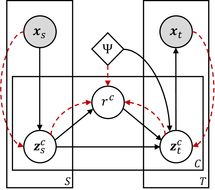
(a) The graphical model of RAISE

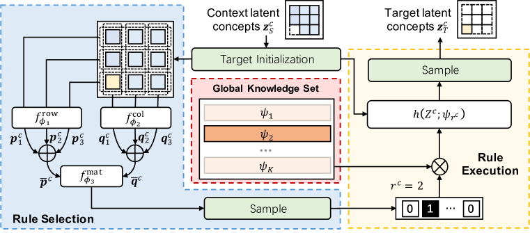
(b) The abstract reasoning process

Figure 1: An overview of RAISE. The graphical model in (a) displays the generative process (solid black lines) and inference process (dashed red lines). Panel (b) shows the computational details of the abstract reasoning process and highlights the rule selection, rule execution, and global knowledge with blue, yellow, and red backgrounds, respectively.

3.1 Conditional Generation

The generative process is the foundation of answer generation, including the stage of concept learning, abstract reasoning, and image generation.

Concept Learning. RAISE extracts interpretable image representations for abstract reasoning and image generation in the concept learning stage. Previous studies have emphasized the role of abstract object representations in the abstract reasoning of infants Kahneman et al. (1992); Gordon & Irwin (1996), which is similar to the idea of object-centric representation learners that decompose complex scenes into object representations Locatello et al. (2020). Both views reflect the compositionality of human cognition Lake et al. (2011). We can follow similar ideas to convert relatively complex images into simpler latent concepts, and further decompose the overall rules of RPMs into atomic rules shared on the latent concepts. RAISE realizes attribute-level compositionality by encoding attributes of images into $C$ independent latent concepts Wu et al. (2020); Shi et al. (2021; 2023). In the first step, RAISE encodes a context image $\bm{x}_{s}$ into context latent concepts $\bm{z}_{s}=\{\bm{z}_{s}^{c}\}_{c=1}^{C}$:

$$\bm{\mu}_{s}^{1:C} =g_{\theta}^{\text{enc}}\left(\bm{x}_{s}\right), \quad s\in S,$$ (1)

$$\bm{z}_{s}^{c} \sim\mathcal{N}\left(\bm{\mu}_{s}^{c},\sigma_{z}^{2}\bm{I}\right), \quad c=1,..,C,\quad s\in S.$$

The encoder $g_{\theta}^{\text{enc}}$ predicts only the means of context latent concepts, and the standard deviation $\sigma_{z}$ is controlled by a hyperparameter to keep training stability. $g_{\theta}^{\text{enc}}$ handles each context image independently, making it possible to extract latent concepts for any set of input images. The encoder does not consider any relationships between images to focus on concept learning.

Abstract Reasoning. As illustrated in Figure 1(b), RAISE predicts the target latent concepts $\bm{z}_{T}$ from context latent concepts $\bm{z}_{S}$ in the abstract reasoning stage, involving rule abstraction, rule selection, and rule execution. To abstract atomic rules and build the global knowledge set, RAISE adopts $K$ groups of global learnable parameters $\psi=\{\psi_{k}\}_{k=1}^{K}$, each indicating an atomic rule that can be shared among RPMs. In the process of rule selection, we use indicators $\{r^{c}\}_{c=1}^{C}$ ($r^{c}=1,...,K$) to select proper rules for each concept out of the global knowledge set $\psi$. The critical of rule selection is to infer the indicators based on $\bm{z}_{S}$. To this end, we first create a 3$\times$3 representation matrix $\bm{Z}^{c}$ for each concept through random target initialization. In the matrix, the representations of context images are filled with the corresponding context latent concepts while those of target images are initialized as zero vectors. Then RAISE extracts the representations for rows and columns:

$$\begin{gathered}\bm{p}_{i}^{c}=f_{\phi_{1}}^{\text{row}}\left(\bm{Z}^{c}_{i,1:3}\right),\quad\bm{q}_{i}^{c}=f_{\phi_{2}}^{\text{col}}\left(\bm{Z}^{c}_{1:3,i}\right),\quad i=1,2,3,\quad c=1,...,C.\end{gathered}$$ (2)

RAISE averages the row and column representations to obtain $\bm{\bar{p}}^{c}=(\bm{p}_{1}^{c}+\bm{p}_{2}^{c}+\bm{p}_{3}^{c})/3$ and $\bm{\bar{q}}^{c}=(\bm{q}_{1}^{c}+\bm{q}_{2}^{c}+\bm{q}_{3}^{c})/3$, which are respectively overall representations along the row and column. We concatenate $\bm{\bar{p}}^{c}$ and $\bm{\bar{q}}^{c}$ to acquire the probability of selecting rules out of the global knowledge set:

$$\begin{gathered}r^{c}\sim\text{Categorical}\left(\bm{\pi}_{1:K}^{c}\right),\quad\pi_{1}^{c},...,\pi_{K}^{c}=f_{\phi_{3}}^{\text{ind}}\big{(}\bm{\bar{p}}^{c},\bm{\bar{q}}^{c}\big{)},\quad c=1,...,C.\end{gathered}$$ (3)

We denote the learnable parameters as $\phi=\{\phi_{1},\phi_{2},\phi_{3}\}$ for convenience. In rule execution, RAISE selects and executes an atomic rule on each concept to predict the target latent concepts:

$$\bm{\mu}_{T}^{c} =h\left(\bm{Z}^{c};\psi_{r^{c}}\right), \quad c=1,...,C,$$ (4)

$$\bm{z}_{t}^{c} \sim\mathcal{N}\left(\bm{\mu}_{t}^{c},\sigma_{z}^{2}\bm{I}\right), \quad t\in T,\quad c=1,...,C.$$

For each concept, the parameter of $h$ is selected from $\psi$ by the indicator $r^{c}$. The neural network $h$ converts the initialized target representations in $\bm{Z}^{c}$ to the means of target latent concepts. Like the concept learning stage, the standard deviation of target latent concepts is controlled by $\sigma_{z}$. RAISE realizes $h$ with convolution layers to predict target latent concepts from the context via message passing on the matrix. Each group of parameters in $\psi$ is the learnable parameters of $h$ that indicate an atomic rule in the global knowledge set. See Appendix C.1 for the detailed description of $h$.

Image Generation. After obtaining target latent concepts in abstract reasoning, RAISE decodes the latent concepts into target images, which is

$$\begin{gathered}\bm{x}_{t}\sim\mathcal{N}\left(\bm{\Lambda}_{t},\sigma_{x}^{2}\bm{I}\right),\quad\bm{\Lambda}_{t}=g_{\varphi}^{\text{dec}}\left(\bm{z}_{t}^{1:C}\right),\quad t\in T.\end{gathered}$$ (5)

RAISE generates each target image independently to make the decoder focus on image reconstruction and controls the noise of target images by setting $\sigma_{x}$ as a hyperparameter.

According to Figure 1(a), we decompose the conditional generative process as

$$p_{\Theta}(\bm{h},\bm{x}_{T}|\bm{x}_{S})=\prod_{t\in T}p_{\varphi}(\bm{x}_{t}|\bm{z}_{t})\prod_{c=1}^{C}\left(p_{\psi}(\bm{z}_{T}^{c}|r^{c},\bm{z}_{S}^{c})p_{\phi}(r^{c}|\bm{z}_{S}^{c})\prod_{s\in S}p_{\theta}(\bm{z}_{s}^{c}|\bm{x}_{s})\right)$$ (6)

where $\bm{h}$ is the set of all latent variables and $\Theta=\{\theta,\phi,\psi,\varphi\}$ are learnable parameters of RAISE.

3.2 Variational Inference

RAISE approximates the untractable posterior with a variational distribution $q(\bm{h}|\bm{x}_{T},\bm{x}_{S})$ Kingma & Welling (2013), which consists of the following distributions.

$$q(\bm{z}_{s}^{c}|\bm{x}_{s}) =\mathcal{N}\left(\bm{\tilde{\mu}}_{s}^{c},\sigma_{z}^{2}\bm{I}\right), \quad s\in S,\quad c=1,...,C,$$ (7)

$$q(\bm{z}_{t}^{c}|\bm{x}_{t}) =\mathcal{N}\left(\bm{\tilde{\mu}}_{t}^{c},\sigma_{z}^{2}\bm{I}\right), \quad t\in T,\quad c=1,...,C,$$

$$q(r^{c}|\bm{z}_{S}^{c},\bm{z}_{T}^{c}) =\text{Categorical}\left(\bm{\tilde{\pi}}_{1:K}^{c}\right), c=1,...,C.$$

To reduce the model parameters, we share the encoder between the generative and inference processes. Therefore, $\bm{\tilde{\mu}}_{s}^{1:C}$ and $\bm{\tilde{\mu}}_{t}^{1:C}$ are computed via the same process described by Equation 1. In rule selection, RAISE reformulates the variational posterior of the indicator as $q(r^{c}|\bm{z}_{S}^{c},\bm{z}_{T}^{c})\propto p(\bm{z}_{T}^{c}|r^{c},\bm{z}_{S}^{c})p(r^{c}|\bm{z}_{S}^{c})$. We first predict the prior categorical probability $\bm{\pi}_{1:K}^{c}$ of $p(r^{c}|\bm{z}_{S}^{c})$ from the context $\bm{z}_{S}^{c}$. Then we predict the target concepts by executing each atomic rule on $\bm{z}_{S}^{c}$ and compute the likelihood $p(\bm{z}_{T}^{c}|r^{c},\bm{z}_{S}^{c})$ of each atomic rule. $q(r^{c}|\bm{z}_{S}^{c},\bm{z}_{T}^{c})$ is estimated by considering both the prior categorical probability and likelihood comprehensively, which reduces the risk of model collapse (e.g., the model always selects one rule). We provide the derivation of $q(r^{c}|\bm{z}_{S}^{c},\bm{z}_{T}^{c})$ in Appendix A.1. Letting $\Psi=\{\theta,\phi,\psi\}$, we factorize the variational distribution as

$$q_{\Psi}(\bm{h}|\bm{x}_{T},\bm{x}_{S})=\prod_{c=1}^{C}q_{\phi,\psi}(r^{c}|\bm{z}_{S}^{c},\bm{z}_{T}^{c})\prod_{s\in S}q_{\theta}(\bm{z}_{s}^{c}|\bm{x}_{s})\prod_{t\in T}q_{\theta}(\bm{z}_{t}^{c}|\bm{x}_{t}).$$ (8)

3.3 Parameter Learning

We update the parameters of RAISE by maximizing the evidence lower bound (ELBO) to approximately optimize the log-likelihood $\log p(\bm{x}_{T}|\bm{x}_{S})$ Kingma & Welling (2013). With the generative process $p_{\Theta}$ and the variational distribution $q_{\Psi}$ defined in Equations 6 and 8, the ELBO is

$$\mathcal{L} =\mathbb{E}_{q_{\Psi}(\bm{h}|\bm{x}_{T},\bm{x}_{S})}\left[\log\frac{p_{\Theta}\left(\bm{h},\bm{x}_{T}|\bm{x}_{S}\right)}{q_{\Psi}(\bm{h}|\bm{x}_{T},\bm{x}_{S})}\right]$$ (9)

$$=\underbrace{\sum_{t\in T}\mathbb{E}_{q}\big{[}\log p(\bm{x}_{t}|\bm{z}_{t})\big{]}}_{\text{$\mathcal{L}_{\text{rec}}$}}-\underbrace{\sum_{c=1}^{C}\mathbb{E}_{q}\left[\log\frac{\prod_{t\in T}q(\bm{z}_{t}^{c}|\bm{x}_{t})}{p(\bm{z}_{T}^{c}|r^{c},\bm{z}_{S}^{c})}\right]}_{\text{$\mathcal{R}_{\text{pred}}$}}-\underbrace{\sum_{c=1}^{C}\mathbb{E}_{q}\left[\log\frac{q(r^{c}|\bm{z}_{S}^{c},\bm{z}_{T}^{c})}{p(r^{c}|\bm{z}_{S}^{c})}\right]}_{\text{$\mathcal{R}_{\text{rule}}$}}$$

where $q$ denotes $q_{\Psi}(\bm{h}|\bm{x}_{T},\bm{x}_{S})$, and the parameter symbols are omitted for convenience. $\mathcal{L}_{\text{rec}}$ is reconstruction loss that measures the quality of the reconstruction images. The concept regularizer $\mathcal{R}_{\text{pred}}$ estimates the distance between the predicted target concepts and those directly encoded from target images. Minimizing $\mathcal{R}_{\text{pred}}$ will promote RAISE to generate correct predictions of latent concepts. The rule regularizer $\mathcal{R}_{\text{rule}}$ makes RAISE select the same rules when given different context images of a matrix. The variational posterior $q_{\phi,\psi}(r^{c}|\bm{z}_{S}^{c},\bm{z}_{T}^{c})$ conditioned on the entire matrix and the prior $p_{\phi}(r^{c}|\bm{z}_{S}^{c})$ conditioned on the context images are expected to have similar probabilities. The detailed derivation of the ELBO is provided in Appendix A.2.

As the rule abstraction and selection are based on concept learning, RAISE introduces auxiliary rule annotations to help stabilize the learning of latent concepts. A rule annotation $\bm{v}=\{v_{a}\}_{a=1}^{A}$ contains indicator variables of $A$ ground truth attributes to illustrate the rule on each attribute. For example, If there are three ground truth attributes, the rule annotation $\bm{v}=[1,0,2]$ where each element indicates the rule types on one attribute. In training, RAISE will not leverage the meta information of attributes. RAISE is informed of the rule types on three attributes, but does not know what the attributes represent. Therefore, we need to determine the correspondence between latent concepts and attributes, so that each ground truth indicator can guide the learning of related latent concepts. RAISE introduces a $A\times C$ binary matrix $\bm{M}$ where $\bm{M}_{a,c}=1$ means that the $a$th attribute is related to the $c$th concept. An auxiliary loss is used to measure the accuracy of rule selection:

$$\mathcal{L}_{\text{sup}}=\frac{1}{2}\sum_{a=1}^{A}\sum_{c=1}^{C}\bm{M}_{a,c}\log\left(\pi_{v_{a}}^{c}+\tilde{\pi}_{v_{a}}^{c}\right).$$ (10)

$\mathcal{L}_{\text{sup}}$ is the log-likelihood of the category distributions considering the attribute-concept correspondence $\bm{M}$. The binary matrix $\bm{M}$ is determined by solving

$$\begin{gathered}\operatorname*{arg\,max}_{\bm{M}}\mathcal{L}_{\text{sup}}\quad\text{s.t.}\quad\begin{cases}\sum_{c=1}^{C}\bm{M}_{a,c}=1,&a=1,...,A,\\ \sum_{a=1}^{A}\bm{M}_{a,c}=0\text{ or }1,&c=1,...,C,\\ \bm{M}_{a,c}=0\text{ or }1,&a=1,...,A,\quad c=1,...,C.\end{cases}\end{gathered}$$ (11)

The assignment problem can be solved by the modified Jonker-Volgenant algorithm Crouse (2016). Equation 11 handles the redundancy of concepts by allowing some latent concepts not to encode any attribute. Including the auxiliary loss, the training objective is

$$\operatorname*{arg\,max}_{\Theta}\mathcal{L}_{\text{rec}}-\beta_{1}\mathcal{R}_{\text{pred}}-\beta_{2}\mathcal{R}_{\text{rule}}+\beta_{3}\mathcal{L}_{\text{sup}}$$ (12)

where $\beta_{1}$, $\beta_{2}$, and $\beta_{3}$ are hyperparameters to control the importance of subterms. The training of RAISE supports semi-supervised settings. For samples that do not provide rule annotations, RAISE can set $\beta_{3}=0$ and update parameters via the unsupervised part $\mathcal{L}_{\text{rec}}-\beta_{1}\mathcal{R}_{\text{pred}}-\beta_{2}\mathcal{R}_{\text{rule}}$.

4 Experiments

In the experiments, we compare the performance of RAISE with other generative solvers by generating answers at the bottom right and, more challenging, arbitrary positions. Then we conduct experiments to visualize the latent concepts learned from the dataset. Finally, RAISE carries out the odd-one-out task and is tested in held-out configurations to illustrate the benefit of learning latent concepts and atomic rules in generative abstract reasoning.

Datasets. The models in the experiments are evaluated on the RAVEN Zhang et al. (2019a) and I-RAVEN Hu et al. (2021) datasets having seven image configurations (e.g., scenes with centric objects or object grids) and four basic rules. I-RAVEN follows the same configurations as RAVEN and reduces the bias of candidate sets to resist the shortcut learning of models Hu et al. (2021). See Appendix B for detailed descriptions of datasets.

Compared Models. In the bottom-right answer selection task, we compare RAISE with the powerful generative solvers ALANS Zhang et al. (2021b), PrAE Zhang et al. (2021a), and the model proposed by Niv et al. (called GCA for convenience) Pekar et al. (2020). RAISE selects the candidate closest to the predicted result in the latent space as the answer. We apply three strategies of answer selection in GCA: selecting the candidate having the smallest pixel difference to the prediction (GCA-I), having the smallest difference in the representation space (GCA-R), and having the highest panel score (GCA-C). Since these generative solvers cannot generate non-bottom-right answers, we take Transformer Vaswani et al. (2017), ANP Kim et al. (2019), LGPP Shi et al. (2021), and CLAP Shi et al. (2023) as baseline models to evaluate the ability to generate answers at arbitrary positions. We give more detail about the related models in Appendix C.

Training and Evaluation Settings. For non-grid layouts, RAISE is trained under semi-supervised settings by using 5% rule annotations. RAISE leverages 20% rule annotations on O-IG and full rule annotations on 2$\times$2Grid and 3$\times$3Grid. The powerful generative solvers use full rule annotations and are trained and tested on each configuration respectively. We compare RAISE with them to illustrate the acquired bottom-right answer selection ability of RAISE under semi-supervised settings. The baselines can generate answers at arbitrary positions but cannot leverage rule annotations since they do not explicitly model the category of rules. We compare RAISE with the baselines to illustrate the benefit of learning latent concepts and atomic rules for generative abstract reasoning. Since the training of RAISE and the baselines do not require the candidate sets, and RAVEN/I-RAVEN only differ in the distribution of candidates, we train RAISE and the baselines on RAVEN and test them on both RAVEN/I-RAVEN directly. See Appendix C for detailed training and evaluation settings.

4.1 Bottom-Right Answer Selection

Table 1: The accuracy (%) of selecting bottom-right answers on RAVEN/I-RAVEN. For models with randomness, the table displays the average results of ten trials.

Models	Average	Center	L-R	U-D	O-IC	O-IG	2$\times$2Grid	3$\times$3Grid
GCA-I	12.0/24.1	14.0/30.2	7.9/22.4	7.5/26.9	13.4/32.9	15.5/25.0	11.3/16.3	14.5/15.3
GCA-R	13.8/27.4	16.6/34.5	9.4/26.9	6.9/28.0	17.3/37.8	16.7/26.0	11.7/19.2	18.1/19.3
GCA-C	32.7/41.7	37.3/51.8	26.4/44.6	21.5/42.6	30.2/46.7	33.0/35.6	37.6/38.1	43.0/32.4
ALANS	54.3/62.8	42.7/63.9	42.4/60.9	46.2/65.6	49.5/64.8	53.6/52.0	70.5/66.4	75.1/65.7
PrAE	80.0/85.7	97.3/99.9	96.2/97.9	96.7/97.7	95.8/98.4	68.6/76.5	82.0/84.5	23.2/45.1
LGPP	6.4/16.3	9.2/20.1	4.7/18.9	5.2/21.2	4.0/13.9	3.1/12.3	8.6/13.7	10.4/13.9
ANP	7.3/27.6	9.8/47.4	4.1/20.3	3.5/20.7	5.4/38.2	7.6/36.1	10.0/15.0	10.5/15.6
CLAP	17.5/32.8	30.4/42.9	13.4/35.1	12.2/32.1	16.4/37.5	9.5/26.0	16.0/20.1	24.3/35.8
Transformer	40.1/64.0	98.4/99.2	67.0/91.1	60.9/86.6	14.5/69.9	13.5/57.1	14.7/25.2	11.6/18.6
RAISE	90.0/92.1	99.2/99.8	98.5/99.6	99.3/99.9	97.6/99.6	89.3/96.0	68.2/71.3	77.7/78.7

A classic RPM test requires participants to select an answer from the candidate set to fill in the missing image at the bottom right. The results in Table 1 illustrate RAISE’s outstanding generative abstract reasoning ability. By comparing the difference between predictions and candidates, RAISE outperforms the compared generative solvers in most configurations of RAVEN and I-RAVEN, even if the distractors in candidate sets are not used in training. All the powerful generative solvers take full rule annotations for training, while RAISE in non-grid configurations only requires a small amount of rule annotations (5% samples) to achieve high selection accuracy. RAISE attains the highest selection accuracy compared to the baselines which can generate answers at arbitrary positions. By comparing the results on RAVEN and I-RAVEN, we find that the generative solvers are more likely to have accuracy improvement on I-RAVEN. I-RAVEN generates distractors less similar to correct answers than RAVEN to avoid significant biases in candidate sets, making answer selection easier. For grid-shaped configurations, we found that the noise in datasets will significantly influence the model performance. By removing the noise in object attributes, RAISE achieves high selection accuracy on three grid-shaped configurations using only 20% rule annotations. See Appendix D.1 for the detailed descriptions and experimental results.

4.2 Answer Selection at Arbitrary Position

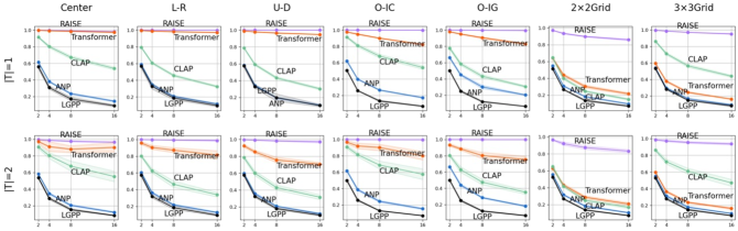
Figure 2: Selection accuracy at arbitrary positions. The selection accuracy of RAISE (purple), Transformer (orange), CLAP (green), ANP (blue), and LGPP (black) in arbitrary positions. The x-axis of each plot indicates the number of candidates, and the y-axis is the selection accuracy.

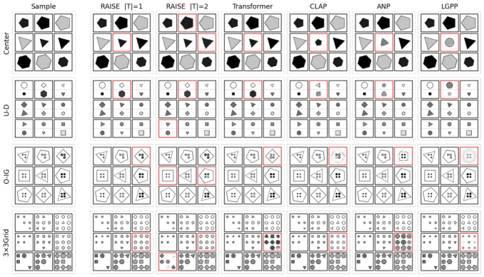
Figure 3: Answer generation at arbitrary positions. We give the predictions on RAVEN with red boxes to illustrate the ability of arbitrary-position answer generation. Some predictions of RAISE differ from the original sample, but they still follow the correct rules due to the existence of noise.

The above generative solvers can hardly generate answers at non-bottom-right positions. In this experiment, we probe the ability of RAISE and baselines to generate answers at arbitrary positions, which is acquired by predicting random target images in RPMs. We first generate additional candidate sets in the experiment because RAVEN and I-RAVEN do not provide candidate sets for non-bottom-right images. To this end, we sample a batch of RPMs from the dataset and split the RPMs into target and context images in the same way. For each matrix, we use the target images of other $N_{c}$ samples in the batch as distractors to generate a candidate set with $N_{c}+1$ entries. This strategy can adapt to the missing images at arbitrary and even multiple positions, and we can easily control the difficulty of answer selection through the number of distractors

Figure 2 displays the accuracy of RAISE and baselines when generating answers at arbitrary and multiple positions. RAISE maintains high accuracy in all configurations. Although Transformer has higher accuracy than the other three baselines, especially in non-grid scenes, the prediction accuracy drops significantly on 2$\times$2Grid and 3$\times$3Grid. Figure 3 provides the qualitative prediction results on RAVEN. It is difficult for ANP and LGPP to generate clear answers. CLAP can generate answers with partially correct attributes in simple cases (e.g., CLAP generates an object with the correct color but the wrong size and shape in the sample of Center). RAISE produces high-quality predictions and can solve RPMs with multiple missing images. By predicting multiple missing images at arbitrary positions, The qualitative results intuitively reveal the in-depth generative abstract reasoning ability in models, which the bottom-right answer generation task does not involve.

4.3 Latent Concepts

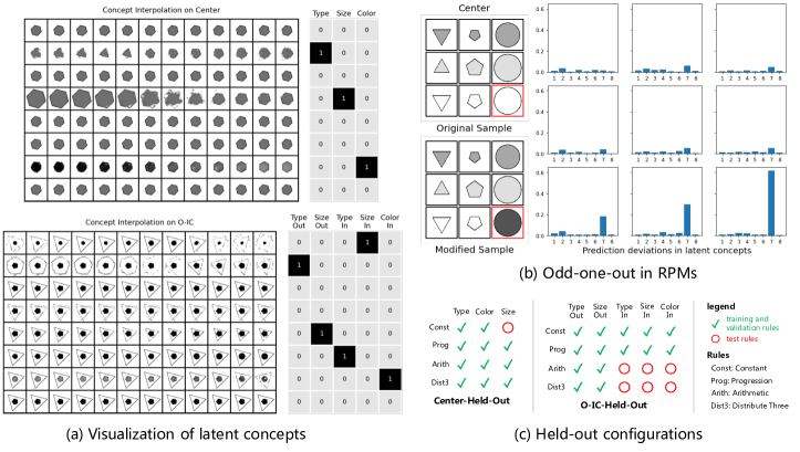
Figure 4: Panel (a) shows the interpolation results of latent concepts and the correspondence between the concepts and attributes. Panel (b) provides an example of RPM-based odd-one-out tests and displays the prediction deviations in concepts of each image. Panel (c) illustrates the strategy to split rule-attribute combinations in held-out configurations.

Latent concepts bridge atomic rules and high-dimensional observations. Figure 4a visualizes the latent concepts learned from Center and O-IC by traversing concept representations of an image in the latent space. If the concepts are well decomposed, decoding the interpolated concept representations will change one attribute of the original image. Besides observing visualization results, we can find the correspondence between concepts and attributes with the aid of the binary matrix $\bm{M}$. As shown in Figure 4a, RAISE can automatically set some redundant concepts when there are more concepts than attributes. (e.g., the 1st, 3rd, 5th, 6th, and 8th concepts of the configuration Center). The visualization results illustrate the concept learning ability of RAISE, which is the foundation of abstracting and selecting global atomic rules shared among RPMs.

4.4 Odd-One-Out in RPM

In odd-one-out tests, RAISE attempts to pick up the image that breaks the underlying rule of a panel. To generate RPM-based odd-one-out problems, we replace the bottom-right image of an RPM with a random distractor in the candidate set. Taking Figure 4b as an example, by replacing the bottom-right image, we change the object color from white to black. RAISE takes each image in the RPM as the target, gets the prediction results, and computes the distance in concepts between the predictions and original images. The right panel of Figure 4b shows the concept distances of each image, and we find that the 7th concept of the bottom-right image deviates the most. According to Figure 4a, the 5th concept on Center represents the attribute Color (i.e., the type of inner object), which is indeed the attribute modified when constructing the test. The last row has relatively higher concept distances since the incorrect image tends to influence the accuracy of answer generation at the most related positions. However, because the concepts and concept-specific rules are designed as independent in RAISE, the high concept distances only appear in the 7th concept. By solving RPM-based odd-one-out problems in this experiment, we explain how concept-level predictions improve the interpretability of answer selection. Though RAISE is tasked with generating answers, it can handle answer-selection problems by excluding candidates that violate the underlying rules.

4.5 Held-Out Configurations

Table 2: Selection accuracy (%) on two held-out configurations.

OOD Settings	RAISE	PrAE	ALANS	GCA-C	GCA-R	GCA-I	Transformer	ANP	LGPP	CLAP-NP
Center-Held-Out	99.2	99.8	46.9	35.0	14.4	12.1	12.1	10.6	8.6	19.5
O-IC-Held-Out	56.1	40.5	33.4	10.1	5.3	4.9	15.8	7.5	4.6	8.6

To explore the abstract reasoning ability on out-of-distribution (OOD) samples, we construct two held-out configurations based on RAVEN Barrett et al. (2018) as illustrated in Figure 4c. (1) Center-Held-Out keeps the samples of Center following the attribute-rule tuple (Size, Constant) as test samples, and the remaining constitute the training and validation sets. (2) O-IC-Held-Out keeps the samples of O-IC following the attribute-rule tuples (Type In, Arithmetic), (Size In, Arithmetic), (Color In, Arithmetic), (Type In, Distribute Three), (Size In, Distribute Three), and (Color In, Distribute Three) as test samples. The results given in Table 2 indicate that RAISE maintains relatively higher selection accuracy when encountering unseen combinations of attributes and rules. RAISE learns interpretable latent concepts to conduct concept-specific reasoning, by which the learning of rules and concepts are decoupled. Thus RAISE can tackle OOD samples via compositional generalization. Although RAISE has not ever seen the attribute-rule tuple (Size, Constant) in training, it can still apply the atomic rule Constant learned from other attributes to Size in the test phase.

5 Conclusion and Discussion

This paper proposes a generative RPM solver RAISE based on conditional deep latent variable models. RAISE can abstract atomic rules from PRMs, keep them in the global knowledge set, and predict target images by selecting proper rules. As the foundation of rule abstraction and selection, RAISE learns interpretable latent concepts from images to decompose the integrated rules of RPMs into atomic rules. Qualitative and quantitative experiments show that RAISE can generate answers at arbitrary positions and outperform baselines, showing outstanding generative abstract reasoning. The odd-one-out task and held-out configurations verify the interpretability of RAISE in concept learning and rule abstraction. By using prediction deviations on concepts, RAISE can find the position and concept that breaks the rules in odd-one-out tasks. By combining the learned latent concepts and atomic rules, RAISE can generate answers on samples with unseen attribute-rule tuples.

Limitations and Discussion. The noise in data is a challenge for the models based on conditional generation. In the experiment, we find the noise of object attributes in grids will influence the selection accuracy of generative solvers like RAISE and Transformer on 2$\times$2Grid. The candidate sets can provide clearer supervision in training to reduce the impact of noise. Deep latent variable models (DLVMs) can potentially handle noise in RPMs since RAISE works well in Center and O-IC with noisy attributes like Rotation. In future works, exploring appropriate ways to reduce the influence of noise is the key to realizing generative abstract reasoning in more complicated scenes. However, for generative solvers that do not rely on candidate sets or are completely unsupervised, the noise level of datasets is a problem worth discussing. Too much noise will make a problem have a large number of solutions (e.g., PGM Barrett et al. (2018)), such data may not be proper for validating the generative reasoning ability of models. In Appendices B.2 and D.1, we conduct an initial experiment and discussion on the impact of noise, but a more systematic and in-depth study will be carried out in the follow-up works.

Appendix A Proofs and Derivations

A.1 Reformulation of the posterior distribution

The posterior distribution $q(r^{c}|\bm{z}_{S}^{c},\bm{z}_{T}^{c})$ can be computed from the prior $q(r^{c}|\bm{z}_{S}^{c})$ and the likelihood $p(\bm{z}_{T}^{c}|r^{c},\bm{z}_{S}^{c})$ in Bayes’ theorem:

$$q(r^{c}|\bm{z}_{S}^{c},\bm{z}_{T}^{c})=\frac{p(\bm{z}_{T}^{c}|r^{c},\bm{z}_{S}^{c})p(r^{c}|\bm{z}_{S}^{c})}{\sum_{k=1}^{K}p(\bm{z}_{T}^{c}|r^{c}=k,\bm{z}_{S}^{c})p(r^{c}=k|\bm{z}_{S}^{c})}\propto p(\bm{z}_{T}^{c}|r^{c},\bm{z}_{S}^{c})p(r^{c}|\bm{z}_{S}^{c}).$$ (13)

According to Equation 4, $p(\bm{z}_{T}^{c}|r^{c},\bm{z}_{S}^{c})$ is a Gaussian distribution with the mean $h\left(\bm{Z}^{c};\psi_{r^{c}}\right)$ and the standard deviation $\sigma_{z}$. Therefore, Equation 13 can be expressed as

$$q(r^{c}|\bm{z}_{S}^{c},\bm{z}_{T}^{c}) \propto\frac{1}{\sqrt{2\pi\sigma_{z}^{\text{D}(\bm{z}_{T}^{c})}}}\exp\left(-\frac{1}{2\sigma^{2}_{z}}\Big{\|}\bm{z}_{T}^{c}-h\left(\bm{Z}^{c};\psi_{r^{c}}\right)\Big{\|}_{2}^{2}\right)p(r^{c}|\bm{z}_{S}^{c})$$ (14)

$$\propto\exp\left(-\frac{1}{2\sigma^{2}_{z}}\Big{\|}\bm{z}_{T}^{c}-h\left(\bm{Z}^{c};\psi_{r^{c}}\right)\Big{\|}_{2}^{2}\right)p(r^{c}|\bm{z}_{S}^{c}),$$

where $\text{D}(\bm{z}_{T}^{c})$ is the size of $\bm{z}_{T}^{c}$. In practice, neural networks output unnormalized logits $\bm{\tilde{l}}_{1:K}^{c}$ instead of the probabilities $\bm{\tilde{\pi}}_{1:K}^{c}$. Therefore, we use the logarithmic version of Equation 14:

$$\begin{gathered}\log q(r^{c}|\bm{z}_{S}^{c},\bm{z}_{T}^{c})=-\frac{1}{2\sigma_{z}^{2}}\Big{\|}\bm{z}_{T}^{c}-h\left(\bm{Z}^{c};\Psi_{r^{c}}\right)\Big{\|}_{2}^{2}+\log p(r^{c}|\bm{z}_{S}^{c})+C\left(\bm{z}_{S}^{c},\bm{z}_{T}^{c}\right).\\ \end{gathered}$$ (15)

$C(\bm{z}_{S}^{c},\bm{z}_{T}^{c})$ is not related to $r^{c}$ and thus will not influence the results of the softmax operation on $r^{c}$. RAISE ignores $C(\bm{z}_{S}^{c},\bm{z}_{T}^{c})$ in Equation 15 and predicts the unnormalized logits via

$$\tilde{l}_{k}^{c} =-\frac{1}{2\sigma^{2}_{z}}\Big{\|}\bm{z}_{T}^{c}-h\left(\bm{Z}^{c};\Psi_{k}\right)\Big{\|}_{2}^{2}+\log p(r^{c}=k|\bm{z}_{S}^{c})$$ (16)

$$=-\frac{1}{2\sigma^{2}_{z}}\Big{\|}\bm{z}_{T}^{c}-h\left(\bm{Z}^{c};\Psi_{k}\right)\Big{\|}_{2}^{2}+\log\pi_{k}^{c},\quad k=1,...,K.$$

Finally, the variational distribution $q(r^{c}|\bm{z}_{S}^{c},\bm{z}_{T}^{c})$ is parameterized by

$$q(r^{c}|\bm{z}_{S}^{c},\bm{z}_{T}^{c}) =\text{Categorical}\left(\bm{\tilde{\pi}}_{1:K}^{c}\right),\quad\text{where }\tilde{\pi}_{k}^{c}=\frac{\exp\left(\tilde{l}_{k}^{c}\right)}{\sum_{k=1}^{K}\exp\left(\tilde{l}_{k}^{c}\right)}\text{ for }k=1,...,K.$$ (17)

A.2 Derivation of the ELBO

With the variational distribution $q_{\Psi}(\bm{h}|\bm{x}_{T},\bm{x}_{S})$, the ELBO $\mathcal{L}$ is []sohn2015learning

$$\begin{gathered}\log p_{\Theta}\left(\bm{x}_{T}|\bm{x}_{S}\right)\geq\mathbb{E}_{q_{\Psi}(\bm{h}|\bm{x}_{T},\bm{x}_{S})}\left[\log\frac{p_{\Theta}\left(\bm{h},\bm{x}_{T}|\bm{x}_{S}\right)}{q_{\Psi}(\bm{h}|\bm{x}_{T},\bm{x}_{S})}\right]=\mathcal{L}.\end{gathered}$$ (18)

Considering the generative process and inference processes

$$p_{\Theta}(\bm{h},\bm{x}_{T}|\bm{x}_{S}) =\prod_{t\in T}p_{\varphi}(\bm{x}_{t}|\bm{z}_{t})\prod_{c=1}^{C}\left(p_{\psi}(\bm{z}_{T}^{c}|r^{c},\bm{z}_{S}^{c})p_{\phi}(r^{c}|\bm{z}_{S}^{c})\prod_{s\in S}p_{\theta}(\bm{z}_{s}^{c}|\bm{x}_{s})\right),$$ (19)

$$q_{\Psi}(\bm{h}|\bm{x}_{T},\bm{x}_{S}) =\prod_{c=1}^{C}q_{\phi,\psi}(r^{c}|\bm{z}_{S}^{c},\bm{z}_{T}^{c})\prod_{s\in S}q_{\theta}(\bm{z}_{s}^{c}|\bm{x}_{s})\prod_{t\in T}q_{\theta}(\bm{z}_{t}^{c}|\bm{x}_{t}),$$

Equation 18 is further decomposed by

$$\mathcal{L} =\mathbb{E}_{q_{\Psi}(\bm{h}|\bm{x}_{T},\bm{x}_{S})}\left[\log\prod_{t\in T}p_{\varphi}(\bm{x}_{t}|\bm{z}_{t})\right]$$ (20)

$$\quad-\mathbb{E}_{q_{\Psi}(\bm{h}|\bm{x}_{T},\bm{x}_{S})}\left[\log\prod_{c=1}^{C}\frac{q_{\phi,\psi}(r^{c}|\bm{z}_{S}^{c},\bm{z}_{T}^{c})\prod_{s\in S}q_{\theta}(\bm{z}_{s}^{c}|\bm{x}_{s})\prod_{t\in T}q_{\theta}(\bm{z}_{t}^{c}|\bm{x}_{t})}{p_{\psi}(\bm{z}_{T}^{c}|r^{c},\bm{z}_{S}^{c})p_{\phi}(r^{c}|\bm{z}_{S}^{c})\prod_{s\in S}p_{\theta}(\bm{z}_{s}^{c}|\bm{x}_{s})}\right]$$

$$=\sum_{t\in T}\mathbb{E}_{q_{\Psi}(\bm{h}|\bm{x}_{T},\bm{x}_{S})}\big{[}\log p_{\varphi}(\bm{x}_{t}|\bm{z}_{t})\big{]}-\sum_{c=1}^{C}\mathbb{E}_{q_{\Psi}(\bm{h}|\bm{x}_{T},\bm{x}_{S})}\left[\log\frac{\prod_{t\in T}q_{\theta}(\bm{z}_{t}^{c}|\bm{x}_{t})}{p_{\psi}(\bm{z}_{T}^{c}|r^{c},\bm{z}_{S}^{c})}\right]$$

$$\quad-\sum_{c=1}^{C}\mathbb{E}_{q_{\Psi}(\bm{h}|\bm{x}_{T},\bm{x}_{S})}\left[\log\frac{q_{\phi,\psi}(r^{c}|\bm{z}_{S}^{c},\bm{z}_{T}^{c})}{p_{\phi}(r^{c}|\bm{z}_{S}^{c})}\right]-\sum_{c=1}^{C}\sum_{s\in S}\mathbb{E}_{q_{\Psi}(\bm{h}|\bm{x}_{T},\bm{x}_{S})}\left[\log\frac{q_{\theta}(\bm{z}_{s}^{c}|\bm{x}_{s})}{p_{\theta}(\bm{z}_{s}^{c}|\bm{x}_{s})}\right].$$

Since the encoder is shared between the generative and inference processes, we have $q_{\theta}(\bm{z}_{s}^{c}|\bm{x}_{s})=p_{\theta}(\bm{z}_{s}^{c}|\bm{x}_{s})$ and then

$$\sum_{c=1}^{C}\sum_{s\in S}\mathbb{E}_{q_{\Psi}(\bm{h}|\bm{x}_{T},\bm{x}_{S})}\left[\log\frac{q_{\theta}(\bm{z}_{s}^{c}|\bm{x}_{s})}{p_{\theta}(\bm{z}_{s}^{c}|\bm{x}_{s})}\right]=0.$$ (21)

Therefore, the ELBO is

$$\mathcal{L} =\underbrace{\sum_{t\in T}\mathbb{E}_{q_{\Psi}(\bm{h}|\bm{x}_{T},\bm{x}_{S})}\big{[}\log p_{\varphi}(\bm{x}_{t}|\bm{z}_{t})\big{]}}_{\text{$\mathcal{L}_{\text{rec}}$}}-\underbrace{\sum_{c=1}^{C}\mathbb{E}_{q_{\Psi}(\bm{h}|\bm{x}_{T},\bm{x}_{S})}\left[\log\frac{\prod_{t\in T}q_{\theta}(\bm{z}_{t}^{c}|\bm{x}_{t})}{p_{\psi}(\bm{z}_{T}^{c}|r^{c},\bm{z}_{S}^{c})}\right]}_{\text{$\mathcal{R}_{\text{pred}}$}}$$ (22)

$$\quad\quad-\underbrace{\sum_{c=1}^{C}\mathbb{E}_{q_{\Psi}(\bm{h}|\bm{x}_{T},\bm{x}_{S})}\left[\log\frac{q_{\phi,\psi}(r^{c}|\bm{z}_{S}^{c},\bm{z}_{T}^{c})}{p_{\phi}(r^{c}|\bm{z}_{S}^{c})}\right]}_{\text{$\mathcal{R}_{\text{rule}}$}}.$$

A.3 Monte Carlo Estimator of the ELBO

To compute $\mathcal{L}$ for a given RPM $(\bm{x}_{S},\bm{x}_{T})$, we sample the latent variables $\bm{\tilde{r}}$, $\bm{\tilde{z}}_{S}$, and $\bm{\tilde{z}}_{T}$ from the variatonal posterior $q_{\Psi}(\bm{h}|\bm{x}_{T},\bm{x}_{S})$ through

$$\bm{\tilde{z}}_{s}^{c} \sim\mathcal{N}\left(\bm{\tilde{\mu}}_{s}^{c},\sigma_{z}^{2}\bm{I}\right), \quad s\in S,\quad c=1,...,C,$$ (23)

$$\bm{\tilde{z}}_{t}^{c} \sim\mathcal{N}\left(\bm{\tilde{\mu}}_{t}^{c},\sigma_{z}^{2}\bm{I}\right), \quad t\in T,\quad c=1,...,C,$$

$$\tilde{r}^{c} \sim\text{Categorical}\left(\bm{\tilde{\pi}}_{1:K}^{c}\right), c=1,...,C.$$

$\bm{\tilde{\mu}}_{s}^{1:C}=g_{\theta}^{\text{enc}}(\bm{x}_{s})$ and $\bm{\tilde{\mu}}_{t}^{1:C}=g_{\theta}^{\text{enc}}(\bm{x}_{t})$ are means of latent concepts computed by the encoder. $\bm{\tilde{\pi}}_{1:K}^{c}$ is given by 17 and the indicator $\tilde{r}^{c}$ is sampled through the Gumbel-Softmax distribution []jang2016categorical. Using the Monte Carlo estimator, $\mathcal{L}$ can be approximated by the samples of the posterior.

A.3.1 Reconstruction Loss

$$\mathcal{L}_{\text{rec}}\approx\sum_{t\in T}\log p_{\varphi}(\bm{x}_{t}|\bm{\tilde{z}}_{t})=-\frac{1}{2\sigma_{x}^{2}}\sum_{t\in T}\Big{\|}\bm{x}_{t}-\bm{\tilde{\Lambda}}_{t}\Big{\|}_{2}^{2}+C_{\text{rec}},\quad\text{where }\bm{\tilde{\Lambda}}_{t}=g_{\varphi}^{\text{dec}}(\bm{\tilde{z}}_{t}^{1:C})$$ (24)

A.3.2 Concept Regularizer

$$\mathcal{R}_{\text{pred}} =\sum_{c=1}^{C}\mathbb{E}_{q_{\theta}(\bm{z}_{T}^{c}|\bm{x}_{T})}\left[\mathbb{E}_{q_{\theta}(\bm{z}_{S}^{c}|\bm{x}_{S})}\left[\mathbb{E}_{q_{\phi,\psi}(r^{c}|\bm{\tilde{z}}_{S}^{c},\bm{\tilde{z}}_{T}^{c})}\left[\log\frac{\prod_{t\in T}q_{\theta}(\bm{z}_{t}^{c}|\bm{x}_{t})}{p_{\psi}(\bm{z}_{T}^{c}|r^{c},\bm{z}_{S}^{c})}\right]\right]\right]$$ (25)

$$\approx\sum_{c=1}^{C}\mathbb{E}_{q_{\theta}(\bm{z}_{S}^{c}|\bm{x}_{S})}\left[\mathbb{E}_{p_{\star}(r^{c}|\bm{x})}\left[\mathbb{E}_{q_{\theta}(\bm{z}_{T}^{c}|\bm{x}_{T})}\left[\log\frac{q_{\theta}(\bm{z}_{T}^{c}|\bm{x}_{T})}{p_{\psi}(\bm{z}_{T}^{c}|r^{c},\bm{z}_{S}^{c})}\right]\right]\right]$$

$$=\sum_{c=1}^{C}\mathbb{E}_{q_{\theta}(\bm{z}_{S}^{c}|\bm{x}_{S})}\Big{[}\mathbb{E}_{p_{\star}(r^{c}|\bm{x})}\big{[}D_{\text{KL}}\left(q_{\theta}(\bm{z}_{T}^{c}|\bm{x}_{T})||p_{\psi}(\bm{z}_{T}^{c}|r^{c},\bm{z}_{S}^{c})\right)\big{]}\Big{]}$$

$$\approx\sum_{c=1}^{C}D_{\text{KL}}\left(q_{\theta}(\bm{z}_{T}^{c}|\bm{x}_{T})\big{\|}p_{\psi}(\bm{z}_{T}^{c}|\tilde{r}^{c},\bm{\tilde{z}}_{S}^{c})\right)=\frac{1}{2\sigma_{z}^{2}}\sum_{c=1}^{C}\Big{\|}\bm{\tilde{\mu}}_{T}^{c}-\bm{\mu}_{T}^{c}\Big{\|}_{2}^{2}+C_{\text{pred}}.$$

Based on the supervision of $r^{c}$, RAISE can quickly approach the real distribution $p_{\star}(r^{c}|\bm{x})$ after the early learning stage. That is, the predicted rule distribution is close to the real one provided as the supervision, which is related to the image matrix itself rather than conditional on the latent concepts. Therefore, we assume that there is $q_{\phi,\psi}(r^{c}|\bm{\tilde{z}}_{S}^{c},\bm{\tilde{z}}_{T}^{c})\approx p_{\star}(r^{c}|\bm{x})$ after a few learning epochs, by which we can move the inner expectation on $r^{c}$ to the front. In this way, the inner expectation becomes the KL divergence between Gaussian distributions with a closed-form solution, which reduces the noise in the sampling process.

A.3.3 Rule Regularizer

$$\mathcal{R}_{\text{rule}} =\sum_{c=1}^{C}\mathbb{E}_{q_{\theta}(\bm{z}_{T}^{c}|\bm{x}_{T})}\left[\mathbb{E}_{q_{\theta}(\bm{z}_{S}^{c}|\bm{x}_{S})}\left[\mathbb{E}_{q_{\phi,\psi}(r^{c}|\bm{\tilde{z}}_{S}^{c},\bm{\tilde{z}}_{T}^{c})}\left[\log\frac{q_{\phi,\psi}(r^{c}|\bm{z}_{S}^{c},\bm{z}_{T}^{c})}{p_{\phi}(r^{c}|\bm{z}_{S}^{c})}\right]\right]\right]$$ (26)

$$=\sum_{c=1}^{C}\mathbb{E}_{q_{\theta}(\bm{z}_{T}^{c}|\bm{x}_{T})}\left[\mathbb{E}_{q_{\theta}(\bm{z}_{S}^{c}|\bm{x}_{S})}\left[D_{\text{KL}}\left(q_{\phi,\psi}(r^{c}|\bm{z}_{S}^{c},\bm{z}_{T}^{c})\big{\|}p_{\phi}(r^{c}|\bm{z}_{S}^{c})\right)\right]\right]$$

$$\approx\sum_{c=1}^{C}D_{\text{KL}}\left(q_{\phi,\psi}(r^{c}|\bm{\tilde{z}}_{S}^{c},\bm{\tilde{z}}_{T}^{c})\big{\|}p_{\phi}(r^{c}|\bm{\tilde{z}}_{S}^{c})\right)=\sum_{c=1}^{C}\sum_{k=1}^{K}\tilde{\pi}_{k}^{c}\log\frac{\tilde{\pi}_{k}^{c}}{\pi_{k}^{c}}.$$

A.3.4 ELBO

Ignoring the constants $C_{\text{rec}}$ and $C_{\text{pred}}$, the approximation of ELBO is

$$\mathcal{L}\approx\underbrace{-\frac{1}{2\sigma_{x}^{2}}\sum_{t\in T}\Big{\|}\bm{x}_{t}-\bm{\tilde{\Lambda}}_{t}\Big{\|}_{2}^{2}}_{\text{$\mathcal{L}_{\text{rec}}$}}-\underbrace{\frac{1}{2\sigma_{z}^{2}}\sum_{c=1}^{C}\Big{\|}\bm{\tilde{\mu}}_{T}^{c}-\bm{\mu}_{T}^{c}\Big{\|}_{2}^{2}}_{\text{$\mathcal{R}_{\text{pred}}$}}-\underbrace{\sum_{c=1}^{C}\sum_{k=1}^{K}\tilde{\pi}_{k}^{c}\log\frac{\tilde{\pi}_{k}^{c}}{\pi_{k}^{c}}}_{\text{$\mathcal{R}_{\text{rule}}$}}.$$ (27)

Appendix B Datasets

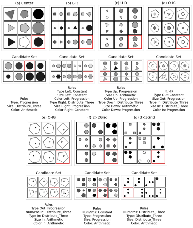
Figure 5: Samples from the seven image configurations of RAVEN. In (a)-(g), the top panels are 3$\times$3 RPMs where the target images are highlighted in red boxes; the middle panels are candidate sets; and the bottom panels show attribute-specific rules in the RPMs.

B.1 RAVEN and I-RAVEN

Figure 5 displays the seven image configurations of RAVEN []zhang2019raven. The attributes of an image can be Number/Position, Type, Size, and Color, which will change with the rules Constant, Progress, Arithmetic, and Distribution Three. In detail, these attribute-specific rules are:

1. Constant: an attribute stays unchanged in rows;

2. Progress: an attribute increases or decreases equidistantly in rows;

3. Arithmetic: the attribute of the third image is equal to the sum or difference of that in the first two images;

4. Distribution Three: the attribute in rows are three fixed values in different orders.

Each configuration contains 6000 training samples, 2000 validation samples, and 2000 test samples. RAVEN provides eight candidate images and attribute-level annotations of rules for RPMs.

RAVEN has biases in candidate generation []hu2021stratified, allowing models to find shortcuts in problem-solving. That is, the models trained with only candidate sets can achieve good selection accuracy. I-RAVEN uses Attribute Bisection Tree (ABT) to generate candidate sets to resist shortcut learning []hu2021stratified. The experiment shows that the models trained with only the candidate sets of I-RAVEN have a selection accuracy close to the random guesses, which evidences the effectiveness of the candidate generation strategy.

B.2 Attribute Noise of RAVEN and I-RAVEN

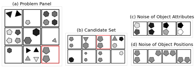
Figure 6: The illustration of attribute noise. (a) is an RPM from 2$\times$2Grid; (b) is the candidate set; (c) and (d) display two possible types of noise in the RPM. In this case, the image is correct as long as there are two pentagons of the correct size. The color, rotation, and position of objects will not influence the correctness of the image.

RAVEN and I-RAVEN introduce noise to some attributes to increase the complexity of problems. In Center, L-R, U-D, and O-IC, the rotation of objects is the noise attribute. That is, we can keep the rotation of objects constant in rows or randomly sample the rotations. Object grids in O-IG, 2$\times$2Grid, and 3$\times$3Grid have more complex noise. Figure 6 displays the noise of object grids, including the noise of object attributes (i.e., objects in Figure 6c can have different colors and rotations), and the noise of object positions (Figure 6d). The candidate set ensures that only one candidate image is the correct answer, which can provide clear supervision of the rule. To explore the influence of noise, we remove the noise of object attributes from O-IG, 2$\times$2Grid, and 3$\times$3Grid, keep the noise of object positions, and generate three novel configurations O-IG-Uni, 2$\times$2Grid-Uni, and 3$\times$3Grid-Uni.

Appendix C Models

C.1 RAISE

This section introduces the architectures and hyperparameters of RAISE. The network architectures are introduced in the order of $g_{\theta}^{\text{enc}}$, $f_{\phi_{1}}^{\text{row}}$, $f_{\phi_{2}}^{\text{col}}$, $f_{\phi_{3}}^{\text{ind}}$, $h$, and $g_{\varphi}^{\text{dec}}$.

• $g_{\theta}^{\text{enc}}$. RAISE used a convolutional neural network to downsample images and extract the mean of latent concepts. Denoting the number and size of latent concepts as $C$ and $d_{z}$, the encoder is

  • 4 $\times$ 4 Conv, stride 2, padding 1, 64 BatchNorm, ReLU

  • 4 $\times$ 4 Conv, stride 2, padding 1, 128 BatchNorm, ReLU

  • 4 $\times$ 4 Conv, stride 2, padding 1, 256 BatchNorm, ReLU

  • 4 $\times$ 4 Conv, stride 2, padding 1, 512 BatchNorm, ReLU

  • 4 $\times$ 4 Conv, 512 BatchNorm, ReLU

  • ReshapeBlock, 512

  • Fully Connected, $C\times d_{z}$

  The ReshapeBlock flattens the feature map of the shape (512, 1, 1) to the vector with 512 dimensions, which is projected and split into the mean of $C$ latent concepts.

• $f_{\phi_{1}}^{\text{row}}$ and $f_{\phi_{2}}^{\text{col}}$. The two networks have the same architecture to extract the row and column representations from RPMs:

  • Fully Connected, 512 ReLU

  • Fully Connected, 512 ReLU

  • Fully Connected, 64

  where the input size is $3\times d_{z}$ and the size of output row and column representations is 64.

• $f_{\phi_{3}}^{\text{ind}}$. This network converts the overall row and column representations of an RPM to the logits of selection probabilities for atomic rule selection:

  • Fully Connected, 64 ReLU

  • Fully Connected, 64 ReLU

  • Fully Connected, $K$

  where $K$ is the number of atomic rules to select from. Since the row and column representations are concatenated as the input, the input size of the network is 128.

• $h(\bm{Z}^{c};\psi_{k})$. The network is a fully convolutional network, which predicts the means of target latent concepts from the representation matrix $\bm{Z}^{c}$:

  • 3 $\times$ 3 Conv, stride 1, padding 1, 128 ReLU

  • 3 $\times$ 3 Conv, stride 1, padding 1, 128 ReLU

  • 3 $\times$ 3 Conv, stride 1, padding 1, $d_{z}$

  $h$ adopts convolutional layers with 3$\times$3 kernels, stride 1, and padding 1 to keep the shape of the 3$\times$3 representation matrix. Here the global knowledge set $\psi_{1:K}$ stores $K$ groups of parameters for $h$, each of which represents an atomic rule.

• $g_{\varphi}^{\text{dec}}$. The decoder accepts all latent concepts of an image as input and outputs the mean of the pixel values for image reconstruction. The architecture is

  • ReshapeBlock, $(C\times d_{z},1,1)$

  • 1 $\times$ 1 Deconv, 256 BatchNorm, LeakyReLU

  • 4 $\times$ 4 Deconv, 128 BatchNorm, LeakyReLU

  • 4 $\times$ 4 Deconv, stride 2, padding 1, 64 BatchNorm, LeakyReLU

  • 4 $\times$ 4 Deconv, stride 2, padding 1, 32 BatchNorm, LeakyReLU

  • 4 $\times$ 4 Deconv, stride 2, padding 1, 32 BatchNorm, LeakyReLU

  • 4 $\times$ 4 Deconv, stride 2, padding 1, 1 Sigmoid

  where the negative slope of LeakyReLU is $0.02$. Since the images of RAVEN and I-RAVEN are grayscaled, the decoder output only one image channel and uses the Sigmoid activation function to scale the range of pixel values to $(0,1)$.

For all configurations, we set learning rate as $3\times 10^{-4}$, batch size as 512, $K=4$, $\sigma_{x}=0.1$, $\sigma_{z}=0.1$, $C=8$, $d_{z}=8$, $\beta_{1}=5$, $\beta_{2}=20$, and $\beta_{3}=10$. RAISE is insensitive when increasing $C$ since it can automatically generate redundant latent concepts. But when $C$ is too small to encode all changing attributes, the accuracy will decline significantly. Therefore, when adjusting hyperparameters, we can first set a large $C$ and reduce it until the number of redundant latent concepts is reasonable. There is no significant influence on the accuracy when we set a large $K$ in RAISE. But in general, we can choose $K$ by counting the unique labels in rule annotations. RAISE updates the parameters through the RMSprop optimizer []hinton2012neural. To select the best model, we watch the performance on the validation set after each training epoch and save the model with the highest accuracy.

C.2 Powerful Generative Solvers

ALANS []zhang2021learning  We train ALANS on the codebase released by the authors , setting the learning rate as $0.95\times 10^{-4}$ and the coefficient of the auxiliary loss as $1.0$. Since the model can hardly converge from the initialized parameters, we initialize the parameters of ALANS with the pretrained checkpoint provided by the authors. More details can be seen in the repository.

PrAE []zhang2021abstract  For PrAE, we use the commended hyperparameters that the learning rate is $0.95\times 10^{-4}$ and the weight of auxiliary loss is $1.0$. The implementation of PrAE is based on the official repository .

GCA []pekar2020generating  The official code of GCA only implements the auxiliary loss on the PGM dataset []barrett2018measuring. Therefore, we modify the output size of the auxiliary network to the size of one-hot rule annotations in RAVEN/I-RAVEN. We set the latent size in GCA as 64 and the learning rate as $2\times 10^{-4}$.

C.3 Baselines

Transformer []vaswani2017attention  To improve the model capability, we first apply the encoder and decoder to project images into low-dimensional representations and then predict the targets in the representation space via Transformer. Transformer uses the same encoder and decoder structures as RAISE. The hyperparameters of Transformer are chosen through grid search. We set the learning rate as $1\times 10^{-4}$ from $\{5\times 10^{-4},1\times 10^{-4},5\times 10^{-5}\}$, the representation size as $256$ from $\{512,256,128\}$, and the number of Transformer blocks as $4$ from $\{2,4,6\}$. In addition, the number of attention heads is $4$, the hidden size of feedforward networks is $1024$, and the dropout is $0.1$. All parameters are updated by the Adam []kingma2014adam optimizer.

Table 3: The learning rate of ANP on each configuration of RAVEN/I-RAVEN.

Center	L-R	U-D	O-IC	O-IG	2$\times$2Grid	3$\times$3Grid
$5\times 10^{-5}$	$1\times 10^{-5}$	$1\times 10^{-5}$	$5\times 10^{-6}$	$5\times 10^{-6}$	$3\times 10^{-5}$	$3\times 10^{-5}$

Table 4: Hyperparameters of CLAP. We give the number of concepts (nc), weights in the ELBO ($\beta_{t}$, $\beta_{f}$, and $\beta_{TC}$), and concept standard deviation $\sigma_{z}$ of each configuration.

Hyperparameters	Center	L-R	U-D	O-IC	O-IG	2$\times$2Grid	3$\times$3Grid
nc	5	10	10	6	8	8	10
$\beta_{t}$	100	50	50	30	30	30	80
$\beta_{f}$	100	50	50	60	30	30	80
$\beta_{TC}$	100	50	50	50	30	30	80
$\sigma_{z}$	0.1	0.1	0.1	0.4	0.1	0.3	0.3

ANP []kim2019attentive  For all configurations, we set the size of the global latent as $1024$ and the batch size as $512$. Table 3 shows the configuration-specific learning rates. Other hyperparameters and the model architecture remain the same as the 2D regression configuration in the original paper []kim2019attentive.

LGPP []shi2021raven  In the experiments, we use the official code of LGPP by setting the learning rate as $5\times 10^{-4}$ and the batch size as 256. In terms of model architecture, we set the size of axis latent variables as 4, the size of axis representations as 4, and the input size of the RBF kernel as 8. The network that converts axis latent variables to axis representations has hidden sizes [64, 64]. The network to extract the features for RBF kernels has hidden sizes [128, 128, 128, 128]. The hyperparameter $\beta$ that promotes disentanglement of LGPP is set to 10. For the configuration Center, the number of concepts is 5, while the others use 10 concepts.

CLAP []shi2022compositional  Here we adopt the model architecture of the CRPM configuration in the official repository and adjust the learning rate to $5\times 10^{-4}$, the batch size to 256, and the concept size to 8. Other hyperparameters are displayed in Table 4.

C.4 Computational Resource

All the models are trained on the server with Intel(R) Xeon(R) Platinum 8375C CPUs, 24GB NVIDIA GeForce RTX 3090 GPUs, 512GB RAM, and Ubuntu 18.04.6 LTS. RAISE is implemented with PyTorch []paszke2019pytorch.

Appendix D Additional Experimental Results

D.1 Bottom-Right Answer Selection

Table 5: The accuracy (%) of selecting bottom-right answers on O-IG-Uni, 2$\times$2Grid-Uni, and 3$\times$3Grid-Uni. They are generated by removing the noise in object attributes.

Models	O-IG-Uni	2$\times$2Grid-Uni	3$\times$3Grid-Uni
GCA-I	21.2/36.7	19.5/23.3	20.6/21.6
GCA-R	20.7/36.3	21.9/28.1	25.9/25.2
GCA-C	53.8/37.7	58.8/35.6	67.0/27.5
PrAE	29.1/45.1	85.4/85.6	26.8/47.2
ALANS	29.7/41.5	66.2/55.3	84.0/73.3
LGPP	3.4/12.3	4.1/13.0	4.0/13.1
ANP	31.5/34.0	10.0/15.6	12.0/16.3
CLAP	14.4/31.7	22.5/39.1	12.1/32.9
Transformer	70.6/57.9	73.3/73.0	34.2/37.0
RAISE	95.8/99.0	87.6/97.9	95.3/93.2

We generate three configurations by removing the noise in object attributes to analyze the influence of noise attributes. The results in Table 5 indicate that RAISE achieves the highest accuracy on the new configurations. Intuitively, the number of correct answers to an RPM increases when complex noise attributes exist. In this case, the provided candidate set contains one correct answer and seven distractors, which can act as clear supervision in model training. However, since RAISE and Transformer are trained without the aid of candidate sets, it is challenging to catch rules from noisy RPMs with multiple potential answers. Therefore, RAISE and Transformer have a more significant accuracy improvement. Overall, the experimental results show that reducing noise can bring significant improvements for the models trained without distractors in candidate sets (such as Transformer and RAISE). Moreover, RAISE only requires 20% rule annotations in this experiment to accomplish atomic rule learning via low-noise samples.

D.2 Answer Selection at Arbitrary Position

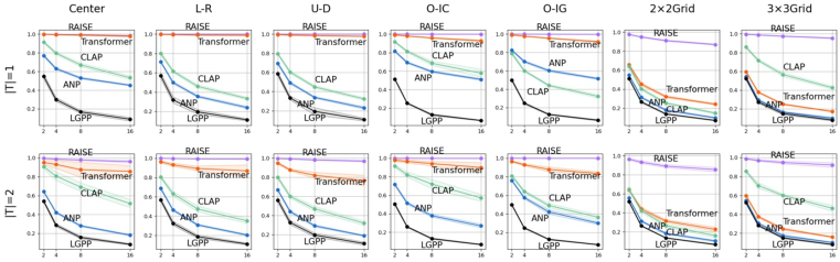
Figure 7: Selection accuracy at arbitrary positions on I-RAVEN. Each plot contains the selection accuracy of RAISE (purple), Transformer (orange), CLAP (green), ANP (blue), and LGPP (black) at arbitrary positions. The x-axis indicates the number of candidates, and the y-axis is the selection accuracy.

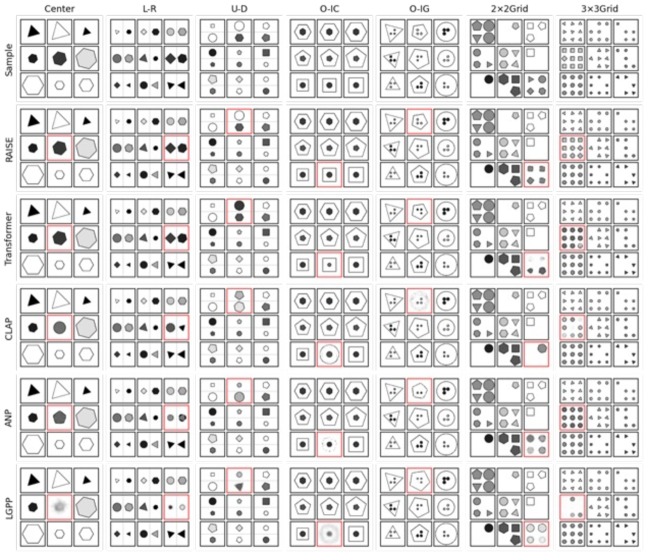
(a) The results of answer generation when $|T|=1$

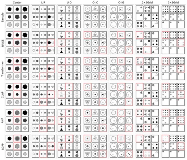
(b) The results of answer generation when $|T|=2$

Figure 8: Answer generation at arbitrary positions. The predictions are given in red boxes to illustrate the ability of (a) arbitrary-position and (b) multiple-position answer generation.

In this subsection, we give additional experimental results of answer generation at arbitrary positions. Figure 8 provides the detailed results of arbitrary-position answer generation for all seven configurations of RAVEN, for example, the prediction results when $|T|=1$ (Figure 8a) and $|T|=2$ (Figure 8b). In the visualization results, RAISE can generate high-quality predictions when $|T|=1$ and $|T|=2$. The performance of Transformer varies significantly among different configurations. Transformer predicts accurate answers on Center, while the predictions on 3$\times$3Grid deviate a lot from the ground truth images. In most cases, ANP, LGPP, and CLAP tend to generate incorrect images. Figure 7 provides the selection accuracy on I-RAVEN with different numbers of targets ($|T|=1,2$) and different sizes of candidate sets ($N_{c}=1,3,7,15$) as additional results. And we can conduct further analysis through the selection accuracy with test errors in Tables 7 and 8, where RAISE clearly outperforms other baseline models on all image configurations of RAVEN and I-RAVEN.

D.3 Latent Concepts

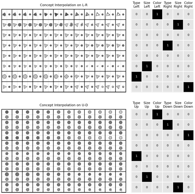
Figure 9: Concept learning on RAVEN. The table shows the interpolation results of latent concepts and the binary matrices learned in the ELBO to indicate the correspondence between concepts and attributes on L-R and U-D.

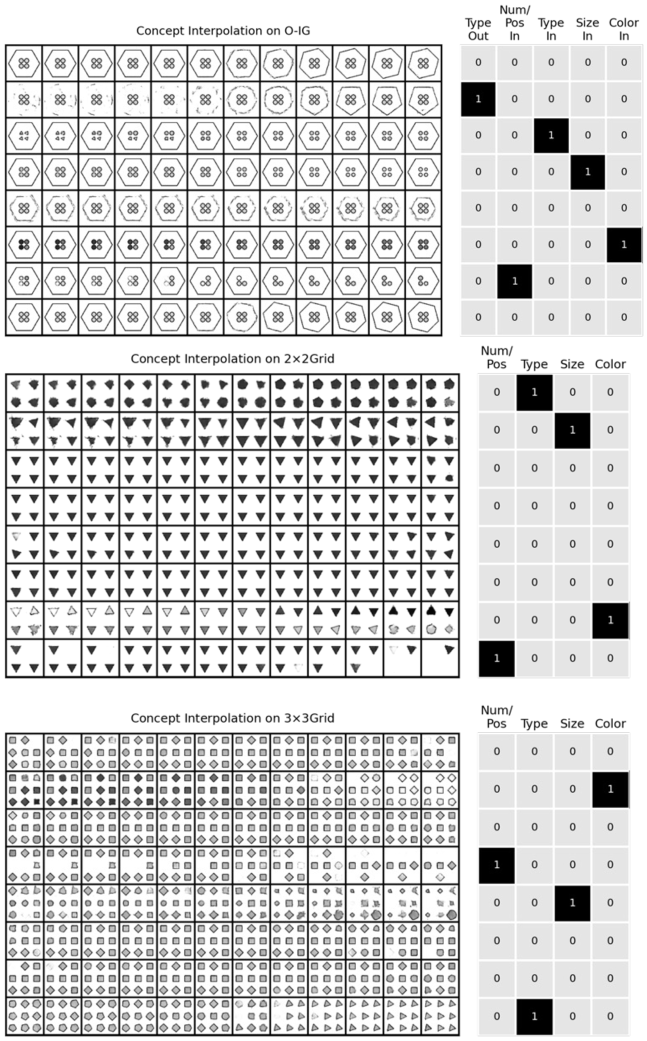
Figure 10: Concept learning on RAVEN. The table shows the interpolation results of latent concepts and the binary matrices learned in the ELBO to indicate the correspondence between concepts and attributes on O-IG, 2$\times$2Grid, and 3$\times$3Grid.

As mentioned in the main text, concept learning is an important component of RAISE. This section shows the interpolation results of latent concepts on all image configurations and the correspondences between latent concepts and real attributes in Figures 9 and 10. In most cases, RAISE learns independent latent concepts and the binary matrix $\bm{M}$ that can accurately reflect the concept-attribute correspondences. RAISE does not assign the latent concepts encoding object rotations to any attribute since the noise attributes are not included in rule annotations. This experiment illustrates the interpretability of the latent concepts, which benefits the prediction of correct answers and the following experiment of odd-one-out.

D.4 Odd-one-out in RPM

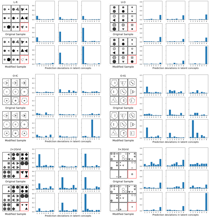
Figure 11: Odd-one-out based on RPMs. The plots display how to construct odd-one-out tests from different configurations of RPMs and how to find the odd image from the prediction deviations in concepts.

In this experiment, we give the additional results of odd-one-out on different configurations where RAISE picks out odd images interpretably via prediction deviations of concepts. Figure 11 visualizes the experimental results of the odd-one-out problems. We observe that RAISE will display larger deviations at odd concepts, which is important evidence when solving odd-one-out problems. It should be pointed out that forming such concept-level prediction deviations requires the model to parse independent concepts correctly. RAISE can apply the atomic rules in the global knowledge set to tasks like out-one-out and has interpretability in generative abstract reasoning.

D.5 Strategy of Answer Selection

Table 6: The accuracy (%) of RAISE using different answer selection strategies.

Models	Average	Center	L-R	U-D	O-IC	O-IG	2$\times$2Grid	3$\times$3Grid
RAISE-latent	90.0/92.1	99.2/99.8	98.5/99.6	99.3/99.9	97.6/99.6	89.3/96.0	68.2/71.3	77.7/78.7
RAISE-pixel	72.9/77.8	95.2/96.8	90.6/95.8	96.6/98.5	80.4/90.6	69.1/81.1	40.1/42.6	38.1/39.5

In this experiment, we evaluate RAISE with two strategies of answer selection: comparing candidates and predictions in pixel space (RAISE-pixel) and latent space (RAISE-latent). The experimental results are given in Table 6, which reports higher accuracy when candidates and predictions are compared in latent space. Due to the noise in attributes, there can be multiple solutions to a generative RPM problem. Let the answer of an RPM be the image having two triangles. By generating two triangles in various positions, the answer images may significantly differ from each other in the pixel space. However, they still point to the same concepts Number=2 and Shape=Triangle in the latent space. Therefore, RAISE selects answers by comparing candidates and predictions in the latent space rather than the pixel space.

Table 7: Answer generation at arbitrary positions on RAVEN. We provide the average accuracy (%) and test errors (%) of ten trials on RAVEN for RAISE and baselines.

	Center $(|T|=1)$				Center $(|T|=2)$
Model	$N_{c}=1$	$N_{c}=3$	$N_{c}=7$	$N_{c}=15$	$N_{c}=1$	$N_{c}=3$	$N_{c}=7$	$N_{c}=15$
LGPP	55.8 $\pm$ 2.5	30.8 $\pm$ 1.9	17.1 $\pm$ 2.0	9.1 $\pm$ 1.2	53.8 $\pm$ 1.4	28.9 $\pm$ 1.6	15.4 $\pm$ 1.2	8.3 $\pm$ 0.6
ANP	61.4 $\pm$ 0.7	38.0 $\pm$ 0.7	23.5 $\pm$ 0.9	14.5 $\pm$ 0.7	58.3 $\pm$ 0.5	34.7 $\pm$ 1.3	20.5 $\pm$ 1.0	12.2 $\pm$ 0.7
CLAP	91.5 $\pm$ 0.7	80.1 $\pm$ 1.6	67.2 $\pm$ 1.8	53.8 $\pm$ 1.7	90.8 $\pm$ 2.1	80.3 $\pm$ 3.4	67.7 $\pm$ 6.0	55.3 $\pm$ 6.2
Transformer	99.6 $\pm$ 0.2	99.1 $\pm$ 0.2	98.5 $\pm$ 0.3	97.3 $\pm$ 0.5	97.2 $\pm$ 2.3	91.1 $\pm$ 5.7	88.0 $\pm$ 4.0	90.2 $\pm$ 5.5
RAISE	99.9 $\pm$ 0.1	99.6 $\pm$ 0.2	99.1 $\pm$ 0.2	98.1 $\pm$ 0.3	99.5 $\pm$ 0.2	98.7 $\pm$ 0.3	97.5 $\pm$ 0.7	96.5 $\pm$ 0.5
	L-R $(|T|=1)$				L-R $(|T|=2)$
Model	$N_{c}=1$	$N_{c}=3$	$N_{c}=7$	$N_{c}=15$	$N_{c}=1$	$N_{c}=3$	$N_{c}=7$	$N_{c}=15$
LGPP	56.8 $\pm$ 2.3	32.7 $\pm$ 3.2	18.7 $\pm$ 2.0	9.6 $\pm$ 1.3	57.4 $\pm$ 2.1	31.9 $\pm$ 1.9	18.4 $\pm$ 2.0	9.4 $\pm$ 1.1
ANP	59.0 $\pm$ 0.6	34.6 $\pm$ 1.4	20.6 $\pm$ 0.9	11.7 $\pm$ 0.5	60.5 $\pm$ 1.2	36.3 $\pm$ 1.1	21.7 $\pm$ 0.9	12.6 $\pm$ 0.7
CLAP	79.5 $\pm$ 0.9	60.7 $\pm$ 1.2	45.6 $\pm$ 1.3	32.4 $\pm$ 0.9	80.3 $\pm$ 1.3	62.6 $\pm$ 2.6	46.4 $\pm$ 3.8	33.9 $\pm$ 2.6
Transformer	99.4 $\pm$ 0.2	98.8 $\pm$ 0.3	98.1 $\pm$ 0.4	97.1 $\pm$ 0.3	95.8 $\pm$ 1.6	90.5 $\pm$ 2.3	87.2 $\pm$ 2.8	81.4 $\pm$ 4.9
RAISE	99.9 $\pm$ 0.0	99.9 $\pm$ 0.0	99.9 $\pm$ 0.0	99.9 $\pm$ 0.1	99.9 $\pm$ 0.1	99.7 $\pm$ 0.2	99.3 $\pm$ 0.4	98.8 $\pm$ 0.7
	U-D $(|T|=1)$				U-D $(|T|=2)$
Model	$N_{c}=1$	$N_{c}=3$	$N_{c}=7$	$N_{c}=15$	$N_{c}=1$	$N_{c}=3$	$N_{c}=7$	$N_{c}=15$
LGPP	57.5 $\pm$ 2.3	32.8 $\pm$ 2.0	19.7 $\pm$ 4.1	10.3 $\pm$ 1.3	57.6 $\pm$ 1.5	32.5 $\pm$ 1.5	18.0 $\pm$ 1.2	10.2 $\pm$ 1.1
ANP	58.3 $\pm$ 1.1	34.3 $\pm$ 0.6	19.4 $\pm$ 0.8	10.7 $\pm$ 0.9	59.6 $\pm$ 0.6	35.6 $\pm$ 1.4	20.8 $\pm$ 0.5	11.9 $\pm$ 0.8
CLAP	78.8 $\pm$ 0.7	59.1 $\pm$ 1.2	43.1 $\pm$ 1.3	30.2 $\pm$ 1.1	78.4 $\pm$ 1.6	59.9 $\pm$ 2.8	42.9 $\pm$ 2.8	31.5 $\pm$ 2.8
Transformer	98.9 $\pm$ 0.2	97.9 $\pm$ 0.3	96.5 $\pm$ 0.4	94.8 $\pm$ 0.3	92.3 $\pm$ 1.7	85.2 $\pm$ 1.7	75.6 $\pm$ 3.1	70.6 $\pm$ 1.9
RAISE	99.9 $\pm$ 0.0	99.9 $\pm$ 0.0	99.9 $\pm$ 0.0	99.9 $\pm$ 0.0	99.6 $\pm$ 0.2	99.1 $\pm$ 0.3	98.2 $\pm$ 0.5	97.1 $\pm$ 1.1
	O-IC $(|T|=1)$				O-IC $(|T|=2)$
Model	$N_{c}=1$	$N_{c}=3$	$N_{c}=7$	$N_{c}=15$	$N_{c}=1$	$N_{c}=3$	$N_{c}=7$	$N_{c}=15$
LGPP	50.5 $\pm$ 1.3	25.8 $\pm$ 0.5	13.2 $\pm$ 0.7	6.6 $\pm$ 0.5	49.8 $\pm$ 1.3	25.7 $\pm$ 1.1	12.8 $\pm$ 0.5	6.7 $\pm$ 0.4
ANP	62.0 $\pm$ 1.2	39.8 $\pm$ 0.7	26.5 $\pm$ 0.6	17.1 $\pm$ 0.6	61.6 $\pm$ 1.1	38.6 $\pm$ 1.3	24.3 $\pm$ 1.2	15.2 $\pm$ 0.9
CLAP	91.3 $\pm$ 1.1	81.1 $\pm$ 1.8	68.1 $\pm$ 2.2	54.1 $\pm$ 2.2	90.9 $\pm$ 2.2	81.4 $\pm$ 2.4	68.8 $\pm$ 4.8	57.5 $\pm$ 6.5
Transformer	97.6 $\pm$ 0.4	95.0 $\pm$ 0.6	90.1 $\pm$ 0.5	82.3 $\pm$ 0.7	96.7 $\pm$ 1.7	92.1 $\pm$ 3.3	90.2 $\pm$ 3.8	80.2 $\pm$ 5.0
RAISE	99.9 $\pm$ 0.0	99.9 $\pm$ 0.0	99.9 $\pm$ 0.1	99.8 $\pm$ 0.1	99.9 $\pm$ 0.0	99.9 $\pm$ 0.1	99.9 $\pm$ 0.2	99.8 $\pm$ 0.1
	O-IG $(|T|=1)$				O-IG $(|T|=2)$
Model	$N_{c}=1$	$N_{c}=3$	$N_{c}=7$	$N_{c}=15$	$N_{c}=1$	$N_{c}=3$	$N_{c}=7$	$N_{c}=15$
LGPP	49.9 $\pm$ 0.6	25.0 $\pm$ 1.2	12.0 $\pm$ 0.6	6.1 $\pm$ 0.3	50.0 $\pm$ 0.9	25.1 $\pm$ 1.2	12.1 $\pm$ 0.7	6.4 $\pm$ 0.5
ANP	66.1 $\pm$ 1.1	45.1 $\pm$ 1.1	30.1 $\pm$ 2.0	20.2 $\pm$ 0.5	66.5 $\pm$ 1.0	44.0 $\pm$ 1.4	28.5 $\pm$ 0.8	18.0 $\pm$ 0.9
CLAP	77.8 $\pm$ 1.5	58.4 $\pm$ 1.8	43.2 $\pm$ 1.9	30.5 $\pm$ 1.0	80.5 $\pm$ 1.6	63.1 $\pm$ 3.4	47.6 $\pm$ 3.2	35.2 $\pm$ 2.4
Transformer	97.9 $\pm$ 0.4	95.2 $\pm$ 0.5	90.6 $\pm$ 0.9	82.8 $\pm$ 0.9	93.2 $\pm$ 1.7	88.5 $\pm$ 1.6	80.4 $\pm$ 3.7	75.5 $\pm$ 3.8
RAISE	99.9 $\pm$ 0.0	99.9 $\pm$ 0.1	99.7 $\pm$ 0.1	99.5 $\pm$ 0.3	99.9 $\pm$ 0.0	99.9 $\pm$ 0.0	99.9 $\pm$ 0.1	99.9 $\pm$ 0.1
	2$\times$2Grid $(|T|=1)$				2$\times$2Grid $(|T|=2)$
Model	$N_{c}=1$	$N_{c}=3$	$N_{c}=7$	$N_{c}=15$	$N_{c}=1$	$N_{c}=3$	$N_{c}=7$	$N_{c}=15$
LGPP	51.3 $\pm$ 1.0	26.7 $\pm$ 0.7	13.6 $\pm$ 0.8	6.9 $\pm$ 0.6	52.6 $\pm$ 1.4	27.0 $\pm$ 0.9	13.8 $\pm$ 0.7	7.2 $\pm$ 0.6
ANP	54.8 $\pm$ 0.9	30.8 $\pm$ 0.7	18.2 $\pm$ 0.5	9.5 $\pm$ 0.6	55.5 $\pm$ 1.0	31.7 $\pm$ 0.8	18.4 $\pm$ 0.8	10.5 $\pm$ 0.6
CLAP	64.5 $\pm$ 1.1	39.9 $\pm$ 1.5	24.5 $\pm$ 1.2	15.0 $\pm$ 0.9	64.9 $\pm$ 1.9	41.8 $\pm$ 1.5	25.2 $\pm$ 1.5	16.9 $\pm$ 1.4
Transformer	64.3 $\pm$ 1.2	44.0 $\pm$ 1.4	30.3 $\pm$ 1.5	21.6 $\pm$ 1.2	63.1 $\pm$ 1.0	43.3 $\pm$ 1.5	28.8 $\pm$ 1.4	20.9 $\pm$ 1.5
RAISE	97.2 $\pm$ 0.3	93.5 $\pm$ 0.7	89.8 $\pm$ 0.6	85.9 $\pm$ 1.1	96.5 $\pm$ 0.4	92.1 $\pm$ 1.9	87.5 $\pm$ 2.1	83.2 $\pm$ 1.7
	3$\times$3Grid $(|T|=1)$				3$\times$3Grid $(|T|=2)$
Model	$N_{c}=1$	$N_{c}=3$	$N_{c}=7$	$N_{c}=15$	$N_{c}=1$	$N_{c}=3$	$N_{c}=7$	$N_{c}=15$
LGPP	53.2 $\pm$ 1.3	28.3 $\pm$ 0.9	14.8 $\pm$ 0.4	8.1 $\pm$ 1.0	52.8 $\pm$ 1.2	27.9 $\pm$ 1.2	14.8 $\pm$ 0.9	7.8 $\pm$ 0.6
ANP	53.9 $\pm$ 1.0	29.7 $\pm$ 0.9	16.7 $\pm$ 0.2	9.4 $\pm$ 0.7	55.0 $\pm$ 1.2	31.3 $\pm$ 1.4	17.9 $\pm$ 0.7	10.4 $\pm$ 0.4
CLAP	86.2 $\pm$ 1.0	71.2 $\pm$ 1.3	56.4 $\pm$ 1.8	43.9 $\pm$ 1.2	86.1 $\pm$ 1.3	72.3 $\pm$ 2.8	60.9 $\pm$ 3.4	47.1 $\pm$ 4.0
Transformer	59.4 $\pm$ 0.8	37.8 $\pm$ 1.1	24.3 $\pm$ 0.8	16.2 $\pm$ 0.4	59.5 $\pm$ 0.8	36.6 $\pm$ 1.3	23.6 $\pm$ 0.8	16.4 $\pm$ 1.1
RAISE	99.5 $\pm$ 0.2	98.5 $\pm$ 0.2	97.0 $\pm$ 0.2	95.1 $\pm$ 0.6	98.4 $\pm$ 0.4	97.2 $\pm$ 1.0	95.4 $\pm$ 1.0	93.6 $\pm$ 1.2

Table 8: Answer generation at arbitrary positions on I-RAVEN. We provide the average accuracy (%) and test errors (%) of ten trials on I-RAVEN for RAISE and baselines.

	Center $(|T|=1)$				Center $(|T|=2)$
Model	$N_{c}=1$	$N_{c}=3$	$N_{c}=7$	$N_{c}=15$	$N_{c}=1$	$N_{c}=3$	$N_{c}=7$	$N_{c}=15$
LGPP	55.0 $\pm$ 2.9	30.0 $\pm$ 2.1	16.8 $\pm$ 1.6	9.0 $\pm$ 1.9	54.3 $\pm$ 1.3	28.7 $\pm$ 1.5	15.7 $\pm$ 1.4	8.4 $\pm$ 0.8
ANP	77.1 $\pm$ 1.2	63.1 $\pm$ 1.0	53.0 $\pm$ 1.1	45.3 $\pm$ 0.7	64.5 $\pm$ 0.8	42.3 $\pm$ 1.0	28.0 $\pm$ 0.8	18.1 $\pm$ 0.8
CLAP	91.6 $\pm$ 1.3	79.6 $\pm$ 1.3	67.1 $\pm$ 2.0	53.4 $\pm$ 1.9	90.8 $\pm$ 2.2	80.8 $\pm$ 4.6	69.2 $\pm$ 4.4	51.7 $\pm$ 4.2
Transformer	99.8 $\pm$ 0.1	99.4 $\pm$ 0.2	98.9 $\pm$ 0.3	97.8 $\pm$ 0.5	95.2 $\pm$ 2.2	93.1 $\pm$ 4.2	87.6 $\pm$ 7.9	85.8 $\pm$ 6.1
RAISE	99.9 $\pm$ 0.1	99.7 $\pm$ 0.1	99.3 $\pm$ 0.2	98.3 $\pm$ 0.3	99.5 $\pm$ 0.2	98.8 $\pm$ 0.4	97.8 $\pm$ 0.4	96.1 $\pm$ 1.3
	L-R $(|T|=1)$				L-R $(|T|=2)$
Model	$N_{c}=1$	$N_{c}=3$	$N_{c}=7$	$N_{c}=15$	$N_{c}=1$	$N_{c}=3$	$N_{c}=7$	$N_{c}=15$
LGPP	57.1 $\pm$ 2.9	31.9 $\pm$ 3.3	19.4 $\pm$ 2.3	11.2 $\pm$ 1.1	56.7 $\pm$ 1.9	32.5 $\pm$ 2.2	18.7 $\pm$ 1.7	11.0 $\pm$ 1.0
ANP	71.4 $\pm$ 1.0	49.8 $\pm$ 1.3	35.4 $\pm$ 1.0	24.0 $\pm$ 1.3	68.7 $\pm$ 1.3	46.3 $\pm$ 1.0	30.8 $\pm$ 0.8	20.4 $\pm$ 0.9
CLAP	80.0 $\pm$ 1.6	61.5 $\pm$ 1.3	45.9 $\pm$ 1.7	33.3 $\pm$ 1.3	80.5 $\pm$ 1.6	63.2 $\pm$ 2.6	47.4 $\pm$ 2.8	35.1 $\pm$ 2.5
Transformer	99.7 $\pm$ 0.1	99.4 $\pm$ 0.1	99.0 $\pm$ 0.2	98.8 $\pm$ 0.3	96.4 $\pm$ 1.3	93.1 $\pm$ 1.6	89.3 $\pm$ 2.5	86.9 $\pm$ 6.1
RAISE	99.9 $\pm$ 0.0	99.9 $\pm$ 0.0	99.9 $\pm$ 0.0	99.9 $\pm$ 0.0	99.9 $\pm$ 0.1	99.7 $\pm$ 0.1	99.4 $\pm$ 0.3	99.3 $\pm$ 0.5
	U-D $(|T|=1)$				U-D $(|T|=2)$
Model	$N_{c}=1$	$N_{c}=3$	$N_{c}=7$	$N_{c}=15$	$N_{c}=1$	$N_{c}=3$	$N_{c}=7$	$N_{c}=15$
LGPP	58.5 $\pm$ 2.5	33.3 $\pm$ 2.0	19.2 $\pm$ 3.8	10.8 $\pm$ 1.5	56.1 $\pm$ 2.6	32.6 $\pm$ 2.2	19.6 $\pm$ 2.0	10.7 $\pm$ 1.5
ANP	69.5 $\pm$ 1.4	49.1 $\pm$ 1.2	33.8 $\pm$ 0.9	23.0 $\pm$ 1.3	66.7 $\pm$ 1.1	44.1 $\pm$ 1.3	29.2 $\pm$ 1.1	18.9 $\pm$ 0.6
CLAP	79.5 $\pm$ 0.9	60.4 $\pm$ 1.5	44.8 $\pm$ 1.4	32.3 $\pm$ 1.4	79.8 $\pm$ 2.0	59.9 $\pm$ 2.0	47.0 $\pm$ 2.4	32.0 $\pm$ 2.4
Transformer	99.5 $\pm$ 0.1	99.0 $\pm$ 0.3	98.5 $\pm$ 0.4	97.7 $\pm$ 0.3	94.8 $\pm$ 1.2	87.6 $\pm$ 1.0	82.0 $\pm$ 3.1	76.5 $\pm$ 5.5
RAISE	99.9 $\pm$ 0.0	99.9 $\pm$ 0.0	99.9 $\pm$ 0.0	99.9 $\pm$ 0.0	99.6 $\pm$ 0.2	99.1 $\pm$ 0.3	98.1 $\pm$ 0.5	96.9 $\pm$ 0.8
	O-IC $(|T|=1)$				O-IC $(|T|=2)$
Model	$N_{c}=1$	$N_{c}=3$	$N_{c}=7$	$N_{c}=15$	$N_{c}=1$	$N_{c}=3$	$N_{c}=7$	$N_{c}=15$
LGPP	51.4 $\pm$ 1.0	25.4 $\pm$ 0.7	12.9 $\pm$ 0.9	6.7 $\pm$ 0.5	50.5 $\pm$ 1.3	25.8 $\pm$ 0.7	13.1 $\pm$ 0.7	6.6 $\pm$ 0.5
ANP	81.5 $\pm$ 0.7	69.4 $\pm$ 1.0	59.5 $\pm$ 0.9	51.1 $\pm$ 1.1	71.6 $\pm$ 1.2	51.5 $\pm$ 1.3	37.9 $\pm$ 1.6	26.9 $\pm$ 2.0
CLAP	91.7 $\pm$ 0.9	81.4 $\pm$ 1.3	68.6 $\pm$ 2.3	57.8 $\pm$ 4.3	91.5 $\pm$ 1.6	82.3 $\pm$ 2.7	72.1 $\pm$ 4.9	57.1 $\pm$ 3.7
Transformer	99.1 $\pm$ 0.2	98.0 $\pm$ 0.3	95.9 $\pm$ 0.4	92.9 $\pm$ 0.9	97.9 $\pm$ 1.5	96.6 $\pm$ 1.6	94.2 $\pm$ 2.5	90.0 $\pm$ 5.2
RAISE	99.9 $\pm$ 0.0	99.9 $\pm$ 0.0	99.9 $\pm$ 0.1	99.9 $\pm$ 0.1	99.9 $\pm$ 0.0	99.9 $\pm$ 0.0	99.9 $\pm$ 0.1	99.8 $\pm$ 0.1
	O-IG $(|T|=1)$				O-IG $(|T|=2)$
Model	$N_{c}=1$	$N_{c}=3$	$N_{c}=7$	$N_{c}=15$	$N_{c}=1$	$N_{c}=3$	$N_{c}=7$	$N_{c}=15$
LGPP	50.0 $\pm$ 1.3	24.8 $\pm$ 1.0	12.6 $\pm$ 0.6	6.2 $\pm$ 0.7	49.7 $\pm$ 0.7	24.9 $\pm$ 0.8	12.4 $\pm$ 0.6	6.7 $\pm$ 0.4
ANP	82.6 $\pm$ 0.7	70.2 $\pm$ 1.1	60.3 $\pm$ 1.2	51.5 $\pm$ 0.9	75.9 $\pm$ 0.8	57.5 $\pm$ 1.2	42.1 $\pm$ 2.4	29.9 $\pm$ 1.5
CLAP	79.0 $\pm$ 1.8	60.2 $\pm$ 1.1	44.2 $\pm$ 1.1	32.2 $\pm$ 1.9	81.0 $\pm$ 1.7	64.2 $\pm$ 1.3	49.0 $\pm$ 2.1	36.4 $\pm$ 2.6
Transformer	99.0 $\pm$ 0.3	97.8 $\pm$ 0.3	95.6 $\pm$ 0.4	91.8 $\pm$ 0.7	96.6 $\pm$ 0.9	93.0 $\pm$ 1.1	87.9 $\pm$ 2.5	83.5 $\pm$ 1.8
RAISE	99.9 $\pm$ 0.0	99.9 $\pm$ 0.0	99.9 $\pm$ 0.1	99.8 $\pm$ 0.1	99.9 $\pm$ 0.0	99.9 $\pm$ 0.1	99.9 $\pm$ 0.1	99.9 $\pm$ 0.1
	2$\times$2Grid $(|T|=1)$				2$\times$2Grid $(|T|=2)$
Model	$N_{c}=1$	$N_{c}=3$	$N_{c}=7$	$N_{c}=15$	$N_{c}=1$	$N_{c}=3$	$N_{c}=7$	$N_{c}=15$
LGPP	51.3 $\pm$ 0.8	26.6 $\pm$ 1.0	13.9 $\pm$ 0.5	7.1 $\pm$ 0.5	51.9 $\pm$ 1.0	26.4 $\pm$ 0.6	13.7 $\pm$ 0.4	6.8 $\pm$ 0.5
ANP	54.9 $\pm$ 1.0	31.4 $\pm$ 1.0	18.0 $\pm$ 1.0	9.9 $\pm$ 0.7	55.6 $\pm$ 0.7	31.4 $\pm$ 0.9	18.4 $\pm$ 1.0	10.5 $\pm$ 1.0
CLAP	63.9 $\pm$ 1.4	40.2 $\pm$ 1.5	25.4 $\pm$ 1.2	14.8 $\pm$ 1.0	64.8 $\pm$ 1.7	42.5 $\pm$ 2.0	26.6 $\pm$ 1.8	16.1 $\pm$ 2.1
Transformer	65.7 $\pm$ 1.4	45.3 $\pm$ 1.4	32.1 $\pm$ 1.1	24.2 $\pm$ 0.8	64.2 $\pm$ 0.3	44.1 $\pm$ 1.9	31.5 $\pm$ 1.4	22.7 $\pm$ 2.2
RAISE	97.5 $\pm$ 0.4	95.0 $\pm$ 0.6	91.1 $\pm$ 0.7	87.0 $\pm$ 0.7	96.4 $\pm$ 0.9	93.2 $\pm$ 1.4	89.0 $\pm$ 1.6	85.5 $\pm$ 2.3
	3$\times$3Grid $(|T|=1)$				3$\times$3Grid $(|T|=2)$
Model	$N_{c}=1$	$N_{c}=3$	$N_{c}=7$	$N_{c}=15$	$N_{c}=1$	$N_{c}=3$	$N_{c}=7$	$N_{c}=15$
LGPP	52.4 $\pm$ 1.3	27.2 $\pm$ 1.3	14.9 $\pm$ 1.4	8.0 $\pm$ 0.9	52.4 $\pm$ 1.0	28.2 $\pm$ 0.9	15.0 $\pm$ 0.8	8.1 $\pm$ 0.6
ANP	54.2 $\pm$ 1.2	29.5 $\pm$ 1.0	16.6 $\pm$ 0.8	10.1 $\pm$ 0.9	54.5 $\pm$ 1.1	30.6 $\pm$ 0.7	17.4 $\pm$ 1.1	10.2 $\pm$ 0.5
CLAP	85.9 $\pm$ 1.2	71.7 $\pm$ 1.3	56.6 $\pm$ 2.0	42.6 $\pm$ 1.5	85.6 $\pm$ 1.1	70.4 $\pm$ 3.0	60.0 $\pm$ 1.2	46.4 $\pm$ 3.0
Transformer	59.7 $\pm$ 1.3	37.7 $\pm$ 0.8	25.0 $\pm$ 0.7	17.2 $\pm$ 0.5	59.7 $\pm$ 1.0	37.4 $\pm$ 1.0	24.5 $\pm$ 1.1	16.0 $\pm$ 0.6
RAISE	99.6 $\pm$ 0.1	98.8 $\pm$ 0.2	97.5 $\pm$ 0.3	95.5 $\pm$ 0.6	98.8 $\pm$ 0.5	97.0 $\pm$ 0.9	94.8 $\pm$ 1.5	92.2 $\pm$ 2.5

appendix iclr2024_conference

References

- Barrett et al. (2018) David Barrett, Felix Hill, Adam Santoro, Ari Morcos, and Timothy Lillicrap. Measuring abstract reasoning in neural networks. In International conference on machine learning, pp. 511–520. PMLR, 2018.
- Benny et al. (2021) Yaniv Benny, Niv Pekar, and Lior Wolf. Scale-localized abstract reasoning. In Proceedings of the IEEE/CVF Conference on Computer Vision and Pattern Recognition, pp. 12557–12565, 2021.
- Byrne & Johnson-Laird (1989) Ruth MJ Byrne and Philip N Johnson-Laird. Spatial reasoning. Journal of memory and language, 28(5):564–575, 1989.
- Cattell (1963) Raymond B Cattell. Theory of fluid and crystallized intelligence: A critical experiment. Journal of educational psychology, 54(1):1, 1963.
- Chen et al. (2021) Chang Chen, Fei Deng, and Sungjin Ahn. Roots: Object-centric representation and rendering of 3d scenes. The Journal of Machine Learning Research, 22(1):11770–11805, 2021.
- Chollet (2019) François Chollet. On the measure of intelligence. arXiv preprint arXiv:1911.01547, 2019.
- Crouse (2016) David F Crouse. On implementing 2d rectangular assignment algorithms. IEEE Transactions on Aerospace and Electronic Systems, 52(4):1679–1696, 2016.
- Dehaene (2011) Stanislas Dehaene. The number sense: How the mind creates mathematics. OUP USA, 2011.
- Edwards & Storkey (2017) Harrison Edwards and Amos Storkey. Towards a neural statistician. In International Conference on Learning Representations, 2017.
- Eslami et al. (2018) SM Ali Eslami, Danilo Jimenez Rezende, Frederic Besse, Fabio Viola, Ari S Morcos, Marta Garnelo, Avraham Ruderman, Andrei A Rusu, Ivo Danihelka, Karol Gregor, et al. Neural scene representation and rendering. Science, 360(6394):1204–1210, 2018.
- Foong et al. (2020) Andrew Foong, Wessel Bruinsma, Jonathan Gordon, Yann Dubois, James Requeima, and Richard Turner. Meta-learning stationary stochastic process prediction with convolutional neural processes. Advances in Neural Information Processing Systems, 33:8284–8295, 2020.
- Gao & Li (2023) Chengmin Gao and Bin Li. Time-conditioned generative modeling of object-centric representations for video decomposition and prediction. In Proceedings of the Conference on Uncertainty in Artificial Intelligence, pp. 613–623, 2023.
- Garnelo et al. (2018) Marta Garnelo, Jonathan Schwarz, Dan Rosenbaum, Fabio Viola, Danilo J Rezende, SM Eslami, and Yee Whye Teh. Neural processes. In ICML 2018 Workshop on Theoretical Foundations and Applications of Deep Generative Models, 2018.
- Giannone & Winther (2021) Giorgio Giannone and Ole Winther. Hierarchical few-shot generative models. In Fifth Workshop on Meta-Learning at the Conference on Neural Information Processing Systems, 2021.
- Gordon & Irwin (1996) Robert D Gordon and David E Irwin. What’s in an object file? evidence from priming studies. Perception & Psychophysics, 58(8):1260–1277, 1996.
- Gray & Thompson (2004) Jeremy R Gray and Paul M Thompson. Neurobiology of intelligence: science and ethics. Nature Reviews Neuroscience, 5(6):471–482, 2004.
- Hahne et al. (2019) Lukas Hahne, Timo Lüddecke, Florentin Wörgötter, and David Kappel. Attention on abstract visual reasoning. arXiv preprint arXiv:1911.05990, 2019.
- Hewitt et al. (2018) Luke B Hewitt, Maxwell I Nye, Andreea Gane, Tommi S Jaakkola, and Joshua B Tenenbaum. The variational homoencoder: Learning to learn high capacity generative models from few examples. In Conference on Uncertainty in Artificial Intelligence. Association For Uncertainty in Artificial Intelligence (AUAI), 2018.
- Hu et al. (2021) Sheng Hu, Yuqing Ma, Xianglong Liu, Yanlu Wei, and Shihao Bai. Stratified rule-aware network for abstract visual reasoning. In Proceedings of the AAAI Conference on Artificial Intelligence, volume 35, pp. 1567–1574, 2021.
- Hua & Kunda (2020) Tianyu Hua and Maithilee Kunda. Modeling gestalt visual reasoning on raven’s progressive matrices using generative image inpainting techniques. In CogSci, volume 2, pp. 7, 2020.
- Jahrens & Martinetz (2020) Marius Jahrens and Thomas Martinetz. Solving raven’s progressive matrices with multi-layer relation networks. In 2020 International Joint Conference on Neural Networks (IJCNN), pp. 1–6. IEEE, 2020.
- Jiang & Ahn (2020) Jindong Jiang and Sungjin Ahn. Generative neurosymbolic machines. Advances in Neural Information Processing Systems, 33:12572–12582, 2020.
- Kabra et al. (2021) Rishabh Kabra, Daniel Zoran, Goker Erdogan, Loic Matthey, Antonia Creswell, Matt Botvinick, Alexander Lerchner, and Chris Burgess. Simone: View-invariant, temporally-abstracted object representations via unsupervised video decomposition. Advances in Neural Information Processing Systems, 34:20146–20159, 2021.
- Kahneman et al. (1992) Daniel Kahneman, Anne Treisman, and Brian J Gibbs. The reviewing of object files: Object-specific integration of information. Cognitive psychology, 24(2):175–219, 1992.
- Kim et al. (2019) Hyunjik Kim, Andriy Mnih, Jonathan Schwarz, Marta Garnelo, Ali Eslami, Dan Rosenbaum, Oriol Vinyals, and Yee Whye Teh. Attentive neural processes. In International Conference on Learning Representations, 2019.
- Kingma & Welling (2013) Diederik P Kingma and Max Welling. Auto-encoding variational bayes. arXiv preprint arXiv:1312.6114, 2013.
- Lake et al. (2011) Brenden Lake, Ruslan Salakhutdinov, Jason Gross, and Joshua Tenenbaum. One shot learning of simple visual concepts. In Proceedings of the annual meeting of the cognitive science society, volume 33, 2011.
- Locatello et al. (2020) Francesco Locatello, Dirk Weissenborn, Thomas Unterthiner, Aravindh Mahendran, Georg Heigold, Jakob Uszkoreit, Alexey Dosovitskiy, and Thomas Kipf. Object-centric learning with slot attention. Advances in Neural Information Processing Systems, 33:11525–11538, 2020.
- Małkiński & Mańdziuk (2022a) Mikołaj Małkiński and Jacek Mańdziuk. Deep learning methods for abstract visual reasoning: A survey on raven’s progressive matrices. arXiv preprint arXiv:2201.12382, 2022a.
- Małkiński & Mańdziuk (2022b) Mikołaj Małkiński and Jacek Mańdziuk. A review of emerging research directions in abstract visual reasoning. arXiv preprint arXiv:2202.10284, 2022b.
- McCloskey (1983) Michael McCloskey. Intuitive physics. Scientific american, 248(4):122–131, 1983.
- Mitchell (2021) Melanie Mitchell. Abstraction and analogy-making in artificial intelligence. Annals of the New York Academy of Sciences, 1505(1):79–101, 2021.
- Pekar et al. (2020) Niv Pekar, Yaniv Benny, and Lior Wolf. Generating correct answers for progressive matrices intelligence tests. arXiv preprint arXiv:2011.00496, 2020.
- Raven & Court (1998) John C Raven and John Hugh Court. Raven’s progressive matrices and vocabulary scales, volume 759. Oxford pyschologists Press Oxford, 1998.
- Shi et al. (2021) Fan Shi, Bin Li, and Xiangyang Xue. Raven’s progressive matrices completion with latent gaussian process priors. In Proceedings of the AAAI Conference on Artificial Intelligence, volume 35, pp. 9612–9620, 2021.
- Shi et al. (2023) Fan Shi, Bin Li, and Xiangyang Xue. Compositional law parsing with latent random functions. In International Conference on Learning Representations, 2023.
- Sohn et al. (2015) Kihyuk Sohn, Honglak Lee, and Xinchen Yan. Learning structured output representation using deep conditional generative models. Advances in neural information processing systems, 28, 2015.
- Sønderby et al. (2016) Casper Kaae Sønderby, Tapani Raiko, Lars Maaløe, Søren Kaae Sønderby, and Ole Winther. Ladder variational autoencoders. Advances in neural information processing systems, 29:3738–3746, 2016.
- Steenbrugge et al. (2018) Xander Steenbrugge, Sam Leroux, Tim Verbelen, and Bart Dhoedt. Improving generalization for abstract reasoning tasks using disentangled feature representations. arXiv preprint arXiv:1811.04784, 2018.
- Vaswani et al. (2017) Ashish Vaswani, Noam Shazeer, Niki Parmar, Jakob Uszkoreit, Llion Jones, Aidan N Gomez, Łukasz Kaiser, and Illia Polosukhin. Attention is all you need. Advances in neural information processing systems, 30, 2017.
- Wang et al. (2019) Duo Wang, Mateja Jamnik, and Pietro Lio. Abstract diagrammatic reasoning with multiplex graph networks. In International Conference on Learning Representations, 2019.
- Wang et al. (2020) Duo Wang, Mateja Jamnik, and Pietro Lio. Abstract diagrammatic reasoning with multiplex graph networks. arXiv preprint arXiv:2006.11197, 2020.
- Williams & Rasmussen (2006) Christopher K Williams and Carl Edward Rasmussen. Gaussian processes for machine learning, volume 2. MIT press Cambridge, MA, 2006.
- Wu et al. (2020) Yuhuai Wu, Honghua Dong, Roger Grosse, and Jimmy Ba. The scattering compositional learner: Discovering objects, attributes, relationships in analogical reasoning. arXiv preprint arXiv:2007.04212, 2020.
- Yuan et al. (2022) Jinyang Yuan, Bin Li, and Xiangyang Xue. Unsupervised learning of compositional scene representations from multiple unspecified viewpoints. In Proceedings of the AAAI Conference on Artificial Intelligence, volume 36, pp. 8971–8979, 2022.
- Yuan et al. (2023) Jinyang Yuan, Tonglin Chen, Bin Li, and Xiangyang Xue. Compositional scene representation learning via reconstruction: A survey. IEEE Transactions on Pattern Analysis & Machine Intelligence, 45(10):11540–11560, 2023.
- Yuan et al. (in press) Jinyang Yuan, Tonglin Chen, Zhimeng Shen, Bin Li, and Xiangyang Xue. Unsupervised object-centric learning from multiple unspecified viewpoints. IEEE Transactions on Pattern Analysis & Machine Intelligence, in press.
- Zhang et al. (2019a) Chi Zhang, Feng Gao, Baoxiong Jia, Yixin Zhu, and Song-Chun Zhu. Raven: A dataset for relational and analogical visual reasoning. In Proceedings of the IEEE/CVF Conference on Computer Vision and Pattern Recognition, pp. 5317–5327, 2019a.
- Zhang et al. (2019b) Chi Zhang, Baoxiong Jia, Feng Gao, Yixin Zhu, Hongjing Lu, and Song-Chun Zhu. Learning perceptual inference by contrasting. arXiv preprint arXiv:1912.00086, 2019b.
- Zhang et al. (2021a) Chi Zhang, Baoxiong Jia, Song-Chun Zhu, and Yixin Zhu. Abstract spatial-temporal reasoning via probabilistic abduction and execution. In Proceedings of the IEEE/CVF Conference on Computer Vision and Pattern Recognition, pp. 9736–9746, 2021a.
- Zhang et al. (2021b) Chi Zhang, Sirui Xie, Baoxiong Jia, Ying Nian Wu, Song-Chun Zhu, and Yixin Zhu. Learning algebraic representation for systematic generalization in abstract reasoning. arXiv preprint arXiv:2111.12990, 2021b.
- Zheng et al. (2019) Kecheng Zheng, Zheng-Jun Zha, and Wei Wei. Abstract reasoning with distracting features. Advances in Neural Information Processing Systems, 32, 2019.
- Zhuo & Kankanhalli (2021) Tao Zhuo and Mohan Kankanhalli. Effective abstract reasoning with dual-contrast network. In International Conference on Learning Representations, 2021.