Resetting as a swift equilibration protocol in an anharmonic potential

Abstract

We present and characterize a method to accelerate the relaxation of a Brownian object between two distinct equilibrium states. Instead of relying on a deterministic time-dependent control parameter, we use stochastic resetting to guide and accelerate the transient evolution. The protocol is investigated numerically, and its thermodynamic cost is evaluated with the tools of stochastic thermodynamics. Remarkably, we show that stochastic resetting significantly accelerates the relaxation to the final state. This stochastic protocol exhibits energetic and temporal characteristics that align with the scales observed in previously investigated deterministic protocols. Moreover, it expands the spectrum of stationary states that can be manipulated, incorporating new potential profiles achievable through experimentally viable protocols.

Swift driving protocols in non-equilibrium statistical mechanics aim to manage a system’s transition between thermal equilibrium states efficiently, seeking quicker routes to equilibrium than natural relaxation [1, 2, 3, 4]. For instance, various techniques were used to showcase a reduction in the relaxation time ($\tau_{r}$) of a Brownian particle coupled to a thermal bath after a sudden change in a control parameter, e.g., potential stiffness or temperature. Such swift state-to-state transformation (SST) protocols usually rely on the full knowledge of the time-dependant probability density and its relation to external control parameters. This allows reverse engineering a well-chosen temporal change of the control parameter ending at the new equilibrium state [4].

In simple cases like harmonic confinement, explicit SST protocols were derived and experimentally implemented to control the relaxation of Brownian particles [5, 6, 7]. SST for arbitrary potentials [3] or between non-equilibrium states [8, 9] are more complex and challenging to implement experimentally.

The energetic expenses of these control protocols are effectively analyzed through stochastic thermodynamics [10, 11], at the level of individual stochastic trajectories. General rules of time-energy trades-offs in such protocols are thus calculated, enabling their optimization [12, 13, 14, 15].

Stochastic resetting (SR) is a driving mechanism in which a process is arrested randomly only to be re-initiated repeatedly, usually from the origin. The classic example of SR is resetting the motion of a diffusing Brownian particle [16, 17], which has been realized experimentally employing optically trapped Brownian colloidal particles [18, 19, 20], and thoroughly investigated theoretically [16, 21, 22, 23, 24, 25, 26, 27]. The rising interest in SR is prompted, among other features of SR, by the emergence of a stationary state, making SR akin to confinement yet bearing unique characteristics. Since each resetting event in SR breaks detailed balance, the resulting steady state is, of course, out of thermal equilibrium, with non-vanishing probability currents and constant dissipation of heat to the surrounding fluid [28, 29, 26, 20].

Here, we propose an innovative method to accelerate the relaxation between two states based on SR rather than on a controlled variation of the underlying potential. In our method, the potential is switched off during the transition, and the system undergoes stochastic resetting until its position distribution reaches that of the target state. Subsequently, the target potential is turned on, and the stochastic resetting is terminated.

Specifically, we demonstrate numerically that stochastic resetting accelerates the transition of a Brownian particle between two equilibrium states with a v-shaped potential. Moreover, it naturally connects two non-equilibrium steady-states where standard SSTs are difficult to derive. This method shares similarities with a previous proposal [30] where an energy-dependant SR rate, contingent upon knowledge of particle positions in time, expedites transitions between two Gaussian equilibrium states. In sharp contrast, the method developed here does not require such knowledge. Finally, we characterize the entropic cost of accelerated relaxation protocols via stochastic thermodynamics and discuss an extension to finite-time resetting, offering experimentally feasible acceleration.

Tailoring identical position distribution for equilibrium and driven systems - We start by considering a Brownian particle diffusing in a linear v-shaped potential $V(x)=b|x|$, obeying the Langevin equation,

$$\dot{x}(t)=\frac{-b}{\gamma}\textrm{sgn}(x(t))+\sqrt{2D}\xi(t),$$ (1)

where $\gamma$ is the viscous drag coefficient, $\textrm{sgn}(x(t))$ is the sign function, $D=k_{B}T/\gamma$ is the diffusion coefficient with $k_{B}$ is Boltzmann’s constant and $T$ the temperature. $\xi(t)$ is a Gaussian random variable with $\langle\xi(t)\rangle=0$ and $\langle\xi(t)\xi(s)\rangle=\delta(t-s)$. The position probability density function (PDF) of the particle, according to Boltzmann statistics, is given by,

$$P_{\rm eq}=\frac{b}{2k_{B}T}e^{-\frac{b}{k_{B}T}|x|}.$$ (2)

An exemplary Langevin simulation of such a particle is depicted in Fig. 1 (a), together with its stationary position distribution. Throughout the paper, we consider a micron-sized colloidal particle at room temperature $T=300$ K with $\gamma=8\times 10^{-9}~{}\rm{kg}~{}\rm{s}^{-1}$. The PDFs (here and below) are measured on a single trajectory of $10^{7}$ time-steps of duration $dt=10^{-6}$ s.

Figure 1: (a) Time-series of position $x(t)$ obeying the Langevin process Eq. (1) at thermal equilibrium in a v-shaped potential with slope $b=0.18$ pN; the Maxwell-Boltzmann equilibrium distribution is plotted on the right. (b) Time-series of positions $x(t)$ Brownian particle undergoing stochastic resetting with $\lambda=b^{2}/\gamma k_{B}T=1$ kHz (red line). Resetting events are shown with vertical arrows, and the Laplace PDF is plotted on the right.

In the absence of an underlying potential, SR of a Brownian particle to the origin $x=0$ with resetting times drawn from a Poisson distribution, $P(t_{\rm rst})=\lambda e^{-\lambda t_{\rm rst}}$, results in the following stationary position PDF,

$$P_{s}(x)=\frac{\alpha}{2}e^{-\alpha|x|}$$ (3)

where $\alpha=\sqrt{\lambda/D}$. A typical trajectory of such a process alongside its PDF is shown in Fig. 1 (b).

Central to our proposed acceleration protocol of an SST is the fact that this probability distribution (Eq. 3) can be tuned to be identical to the equilibrium distribution of Eq. 2 by taking $b=\alpha k_{B}T$. Namely, by fixing the resetting rate to be $\lambda_{b}=b^{2}/\gamma k_{B}T$.

Figure 2: (a) Probability distribution of an equilibrium process (blue circles) and a resetting process (red triangles), along with the analytical result $P_{\rm eq}(x)=P_{s}(x)$ (black dashed line) for a single trajectory. (b) probability density current through space for the equilibrium state (blue circles) and for SR (red triangles) together with the analytical result for SR (black dashed line).

In Fig. 2(a), we show quantitatively that by installing the appropriate resetting rate $\lambda_{b}$ we obtain the expected identical Laplace PDFs for the two cases: equilibrium with a v-shape potential (Eq. 2) and Poissonian stochastic resetting (Eq. 3). Importantly, having identical PDFs does not imply similar dynamics. Under SR, a particle experiences significant jumps at each resetting event, leading to a non-zero stationary current $j_{p}(x)=\frac{1}{\gamma}\frac{dV(x)}{dx}P_{s}(x)-D\frac{dP_{s}(x)}{dx}=\frac{D\alpha^{2}}{2}\rm{sgn}(x)e^{-\alpha|x|}$, as illustrated in Fig. 2(b). This stands in stark contrast to the behavior of a particle at equilibrium. The distinct dynamics under SR enable accelerating a transition between stationary states.

Accelerating state-to-state transition - The simplest unassisted transition between two equilibrium states involves an abrupt change of the potential slope from $b(t_{i})$ to $b(t_{f})$ followed by spontaneous relaxation. Similarly, a freely diffusing particle in steady state under resetting can be subjected to a sudden change of the resetting rate from $\lambda_{b}(t_{i})=b(t_{i})^{2}/\gamma k_{B}T$ to $\lambda_{b}(t_{f})=b(t_{f})^{2}/\gamma k_{B}T$ followed by a relaxation to the new steady state.

In Fig. 3(a, b) simulation results of both protocols are compared by depicting the evolution of the PDF, for a potential quench (a), and for a SR-assisted transition (b). The position distribution is obtained from an ensemble average of $10^{5}$ independent trajectories of 2800 time-steps with $dt=10\mu\rm{s}$. While the initial and final states of both protocols have the same PDF, the rate of its evolution is different.

Figure 3: (a) Step-like change of the potential slope $b(t)$ in the absence of resetting ($\lambda=0$) and corresponding contour plot of the time-dependent probability density. (b) Step-like change in stochastic resetting rate $\lambda(t)$ in the absence of potential ($b=0$) and corresponding time-dependent probability density. (c) five distinct PDF (from blue to red) during the transient evolution of the same ensemble under SR-assisted SST, together with $f(x,t)$ (black lines) using the values $x_{0}(t)$ extracted from a fitting procedure. (d) time-dependent boundary $x_{0}(t)$ up to the limit defined by numerical precision.

The PDF $\rho(x,t)$ takes a non-trivial shape during the transient. A time-dependent second-order discontinuity $x_{0}(t)$ separates two distinct regions [31]. In an inner core region, $\rho(x<x_{0},t)$ already reached the final steady state $P_{f}(x)=\alpha(t_{f})e^{-\alpha(t_{f})|x|}/2$, while in the outer region, $\rho(x>x_{0},t)$ still follows $P_{i}(x)=\alpha(t_{i})e^{-\alpha(t_{i})|x|}/2$.

This dynamical phase transition is visible on Fig. 3 (c) where the numerically measured $\rho(x,t)$ agree with the expression

$$f(x,t)=w(x,t)P_{i}(x)+\bar{w}(x,t)e^{-[\alpha(t_{f})-\alpha(t_{i})]x_{0}(t)}P_{f}(x),$$ (4)

with $w$ a window-function obeying $w(t)=1$ for $|x|<x_{0}(t)$ and $0$ for $|x|>x_{0}(t)$, while $\bar{w}=1-w$. The time-dependent value of the boundary $x_{0}(t)$ (see Fig. 3 (d)) between the two sections of the PDF is obtained by fitting the rate function during the transient (as detailed in Supplementary Material [32]) where $x_{0}(t)$ is the only fitting parameter. The algebraic growth of the dynamical phase transition $x_{0}(t)$ prevents the definition of an unambiguous relaxation time [32, 31]; this motivates us to define relaxation as the time needed for $\rho(x,t)$ to be indistinguishable of $P_{s}(x)$ within a finite precision. We therefore quantify the acceleration induced by SR (Fig. 3 (a, b)), via the Kulback-Leibler (KL) divergence between the measured $\rho(x,t)$, and the instantaneous stationary solution $P_{s}(x)=P_{\rm eq}(x)$ under control-parameter $b(t)$ or $\lambda_{b}(t)$ reads $\mathcal{D}_{\rm KL}(\rho(x,t)\parallel P_{s}(x))=\int\rho(x,t)\ln[\rho(x,t)/P_{s}(x)]dx.$ When the control parameter is abruptly modified, $P_{s}(x)$ immediately adapts, while the system responds gradually, characterized by $\rho(x,t)$. The delay in the system’s response is well captured by $\Delta\mathcal{D}_{\rm KL}=\mathcal{D}_{\rm KL}(t)-\mathcal{D}_{\rm KL,s}$ relative measure with respect to the stationary-state value $\mathcal{D}_{\rm KL,s}$ (only measuring the numerical precision of the histogram), plotted on Fig. 4 (a). To measure the relaxation time (blue and red vertical lines) numerically, we probe the time for the first KL-point to reach its final mean steady value. Remarkably, we observe a significantly faster relaxation to the new steady state for the SR-assisted SST, with $\tau_{\rm{SR}}\approx 4.5$ ms, compared to its equilibrium counterpart, $\tau_{\rm{r}}\approx 15$ ms (Fig. 4, (a)). In other words, the non-equilibrium steady state (NESS) evolution induced by stochastic resetting is more than three times faster than the relaxation from equilibrium to equilibrium under the selected parameters.

Figure 4: (a) Relative Kullback-Leibler divergence as a measure in natural bits of the distance to stationary state for the potential quench (blue line) and SR-assisted transition (red line). Relaxation times are underlined with blue and red vertical lines. (b) Measured relaxation times $\tau_{r}$ (blue circles) and $\tau_{\rm{SR}}$ (red triangles) as a function of the final state characterized by $\lambda(t_{f})$ with constant initial $\lambda(t_{i})$ (respective $b(t_{f})$ and $b(t_{i})$). The superimposed lines correspond to theoretical characteristic times as detailed in the main text.

The SR-based acceleration method remains valid across the entire spectrum of potential changes, which we demonstrate by varying the final value of $\lambda(t_{f})$ (respectively $b(t_{f})$) with fixed $\lambda(t_{i})=200$ Hz ($b(t_{i})=0.08$ pN). The measured relaxation times are shown in Fig. 4 (b) as a function of the final resetting rate $\lambda(t_{f})$. The NESS-to-NESS transition is always faster than the equivalent potential quench for both compression and expansion.

The dependence of the relaxation time on $\lambda(t_{f})$ is different for compression and expansion. When the potential is opened, the relaxation is dominated by diffusive forces and the transient time from a state to another increases monotonically as the difference between both states increases. Hence, during expansion, we expect the transient time to depend on the difference between the initial and final characteristic times, $\propto\Delta\mathcal{T}=|\mathcal{T}_{f}-\mathcal{T}_{i}|$ (see dashed fits in Fig. 4(b)) where the typical timescale arises naturally as $\mathcal{T}=\frac{k_{B}T\gamma}{b^{2}}=\lambda_{b}^{-1}$. In contrast, for compression, there is a competition between the acceleration due to the increasing applied conservative force $\propto b(t_{f})$ and the growing difference between initial and final states. These effects are combined in a phenomenological fit $\tau_{r}\propto\frac{b(t_{i})}{b(t_{f})}\Delta\mathcal{T}$. The same competition is expected in the case of SR-induced transition, where resetting events replace the conservative force, following $\tau_{\rm SR}\propto\frac{\lambda(t_{i})}{\lambda(t_{f})}\Delta\mathcal{T}$ (see solid line fits in Fig. 4(b)) Naturally, in the limit of $\lambda(t_{f})\rightarrow\lambda(t_{i})$ the transition becomes infinitely fast for any protocol (seen as a cusp in Fig. 4(b)). These results clearly demonstrate the ability of SR to accelerate the relaxation of a thermal system via SR NESS-to-NESS transformation.

Accelerating relaxation to equilibrium and thermodynamic cost - The ability of SR to induce fast transitions between two NESS can be adapted to expedite transitions between two equilibrium states as well. SR is then used only during the transient between the two equilibrium states. The proposed protocol is comprised of the following steps (Fig. 5 (a)): (i) a thermal equilibrium state in prepared in $V(x)=b(t_{i})|x|$; (ii) the potential is switched off and SR is applied with a rate $\lambda=b(t_{f})^{2}/(k_{B}T\gamma)$ corresponding to the target state, (iii) immediately after the system has relaxed with time $\tau_{\rm{SR}}<\tau_{r}$, resetting is stopped and the potential is switched on in its final state $V(x)=b(t_{f})|x|$. Following this protocol fastens the particle’s transition to the final equilibrium state compared to a potential quench protocol (Fig. 5 (b)) and relies on the a priori knowledge of $\tau_{\rm{SR}}$.

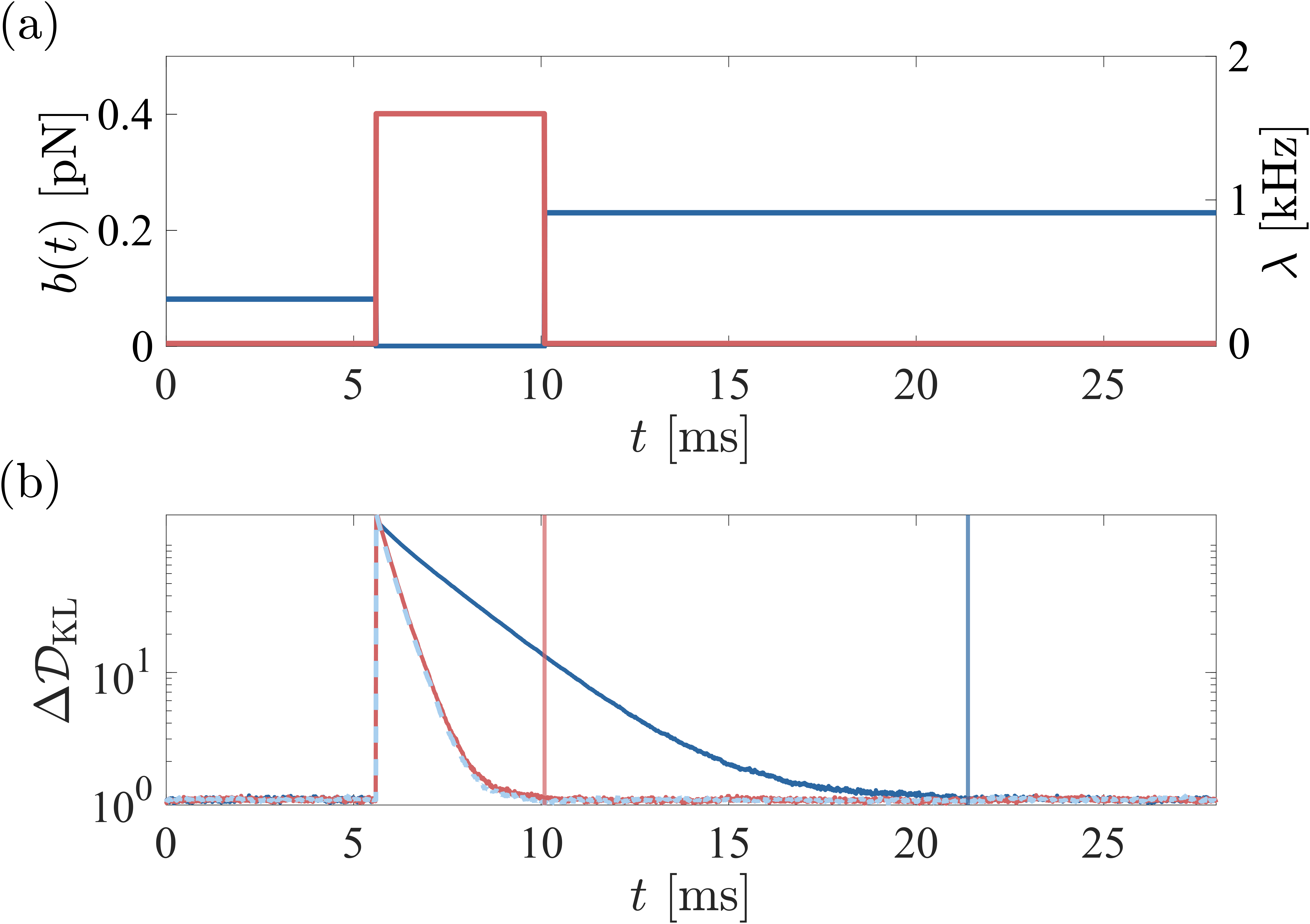
Figure 5: (a) schematic representation of the proposed protocol: initially the system is at thermal equilibrium in $V(x)=b(t_{i})|x|$, then (first black vertical line) the potential is replaced by SR with $\lambda=b(t_{f})^{2}/(k_{B}T\gamma)$ for a time $\tau_{\rm{SR}}$ and finally (second black vertical line) resetting is turned off and the system is at equilibrium in $V(x)=b(t_{f})|x|$. (b) $\Delta\mathcal{D}_{\rm KL}$ for standard potential quench (deep blue line), SR-induced NESS-to-NESS (red line) and following our protocol (light blue dashed line).

However, this approach relies on the transition from equilibrium to NESS (beginning of stage (ii)) and back (beginning of stage (iii)) to be instantaneous or with negligible time expenditure. In other words, the PDFs dynamics following this protocol should be identical for transitions between NESS and equilibrium states, which is verified in Fig. 5 (b), where the dynamics of $\mathcal{D}_{\rm KL}$ of both SR-based transitions overlap and decay faster than that of the potential quench transition between equilibrium states.

Operating through markedly different mechanisms, both protocols entail distinct thermodynamic costs [32], which we asses by comparing the total entropy produced by resetting during the transition time $\tau_{\rm SR}$, to the total entropy produced by the standard yet irreversible potential quench. We analyze here in details the various entropic contributions in both cases.

The change of steady-state distribution is accompanied by a change of ensemble-averaged system entropy [33, 11] $S_{\rm sys}=\int\rho(x,t)\ln\left(\rho(x,t)\right)dx$ (integrals span all $x$). The total contribution of the state function $\Delta S_{\rm sys}$ along the protocol only depends on initial and final PDFs and is the same whether we use a potential quench or resetting. For the potential quench, the heat dissipated in the bath yields a medium entropy $\dot{S}_{\rm m}=\dot{Q}/T$. $\dot{S}_{\rm m}$ is calculated for the potential quench protocol by identifying the heat exchanged from the Langevin equation [32] $Q=-\langle\int b(t)\rm{sgn}(x(t))\dot{x}(t)\circ dt\rangle$. Since $\dot{Q}$ vanishes in the absence of an external potential, it does not contribute to the SR-based protocol Conversely, for the SR-based protocol the erasure of information during each resetting event yields a resetting entropy $\dot{S}_{\rm rst}=k_{B}\lambda\int\rho(x,t)\ln\left(\rho(x,t)/\rho(0,t)\right)dx$ production [28, 34, 35, 36, 29]. The entropic cost of the SR protocol is therefore described by the cumulative $\dot{S}_{\rm rst}$ for SR.

We can now compare the total entropic cost of the SR protocol $\Delta S_{\rm sys}+\Delta S_{\rm rst}$ to the total medium entropy produced by the potential quench $\Delta S_{\rm sys}+\Delta S_{\rm m}$. For the transition studied above (Fig. 5) the net entropic cost of the potential quench is $Q/T=1.96~{}\rm{k_{B}}$ while the for the SR-protocol it is $\Delta S_{\rm rst}=5.3~{}\rm{k_{B}}$. In both cases, the change of system entropy is $\Delta S_{\rm sys}=1~{}\rm{k_{B}}$. This cost can be compared to known optimization procedures for harmonic traps with the same 8-fold increase of control parameter [14]. In a harmonic potential the total entropy production for a step-like change of stiffness is computed from the dissipated work as $\Delta S_{\rm tot}^{\rm HO,step}=\frac{W_{\rm diss}}{T}=2.2~{}\rm{k_{B}}$ [32]. Using an optimal protocol to decrease the relaxation time by the same factor $3.5$ as obtained here, would require $\Delta S_{\rm tot}^{\rm HO,opt}=10.6~{}\rm{k_{B}}$. Both numbers are of the same order of magnitude as the entropic cost of the protocol proposed here.

Experimental implementations of SR in optical traps [18, 19, 20] consist of finite-time resetting events [37, 38, 39, 40]. For our proposed method to be advantageous, the total sum of individual resetting times should not surpass the difference between $\tau_{r}$ and $\tau_{\text{SR}}$. This condition establishes a maximum temporal cost for each resetting event (see [32] for specifics) well within experimental capabilities. The range of relaxation duration illustrated in Fig. 4 yields to maximal times $\approx 1-100$ ms, is notably larger than the fraction-of-millisecond range observed in previous experiments [20].

Conclusions - Our results show that SR can be used to accelerate transitions between two equilibrium states under different v-shaped potentials. This method uses a non-deterministic driving scheme, unlike standard SST deterministic protocols [4]. Moreover, it naturally applies to transitions between non-equilibrium steady states and provides a simple acceleration scheme between non-harmonic potentials. The thermodynamic cost of SR-induced acceleration is equivalent to that of the previously suggested deterministic SSTs for similar accelerations, even when considering the addition of the finite duration of the resetting process.

Our method extends beyond the specific transitions observed between V-shaped potentials studied in this context. It has the potential for generalization across diverse potentials by utilizing more sophisticated SR protocols. For instance, the application of partial resetting [41], involving resetting to a fraction of the distance to the origin, allows for the fine-tuning of the steady-state probability distribution of a diffusing particle. This adjustment spans the entire spectrum between Gaussian and Laplace distributions, facilitating transitions among families of potentials. Additionally, implementing state-dependent resetting [30] further broadens the repertoire of manipulable states. However, both these strategies necessitate feedback mechanisms based on measurements for their operation.

The acceleration mechanism revealed in this study likely underlies the modification in efficiency induced by SR when implemented in a stochastic heat engine [42]. Thus, gaining a deeper understanding of the interaction between acceleration and the thermodynamic cost of SR, specifically in SST, is crucial for leveraging its potential in pioneering micromachine applications [43, 44, 45].

We are grateful to Shlomi Reuveni for illuminating conversations. Y.R. acknowledges support from the Israel Science Foundation (grants No. 385/21). Y.R and R.G. acknowledge support from the European Research Council (ERC) under the European Union’s Horizon 2020 research and innovation programme (Grant agreement No. 101002392). R.G. acknowledges support from the Mark Ratner Institute for Single Molecule Chemistry at Tel Aviv University.

Appendix A Appendix A: Stochastic energetics

Potential quench - For the transition between two equilibrium states in v-shape potential $V(x,t)=b(t)|x|$, the system obeys the following Langevin equation

$$\dot{x}_{t}=\frac{-b(t)}{\gamma}\rm{sgn}(x_{t})+\sqrt{2D}\xi_{t}$$ (5)

where $D=k_{B}T/\gamma$ with $T$ the bath temperature, $k_{B}$ Boltzmann’s constant and $\gamma$ Stokes viscous drag. $\rm{sgn}(x_{t})$ is the sign function applied to the stochastic variable $x_{t}$ and $\xi_{t}$ a Gaussian white noise. Following the approach developed by Ken Sekimoto [10], the Langevin force balance equation can be turned into an energy balance by multiplying each side by the spatial increment $dx_{t}$ undergone by the system within a time $dt$

$$\left(\gamma\dot{x}_{t}-\sqrt{2k_{B}T\gamma}\xi_{t}\right)\circ dx_{t}=-b(t)\rm{sgn}(x_{t})\circ dx_{t}$$ (6)

where $\circ$ denotes Stratonovich convention [11]. The left hand side corresponds to the energy exchanged through the action of the solvent molecules, it is associated with the heat dissipated as

$$\delta q=\left(\gamma\dot{x}_{t}-\sqrt{2k_{B}T\gamma}\xi_{t}\right)\circ dx_{t}.$$ (7)

The right hand side corresponds to the derivative of the potential with respect to the variable $x$. Since here the coefficient $b(t)$ can vary in time, the total derivative of the potential, which is the change of internal energy of the system, reads

$$du=dV[x,b(t)]=\frac{\partial V}{\partial x}\circ dx+\frac{\partial V}{\partial b(t)}db(t).$$ (8)

The second term in the internal energy difference, $\frac{\partial V}{\partial b}db$ corresponds to the energy exchanged due to the modification of an externally controlled parameter. It is associated with work

$$\delta w=\frac{dV}{db}\frac{db}{dt}dt=|x_{t}|\dot{b}(t)dt.$$ (9)

The first law of thermodynamics the reads $du=\delta w-\delta q$ at the level of each trajectory, where each energetic quantity is a stochastic variable. By the first law, heat can also be evaluated as

$$\delta q=\delta w-du=-b(t)\rm{sgn}(x_{t})\circ dx_{t}$$ (10)

which can be easily measured numerically or experimentally on stochastic trajectories $x_{t}$. When an ensemble of trajectories undergo the same quench of potential $b(t)$ as studied in the main text of the paper, the stochastic heat $\delta q$ can be evaluated on each trajectory and the ensemble-averaged heat at a time $t$ is the accumulation of ensemble-averaged increments as $Q^{\rm pot}(t)=\int_{0}^{t}\langle\delta q_{t}\rangle$, where ”pot” denotes the potential quench thermodynamics. This quantity is plotted on Fig. 6 (top) as a red line for the same 8-fold quench of $b(t)$ as studied in the main text, resulting in a total $Q^{\rm pot}(t_{f})=1.96~{}\rm{k_{B}T}$ of dissipated heat.

The dissipated heat can also be expressed as an entropy dissipated in the medium $S^{\rm pot}_{\rm m}=Q^{\rm pot}/T$. However, as the potential is quenched the entropy associated to the available configuration space also changes. This system entropy takes here the form of Gibbs entropy

$$S^{\rm pot}_{\rm sys}=-k_{B}\int_{-\infty}^{+\infty}\rho(x,t)\rm{ln}[\rho(x,t)]dx$$ (11)

which is the ensemble averaged trajectory dependent entropy $-k_{B}\rm{ln}[\rho(x_{t},t)]$ [33]. This stochastic entropy can be evaluated through time on each trajectory undergoing a potential quench and $S^{\rm pot}_{\rm sys}$ recovered through ensemble-average. It is plotted as a blue line on 6 (top). $S^{\rm pot}_{\rm sys}$ is a state function which only depends on the initial and final values of the probability densities $\rho(x,t_{i})$ and $\rho(x,t_{f})$. The total entropy production during the potential quench is the sum of both medium and system entropies as

$$S_{\rm tot}^{pot}=\frac{Q^{\rm pot}}{T}+S^{\rm pot}_{\rm sys}\geq 0.$$ (12)

The thermodynamic cost associated with the potential quench can be evaluated either through its energetic footprint via the first law or through its entropic cost via the second law.

Resetting rate quench - In the case of the stochastic resetting work $W^{\rm SR}$ and heat production rates can also be evaluated as $\dot{W}^{\rm Sr}=-\lambda\langle V(x_{t},t)$ and $\dot{Q}^{\rm Sr}=\int F(x,t)j(x,t)dx$ where $F(x,t)$ is the force at time $t$ and $j(x,t)$ the probability current, consequence of the NESS nature of SR [28]. Under constant potential $V(x)$, the first law then simply reads $\dot{W}^{\rm Sr}+\dot{Q}^{\rm Sr}=0$. Importantly, both quantity vanish in the absence of an external confining potential $V(x,t)$.

The entropy associated with SR breaks into three distinct contributions

$$\dot{S}_{\rm tot}^{\rm Sr}=\frac{\dot{Q}^{\rm Sr}}{T}+\dot{S}_{\rm sys}^{\rm Sr}-\dot{S}_{\rm rst}^{\rm Sr}\geq 0$$ (13)

where the first and second term keeps the same interpretation as above. The heat production being zero, the first term vanishes in the absence of potential. The system entropy being a state function which only depends of the initial and final densities, its total production along a $\lambda$-quench will be the same as in the potential quench (the initial and final densities being the same in both cases). This is verified with the yellow line in Fig. 6 (top) which converges to the same value of $S_{\rm sys}^{\rm sr}(t_{f})=S_{\rm sys}^{\rm pot}(t_{f})=1~{}\rm{k_{B}}$ as, albeit in a shorter time. The third term in the second law for SR is the so-called resetting entropy production rate [28, 29]. It is associated with the constant erasure of information at play during and SR process, each resetting event erasing the information stored in the stochastic position $x_{t}$ [20]. It is plotted on Fig. 6 (bottom) where the vertical black line denotes the accelerated relaxation time $\tau_{\rm sr}$. It never zero, denoting the NESS nature of SR which constantly produced entropy. In initial and final NESSes, the production rate is constant, during the transient it becomes a time-dependent function.

In the protocol proposed in the main text, SR is used only during the transient time $\tau_{\rm sr}$ to bring the system in its new equilibrium state in the final external potential. The entropic cost of such protocol can therefore be evaluated as

$$\Delta S^{\rm Sr}=\int_{0}^{\tau_{\rm sr}}\dot{S}_{\rm tot}^{\rm Sr}(t)dt=\Delta S_{\rm sys}^{\rm Sr}-\int_{0}^{\tau{\rm sr}}\dot{S}_{\rm rst}^{\rm Sr}.$$ (14)

where we recall that $\Delta S_{\rm sys}^{\rm Sr}=\Delta S_{\rm sys}^{\rm pot}$ has the same contribution in the case of a potential quench.

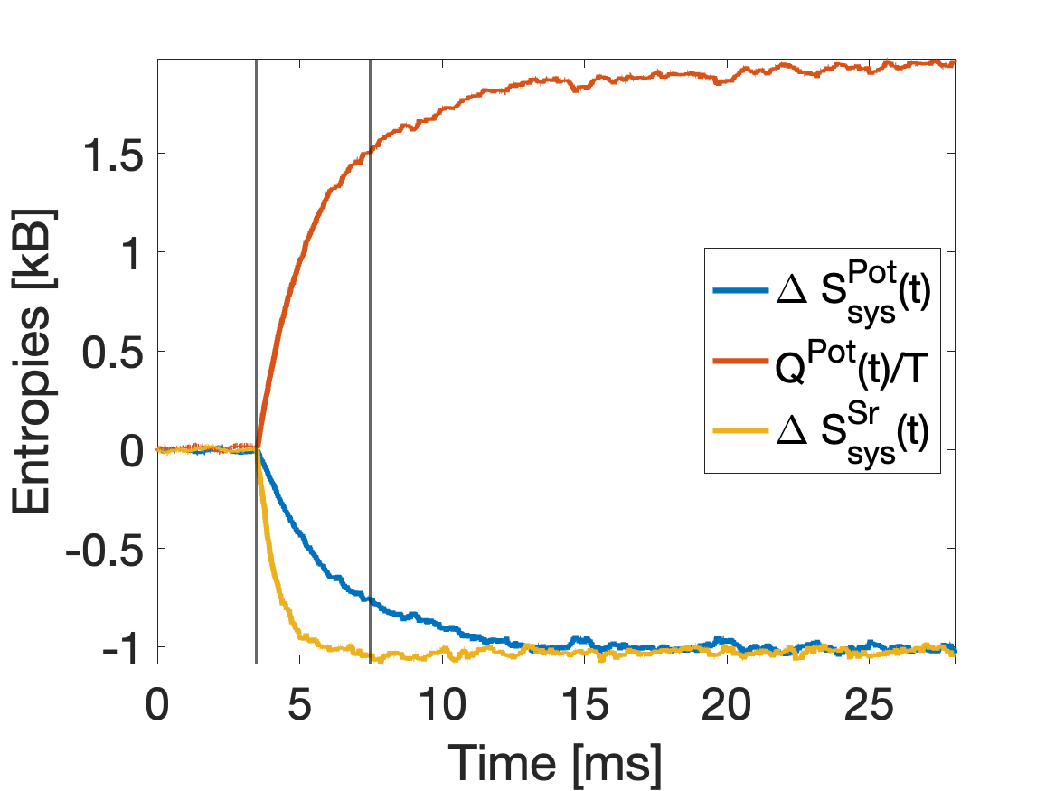
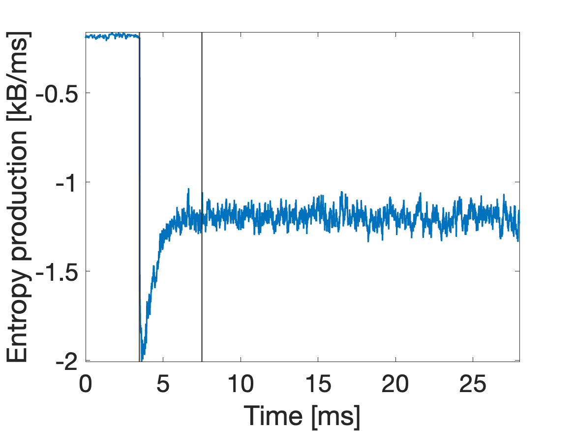
Figure 6: (Top) Total cumulative ensemble-averaged heat (red line) and ensemble-averaged system entropy (blue line) produced during the Eq.-to-Eq. potential quench. Ensemble-averaged cumulative system entropy for the SR-induced protocol (yellow line). As expected, both system’s entropy net production coincide. (Bottom) Resetting entropy production $\dot{S}_{\rm rst}$ as a function of time. The black vertical lines corresponds to the duration of the protocol when resetting is used.

Finally, the measure of the entropic cost of the proposed accelerated protocol proceeds in comparing minus the integrated resetting entropy production rate $-\int_{0}^{\tau{\rm sr}}\dot{S}_{\rm rst}^{\rm Sr}dt=5.3~{}\rm{k_{B}}$ to the heat dissipated by the standard potential quench $\Delta Q^{\rm pot}/T=(Q^{\rm eq}(t_{f})-Q^{\rm pot}(t_{i}))T=1.96~{}\rm{k_{B}}$.

Comparison with known optimal techniques in harmonic potentials - In the case of harmonic external potentials $V(x)=\kappa x^{2}/2$, SST methods exist [5] and the full characterization of the energetics associated allowed the derivation of optimal protocols [14] were the dissipated work (and heat) is minimized for a given acceleration with respect to thermal relaxation. Here we propose to compare the entropic cost of the SR-induced acceleration to the entropy generated by an optimal protocol imposing the same 8-fold increase of the control parameter and leading to the same 3.25 acceleration. This physical meaning comparison is of course limited since the optimal protocol applies on a harmonic potential and while we work with linear v-shaped potential. However, the fact that we obtain very similar cost is a promising result for the generalization of SR-induced acceleration.

Two states defined respectively by $\kappa_{i}$ and $\kappa_{f}$ are characterized by a free-energy difference $\Delta F=k_{B}T\rm{ln}\sqrt{\kappa_{f}/\kappa_{i}}$. For a step-like change of stiffness from $\kappa_{i}$ to $\kappa_{f}$ the work reads $\Delta W^{\rm ho,step}=k_{B}T(\kappa_{f}-\kappa_{i})/(2\kappa_{i})$. For an optimal protocol imposing an n-fold acceleration $\Delta t\equiv\tau_{r}/n$, the work reads $\Delta W^{\rm ho,opt}=\gamma(\sqrt{k_{B}T/\kappa_{i}}-\sqrt{k_{B}T/\kappa_{f}})^{2}/(2\Delta t)+\Delta F$ as detailed in [14]. The total entropic cost in both cases reads $\Delta S_{\rm tot}{\rm ho}=(W^{\rm ho}-\Delta F)/T$ which corresponds to the dissipated work devided by the temperature. Feeding in $\kappa_{f}=8\times\kappa_{i}$ and $\Delta t=\tau_{r}/3.5$ to stick to the conditions of the protocol studied here, on obtains $\Delta S_{\rm tot}^{\rm ho,step}=2.16~{}\rm{k_{B}}$ and $\Delta S_{\rm tot}^{\rm ho,opt}=10.64~{}\rm{k_{B}}$. Those numbers are close to the obtained results for the v-shaped step-like potential quench $\Delta S_{\rm tot}^{\rm eq}=2.96~{}\rm{k_{B}}$ and for the SR-induced protocol $\Delta S_{\rm tot}^{\rm Sr}=6.3~{}\rm{k_{B}}$.

Appendix B Appendix B: Transient probability density for SR

Starting with initial conditions $x(0)=0$, a free Brownian particle undergoing SR will evolve towards a non-equilibrium steady-state $P_{s}(x)$. In the transient, its time dependant PDF $\rho(x,t)$ follows a non trivial evolution [31]. The PDF splits into two region, a central region where it already takes the form of the long-time steady state and an outer region showing the Gaussian growth of a free Brownian object. The boundary between both profiles grows linearly in time and since it shows a second-order discontinuity, it is understood as a dynamical phase transition [31].

In our case, we follow the evolution from an initial steady-state different from a $\delta$-distribution. We make the hypothesis that the PDF similarly splits into two region: an inner region reaches the final steady states, while the outer region still follows the initial profile. Both region being separated by a boundary $x_{0}(t)$ which evolves in time. More precisely, the initial steady state is $P_{i}(x)=\frac{\alpha(t_{i})}{2}e^{-\alpha(t_{i})|x|}$ where $\alpha(t_{i})=\sqrt{\lambda(t_{i})/D}$ and the final state is $P_{f}(x)=\frac{\alpha(t_{f})}{2}e^{-\alpha(t_{f})|x|}$ where $\alpha(t_{f})=\sqrt{\lambda(t_{f})/D}$. We define a window-function $W(x,t)=W[x_{0}(t)]=1$ for $x\in[-x_{0}(t),x_{0}(t)]$ and $=0$ elsewhere, its complementary function is defined as $\bar{W}\equiv 1-W$. The expected PDF then reads

$$f(x,t)=W[x_{0}(t)]P_{i}(x)+e^{-(\alpha(t_{f})-\alpha(t_{i}))|x_{0}(t)|}\bar{W}[X_{0}(t)]P_{f}(t)$$ (15)

where $\mathcal{Z}$ is a time-dependant normalization. The time-dependant boundary $x_{0}(t)$ evolves from zero (then $f(x,0)=P_{i}(x)$) to infinity (then $f(x,\infty)=P_{f}(x)$.

In other words, the PDF follow $f(x,t)\sim e^{-tI(x/t)}$ where $I(s)$ is the large deviation function, or rate function. In the inner region $|s|<x_{0}(t)$ we have $I(s)=\alpha(t_{f})s$ and for the outer region $|s|>x_{0}(t)$, we have $I(s)=\alpha(t_{i})s+(\alpha_{f}-\alpha_{i})x_{0}(t)$.

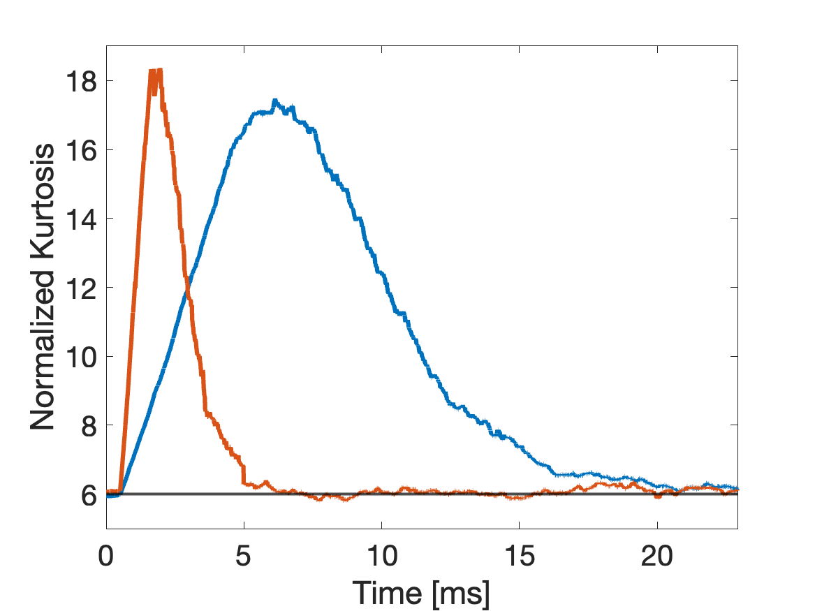
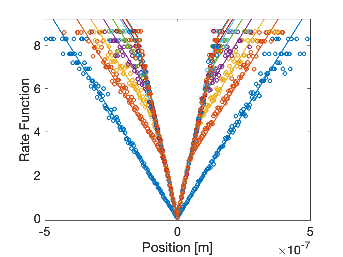
Figure 7: (Top) Time-dependant kurtosis (fourth cumulent) of an ensemble of $10^{5}$ particles undergoing an 8-flod increase in potential slope (blue line) or resetting rate (red line). The deviation from the initial and final value of six shows the departure from a simple Laplace-profile. (Bottom) Log of PDFs through time $I(x)=\rm{ln}(\rho(x,t))-\rm{ln}(\mathcal{Z}(t))$ together with the fitted piece-wise linear function.

On Fig. 7 (Top) we show the measured normalized Kurtosis $k=\langle x-\langle x\rangle\rangle^{4}/\langle x^{2}\rangle^{2}$ on an ensemble of trajectories $x_{t}$ undergoing the same 8-fold quench as in the main text. The sharp increase from the standard value $k=6$ defining a Laplace distribution reveals the non-trivial shape of the PDF during the transient.

On Fig. 7 (Bottom) we show the rate function’s evolution in time (colored circles) together with a fit using the above $I(s)$, where the only fitting parameter is the boundary $x_{0}(t)$. We clearly see how the rate function evolves from the initial linear profile (blue circles) towards a piece wise-constant intermediate regime. It eventually reaches the final steady-state linear profile for large times. On Fig. 8 (Top) we show some PDF during the transient both for a potential quench (blue circles) and for a SR $\lambda$-quench (red triangles). We superimpose $f(x,t)$ as defined Eq. (15) fed with the time-dependant value of $x_{0}(t)$ obtained from the rate function fits.

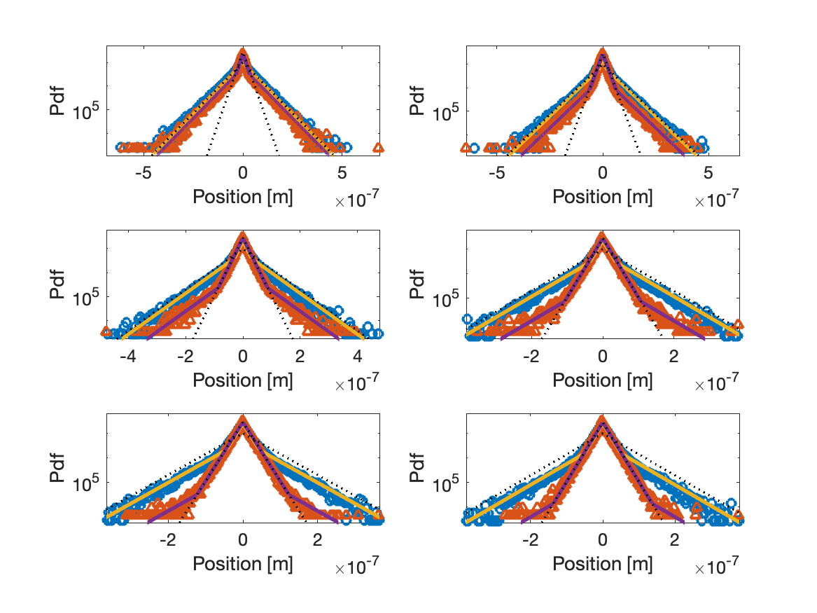
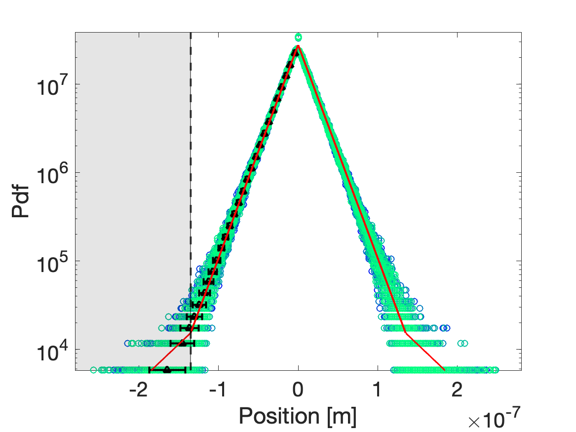
Figure 8: (Top) Some probability densities $\rho(x,t)$ during the transient, under a potential quench (blue circles) or a SR $\lambda$-quench (red triangles) together with the expected densities $f(x,t)$ using the single fitting parameter extracted from the rate function fits. (Bottom) a thousand consecutive measured PDF on an ensemble on $10^{5}$ trajectories in final steady-state (blue to green), average and standard deviation of the measured position at a given value $P_{f}(x)$ (black triangle) and transient $f(x,t)$ defined by $x_{0}(t)=1.3\times 10^{-7}$.

The time-dependence of $x_{0}(t)$ is shown on Fig. 3 of the main text. Importantly, the numerically measured values of $x_{0}(t)$ only keeps a physical significance in a defined range as we show here. On Fig. 8 (Bottom) we show the dispersion in numerical histogram’s tails. This will lead to an upper bound on the measurable values of $x_{0}$ Indeed, $x_{0}$ is extracted from the fitting of Eq. (15) on the rate function. As seen here with the red line, $f(x,t)$ defined by $x_{0}(t)=1.3\times 10^{-7}$ falls into the errobars on the estimation of $x$ until the tail of the histogram. Any larger value of $x_{0}(t)$ will also fall within the same standard deviation. We therefore use this value of $x_{0}(t)=1.3\times 10^{-7}$ as an upper bound set by numerical precision (it corresponds to the limit of the $x_{0}(t)$ plot the main text).

Appendix C Appendix C: Finite-time resetting

If each resetting event takes a finite time, then it needs to be compared to the acceleration gained with respect to the potential quench protocol. More precisely, finite-time SR stays beneficial only if the accelerated relaxation time $\tau_{\rm{SR}}$ plus the time needed for each resetting events is still smaller than $\tau_{r}$. For a resetting rate $\lambda$, we can define $N\equiv\lambda*\tau_{\rm{SR}}$ as the average number of resetting events needed during the transient. Having in mind the protocol presented in the paper, this corresponds to the minimal (average) number of resetting to accelerate a transition between equilibrium states. If each resetting events takes a time $t$, the finite-time SR stays beneficial as long as $\tau_{\rm{SR}}+Nt\leq\tau_{r}$ which allow to define a critical maximal time per resetting events

$$t_{c}=\frac{1}{\lambda}\left(\frac{\tau_{r}}{\tau_{\rm{SR}}}-1\right)$$ (16)

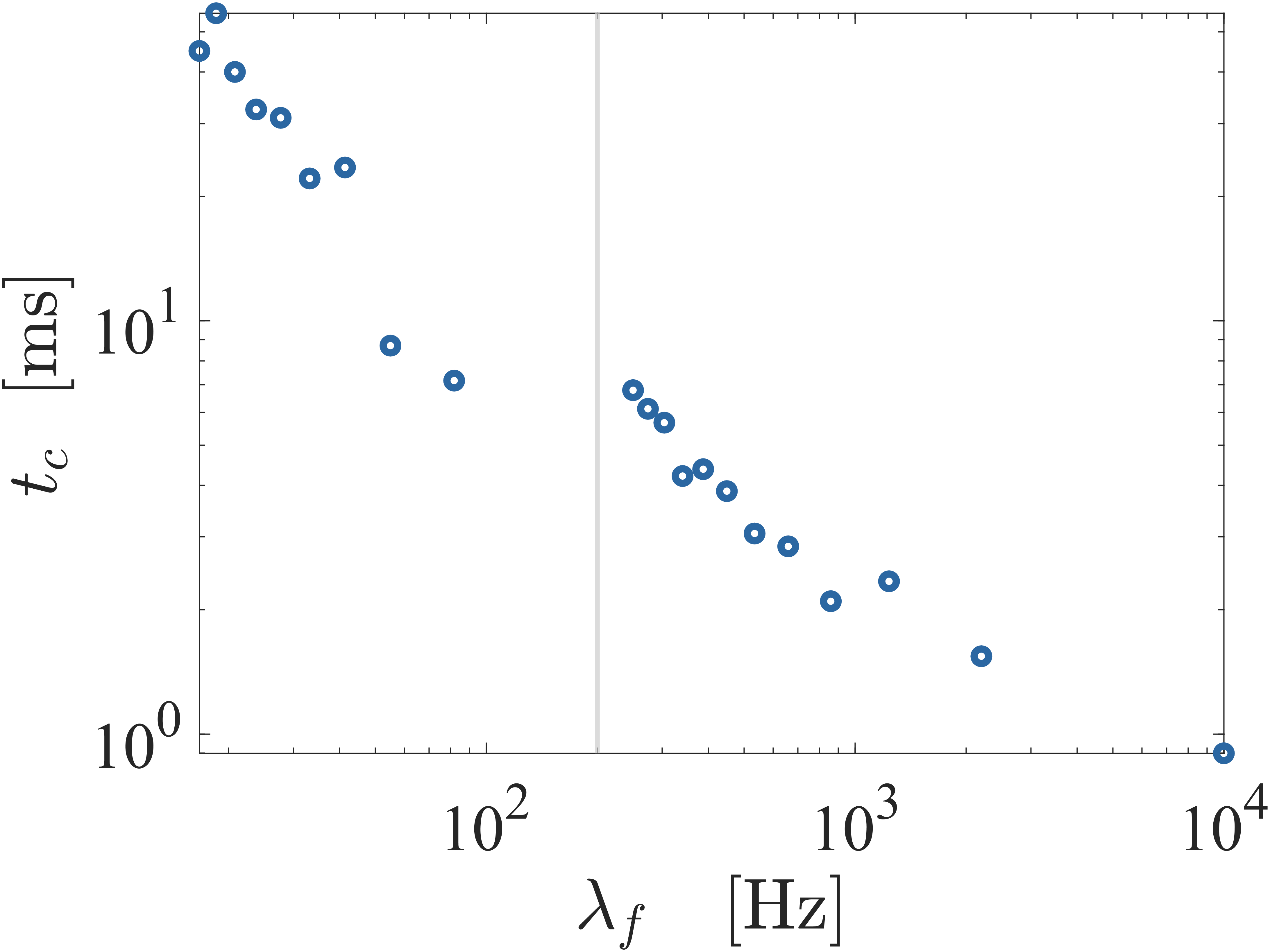
Figure 9: Maximal time (in milliseconds) allowed per resetting event to still obtain a net acceleration with respect to a potential quench. It is plotted as a function of the final resetting rate $\lambda_{f}$ with constant $\lambda_{i}=200$ Hz.

On Fig. 9 we plot the critical time $t_{c}$ as a function of the final resetting rate, with constant initial $\lambda_{i}=200$ Hz. $t_{c}$ ranges from hundreds of milliseconds for small $\lambda_{f}$ (i.e. for large decompression with very long relaxation rates) down to a millisecond for large $\lambda_{f}$ (i.e. strong compression with very short relaxation time). On all this range, the experimental feasibility of such acceleration is clear. Indeed, by inducing resetting via intermittent strong optical traps, the relaxation times implied and hence the time needed for each resetting event can be shorter than a millisecond [20].

References

- Patra and Jarzynski [2017] A. Patra and C. Jarzynski, Shortcuts to adiabaticity using flow fields, New Journal of Physics 19, 125009 (2017), publisher: IOP Publishing.
- Guéry-Odelin et al. [2019] D. Guéry-Odelin, A. Ruschhaupt, A. Kiely, E. Torrontegui, S. Martínez-Garaot, and J. Muga, Shortcuts to adiabaticity: Concepts, methods, and applications, Reviews of Modern Physics 91, 045001 (2019), publisher: American Physical Society.
- Plata et al. [2021] C. A. Plata, A. Prados, E. Trizac, and D. Guéry-Odelin, Taming the time evolution in overdamped systems: Shortcuts elaborated from fast-forward and time-reversed protocols, Phys. Rev. Lett. 127, 190605 (2021).
- Guéry-Odelin et al. [2023] D. Guéry-Odelin, C. Jarzynski, C. A. Plata, A. Prados, and E. Trizac, Driving rapidly while remaining in control: classical shortcuts from Hamiltonian to stochastic dynamics, Reports on Progress in Physics 86, 035902 (2023), publisher: IOP Publishing.
- Martínez et al. [2016] I. A. Martínez, A. Petrosyan, D. Guéry-Odelin, E. Trizac, and S. Ciliberto, Engineered swift equilibration of a Brownian particle, Nature Physics 12, 843 (2016), number: 9 Publisher: Nature Publishing Group.
- Chupeau et al. [2018] M. Chupeau, B. Besga, D. Guéry-Odelin, E. Trizac, A. Petrosyan, and S. Ciliberto, Thermal bath engineering for swift equilibration, Phys. Rev. E 98, 010104 (2018).
- Raynal et al. [2023] D. Raynal, T. de Guillebon, D. Guéry-Odelin, E. Trizac, J.-S. Lauret, and L. Rondin, Shortcuts to equilibrium with a levitated particle in the underdamped regime, Phys. Rev. Lett. 131, 087101 (2023).
- Baldassarri et al. [2020] A. Baldassarri, A. Puglisi, and L. Sesta, Engineered swift equilibration of a Brownian gyrator, Physical Review E 102, 030105 (2020), publisher: American Physical Society.
- Prados [2021] A. Prados, Optimizing the relaxation route with optimal control, Phys. Rev. Res. 3, 023128 (2021).
- Sekimoto [1998] K. Sekimoto, Langevin Equation and Thermodynamics, Progress of Theoretical Physics Supplement 130, 17 (1998), https://academic.oup.com/ptps/article-pdf/doi/10.1143/PTPS.130.17/5213518/130-17.pdf .
- Seifert [2012] U. Seifert, Stochastic thermodynamics, fluctuation theorems and molecular machines, Reports on progress in physics 75, 126001 (2012).
- Schmiedl and Seifert [2007] T. Schmiedl and U. Seifert, Optimal finite-time processes in stochastic thermodynamics, Phys. Rev. Lett. 98, 108301 (2007).
- Zhang [2020] Y. Zhang, Work needed to drive a thermodynamic system between two distributions, Europhysics Letters 128, 30002 (2020), publisher: EDP Sciences, IOP Publishing and Società Italiana di Fisica.
- Rosales-Cabara et al. [2020] Y. Rosales-Cabara, G. Manfredi, G. Schnoering, P.-A. Hervieux, L. Mertz, and C. Genet, Optimal protocols and universal time-energy bound in brownian thermodynamics, Phys. Rev. Res. 2, 012012 (2020).
- Pires et al. [2023] L. B. Pires, R. Goerlich, A. L. da Fonseca, M. Debiossac, P.-A. Hervieux, G. Manfredi, and C. Genet, Optimal time-entropy bounds and speed limits for brownian thermal shortcuts, Phys. Rev. Lett. 131, 097101 (2023).
- Evans and Majumdar [2011a] M. R. Evans and S. N. Majumdar, Diffusion with Stochastic Resetting, Physical Review Letters 106, 160601 (2011a).
- Evans et al. [2020] M. R. Evans, S. N. Majumdar, and G. Schehr, Stochastic Resetting and Applications, Journal of Physics A: Mathematical and Theoretical (2020), publisher: IOP Publishing.
- Tal-Friedman et al. [2020] O. Tal-Friedman, A. Pal, A. Sekhon, S. Reuveni, and Y. Roichman, Experimental realization of diffusion with stochastic resetting, The journal of physical chemistry letters 11, 7350 (2020).
- Besga et al. [2020] B. Besga, A. Bovon, A. Petrosyan, S. N. Majumdar, and S. Ciliberto, Optimal mean first-passage time for a brownian searcher subjected to resetting: experimental and theoretical results, Physical Review Research 2, 032029 (2020).
- Goerlich et al. [2023] R. Goerlich, M. Li, L. B. Pires, P.-A. Hervieux, G. Manfredi, and C. Genet, Experimental test of landauer’s principle for stochastic resetting, arXiv preprint arXiv:2306.09503 (2023).
- Evans and Majumdar [2011b] M. R. Evans and S. N. Majumdar, Diffusion with optimal resetting, Journal of Physics A: Mathematical and Theoretical 44, 435001 (2011b).
- Evans et al. [2013] M. R. Evans, S. N. Majumdar, and K. Mallick, Optimal diffusive search: nonequilibrium resetting versus equilibrium dynamics, Journal of Physics A: Mathematical and Theoretical 46, 185001 (2013).
- Pal and Reuveni [2017] A. Pal and S. Reuveni, First passage under restart, Physical review letters 118, 030603 (2017).
- Chechkin and Sokolov [2018] A. Chechkin and I. Sokolov, Random search with resetting: a unified renewal approach, Physical review letters 121, 050601 (2018).
- Blumer et al. [2022] O. Blumer, S. Reuveni, and B. Hirshberg, Stochastic resetting for enhanced sampling, The journal of physical chemistry letters 13, 11230 (2022).
- Gupta and Jayannavar [2022] S. Gupta and A. M. Jayannavar, Stochastic resetting: A (very) brief review, Frontiers in Physics 10, 789097 (2022).
- Sokolov [2023] I. M. Sokolov, Linear response and fluctuation-dissipation relations for brownian motion under resetting, Physical Review Letters 130, 067101 (2023).
- Fuchs et al. [2016] J. Fuchs, S. Goldt, and U. Seifert, Stochastic thermodynamics of resetting, EPL (Europhysics Letters) 113, 60009 (2016), arXiv:1603.01141 [cond-mat].
- Mori et al. [2023] F. Mori, K. S. Olsen, and S. Krishnamurthy, Entropy production of resetting processes, Physical Review Research 5, 023103 (2023).
- Roldán and Gupta [2017] E. Roldán and S. Gupta, Path-integral formalism for stochastic resetting: Exactly solved examples and shortcuts to confinement, Phys. Rev. E 96, 022130 (2017).
- Majumdar et al. [2015] S. N. Majumdar, S. Sabhapandit, and G. Schehr, Dynamical transition in the temporal relaxation of stochastic processes under resetting, Phys. Rev. E 91, 052131 (2015).
- [32] See supplementary materials for additional details.
- Seifert [2005] U. Seifert, Entropy production along a stochastic trajectory and an integral fluctuation theorem, Physical review letters 95, 040602 (2005).
- Pal and Rahav [2017] A. Pal and S. Rahav, Integral fluctuation theorems for stochastic resetting systems, Physical Review E 96, 062135 (2017).
- Gupta et al. [2020a] D. Gupta, C. A. Plata, and A. Pal, Work fluctuations and jarzynski equality in stochastic resetting, Physical review letters 124, 110608 (2020a).
- Pal et al. [2021] A. Pal, S. Reuveni, and S. Rahav, Thermodynamic uncertainty relation for systems with unidirectional transitions, Physical Review Research 3, 013273 (2021).
- Gupta et al. [2020b] D. Gupta, C. A. Plata, A. Kundu, and A. Pal, Stochastic resetting with stochastic returns using external trap, Journal of Physics A: Mathematical and Theoretical 54, 025003 (2020b).
- Bodrova and Sokolov [2020] A. S. Bodrova and I. M. Sokolov, Resetting processes with noninstantaneous return, Physical Review E 101, 052130 (2020).
- Gupta et al. [2021] D. Gupta, A. Pal, and A. Kundu, Resetting with stochastic return through linear confining potential, Journal of Statistical Mechanics: Theory and Experiment 2021, 043202 (2021).
- Olsen et al. [2023] K. S. Olsen, D. Gupta, F. Mori, and S. Krishnamurthy, Thermodynamic cost of finite-time stochastic resetting, arXiv preprint arXiv:2310.11267 (2023).
- Tal-Friedman et al. [2022] O. Tal-Friedman, Y. Roichman, and S. Reuveni, Diffusion with partial resetting, Physical Review E 106, 054116 (2022).
- Lahiri and Gupta [2023] S. Lahiri and S. Gupta, Can stochastic resetting render a heat engine more efficient? 10.48550/arXiv.2308.15212 (2023), arXiv:2308.15212 [cond-mat].
- Blickle and Bechinger [2012] V. Blickle and C. Bechinger, Realization of a micrometre-sized stochastic heat engine, Nature Physics 8, 143 (2012).
- Martínez et al. [2016] I. A. Martínez, É. Roldán, L. Dinis, D. Petrov, J. M. Parrondo, and R. A. Rica, Brownian carnot engine, Nature physics 12, 67 (2016).
- Martínez et al. [2017] I. A. Martínez, É. Roldán, L. Dinis, and R. A. Rica, Colloidal heat engines: a review, Soft matter 13, 22 (2017).