SymbolNet: Neural Symbolic Regression with Adaptive Dynamic Pruning

Abstract

Contrary to the use of genetic programming, the neural network approach to symbolic regression can scale well with high input dimension and leverage gradient methods for faster equation searching. Common ways of constraining expression complexity have relied on multistage pruning methods with fine-tuning, but these often lead to significant performance loss. In this work, we propose SymbolNet, a neural network approach to symbolic regression in a novel framework that enables dynamic pruning of model weights, input features, and mathematical operators in a single training, where both training loss and expression complexity are optimized simultaneously. We introduce a sparsity regularization term per pruning type, which can adaptively adjust its own strength and lead to convergence to a target sparsity level. In contrast to most existing symbolic regression methods that cannot efficiently handle datasets with more than $O(10)$ inputs, we demonstrate the effectiveness of our model on the LHC jet tagging task (16 inputs), MNIST (784 inputs), and SVHN (3072 inputs).

I Introduction

Symbolic regression (SR) is a supervised learning method that searches for analytic expressions that best fit the data. Unlike traditional regression methods such as linear and polynomial regression, SR can fit a much wider range of complex datasets since it does not require a pre-specified functional form, which itself is dynamically evolving in the fit. Embedding in symbolic forms facilitates human interpretation of the data so that one can potentially infer the underlying principle governing the observed system, as opposed to black-box deep-learning (DL) models. For example, Max Planck in 1900 empirically fitted a formula to the data of black-body radiation spectrum [1], known as Planck’s law; this symbolically fitted function inspired the physical derivation of the law and later led to the revolutionary development of quantum theory. On the other hand, because of its compact representation compared to most DL models, SR can also serve as a distillation method for model compression, which can be used to speed up inference time and reduce computational costs in resource-constrained environments. A major downside of SR is that it is a complex combinatorial problem, as the search space for equations grows exponentially with the number of its building blocks (i.e., variables, mathematical operators, and constants), and finding the best possible candidate has been shown to be NP-hard [2].

Genetic programming (GP) has been the main approach to SR, which involves constructing an expression in a tree structure. The bottommost nodes of the tree are made up of constants and variables, while the nodes above them represent mathematical operations. It grows an expression tree in a way that mimics biological evolution, where node mutation and subtree crossover can take place to explore variations in expressions. Expression candidates are grouped into generations and take part in a tournament selection process, where individuals with the highest fitness score can survive and proceed to the next round. Despite their success in discovering human-interpretable solutions for most low-dimensional problems, these techniques are not suitable for large and high-dimensional datasets because of their discrete combinatorial approach and long search time.

Alternatively, SR can be realized in the DL framework, for example, by training a neural network (NN) with activation functions generalized to broader mathematical operations such as unary $(\cdot$)² and sin($\cdot$), as well as binary $+$ and $\times$. The NN is trained while enforcing sparse connections so that the final expressions unrolled from the NN are compact enough to be human-interpretable or efficiently deployable in a resource-constrained environment. Apart from being able to leverage faster gradient-based optimization, the searching process can also be implemented on GPUs to accelerate both training and inference, while GP-based algorithms are limited to CPUs. The key ingredient in training an NN that produces reasonable SR results with a good balance between model performance and complexity is sparsity control. However, most recent developments in the use of NN for SR have relied on less efficient pruning methods to meet the demand for sparsity, which require multiple training phases with a hard-threshold pruning followed by fine-tuning. These multistage frameworks often lead to significant performance compromise, as accuracy and sparsity are optimized in separate training phases. The absence of an effective integration of a sparsity control scheme prevents DL approaches from taking full advantage of their potential to enable SR to be applied to a wider range of problems.

In this contribution, we introduce SymbolNet, a DL approach to SR using NN in a novel and SR-dedicated pruning framework with the following properties:

• End-to-end single-phase dynamic pruning. There is only one training phase needed without fine-tuning. It does not require a pre-specified threshold to perform a “heavy-hammer-style” pruning, as, inspired by dynamic sparse training [4], there is a trainable threshold associated with each neuron, and the pruning of a neuron is automatically determined from the dynamical competition between the weight and its threshold. This pruning mechanism is extended to prune input features, so feature selection is automated as part of the framework without relying on external packages or requiring additional steps. Similarly, operator pruning is introduced, which involves dynamically transforming complex mathematical operators to basic arithmetic operations.

• Convergence to the desired sparsity levels. Sparsity is controlled by a regularization term that can adaptively adjust its relative strength during training and lead to convergence to the desired sparsity level per pruning type.

• Scalability of SR to high-dimensional datasets. Dynamic pruning can drive strong sparsity that is optimized simultaneously with model performance, allowing optimal and compact expressions to be generated to fit large and complex datasets.

As far as we are aware, most of the SR literature tested their methods primarily on datasets with input dimensions below $O(10)$, yet they have not been demonstrated to scale efficiently to high-dimensional problems such as MNIST and beyond. We test our framework to learn compact expressions from datasets with input dimensions ranging from $O(10)$ to $O(1000)$.

II Related work

Approaches to SR have traditionally been based on GP, which was first formulated in [5], arising from the question of whether it is possible to create a program that allows a computer to solve a problem in a manner similar to natural selection and genetic evolution. Eureqa [6] is one of the first GP-based SR libraries, but it was developed as a commercial proprietary, limiting its use cases in the scientific domain. PySR [7] is an open-source library recently developed by leveraging the classic GP approach, it improves with a novel evolve-simplify-optimize loop, built for practical SR and automatic discovery of scientific equations [8, 9, 10, 11, 12, 13, 14]. Other examples include gplearn [15], Operon [16], and GP-GOMEA [17].

DL has been successful in tackling complex problems in domains such as computer vision and natural language, yet until recently it has not been thoroughly investigated in the SR domain. Equation learner (EQL) [18, 19, 20] is one of the first NN architectures proposed to perform SR. The idea is to construct an NN using primitive mathematical operations for neuron activation, train to a sparse structure, and then unroll to obtain the final expression. A three-stage training scheme is used to prevent overly complex equations. First, a fully-connected NN is trained without regularization, with the regression error being the only objective so that parameters can freely vary and reach a reasonable starting point. Then in the next training phase, a $L_{1}$ regularization is imposed to encourage small weights, and a sparse connection pattern starts to emerge. Finally, all weights with magnitude below a small threshold are set to zero and frozen afterwards, equivalent to enforcing a fixed $L_{0}$ norm, and the remaining weights are fine-tuned without any regularization. Later, it has been shown that using the $L_{0.5}^{*}$ regularizer [21, 22], which is constructed from a piecewise function and serves as a smooth variant of $L_{0.5}$, can enforce stronger sparsity than $L_{1}$. These methods were demonstrated using simple dynamic system problems with input dimensions of $O(1)$.

Other variants of NN-based approaches include OccamNet [23], which uses an NN to define a probability distribution over a function space, optimized by a two-step method that first samples the functions and then updates the weights so that the probability mass is more likely to produce better fitting functions. Sparsity is maximized by introducing temperature-controlled softmax layers for sampling sparse paths through the NN. DSR [24] uses an autoregressive recurrent NN to generate expressions sequentially and optimizes based on reinforcement learning. MathONet [25] is a Bayesian learning framework that incorporates sparsity as priors and is applied to solve differential equations. N4SR [26] is a multistage learning framework that allows incorporating domain-specific prior knowledge. Another class of approaches uses a transformer pre-trained on large-scale synthetic examples to generate symbolic expressions from data; we refer the interested reader to [27, 28, 29, 30].

However, these approaches focus primarily on small and low-dimensional datasets and do not investigate how to extend scalability. GP-based methods are intrinsically hard to scale due to their discrete search strategy, while DL-based methods lack an efficient and SR-dedicated way to constrain the model size. Our method, presented in the following section, attempts to bridge this gap.

III SymbolNet architecture

In this section, we detail the model architecture and training framework. We construct an NN composed of symbolic layers with generic mathematical operators as activation functions. We introduce trainable thresholds for dynamically pruning model weights, input features, and operators, respectively. A self-adaptive regularization term is introduced for each pruning type for convergence to a target sparsity level.

III-A Neural symbolic regression

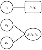
Figure 1: A symbolic layer consisting of three linear transformation nodes $z$ activated by a unary operator $f$ and a binary operator $g$.

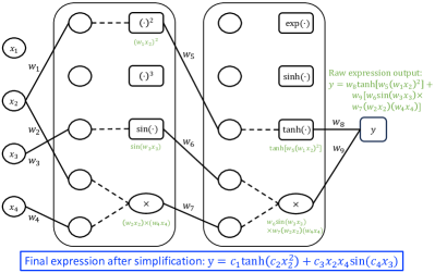
Figure 2: An example NN with four input features ($x$), two symbolic layers (big rectangles), and one output node ($y$). Each symbolic layer has five linear transformation nodes (empty circles), followed by three unary nodes (small rectangles) and one binary node (ovals). The solid lines represent node connection with nonzero weights ($w$) for the linear transformation while the dashed lines represent node activation by mathematical operations. The intermediate expression outputs (texts in green) are shown next to the nodes, whenever they are not pruned. The final expression (texts in blue) from this example model, after simplifying the constants from $w$ to $c$, is: $\bm{y=c_{1}\tanh(c_{2}x_{2}^{2})+c_{3}x_{2}x_{4}\sin(c_{4}x_{3})}$, which is compact due to the sparse connection structure. This illustrates the basic architecture of SymbolNet before incorporating the additional components for adaptive dynamic pruning.

We adopt the EQL architecture introduced in [18] to approach SR using NN, as our baseline. This architecture is no different from a multilayer perceptron, except that each hidden layer is generalized to a symbolic layer composed of two operations: the usual linear transformation of outputs from the previous layer, followed by a layer of heterogeneous unary ($f(x)$: $\mathbb{R}\rightarrow\mathbb{R}$, e.g., $x^{2}$, $\sin(x)$ and $\exp(-(x)^{2})$) and binary ($g(x,y)$: $\mathbb{R}^{2}\rightarrow\mathbb{R}$, e.g., $x+y$, $xy$, and $\sin(x)\cos(y)$) operations as activation functions. Therefore, if there are $u$ unary operators and $b$ binary operators in a symbolic layer, then its input dimension is $u+2b$ and its output dimension is $u+b$. An example is illustrated in Fig. 1, where $u=1$ and $b=1$.

III-B Dynamic pruning per network component type

The expressiveness of NNs is partially attributed to the vast number of adjustable parameters they possess. Even a shallow NN can be over-parameterized in the sense of symbolic representation, so controlling sparsity is a critical factor for NN-based SR, while ensuring the model performance is reasonably maintained. An example of a sparsely connected NN composed of symbolic layers that generates a compact expression is illustrated in Fig. 2.

The dynamic sparse training was introduced in [4]. Instead of fixing a single pruning threshold for all weights and applying a “heavy-hammer-style” pruning, the method defines a threshold vector for each layer, while the thresholds are trainable and can be updated through backpropagation. The pruning is therefore a dynamic process, where the weights and their associated thresholds are continuously competing, and the pruning is more fine-grained as it happens at each training step rather than between epochs. Since both a weight and its threshold continue to update even after the weight is pruned, it is possible to recover a pruned weight when the competition reverses. It is a single training schedule that does not require multistage training with fine-tuning, and the model parameters and sparsity are optimized simultaneously. This simple yet powerful framework will be of particular interest for NN-based SR. Inspired by that, we adopt it for our model to perform a neuron-wise weight pruning, then we generalize the idea to prune input features and mathematical operators as well.

To apply dynamic pruning, Ref. [4] used a step function as a masking function, and a piecewise polynomial estimator, which is nonzero and finite in the range $[-1,1]$ but zero elsewhere, to approximate its derivative in the backward pass to prevent a zero gradient in the thresholds, since its original derivative is almost zero everywhere. In this work, we employ a similar binary step function $\theta(x)=\mathbf{1}_{x>0}$ (i.e., 1 if $x>0$, otherwise 0) for masking in the forward pass, but with a smoother estimator in the backward pass using the derivative of the sigmoid function $\frac{d\theta(x)}{dx}\approx\frac{\kappa e^{-\kappa x}}{(1+e^{-\kappa x})^{2}}$with $\kappa=5$, which is nonzero everywhere.

We introduce a pruning mechanism respectively for model weights, input features, unary nodes, and binary nodes, as illustrated in Fig. 3 and explained in the following subsections.

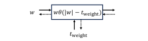
(a)

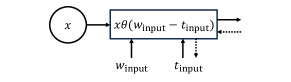
(b)

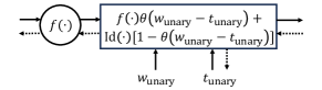
(c)

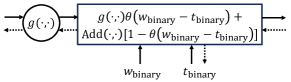
(d)

Figure 3: Schematic of the SR-dedicated dynamic pruning mechanism as part of the SymbolNet architecture: (a) model weights, (b) input features, (c) unary operators, and (d) binary operators. Solid arrows represent the forward pass, while dotted arrows represent the backward pass, connecting the trainable parameters. The SymbolNet architecture is formed by combining these elements with the basic network architecture illustrated, for example, in Fig. 2.

III-B1 Pruning of model weights

For each weight $w$, we associate it with a trainable pruning threshold $t_{\text{weight}}$. So, for each layer that performs linear transformation with input dimension $n$ and output dimension $m$, a weight matrix and a threshold matrix are present: $\bm{w},\bm{t}_{\text{weight}}\in\mathbb{R}^{n\times m+m}$, where the second $m$ is the number of bias terms. Each threshold is initialized to zero and is clipped to the range of $[0,\infty)$ during parameter updates, since the magnitude of each $w$ is not bounded. The neuron-wise pruning per layer is carried out using the step function matrix $\bm{\Theta}_{\text{weight}}=\theta(|\bm{w}|-\bm{t}_{\text{weight}})\in\mathbb{R}^{n\times m+m}$ applied to propagate $w_{ij}\rightarrow(\bm{w}\odot\bm{\Theta}_{\text{weight}})_{ij}=w_{ij}\theta(|w_{ij}|-t_{\text{weight},ij})$, as shown in Fig. 3a. Concatenating all layers of the architecture, we denote $\bm{W}=\{\bm{w}\}$ and $\bm{T}_{\text{weight}}=\{\bm{t}_{\text{weight}}\}$ with the total dimension as the total number of weights $n_{\text{weight}}$.

III-B2 Pruning of input features

Similarly, for each input node $x$, we associate it with an auxiliary weight $w_{\text{input}}$ and a trainable pruning threshold $t_{\text{input}}$. Since there is already a linear transformation of the inputs when feeding to the next layer, and that on the pruning side only the relative distance between the weight and threshold is relevant, hence a trainable auxiliary weight will be redundant, so we fix all $w_{\text{input}}=1$ and set them untrainable. Each threshold is initialized to zero and is clipped to the range of $[0,1]$ during parameter updates. For the input vector $\bm{x}\in\mathbb{R}^{n_{\text{input}}}$, there are an auxiliary weight vector and a threshold vector $\bm{W}_{\text{input}},\bm{T}_{\text{input}}\in\mathbb{R}^{n_{\text{input}}}$, the pruning operation is carried out by the step function vector $\bm{\Theta}_{\text{input}}=\theta(\bm{W}_{\text{input}}-\bm{T}_{\text{input}})$ applied to propagate $x_{i}\rightarrow(\bm{x}\odot\bm{\Theta_{\text{input}}})_{i}=x_{i}\theta(1-T_{\text{input},i})$, as shown in Fig. 3b. In other words, an input node is pruned when its associated threshold value is 1.

III-B3 Pruning of mathematical operators

We consider simplification of complex mathematical operators to basic arithmetic ones instead of pruning them to zeros directly, since such a prune-to-zero pruning can be carried out by pruning the corresponding weights in their linear transformation when propagating to the next layer.

Similar to input pruning, for each unary operator node $f(\cdot)$: $\mathbb{R}\rightarrow\mathbb{R}$, we associate it with an untrainable auxiliary weight fixed to $w_{\text{unary}}=1$ and a trainable pruning threshold $t_{\text{unary}}\in[0,1]$. The pruning operation is applied to each unary node as $f(\cdot)\rightarrow[f(\cdot)\theta(1-t_{\text{unary}})+\text{Id}(\cdot)(1-\theta(1-t_{\text{unary}}))]$, where $\text{Id}(\cdot)$ is the identity function, as shown in Fig. 3c. That is, an unary operator will be simplified to an identity operator when needed, which can help prevent overfitting and overly complicated components such as function nesting (e.g., $\sin(\sin(\cdot))$). We denote all thresholds of this type by a vector $\bm{T}_{\text{unary}}$ with a dimension of $n_{\text{unary}}$, which is the total number of unary nodes in the architecture.

Similarly, for each binary operator node $g(\cdot,\cdot)$: $\mathbb{R}^{2}\rightarrow\mathbb{R}$, we associate it with an untrainable auxiliary weight fixed to $w_{\text{binary}}=1$ and a trainable pruning threshold $t_{\text{binary}}\in[0,1]$, applying to it the pruning operation $g(\cdot,\cdot)\rightarrow[g(\cdot,\cdot)\theta(1-t_{\text{binary}})+\text{Add}(\cdot,\cdot)(1-\theta(1-t_{\text{binary}}))]$, where $\text{Add}(\cdot,\cdot)$ is the addition operator, as shown in Fig. 3d. That is, an binary operator will be simplified to an addition operator when needed. We denote all thresholds of this type by a vector $\bm{T}_{\text{binary}}$ with a dimension of $n_{\text{binary}}$, which is the total number of binary nodes in the architecture.

III-C Self-adaptive regularization for sparsity

We introduce a regularization term per threshold type for driving large threshold values. For the model weight thresholds, similar to [4], we use the form $L_{\text{threshold}}^{\text{weight}}=\frac{1}{n_{\text{weight}}}\sum_{i=1}^{n_{\text{weight}}}\exp(-T_{\text{weight},i})$, where the sum runs over all the weight thresholds in the architecture. Since each threshold $T_{\text{weight},i}\in[0,\infty)$ is unbounded, this sum of the exponential of each threshold will not drop to zero immediately if any of the thresholds becomes large. For other types with bounded thresholds, we take a more efficient form with a single exponential $L_{\text{threshold}}^{\text{aux}=\text{\{input,unary,binary\}}}=\exp(-\frac{1}{n_{\text{aux}}}\sum_{i=1}^{n_{\text{aux}}}T_{\text{aux},i})$.

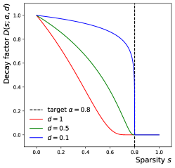
Figure 4: The decay factor, $D(s;\alpha,d)$, is used to reduce the rate of increase in thresholds when the sparsity ($s$) is approaching its target value ($\alpha$), and to stop the high-threshold driving when $s\geq\alpha$, during dynamic pruning. The profiles of $D(0\leq s\leq 1)$ for a target sparsity of $\alpha=0.8$ at three different decay rates ($d$) are shown.

For each of the regularizers, we introduce an additional decay factor:

$$D(s;\alpha,d)=\exp\bigg{[}-\bigg{(}\frac{\alpha}{\alpha-\text{min}(s,\alpha)}\bigg{)}^{d}+1\bigg{]}$$ (1)

where the sparsity $s\in[0,1]$ is the ratio of pruned parameters or nodes evaluated at each training step, $\alpha\in[0,1]$ a free parameter to set the target sparsity, and $d$ the decay rate to slow the sparsity driving. This term, when multiplied to the regularizer, effectively slows the driving of large thresholds when the sparsity $s$ grows, and eliminates the regularizer when $s\geq\alpha$. The decay factor is illustrated in Fig. 4 for different decay rates $d$.

The full regularization term for each threshold type takes the form $L_{\text{sparse}}=L_{\text{error}}D(s;\alpha,d)L_{\text{threshold}}$, where $L_{\text{error}}$ is the training loss (e.g., regression error). The strength of the threshold regularizer $L_{\text{threshold}}$ is adaptively adjusted by the product $L_{\text{error}}D(s;\alpha,d)$ which has a baseline strength set by the training loss. When the network initializes at $s=0$, the regularization is equally important as the training loss: $L_{\text{sparse}}=L_{\text{error}}$ since $L_{\text{threshold}}=D=1$. The presence of $L_{\text{threshold}}$ drives the thresholds to increase through backpropagation, which in turn decreases $L_{\text{threshold}}$. When sparsity starts to increase $s>0$, the decay factor $D$ drops below 1 to further slow the increase in thresholds. The process continues until the target sparsity is reached, where $D$ drops to 0, or a further increase in sparsity will significantly increase the training loss even when the target is not reached. Therefore, the regularizer $L_{\text{sparse}}$ is designed to drive the convergence of sparsity to a target value.

III-D Training framework

Putting all together, for a dataset $\{(\bm{x}^{i},\bm{y}^{i})\}_{i=1}^{N}$ with input $\bm{x}^{i}\in\mathbb{R}^{n_{\text{input}}}$ and label $\bm{y}^{i}\in\mathbb{R}^{n_{\text{output}}}$, the algorithm attempts to solve the following multi-objective optimization problem for a network $\phi:\mathbb{R}^{n_{\text{input}}}\rightarrow\mathbb{R}^{n_{\text{output}}}$ with output $\hat{\bm{y}}^{i}=\phi(\bm{x}^{i})$:

$$\bm{W}^{*}, \bm{T}^{*}_{\text{weight}},\bm{T}^{*}_{\text{aux}}=$$ (2)

$$\operatorname*{arg\,min}_{\bm{W},\bm{T}_{\text{weight}},\bm{T}_{\text{aux}}}\mathcal{L}(\bm{W},\bm{T}_{\text{weight}},\bm{T}_{\text{aux}};\alpha_{\text{weight}},\alpha_{\text{aux}},d),$$

where

$$\mathcal{L} =L_{\text{error}}+L_{\text{sparse}}^{\text{weight}}+L_{\text{sparse}}^{\text{aux}}$$ (3)

$$L_{\text{sparse}}^{\text{weight}} =L_{\text{error}}D(s_{\text{weight}};\alpha_{\text{weight}},d)\frac{1}{n_{\text{weight}}}\sum_{i=1}^{n_{\text{weight}}}\exp(-T_{\text{weight},i})$$

$$L_{\text{sparse}}^{\text{aux}} =L_{\text{error}}D(s_{\text{aux}};\alpha_{\text{aux}},d)\exp\bigg{(}-\frac{1}{n_{\text{aux}}}\sum_{i=1}^{n_{\text{aux}}}T_{\text{aux},i}\bigg{)},$$

with $\text{aux}=\text{\{input,\,unary,\,binary\}}$. We use, for example, the mean squared error (MSE) as the training loss: $L_{\text{MSE}}=\frac{1}{Nn_{\text{output}}}\sum_{i=1}^{N}\sum_{j=1}^{n_{\text{output}}}(y_{j}^{i}-\hat{y}_{j}^{i})^{2}$. We fix $d=0.01$ for our experiments presented in the next section. The remaining free parameters are $\alpha_{\text{weight}}$, $\alpha_{\text{input}}$, $\alpha_{\text{unary}}$, and $\alpha_{\text{binary}}$, which set the target sparsity for different types of pruning.

In this single-phase training framework, the overall sparse structure is divided into sparse substructures of the model weights, input features, unary operators, and binary operators, respectively. In particular, a set of sparse input features is automatically searched without relying on external feature selection process. Each of these sparse substructures is dynamically determined by the competition between the corresponding weights and thresholds. Moreover, the sparse structure also competes dynamically with the regression performance, so that both are optimized simultaneously. One can freely choose the target sparsity levels for convergence rather than blindly tuning some hyperparameters without physical meaning. The final symbolic expressions are obtained by unrolling the trained network.

IV Experimental setup

IV-A Expression complexity

To quantify the size of a symbolic model, we use a metric called expression complexity [7]. It is computed by counting all possible steps in traversing the expression tree, which is equivalent to the total number of nodes in the tree. For example, the expression $y=c_{1}\tanh(c_{2}x_{2}^{2})+c_{3}x_{2}x_{4}\sin(c_{4}x_{3})$ generated in Fig. 2 has a complexity of 17, and the counting is illustrated in Fig. 5. The Sympy library [31] provides the “preorder_traversal” method which can be used to calculate the number of steps needed to traverse a given expression.

We have assumed that all types of tree node (i.e., mathematical operator, input variable, and constant) have the same complexity of 1 during the counting. However, this may not be the case in general, such as in the context of Field-Programmable Gate Arrays (FPGAs) where computing $\tan(\cdot)$ requires multiple times more clock cycles than $\sin(\cdot)$. On the other hand, for example, if mathematical functions are approximated using lookup tables that all require one clock cycle to compute, then the assumption that all unary operators are equally weighted becomes valid [32]. The definition of complexity per node type depends on the implementation and the resource allocation strategy, which we do not investigate in depth and instead take the most straightforward assumption in this paper.

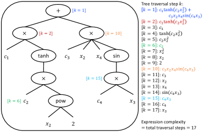
Figure 5: Counting the complexity of an expression in its tree representation by tree traversal. The expression $\bm{y=c_{1}\tanh(c_{2}x_{2}^{2})+c_{3}x_{2}x_{4}\sin(c_{4}x_{3})}$ is taken from the example NN in Fig. 2. The tree representation of this expression is shown in the square, and the sub-expressions at each step of the traversal ($k$) are listed on the right. The expression complexity of this example is 17, assuming all mathematical operators, input features, and constants are equally weighted. Note that the number of possible traversal steps is equivalent to the number of nodes in the tree.

IV-B Baseline for comparison: EQL with multistage pruning

We use the EQL architecture [18, 19, 20] trained in a three-stage pruning framework [21] as the baseline for SymbolNet to compare against. In this baseline framework, model parameters are regularized by the smoothed $L_{0.5}$ term called $L^{*}_{0.5}$, which is controlled by a free parameter $\lambda$:

$$\mathcal{L} =L_{\text{MSE}}+\lambda L_{0.5}^{*}$$ (4)

$$L_{0.5}^{*}(w) =\begin{cases}|w|^{0.5}&,|w|\geq a\\ \big{(}-\frac{w^{4}}{8a^{3}}+\frac{3w^{2}}{4a}+\frac{3a}{8}\big{)}^{0.5}&,|w|<a\end{cases}$$

where we set $a=0.01$. In the first phase, $L_{0.5}^{*}$ is turned off ($\lambda=0$) so the model can learn the regression maximally and set a good starting point for the model weights. In the second phase, $L_{0.5}^{*}$ is turned on ($\lambda>0$) to suppress the magnitudes of the weight so that a sparse model structure emerges. After that, the small-magnitude weights are set to zero and frozen afterwards. In the final phase, $L_{0.5}^{*}$ is turned off ($\lambda=0$) again when training (fine-tuning) the sparse model. In the experiments that follow, we use similar configurations, such as network sizes and operator choices, as SymbolNet, then vary $\lambda$ from $10^{-4}$ to $10^{-1}$ and the hard pruning threshold from $10^{-4}$ to $10^{-1}$, to obtain a complexity scan by running multiple trials.

IV-C Datasets and experiments

We test our framework on datasets with input dimensions ranging from $O(10)$ to $O(1000)$: the Large Hadron Collider (LHC) jet tagging dataset with 16 inputs [33], MNIST with 784 inputs [34], and SVHN with 3072 inputs [35].

IV-C1 LHC jet tagging

We chose a dataset from the field of high-energy physics due to its increasing demands for efficient machine learning solutions in resource-constrained environments such as the LHC experiments [36, 37].

In collider experiments, a jet refers to a cone-shaped object that contains a flow of particles whose origin can be traced back to the decay of an unstable particle. The process of determining the original particle from the characteristics of the jet is known as jet tagging. The LHC jet tagging dataset consists of simulated jets produced from proton-proton collision at the LHC, designed to benchmark a five-class classification task: identifying a jet originating from a light quark, gluon, W boson, Z boson, or top quark, from a list of 16 physics-motivated input features constructed from detector observables: $\big{(}$$\sum z\,\text{log}\,z$, $C_{1}^{\beta=0,1,2}$, $C_{2}^{\beta=1,2}$, $D_{2}^{\beta=1,2}$, $D_{2}^{(\alpha,\beta)=(1,1),(1,2)}$, $M_{2}^{\beta=1,2}$, $N_{2}^{\beta=1,2}$, $m_{\text{mMDT}}$, Multiplicity$\big{)}$. The dataset is publicly available in [33], and further descriptions can be found in [38, 39, 40].

The inputs are standardized and their distributions are shown in Fig. 6a.

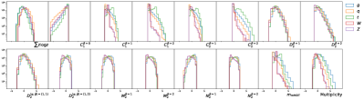
(a)

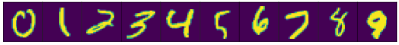
(b)

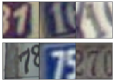
(c)

Figure 6: (a): Distributions of the 16 standardized input features in the LHC jet tagging dataset. From top left to top right: $\sum z\,\text{log}\,z$, $C_{1}^{\beta=0}$, $C_{1}^{\beta=1}$, $C_{1}^{\beta=2}$, $C_{2}^{\beta=1}$, $C_{2}^{\beta=2}$, $D_{2}^{\beta=1}$, and $D_{2}^{\beta=2}$. From bottom left to bottom right: $D_{2}^{(\alpha,\beta)=(1,1)}$, $D_{2}^{(\alpha,\beta)=(1,2)}$, $M_{2}^{\beta=1}$, $M_{2}^{\beta=2}$, $N_{2}^{\beta=1}$, $N_{2}^{\beta=2}$, $m_{\text{mMDT}}$, and Multiplicity. Five jet classes are plotted separately: gluon (blue), light quark (orange), top quark (green), W boson (red), and Z boson (purple). (b): MNIST input images with one example per class. (c): SVHN input images with three examples from the digit “1” class (top) and the digit “7” class (bottom), respectively.

The labels are one-hot encoded. We train SymbolNet with five output nodes to generate five expressions corresponding to the five jet substructure classes. We consider one or two hidden symbolic layers, with unary operators including $\sin(\cdot)$, $\cos(\cdot)$, $\exp(\cdot)$, $\exp(-(\cdot)^{2})$, $\sinh(\cdot)$, $\cosh(\cdot)$, and $\tanh(\cdot)$, and binary operators $+$ and $\times$. To obtain a range of expression complexity, we run multiple trials by varying the number of operators in ranges $u\in[2,30]$ and $b\in[2,30]$, and the target sparsity levels in ranges $\alpha_{\text{weight}}\in[0.6,0.99]$, $\alpha_{\text{input}}\in[0.4,0.9]$, $\alpha_{\text{unary}}\in[0.2,0.5]$, and $\alpha_{\text{binary}}\in[0.2,0.5]$.

IV-C2 MNIST and binary SVHN

We aim to demonstrate that SymbolNet can handle datasets with high input dimensions that most existing SR methods cannot process efficiently. To illustrate this, we examine the MNIST and SVHN datasets. The objective is not to implement an exhaustive classifier for state-of-the-art accuracy, but rather to demonstrate the ability of SymbolNet to generate simple expressions to fit high-dimensional data with reasonable discriminating power.

The MNIST dataset consists of grayscale images of handwritten digits, from “0” to “9”, each having an input dimension of $28\times 28$. The task is to classify the correct digit in a given image. Fig. 6b shows an example input image for each of the ten classes. The inputs are flattened into a 1D array and denoted $x_{0},...,x_{783}$, which are all scaled to the range of $[0,1]$. We train SymbolNet with ten output nodes to generate ten expressions corresponding to the ten digit classes. We consider one or two hidden symbolic layers, with unary operators including $\sin(\cdot)$, $\cos(\cdot)$, $\exp(-(\cdot)^{2})$, and $\tanh(\cdot)$, and binary operators $+$ and $\times$. To obtain a scan of expression complexity, we vary in different trials the number of operators in ranges $u\in[2,20]$ and $b\in[2,20]$, and the target sparsity levels in ranges $\alpha_{\text{weight}}\in[0.7,0.999]$, $\alpha_{\text{input}}\in[0.6,0.99]$, $\alpha_{\text{unary}}\in[0.2,0.5]$, and $\alpha_{\text{binary}}\in[0.2,0.5]$.

Similar to MNIST, but more challenging, SVHN is a dataset of digits with an input dimension of $32\times 32\times 3$ in RGB format, where the digits are taken from noisy real-world scenes. For simplicity, we consider the binary classification between the digits “1” and “7”. Fig. 6c shows some example input images for each of the two classes considered. The inputs are flattened into a 1D array and denoted $x_{0},...,x_{3071}$, which are all scaled to the range of $[0,1]$. In this binary setting, we label the class of digit “1” as 0 and the class of digit “7” as 1, and SymbolNet has one output node and thus generates one expression per model. We consider one hidden symbolic layer with unary operators including $\sin(\cdot)$, $\cos(\cdot)$, $\exp(-(\cdot)^{2})$, and $\tanh(\cdot)$, and binary operators $+$ and $\times$. To obtain a scan of expression complexity, we run multiple trials by varying the number of operators in ranges $u\in[2,20]$ and $b\in[2,10]$, and the target sparsity levels in ranges $\alpha_{\text{weight}}\in[0.8,0.999]$, $\alpha_{\text{input}}\in[0.8,0.999]$, $\alpha_{\text{unary}}\in[0.2,0.5]$, and $\alpha_{\text{binary}}\in[0.2,0.5]$.

IV-D FPGA resource utilization and latency

It has been shown in [32] that symbolic models can reduce the consumption of FPGA resources by orders of magnitude and require significantly lower latency compared to quantized yet unpruned NNs in the LHC jet tagging dataset. Here, we perform a similar study, but using NNs that are both strongly quantized and pruned as a conventional compression strategy for the symbolic option to compare against.

For the LHC jet tagging dataset, the baseline architecture is adopted from [38], which is a fully-connected NN, or DNN, consisting of three hidden layers of 64, 32, and 32 neurons, respectively. For the MNIST and SVHN datasets, the baseline architecture is adopted from [41], which is a convolutional NN, or CNN, consisting of three convolutional blocks of 16, 16, and 24 filters with kernel size of $3\times 3$, respectively, followed by a DNN consisting of two hidden layers of 42 and 64 neurons, respectively. These baseline architectures were chosen considering that the models are small enough to fit in a single FPGA board within limited resource budgets.

The baseline NNs are further compressed by quantization and pruning. The models are trained quantization-aware using the QKeras library [42], and pruning is performed using the Tensorflow pruning API [43]. We quantize model parameters and activation functions in all hidden layers to a fixed total bit width of 6 without an integer bit, or denoted as $\langle 6,0\rangle$. The models are pruned to a sparsity level around 90%.

Both NNs and symbolic models are converted to FPGA firmware using the hls4ml library [44, 38]. Synthesis is done with Vivado HLS (2020.1) [45], targeting a Xilinx Virtex UltraScale+ VU9P FPGA (part no.: xcvu9p-flga2577-2-e), with a clock frequency set to 200 MHz (or clock period of 5 ns). We compare FPGA resource utilization and inference latency between compressed NNs and symbolic models learned by SymbolNet.

V Results

V-A LHC jet tagging

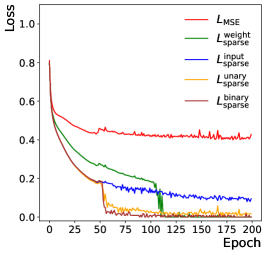
(a)

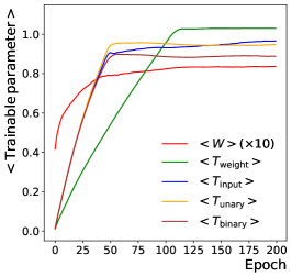
(b)

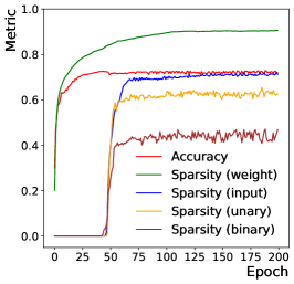
(c)

Figure 7: We demonstrate the training behavior of SymbolNet on the LHC jet tagging dataset. This SymbolNet consists of two symbolic layers, each with $u=v=20$ operations. It is trained using a batch size of 1024 with 200 epochs. Adam optimizer [46] is used with a learning rate of 0.0015. The target sparsity levels are $\alpha_{\text{weight}}=0.9$, $\alpha_{\text{input}}=0.75$, $\alpha_{\text{unary}}=0.6$, and $\alpha_{\text{binary}}=0.4$. (a): The individual loss terms in Eq. 3 as functions of the epoch. (b): The mean trainable parameters as functions of the epoch. (c): The accuracy and sparsity as functions of the epoch.

TABLE I: An example of a compact symbolic model with a mean complexity of 16 and an overall accuracy of 71% learned by SymbolNet in the LHC jet tagging dataset. Constants are rounded to 2 significant figures for the purpose of display.

Class	Expression (symbolic model for LHC jet tagging)	Complexity	AUC
$g$	$-0.041\text{Multiplicity}\times C_{1}^{\beta=1}+0.53\tanh(0.6\text{Multiplicity}-0.38C_{1}^{\beta=1})+0.24$	16	0.885
$q$	$0.073\text{Multiplicity}\times C_{1}^{\beta=1}-0.38\tanh(0.63m_{\text{mMDT}})+0.15$	12	0.827
$t$	$0.2\sin(1.2\text{Multiplicity})+0.43\sin(0.49C_{1}^{\beta=2})-0.2\tanh(0.6\text{Multiplicity}-0.38C_{1}^{\beta=1})+0.24$	24	0.915
$W$	$-0.099\sin(0.73\text{Multiplicity})+0.84\exp(-46.0(m_{\text{mMDT}}+0.14C_{1}^{\beta=1}+0.27C_{1}^{\beta=2})^{2})+0.044$	23	0.894
$Z$	$0.43\exp(-6.9(C_{1}^{\beta=2})^{2})$	8	0.851

To demonstrate the effectiveness of our adaptive dynamic pruning framework, we conducted a trial using SymbolNet with two symbolic layers, each having $u=v=20$, and set the target sparsity levels for weights, inputs, unary operators, and binary operators at $\alpha_{\text{weight}}=0.9$, $\alpha_{\text{input}}=0.75$, $\alpha_{\text{unary}}=0.6$, and $\alpha_{\text{binary}}=0.4$, respectively. The training curves for this trial are shown in Fig. 7. As seen in Fig. 7a, the training loss, $L_{\text{MSE}}$, and the other sparsity terms, $L_{\text{sparse}}$, decrease steadily until around epoch 50. At this point, the trainable thresholds for the input, unary operator, and binary operator have come close to 1 on average, as seen in Fig. 7b, so many of the nodes start to be pruned whenever their threshold is at 1. This is reflected in Fig. 7c, where the sparsity levels increase sharply, with that for the unary and binary operator reaching their target values. As a result, their losses drop steeply towards 0. However, the sparsity levels for both model weights and inputs are still some distance below their targets, so their losses are not yet close to 0. A small kink is observed in $L_{\text{MSE}}$, or accuracy, around the same time, which is caused by the steep increase in sparsity. However, the training process is dynamically adjusted, and the training loss continues to decrease as sparsity levels increase steadily. The sparsity level for model weight reaches its target around epoch 100, so its loss drops steeply there. In the end, the input sparsity is around 70%, which is below its target of 75%, so its loss does not vanish. Throughout the training, the sparsity levels converge towards their target values, with the regression and sparsity being optimized simultaneously in a dynamic process.

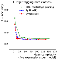
(a)

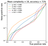
(b)

Figure 8: Performance of SymbolNet on the LHC jet tagging dataset. (a): A Pareto front is presented that illustrates the trade-off between accuracy and expression complexity when comparing the performance of SymbolNet to PySR and EQL. (b): ROC curves of a compact symbolic model with a mean complexity of 16 and an overall accuracy of 71%, where its expressions are tabulated in Table I.

Fig. 8a illustrates a Pareto front (i.e., trade-off between accuracy and model complexity) generated by SymbolNet, which outperforms EQL in the multistage pruning framework and is comparable to the computationally intensive GP-based algorithm PySR.

Table I displays an example model learned by SymbolNet. This symbolic model is incredibly compact, consisting of only five lines of expressions, with an average complexity of 16, which achieves an overall jet-tagging accuracy of 71%. Fig. 8b shows the ROC curve for each of these five expressions. As a reference, a black-box three-layer NN with $O(10^{3})$ parameters achieves an accuracy of 75%, but, for instance, requires orders of magnitude more resources to compute on an FPGA than a symbolic model with a similar complexity shown [32].

V-B MNIST and binary SVHN

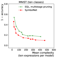
(a)

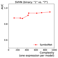
(b)

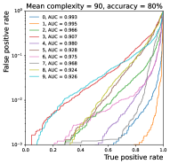
(c)

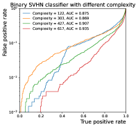
(d)

Figure 9: Performance of SymbolNet on the MNIST and the binary SVHN datasets. (a): A Pareto front is presented that illustrates the trade-off between accuracy and expression complexity when comparing SymbolNet to EQL in the MNIST dataset. (b): The ROC AUC is plotted against the expression complexity to demonstrate the performance of SymbolNet on the binary SVHN dataset. (c): ROC curves of a compact symbolic model with a mean complexity of 90 and an accuracy of 80%, the expressions of this model are tabulated in Table II. (d): ROC curves of four symbolic models with different complexity values. The expression of the model with a complexity of 122 is listed in Table III.

TABLE II: An example of a compact symbolic model with a mean complexity of 90 and an overall accuracy of 80%, learned by SymbolNet in the MNIST dataset. Constants are rounded to 2 significant figures for the purpose of display.

Class	Expression (symbolic model classifying MNIST digits)	Complexity	AUC
$0$	$0.094\sin(0.41x_{374}-0.53x_{378}+0.66x_{484})+0.15(-0.3x_{184}-0.17x_{239}-0.12x_{269}-0.27x_{271}-$	129	0.993
	$0.14x_{318}+0.72x_{352}-0.6x_{358}-0.19x_{374}+0.55x_{377}-0.32x_{415}-0.23x_{456}-0.26x_{485}-0.4x_{510}-$
	$0.53x_{627}+0.25x_{637}-0.19x_{658}+0.55x_{711})(0.44x_{102}-0.29x_{156}-0.41x_{212}-0.29x_{271}-0.22x_{302}-$
	$0.11x_{371}-0.5x_{398}-0.41x_{428}-0.24x_{430}+0.84x_{433}+0.6x_{436}+0.11x_{462}+0.62x_{490}-0.45x_{509}-$
	$0.066x_{539}-0.4x_{541}-0.13x_{568}+0.22x_{580}-0.58x_{627}-0.25x_{658})$
$1$	$\exp(-26.0(0.11x_{102}+0.056x_{158}+0.21x_{176}+0.08x_{178}+0.093x_{182}+0.93x_{205}+0.11x_{212}+0.15x_{235}+$	91	0.995
	$0.27x_{248}-0.033x_{267}+0.067x_{271}+0.24x_{302}-0.063x_{323}+0.095x_{327}-0.067x_{350}-0.12x_{378}+$
	$0.18x_{430}+x_{438}-0.067x_{462}-0.092x_{489}+0.18x_{510}-0.024x_{568}+0.12x_{580}+0.23x_{637}+0.24x_{711}+$
	$0.13x_{713}+0.24x_{715}+0.27x_{96}+0.28)^{2})$
$2$	$0.54\sin(0.59x_{124}+0.35x_{156}-0.39x_{318}-0.41x_{350}-0.46x_{371}-0.41x_{374}-0.6x_{415}+0.18x_{431}+$	58	0.966
	$0.14x_{465}+1.1x_{473}+0.7x_{509}+0.38x_{515}+0.88x_{528}+0.38x_{554}+0.77x_{611}+0.39x_{637}+0.1x_{99}-$
	$0.8)+0.53$
$3$	$-0.042x_{158}+0.062x_{178}-0.039x_{235}-0.12x_{291}-0.063x_{316}+0.045x_{318}+0.061x_{404}-0.066x_{458}+$	56	0.907
	$0.032x_{485}-0.1x_{487}-0.074x_{489}-0.12x_{490}+0.038x_{515}+0.036x_{517}-0.06x_{541}+0.36x_{563}-$
	$0.043x_{572}+0.048x_{611}+0.28$
$4$	$0.76\exp(-4.7(0.47x_{124}+0.42x_{126}+0.49x_{128}+0.14x_{176}+0.28x_{182}+0.44x_{184}+0.17x_{212}+x_{239}+$	141	0.980
	$0.88x_{267}+0.81x_{322}+0.43x_{323}+0.33x_{350}+0.4x_{543}+0.3x_{554}+0.5x_{568}+0.35x_{623})^{2})-0.082\times$
	$(-0.2x_{124}-0.34x_{182}+0.39x_{429}-0.69x_{568}-0.66x_{713}+0.68)(1.4x_{102}+0.58x_{182}+0.75x_{208}+$
	$0.51x_{215}+0.29x_{235}+0.47x_{322}-0.53x_{323}-0.7x_{325}+0.23x_{355}+0.53x_{358}-1.4x_{374}-1.5x_{398}-$
	$0.63x_{431}-1.5x_{456}-0.68x_{462}-1.1x_{465}+0.48x_{541}+0.83x_{568}+4.9x_{66}+1.3x_{71}+1.3x_{713}+1.4x_{96})$
$5$	$\exp(-2.4(-0.15x_{124}+0.13x_{158}+0.59x_{190}+0.98x_{248}-0.13x_{267}-0.35x_{323}-0.68x_{325}-x_{327}-$	79	0.928
	$0.78x_{355}+0.17x_{404}-0.5x_{456}-0.19x_{490}-0.41x_{510}-0.6x_{515}+0.15x_{568}-0.63)^{2})-0.012x_{128}-$
	$0.12x_{358}+0.03x_{371}+0.069x_{374}-0.031x_{436}-0.019x_{485}+0.042x_{580}+0.026x_{623}$
$6$	$0.21x_{102}+0.3x_{103}+0.42x_{107}-0.054x_{215}-0.057x_{217}-0.093x_{269}-0.065x_{271}-0.068x_{302}-$	89	0.975
	$0.08x_{322}+0.068x_{358}+0.04x_{374}+0.12x_{414}+0.021x_{431}+0.069x_{485}-0.063x_{489}-0.078x_{510}+$
	$0.081x_{515}+0.047x_{543}-0.056x_{568}+0.065x_{572}-0.05x_{580}+0.35x_{64}+0.43x_{66}+0.22x_{68}+0.34x_{69}+$
	$0.29x_{71}+0.35x_{73}+0.56x_{78}+0.18x_{99}+0.1$
$7$	$0.98\exp(-3.1(-x_{124}-0.61x_{126}-0.81x_{128}-0.97x_{156}-0.24x_{184}-0.23x_{350}+0.073x_{355}-0.28x_{376}-$	68	0.968
	$0.13x_{377}-0.62x_{378}-0.72x_{404}-0.6x_{415}-0.62x_{431}-0.092x_{433}-0.43x_{458}-0.87x_{485}-0.94x_{539}-$
	$0.27x_{541}-0.84x_{581}-0.37x_{623})^{2})$
$8$	$-0.68\sin(0.16x_{156}-0.35x_{176}+0.43x_{302}+0.19x_{318}+0.23x_{327}+0.41x_{376}-0.2x_{414}-0.4x_{428}+$	55	0.924
	$0.46x_{433}-0.33x_{467}+0.27x_{487}+0.3x_{515}-0.34x_{528}+0.25x_{541}+0.58x_{658}+0.43x_{689}+1.1)+0.64$
$9$	$-0.051\sin(0.59x_{124}+0.35x_{156}-0.39x_{318}-0.41x_{350}-0.46x_{371}-0.41x_{374}-0.6x_{415}+0.18x_{431}+$	136	0.926
	$0.14x_{465}+1.1x_{473}+0.7x_{509}+0.38x_{515}+0.88x_{528}+0.38x_{554}+0.77x_{611}+0.39x_{637}+0.1x_{99}-0.8)-$
	$0.054x_{126}-0.066x_{158}-0.082x_{190}-0.11x_{205}+0.059x_{208}+0.016x_{215}-0.039x_{217}-0.0092x_{235}-$
	$0.11x_{248}-0.047x_{271}+0.093x_{316}-0.04x_{322}+0.069x_{327}+0.07x_{352}-0.059x_{414}+0.069x_{429}+$
	$0.038x_{431}+0.048x_{436}-0.057x_{467}-0.044x_{517}-0.067x_{541}+0.065x_{637}-0.06x_{658}+0.11x_{711}+$
	$0.1x_{713}+0.16x_{715}+0.029$

TABLE III: An example of a compact symbolic model with a complexity of 122 and an ROC AUC of 0.875, learned by SymbolNet in the binary SVHN dataset (classes “1” and “7”). Constants are rounded to 2 significant figures for the purpose of display.

Expression (symbolic model classifying SVHN digits in a binary setting: “1” vs. “7”)	Complexity	AUC
$0.58\exp(-4.7(0.35x_{1191}+0.2x_{1282}+0.29x_{1285}+0.53x_{1384}+0.3x_{1566}+0.35x_{1788}-0.56x_{2156}+0.38x_{2179}+$	122	0.875
$0.51x_{2460}+0.22x_{2470}+0.33x_{2746}-0.6x_{429}-0.26x_{612}-0.45x_{628}-0.32x_{637}-0.33x_{732}-0.26x_{733}-0.28x_{813}-$
$0.15x_{913}-1)^{2})+0.61\cos(1.4x_{1282}-1.4x_{1298}-1.6x_{1486}+1.7x_{1863}-1.2x_{2357}-0.53x_{2460}+0.79x_{2609}+$
$0.79x_{3046}-0.94x_{485}+0.71x_{511}-1.4x_{527}+1.9x_{617}+0.76x_{637}-1.8x_{720}+1.8x_{824}+0.68x_{831}-0.99x_{913})$

We analyze the MNIST dataset by considering all ten classes, so each symbolic model has ten expressions, each of which corresponds to one of the ten classes. Fig. 9a shows a Pareto front generated by SymbolNet in the MNIST dataset, which outperforms EQL in the multistage pruning framework. For example, SymbolNet can achieve an overall accuracy of 90% with a mean complexity of around 300. Table II tabulates the ten expressions of one of the symbolic models learned by SymbolNet, which has a mean complexity of 90 and an overall accuracy of 80%, and their ROC curves are shown in Figure 9c. This example demonstrates the power of symbolic models learned by SymbolNet, which is small enough to be visualized entirely in a table but capable of making a reasonable prediction.

For the SVHN dataset in the binary setting, each symbolic model has one expression. We found that EQL did not converge for this dataset, as it generated overly complex expressions with reasonable accuracy or expressions from models that were too sparse to make meaningful predictions. However, SymbolNet was able to scale to such a high-dimensional dataset and generate reasonable predictions with compact expressions. Fig. 9b shows the ROC AUC as a function of the expression complexity for the models learned by SymbolNet, and Fig. 9d shows the ROC curves of four symbolic models with different complexity values. Table III lists the expression of one of the symbolic models, which has a complexity of 122 and a ROC AUC of 0.875. It is also remarkable that such a single-line expression can already give decent predictions in classifying the SVHN digits from the noisy real-world scenes, as depicted in Fig. 6c.

V-C FPGA resource utilization and latency

TABLE IV: Resource utilization and latency on an FPGA for quantized and pruned (QP) NNs and symbolic expressions learned by SymbolNet. The model size is quoted in terms of the number of neurons per hidden layer for DNN, and the number of filters for CNN, where, for example, $(16)_{3}$ means 16 filters with a kernel size of 3$\times$3. The initiation interval (II) is quoted in clock cycles. The numbers in parentheses indicate the percentage of total available resource utilization. The relative accuracy and the ROC AUC are evaluated with respect to the same DNN/CNN implemented in floating point precision and without pruning.

LHC jet tagging (five classes)
	Model size (input dim. $=$ 16)	Precision	BRAMs	DSPs	FFs	LUTs	II	Latency	Rel. acc.
QP DNN	[64, 32, 32, 5], 90% pruned	$\langle$6, 0$\rangle$	4 (0.1%)	28 (0.4%)	2739 (0.1%)	7691 (0.7%)	1	55 ns	94.7%
SR	Mean complexity of the five expr. $=$ 18	$\langle$12, 8$\rangle$	0 (0%)	3 (0%)	109 (0%)	177 (0%)	1	10 ns	93.3%
MNIST (ten classes)
	Model size (input dim. $=$ 28$\times$28$\times$1)	Precision	BRAMs	DSPs	FFs	LUTs	II	Latency	Rel. acc.
QP CNN	[(16, 16, 24$)_{\text{3}}$, 42, 64, 10], 92% pruned	$\langle$6, 0$\rangle$	66 (1.5%)	216 (3.2%)	18379 (0.8%)	29417 (2.5%)	788	4.0 $\mu$s	86.8%
SR	Mean complexity of the ten expr. $=$ 133	$\langle$18, 10$\rangle$	0 (0%)	160 (2.3%)	6424 (0.3%)	7592 (0.6%)	1	125 ns	85.3%
SVHN (binary “1” vs. “7”)
	Model size (input dim. $=$ 32$\times$32$\times$3)	Precision	BRAMs	DSPs	FFs	LUTs	II	Latency	Rel. AUC
QP CNN	[(16, 16, 24$)_{\text{3}}$, 42, 64, 1], 92% pruned	$\langle$6, 0$\rangle$	62 (1.4%)	77 (1.1%)	16286 (0.7%)	27407 (2.3%)	1029	5.2 $\mu$s	94.0%
SR	Complexity $=$ 311	$\langle$10, 4$\rangle$	0 (0%)	38 (0.6%)	1945 (0.1%)	3029 (0.3%)	1	195 ns	94.5%

Table IV tabulates resource utilization and latency on an FPGA, comparing between conventionally compressed NNs and symbolic models. FPGA resources include on-board FPGA memory (BRAMs), digital signal processors (DSPs), flip-flops (FFs), and lookup tables (LUTs), estimated from the logic synthesis step. Symbolic models generally consume significantly less resources and require much less latency than NNs, even when the NNs are already strongly quantized and pruned, while achieving comparable accuracy across the three datasets.

VI Conclusion

We have proposed SymbolNet, a neural network approach to symbolic regression with a novel and dedicated pruning framework to generate compact expressions to fit high-dimensional data. Most existing methods, based on genetic programming or deep learning, focus primarily on datasets with input dimensions less than $O(10)$ and cannot scale efficiently beyond. This is because in genetic programming approaches, the search algorithms create and evolve equations in a combinatorial strategy, which becomes extremely inefficient as the equation search space scales exponentially with its building blocks. On the other hand, deep learning techniques have not been extensively explored in the field of symbolic regression to solve high-dimensional problems, despite their demonstrated capability to handle complex datasets in other domains. Our proposed method with a novel pruning framework dedicated to symbolic regression attempts to fill this gap, its effectiveness has been demonstrated on datasets with input dimensions ranging from $O(10)$ to $O(1000)$. There is always a trade-off between prediction accuracy and computational resources, this work attempts to provide an option to minimize the latter. It opens up a potential application of symbolic regression for model compression, allowing for deploying more compact symbolic models in resource-constrained environments. It will also be interesting to investigate high-dimensional differential equations.

Currently, neural networks have certain limitations when used to solve symbolic regression in comparison to genetic programming. For instance, it is not trivial to create a unified framework that can incorporate any non-differentiable mathematical operator, such as division and conditionals, without specifically regularizing each of these operators, as this would lead to singular points in the gradient optimization, thus limiting the approach to fit data. Additionally, genetic programming can generate a batch of models due to its discrete nature, but the process is rather slow, while one neural network can only generate one model at a time, even though the training is usually fast due to its continuous nature by using gradient descent. These issues shall be addressed in future work.

References

- [1] M. Planck, “On an improvement of Wien’s equation for the spectrum,” Verh. Dtsch. Phys. Ges., vol. 2, 1900.
- [2] M. Virgolin and S. P. Pissis, “Symbolic regression is NP-hard,” arXiv:2207.01018, 2022.
- [3] M. Abadi, A. Agarwal, P. Barham, E. Brevdo, Z. Chen, C. Citro, G. S. Corrado, A. Davis, J. Dean, M. Devin, S. Ghemawat, I. Goodfellow, A. Harp, G. Irving, M. Isard, Y. Jia, R. Jozefowicz, L. Kaiser, M. Kudlur, J. Levenberg, D. Mané, R. Monga, S. Moore, D. Murray, C. Olah, M. Schuster, J. Shlens, B. Steiner, I. Sutskever, K. Talwar, P. Tucker, V. Vanhoucke, V. Vasudevan, F. Viégas, O. Vinyals, P. Warden, M. Wattenberg, M. Wicke, Y. Yu, and X. Zheng, “TensorFlow: Large-scale machine learning on heterogeneous systems,” 2015, software available from tensorflow.org. [Online]. Available: https://www.tensorflow.org/
- [4] J. Liu, Z. Xu, R. Shi, R. C. C. Cheung, and H. K. H. So, “Dynamic sparse training: Find efficient sparse network from scratch with trainable masked layers,” arXiv:2005.06870, 2020.
- [5] J. Koza, “Genetic programming as a means for programming computers by natural selection,” Statistics and Computing, vol. 4, pp. 87–112, 1994.
- [6] M. Schmidt and H. Lipson, “Distilling free-form natural laws from experimental data,” Science, vol. 324, pp. 81–85, 2009. [Online]. Available: https://doi.org/10.1126/science.1165893
- [7] M. Cranmer, “Interpretable machine learning for science with PySR and SymbolicRegression.jl,” arXiv:2305.01582, 2023.
- [8] D. Wadekar, F. Villaescusa-Navarro, S. Ho, and L. Perreault-Levasseur, “Modeling assembly bias with machine learning and symbolic regression,” arXiv:2012.00111, 2020.
- [9] H. Shao, F. Villaescusa-Navarro, S. Genel, D. N. Spergel, D. Anglé s-Alcázar, L. Hernquist, R. Davé, D. Narayanan, G. Contardo, and M. Vogelsberger, “Finding universal relations in subhalo properties with artificial intelligence,” The Astrophysical Journal, vol. 927, no. 1, p. 85, 2022. [Online]. Available: https://doi.org/10.3847%2F1538-4357%2Fac4d30
- [10] A. M. Delgado, D. Wadekar, B. Hadzhiyska, S. Bose, L. Hernquist, and S. Ho, “Modelling the galaxy–halo connection with machine learning,” Monthly Notices of the Royal Astronomical Society, vol. 515, no. 2, pp. 2733–2746, 2022. [Online]. Available: https://doi.org/10.1093%2Fmnras%2Fstac1951
- [11] D. Wadekar, L. Thiele, J. C. Hill, S. Pandey, F. Villaescusa-Navarro, D. N. Spergel, M. Cranmer, D. Nagai, D. Anglé s-Alcázar, S. Ho, and L. Hernquist, “The SZ flux-mass () relation at low-halo masses: improvements with symbolic regression and strong constraints on baryonic feedback,” Monthly Notices of the Royal Astronomical Society, vol. 522, no. 2, pp. 2628–2643, 2023. [Online]. Available: https://doi.org/10.1093%2Fmnras%2Fstad1128
- [12] P. Lemos, N. Jeffrey, M. Cranmer, S. Ho, and P. Battaglia, “Rediscovering orbital mechanics with machine learning,” arXiv:2202.02306, 2022.
- [13] D. Wadekar, L. Thiele, F. Villaescusa-Navarro, J. C. Hill, M. Cranmer, D. N. Spergel, N. Battaglia, D. Anglé s-Alcázar, L. Hernquist, and S. Ho, “Augmenting astrophysical scaling relations with machine learning: Application to reducing the sunyaev–zeldovich flux–mass scatter,” Proceedings of the National Academy of Sciences, vol. 120, no. 12, 2023. [Online]. Available: https://doi.org/10.1073%2Fpnas.2202074120
- [14] A. Grundner, T. Beucler, P. Gentine, and V. Eyring, “Data-driven equation discovery of a cloud cover parameterization,” arXiv:2304.08063, 2023.
- [15] T. Stephens, “Genetic programming in Python, with a scikit-learn inspired API: gplearn,” 2016. [Online]. Available: https://gplearn.readthedocs.io/en/stable/
- [16] B. Burlacu, G. Kronberger, and M. Kommenda, “Operon C++: An efficient genetic programming framework for symbolic regression,” in Proceedings of the 2020 Genetic and Evolutionary Computation Conference Companion, ser. GECCO ’20. New York, NY, USA: Association for Computing Machinery, 2020, p. 1562–1570. [Online]. Available: https://doi.org/10.1145/3377929.3398099
- [17] M. Virgolin, T. Alderliesten, C. Witteveen, and P. A. N. Bosman, “Improving model-based genetic programming for symbolic regression of small expressions,” Evolutionary Computation, vol. 29, no. 2, pp. 211–237, 2021. [Online]. Available: https://doi.org/10.1162%2Fevco_a_00278
- [18] G. Martius and C. H. Lampert, “Extrapolation and learning equations,” 2016.
- [19] S. S. Sahoo, C. H. Lampert, and G. Martius, “Learning equations for extrapolation and control,” 2018.
- [20] M. Werner, A. Junginger, P. Hennig, and G. Martius, “Informed equation learning,” 2021.
- [21] S. Kim, P. Y. Lu, S. Mukherjee, M. Gilbert, L. Jing, V. Ceperic, and M. Soljacic, “Integration of neural network-based symbolic regression in deep learning for scientific discovery,” IEEE Transactions on Neural Networks and Learning Systems, vol. 32, no. 9, pp. 4166–4177, 2021. [Online]. Available: https://doi.org/10.1109%2Ftnnls.2020.3017010
- [22] I. A. Abdellaoui and S. Mehrkanoon, “Symbolic regression for scientific discovery: an application to wind speed forecasting,” arXiv:2102.10570, 2021.
- [23] A. Costa, R. Dangovski, O. Dugan, S. Kim, P. Goyal, M. Soljačić, and J. Jacobson, “Fast neural models for symbolic regression at scale,” arXiv:2007.10784, 2021.
- [24] B. K. Petersen, M. L. Larma, T. N. Mundhenk, C. P. Santiago, S. K. Kim, and J. T. Kim, “Deep symbolic regression: Recovering mathematical expressions from data via risk-seeking policy gradients,” in International Conference on Learning Representations, 2021. [Online]. Available: https://openreview.net/forum?id=m5Qsh0kBQG
- [25] H. Zhou and W. Pan, “Bayesian learning to discover mathematical operations in governing equations of dynamic systems,” arXiv:2206.00669, 2022.
- [26] J. Kubalík, E. Derner, and R. Babuška, “Toward physically plausible data-driven models: A novel neural network approach to symbolic regression,” IEEE Access, vol. 11, pp. 61 481–61 501, 2023. [Online]. Available: https://doi.org/10.1109%2Faccess.2023.3287397
- [27] L. Biggio, T. Bendinelli, A. Neitz, A. Lucchi, and G. Parascandolo, “Neural symbolic regression that scales,” in Proceedings of the 38th International Conference on Machine Learning, ser. Proceedings of Machine Learning Research, M. Meila and T. Zhang, Eds., vol. 139. PMLR, 18–24 Jul 2021, pp. 936–945. [Online]. Available: https://proceedings.mlr.press/v139/biggio21a.html
- [28] M. Valipour, B. You, M. Panju, and A. Ghodsi, “Symbolicgpt: A generative transformer model for symbolic regression,” 2021.
- [29] P.-A. Kamienny, S. d’Ascoli, G. Lample, and F. Charton, “End-to-end symbolic regression with transformers,” in Advances in Neural Information Processing Systems, 2022.
- [30] M. Vastl, J. Kulhánek, J. Kubalík, E. Derner, and R. Babuška, “Symformer: End-to-end symbolic regression using transformer-based architecture,” arXiv:2205.15764, 2022.
- [31] A. Meurer, C. P. Smith, M. Paprocki, O. Čertík, S. B. Kirpichev, M. Rocklin, A. Kumar, S. Ivanov, J. K. Moore, S. Singh, T. Rathnayake, S. Vig, B. E. Granger, R. P. Muller, F. Bonazzi, H. Gupta, S. Vats, F. Johansson, F. Pedregosa, M. J. Curry, A. R. Terrel, v. Roučka, A. Saboo, I. Fernando, S. Kulal, R. Cimrman, and A. Scopatz, “Sympy: symbolic computing in python,” PeerJ Computer Science, vol. 3, p. e103, Jan. 2017. [Online]. Available: https://doi.org/10.7717/peerj-cs.103
- [32] H. F. Tsoi, A. A. Pol, V. Loncar, E. Govorkova, M. Cranmer, S. Dasu, P. Elmer, P. Harris, I. Ojalvo, and M. Pierini, “Symbolic regression on FPGAs for fast machine learning inference,” arXiv:2305.04099, 2023.
- [33] M. Pierini, J. M. Duarte, N. Tran, and M. Freytsis, “HLS4ML LHC Jet dataset (150 particles),” 2020. [Online]. Available: https://doi.org/10.5281/zenodo.3602260
- [34] Y. LeCun and C. Cortes, “MNIST handwritten digit database,” 2010. [Online]. Available: http://yann.lecun.com/exdb/mnist/
- [35] Y. Netzer, T. Wang, A. Coates, A. Bissacco, B. Wu, and A. Y. Ng, “Reading digits in natural images with unsupervised feature learning,” in NIPS Workshop on Deep Learning and Unsupervised Feature Learning 2011, 2011. [Online]. Available: http://ufldl.stanford.edu/housenumbers/nips2011_housenumbers.pdf
- [36] ATLAS Collaboration, “Technical Design Report for the Phase-II Upgrade of the ATLAS TDAQ System,” CERN-LHCC-2017-020, ATLAS-TDR-029, 2017.
- [37] CMS Collaboration, “The Phase-2 Upgrade of the CMS Level-1 Trigger,” CERN-LHCC-2020-004, CMS-TDR-021, 2020.
- [38] J. Duarte et al., “Fast inference of deep neural networks in FPGAs for particle physics,” JINST, vol. 13, no. 07, p. P07027, 2018.
- [39] E. A. Moreno, O. Cerri, J. M. Duarte, H. B. Newman, T. Q. Nguyen, A. Periwal, M. Pierini, A. Serikova, M. Spiropulu, and J.-R. Vlimant, “JEDI-net: a jet identification algorithm based on interaction networks,” Eur. Phys. J. C, vol. 80, no. 1, p. 58, 2020.
- [40] E. Coleman, M. Freytsis, A. Hinzmann, M. Narain, J. Thaler, N. Tran, and C. Vernieri, “The importance of calorimetry for highly-boosted jet substructure,” JINST, vol. 13, no. 01, p. T01003, 2018.
- [41] T. Aarrestad et al., “Fast convolutional neural networks on FPGAs with hls4ml,” Mach. Learn. Sci. Tech., vol. 2, no. 4, p. 045015, 2021.
- [42] C. N. Coelho, A. Kuusela, S. Li, H. Zhuang, T. Aarrestad, V. Loncar, J. Ngadiuba, M. Pierini, A. A. Pol, and S. Summers, “Automatic heterogeneous quantization of deep neural networks for low-latency inference on the edge for particle detectors,” Nature Mach. Intell., vol. 3, pp. 675–686, 2021.
- [43] M. Zhu and S. Gupta, “To prune, or not to prune: exploring the efficacy of pruning for model compression,” 2017.
- [44] FastML Team, “fastmachinelearning/hls4ml,” 2021. [Online]. Available: https://github.com/fastmachinelearning/hls4ml
- [45] Xilinx, “Vivado Design Suite User Guide: High-Level Synthesis,” https://www.xilinx.com/support/documentation/sw_manuals/xilinx2020_1/ug902-vivado-high-level-synthesis.pdf, 2020.
- [46] D. P. Kingma and J. Ba, “Adam: A method for stochastic optimization,” 2017.