Abstract

We investigate the data-driven holographic transport models without translation symmetry. Our data are chosen as the real part of the frequency-dependent shear viscosity. We develop a radial flow equation for a large class of holographic models, which determine the shear viscosity by the black hole metric and the graviton mass. The latter serves as the bulk dual of the translation symmetry breaking on the boundary. We convert the flow equation to a Neural Ordinary Differential Equation (Neural ODE), which is a neural network with continuous depth and produces output through a black-box ODE solver. Given either the metric or the mass, we illustrate that the Neural ODE can learn the other with high accuracy. Our work demonstrates the capabilities of Neural ODEs in bulk reconstruction and applied holography.

1 Introduction

AdS/CFT correspondence is an elegant holographic mapping that brings illuminating insights into quantum gravity and provides fruitful phenomenal models of strongly coupled quantum field theories [1, 2]. The typical process for the holographic modeling involves assuming a bulk action, solving the Einstein equation to obtain the bulk spacetime metric, and using the holographic dictionary to convert various gravity observables into field-theory observables. However, building a suitable action from a phenomenological perspective is a fundamental and challenging inverse problem in theoretical physics. In addition to relying on the symmetry principle, it usually requires deep domain knowledge and intuition from human experts.

In holography, under certain conditions, some field-theory observables can be determined solely by the bulk metric, without requiring the full action. This leads to a reduced inverse problem: Can we reconstruct the bulk metric from these field-theory observables? This line of work belongs to an important branch of the well-known bulk reconstruction project [4, 3, 5]. Its ambitious goal is to reorganize the CFT degrees of freedom into local gravitational physics under certain limits. There are many different methods for reconstructing the bulk metric, part of which can be found in [6, 7, 8, 9, 12, 10, 11, 13, 14, 15, 16, 17, 18, 19, 20, 22, 21, 23, 24, 25, 26]. Among others, Hashimoto et al. propose an interesting scheme using the neural network and deep learning (DL) [27]. They discretize the Klein-Gordon equation of a scalar field in a curved spacetime as the architecture of a neural network. Their data consist of the VEV of the operator and its conjugate source, with the IR behavior of the field as the labels. They use a smoothness term on the metric as a regularization to guide the training. After training, the black hole metric is encoded as the weights of the neural network. This scheme is called as the AdS/DL correspondence. It has been quickly applied to construct holographic QCD models and obtained interesting results, which include extracting the novel feature from the lattice data of chiral condensate, predicting the reasonable mass for excited state mesons, and deriving the explicit form of a dilaton potential, etc [28, 29, 30, 31, 32, 33].

In addition to QCD, holographic models have been widely used in condensed matter physics, hydrodynamics, and quantum information. Among others, transport phenomena, such as momentum and charge transports, are considered very suitable for the holographic research based on the bottom-up setup. In view of this, Yan et al. propose a data-driven holographic transport model by deep learning [34]. Their data are the complex frequency-dependent shear viscosity and the network architecture corresponds to the discretization of a radial flow equation. Since the IR solution of the flow equation can be fully determined by regularity, the forward propagation of information is designed from IR to UV. Compared with previous algorithms, this algorithm eliminates the need to introduce additional IR labels for the data, thereby reducing systematic errors in the analysis. Recently, a similar algorithm has been developed to learn from the optical conductivity [35], aiming to apply AdS/DL to the condensed matters, such as strange metal and high-temperature superconductivity.

All of the above work about AdS/DL has one commonality: the emergent extra dimension corresponds to the depth of the neural network. In fact, the neural network itself is regarded as a bulk spacetime. However, since the neural network has discrete layers, both the spacetime metric and the equation of motion are discrete. This leads to intrinsic discrete errors in the algorithm. Moreover, the regularization term that induces smooth metrics increases arbitrariness and computational cost.

To address these discrete problems, Neural ODEs have been introduced for AdS/DL [36]. This is a relatively new family of deep neural network models that generalize the standard layer-to-layer propagation to continuous-depth models [37]. In essence, Neural ODEs employ a neural network to parameterize the derivative of the hidden state, while the output is computed using a black-box adaptive differential equation solver. The application of Neural ODEs in holographic modeling, as highlighted in [36], showcases the potential of AI as more than just a data processing tool in theoretical physics, but also as a valuable aid in scientific discoveries.

The purpose of this paper is twofold. On a technical level, we aim to replace the discrete architecture in [34] with Neural ODEs. On a physical level, we intend to break the translation symmetry that is respected by the theoretical framework in [34]. The latter is indispensable to describe the real-world condensed matter. However, for AdS/DL to be significant, its theoretical framework for the holographic calculation must possess a certain universality. In [34], the universality depends heavily on the relationship between the shear viscosity of the boundary field theory and the shear response on the UV boundary. If the translation symmetry is broken, this relationship usually no longer holds. Fortunately, through the analysis of the UV behavior related to the holographic renormalization [38, 39], we find that the shear viscosity and the shear response on the boundary usually have the same real part, even if the translation symmetry is broken. This observation motivates us to use only the real part of the shear viscosity as the data for learning.

After the data is ready, we need to clarify the training tasks. In this paper, we will focus on the holographic models with homogeneous and isotropic geometry, which are relatively simple. Nevertheless, determining the shear viscosity requires the function of graviton mass in addition to the function of metric. As a reverse engineering, we will study if given a mass or a metric, can Neural ODEs learn the other one?

The rest of the paper will be arranged as follows. In Section 2, we will develop a radial flow equation in a large class of holographic models without translation symmetry. In Section 3, we will introduce the machine learning algorithm, including the network architecture, loss function and inductive bias. In Section 4, we will generate the data and depict the training results based on three typical holographic models without translation symmetry. The conclusion and discussion will be presented in Section 5. There are also two appendices. In Appendix A, we will build the relationship between the shear viscosity and the shear response. In Appendix B, we will provide the training scheme and report.

2 Holographic flow equation

Consider a strongly coupled field theory that is holographically dual to the 3+1 dimensional Einstein gravity minimally coupled with the matter. Suppose that it allows a planar black hole solution, which is described by the line element

$$ds^{2}=-g_{tt}(r)dt^{2}+g_{rr}(r)dr^{2}+g_{xx}(r)d\vec{x}^{2},$$ (1)

and sourced by the energy-momentum tensor

$$T_{\mu\nu}=\mathrm{diag}\left(T_{tt}(r),T_{rr}(r),T_{xx}(r),T_{xx}(r)\right).$$ (2)

Importantly, Eq. (1) and Eq. (2) are homogeneous and isotropic along the field theory directions, although we have not assumed that the matter fields are homogeneous. When the black hole is perturbed by the time-dependent shear mode $\left(\delta g\right)_{\;x_{2}}^{x_{1}}=h(r)e^{-i\omega t}$, the wave equation has a general form [40]

$$\frac{1}{\sqrt{-g}}\partial_{r}(\sqrt{-g}g^{rr}\partial_{r}h)+\left(\omega^{2}g^{tt}-m^{2}\right)h=0,$$ (3)

where $m$ is the radially varying graviton mass, given by

$$m\left(r\right)^{2}=g^{xx}T_{xx}-\frac{\delta T_{xy}}{\delta g_{xy}}.$$ (4)

Note that the nonzero graviton mass in the bulk is dual to the breaking of the translation symmetry on the boundary [41].

Consider the bulk spacetime sliced along the radial direction and introduce the shear response function at each slice

$$\chi=\frac{\Pi}{i\omega h},$$ (5)

where $\Pi=-\sqrt{-g}g^{rr}\partial_{r}h$ is the momentum conjugate to the field $h$ in the Hamiltonian formulation. Using Eq. (5), one can rewrite the wave equation as

$$\partial_{r}\chi-i\omega\sqrt{\frac{g_{rr}}{g_{tt}}}\left(\frac{\chi^{2}}{g_{xx}}-g_{xx}\right)+\frac{1}{i\omega}\sqrt{g_{tt}g_{rr}}g_{xx}m^{2}=0,$$ (6)

which is a radial flow equation of the shear response.

Observing the flow equation (6), one can see that the regularity of the shear response indicates

$$\chi(r_{\mathrm{h}})=g_{xx}(r_{\mathrm{h}}),$$ (7)

where $r_{\mathrm{h}}$ is the horizon radius. Using Eq. (7) as the IR boundary condition, the flow equation can be solved to obtain the complex shear response at UV. In general, however, it is not the desired shear viscosity. Nevertheless, by the UV analysis given in Appendix A, we will demonstrate that for a large class of theories, their real parts are the same indeed

$$\eta_{\mathrm{re}}=\left.\chi_{\mathrm{re}}\right|_{r\rightarrow\infty}.$$ (8)

Now, let’s simplify the metric (1) by imposing $g_{tt}g_{rr}=1$ and setting $g_{xx}=r^{2}$. Then one can obtain

$$ds^{2}=\frac{1}{z^{2}}\left[-f(z)dt^{2}+\frac{1}{f(z)}dz^{2}+d\vec{x}^{2}\right],$$ (9)

where the coordinate $z=r_{\mathrm{h}}/r$ has been used. Thus, the horizon is located at $z_{\mathrm{h}}=1$ and the boundary at $z_{\mathrm{b}}=0$. In terms of Eq. (9), the flow equation (6) can be reduced to

$$\partial_{z}\chi+\frac{i\omega}{f}\left(z^{2}\chi^{2}-\frac{1}{z^{2}}\right)-\frac{1}{i\omega}\frac{m^{2}}{z^{4}}=0,$$ (10)

where the horizon radius has been set as $r_{\mathrm{h}}=1$. Accordingly, the IR boundary condition (7) and the UV relation (8) are changed into $\chi(z_{\mathrm{h}})=1$ and $\eta_{\mathrm{re}}=\chi_{\mathrm{re}}\left(z_{\mathrm{b}}\right)$, respectively.

3 Machine learning algorithm

3.1 Neural ODE

In residual networks [42], there is a sequence of transformations to a hidden state

$$x_{t+1}=x_{t}+y_{t}(x_{t},\theta_{t}),$$ (11)

where $x_{t}$ is the hidden state at layer $t$, $y_{t}$ is a differentiable function preserves the dimension of $x_{t}$, and $\theta_{t}$ denotes the transform parameters. The difference between $x_{t+1}$ and $x_{t}$ can be interpreted as a discretization of the derivative $x^{\prime}(t)$ with the step $\Delta t=1$. Adding more layers and decreasing the step, one can approach the limit

$$\frac{dx(t)}{dt}=y(x(t),t,\theta).$$ (12)

This equation can be used to represent the Neural ODE, an ODE induced by the continuous-depth limit of residual networks.

Given an initial state $x(t_{0})$, the forward propagation of Neural ODEs yields the state $x(t_{1})$ through a black-box ODE solver. The back propagation of Neural ODEs is realized by the adjoint sensitivity method [43]. Suppose that there is a loss function depending on the outputs of an ODE solver

$$L\left(x\left(t_{1}\right)\right)=L(x\left(t_{0}\right)+\int_{t_{0}}^{t_{1}}y(x(t),t,\theta)dt).$$ (13)

The adjoint state is defined as

$$a(t)=\frac{\partial L}{\partial x\left(t\right)}.$$ (14)

It has been proven that the adjoint dynamics is dominated by another ODE

$$\frac{da(t)}{dt}=-a(t)\cdot\frac{\partial y}{\partial x},$$ (15)

and the parameter gradient can be calculated by an integral [37]

$$\frac{\partial L}{\partial\theta}=\int_{t_{1}}^{t_{0}}a(t)\cdot\frac{\partial y}{\partial\theta}dt.$$ (16)

Now we can transform the flow equation into the Neural ODE. We first split the flow equation (10) into real and imaginary parts

$$\frac{d\chi_{\mathrm{re}}}{dz} = \frac{2\omega z^{2}}{f}\chi_{\mathrm{re}}\chi_{\mathrm{im}},$$ (17)

$$\frac{d\chi_{\mathrm{im}}}{dz} = \frac{\omega}{f}\left[\left(z\chi_{\mathrm{im}}\right)^{2}-\left(z\chi_{\mathrm{re}}\right)^{2}+\frac{1}{z^{2}}\right]-\frac{m^{2}}{\omega z^{4}}.$$ (18)

Then we identify the shear response $\left(\chi_{\mathrm{re}},\chi_{\mathrm{im}}\right)$ with the state $x$ and the radial coordinate $z$ with the time $t$. In general, the function of metric $f(z)$ or the function of mass square $m^{2}(z)$ can be represented by a neural network with the parameter $\theta$.

Obviously, given the parameter $\theta$ is equivalent to giving the trial function of metric or mass square which specifies the Neural ODE. By invoking an ODE solver, one can integrate from IR to UV and predict the real part of shear viscosity. Using the adjoint sensitivity method, one can implement back-propagation and perform training. We depict the architecture of the current algorithm in Fig. 1. Note that it differs from the usual Neural ODE in that one component of the adjoint state vanishes.

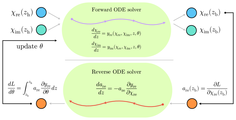
Figure 1: The architecture of the algorithm. The upper part depicts the forward propagation (from IR to UV) of the real and imaginary parts of the shear response. The lower part depicts the backward propagation of the adjoint state related only to the real part.

3.2 Loss function and inductive bias

Our loss function is chosen as the log-cosh form [44, 45, 46, 47]

$$L=\frac{1}{N}\sum_{i=1}^{N}\log\left[\cosh\left(\eta_{\mathrm{re}}\left(\omega_{i},\theta\right)-\bar{\eta}_{\mathrm{re}}\left(\omega_{i}\right)\right)\right],$$ (19)

where $N$ denotes the size of data, $\bar{\eta}_{\mathrm{re}}$ represents the input data, and $\eta_{\mathrm{re}}$ is what the Neural ODE predicts. Note that the loss $\log\left[\cosh\left(x\right)\right]$ behaves like L1 loss $\left|x\right|$ far from the origin and L2 loss $x^{2}$ close to the origin. It is twice differentiable everywhere, making it suitable for optimizers like BFGS that require the Hessian [48].

We need to impose some inductive biases, which depend on different tasks.

Task 1: Learning the metric

Suppose that the graviton mass is given. Since we focus on finite temperature field theories, there should be a horizon at $z=1$. This bias is implemented through the ansatz

$$f(z)=(1-z)n_{1}(z,\theta_{1}),$$ (20)

where $n_{1}$ is a neural network with the trainable parameter $\theta_{1}$.

Task 2: Learning the mass

Suppose that the metric is given. We propose the ansatz

$$m(z)^{2}=z^{b}n_{2}(z,\theta_{2})$$ (21)

where the exponent $b$ is a hyperparameter and $n_{2}$ is a neural network with the trainable parameter $\theta_{2}$. The purpose of separating $z^{b}$ from $m(z)^{2}$ is to input the UV information $m(z)^{2}\sim z^{b}+\cdots$ through hyperparameter tuning, see Appendix B.

4 Holographic models

We will study three holographic models without translation symmetry, all of which have homogeneous and isotropic geometry.

4.1 Massive gravity

The research of massive gravity (MG) has a long and winding history [49, 50, 51, 52, 53]. The main theoretical interest is to explore whether there exists a self-consistent theory that has a massive graviton with spin 2. In cosmology, MG is considered as a candidate theory that explains the accelerated expansion of the universe by modifying Einstein gravity. In holography, massive gravity is the first analytically tractable model without translation symmetry [54]

We will consider the dRGT massive gravity that is claimed to be ghost free [55, 56, 57]. Its simplest version used in holography is described by the bulk action

$$S_{\mathrm{bulk}}=\int d^{4}x\sqrt{-g}\left(\mathcal{R}+6-\alpha\mathrm{tr}\mathcal{X}\right),$$ (22)

where $\mathcal{X}{{}^{\mu}}_{\nu}=\sqrt{g^{\mu\lambda}f_{\lambda\nu}}$ and $f_{\mu\nu}=\mathrm{diag}(0,0,1,1)$ is the reference metric. Note that we have set the gravitational constant $16\pi G=1$ and the AdS radius $L=1$. The Gibbons-Hawking term is given by

$$S_{\mathrm{GH}}=2\int d^{3}x\sqrt{-\gamma}K,$$ (23)

where $\gamma_{ij}$ is the induced metric and $K$ is the external curvature. The counterterms have been derived in [58]

$$S_{\mathrm{ct}}=\int d^{3}x\sqrt{-\gamma}\left[-4-R+\frac{1}{2}\alpha e_{1}+\frac{1}{16}\alpha^{2}e_{2}+\frac{\alpha}{4}(2R_{ij}Y^{ij}-e_{1}R)\log r\right],$$ (24)

where $e_{1}=\mathrm{tr}Y$, $e_{2}=\left(\mathrm{tr}Y\right)^{2}-\mathrm{tr}Y^{2}$, and $Y{{}^{i}}_{j}=\sqrt{\gamma^{ik}f_{kj}}$.

Using the action, one can derive the Einstein equation

$$R_{\mu\nu}-\frac{1}{2}g_{\mu\nu}R-3g_{\mu\nu}=\frac{1}{2}\alpha\left(\mathcal{X}_{\mu\nu}-g_{\mu\nu}\mathrm{tr}\mathcal{X}\right).$$ (25)

This allows for the existence of a black hole solution (9) with the emblackening factor

$$f(z)=1-z^{3}-\frac{\alpha}{2}z(1-z^{2}).$$ (26)

The black hole is associated with the Hawking temperature

$$T=\frac{1}{4\pi}\left(3-\alpha\right),$$ (27)

which should be non-negative. Inserting the energy-momentum tensor

$$T_{\mu\nu}=\alpha\left(\mathcal{X}_{\mu\nu}-g_{\mu\nu}\mathrm{tr}\mathcal{X}\right)$$ (28)

into Eq. (4), one can calculate the square of graviton mass

$$m^{2}=\frac{\alpha}{2}z.$$ (29)

Now we can generate the data for learning. Inputting Eq. (26) and Eq. (29) into Eq. (10), using the regular condition at the horizon, and setting the typical parameter $\alpha=1$, one can solve the flow equation and obtain the real part of shear viscosity on the boundary. We sample the frequency uniformly between 0.01 and 6 to generate 600 data points $\left[\omega,\eta_{\mathrm{re}}(\omega)\right]$, which are plotted in Fig. 2.

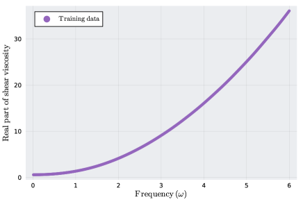
Figure 2: The real part of frequency-dependent shear viscosity. It is generated by solving the flow equation with the true metric and mass in the MG model.

We conduct two numerical experiments: fixing the mass to learn the metric and fixing the metric to learn the mass. The primary training results are shown in Fig. 3 below. Additionally, Fig. 8 and Tab. 1 in Appendix B detail the hyperparameter tuning, minimum loss, and mean relative error (MRE).

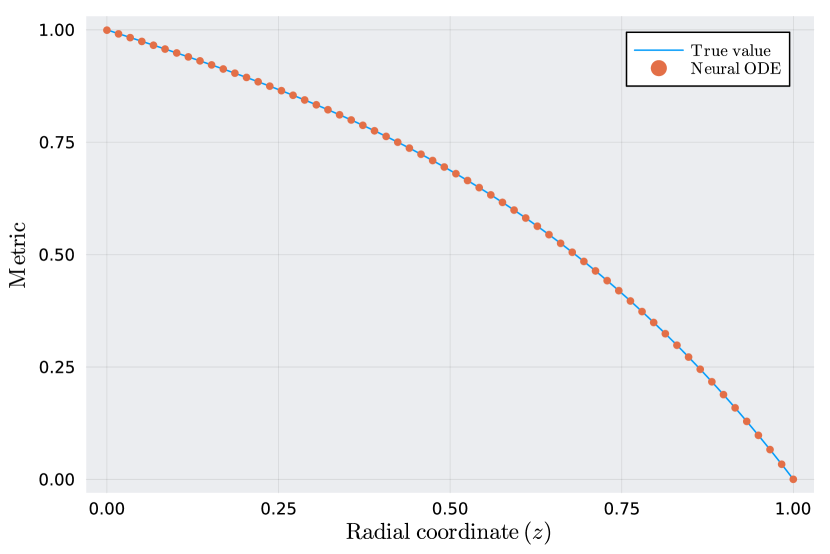
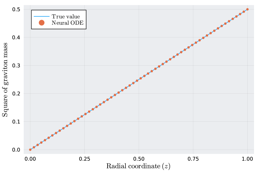
Figure 3: The performance of Neural ODEs for learning metric (left) and mass (right) in the MG model. The curves represent the true values and the dots indicate the predictions.

4.2 Linear axions

The simplest holographic mechanism for breaking translation symmetry is to invoke the linear axion (LA) [59]. Consider the Einstein gravity minimally coupled with two massless scalar fields. Its bulk action is given by

$$S_{\mathrm{bulk}}=\int d^{4}x\sqrt{-g}\left(\mathcal{R}+6-X\right),$$ (30)

where $X=g^{\mu\nu}X_{\mu\nu}$ and $X_{\mu\nu}=G_{IJ}\partial_{\mu}\chi^{I}\partial_{\nu}\chi^{J}$ with $G_{IJ}=\frac{1}{2}\mathrm{diag}(1,1)$ and $I=1,2$. The Gibbons-Hawking term is same as before but the counterterms are more simple,

$$S_{\mathrm{ct}}=\int d^{3}x\sqrt{-\gamma}\left(-4-R+\gamma^{ij}X_{ij}\right).$$ (31)

The equations of motion following the action are

$$R_{\mu\nu}-\frac{1}{2}g_{\mu\nu}R-3g_{\mu\nu} = X_{\mu\nu}-\frac{1}{2}g_{\mu\nu}X,$$ (32)

$$\nabla^{2}\chi^{I} = 0.$$ (33)

They admit a black hole solution

$$f(z)=1-z^{3}+\frac{\beta^{2}}{2}z^{2}(z-1)$$ (34)

with the temperature

$$T=\frac{1}{8\pi}(6-\beta^{2}),$$ (35)

when the axions are linear

$$\chi^{1}=\beta x,\;\chi^{2}=\beta y.$$ (36)

Using the energy-momentum tensor

$$T_{\mu\nu}=2X_{\mu\nu}-g_{\mu\nu}X$$ (37)

and Eq. (4), we read the square of graviton mass

$$m^{2}=\beta^{2}z^{2}.$$ (38)

With Eq. (34) and Eq. (38) in hand, we can generate the data. Here we fix the parameter $\beta=1$. Other setting is similar to before. The data $\left[\omega,\eta_{\mathrm{re}}(\omega)\right]$ are plotted in Fig. 4.

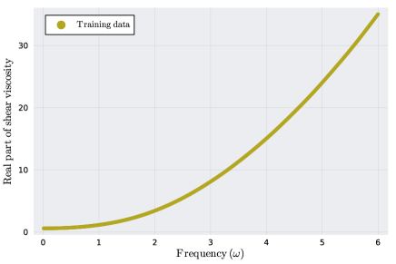
Figure 4: The real part of frequency-dependent shear viscosity in the LA model.

The training results are reported in Fig. 5, Fig. 8, and Tab. 1.

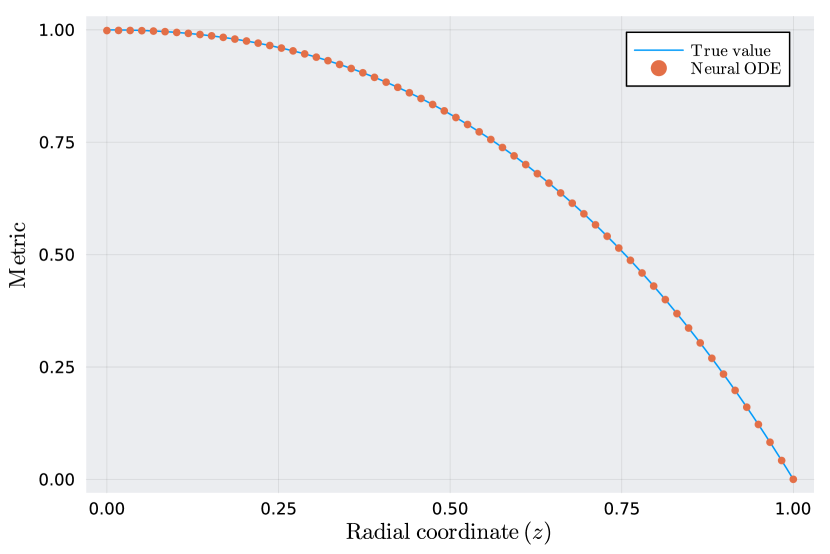
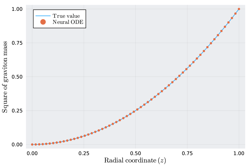
Figure 5: The performance of Neural ODEs for learning metric (left) and mass (right) in the LA model.

4.3 Generalized axions

In the above two models with broken translation symmetry, the mass square of the graviton has only one term. One may wonder if Neural ODEs can learn more general mass function. Here we will study the generalized axion (GA) model [60], which is a productive tool in the field of holographic condensed matters [61], see a recent application in amorphous solids [62]. Of particular interest to us, it can assign more general mass function to the graviton, while remaining analytically tractable.

Let’s generalize the bulk action (30) to the form

$$S_{\mathrm{bulk}}=\int d^{4}x\sqrt{-g}\left(\mathcal{R}+6-V(X)\right).$$ (39)

We will select the function $V(X)$ that has been used in [60]

$$V(X)=\gamma_{1}X+\gamma_{5}X^{5},$$ (40)

where $\gamma_{1}$ and $\gamma_{5}$ are two parameters. In terms of the holographic renormalization studied in [63], one can infer that the counterterms are the same as those in the LA model.

Taking the variation of the action, we can write down the equations of motion

$$R_{\mu\nu}-\frac{1}{2}g_{\mu\nu}R-3g_{\mu\nu} = X_{\mu\nu}V^{\prime}(X)-\frac{1}{2}g_{\mu\nu}V(X),$$ (41)

$$\nabla_{\mu}V^{\prime}\nabla^{\mu}\chi^{I}+V^{\prime}\nabla^{2}\chi^{I} = 0.$$ (42)

They have the analytical solution

$$f(z) = 1-z^{3}+\frac{1}{2}\sum_{n=1,5}\gamma_{n}\frac{z^{3}-z^{2n}}{3-2n},$$ (43)

$$\chi^{1} = x,\;\chi^{2}=y.$$ (44)

From the metric, we can read the temperature

$$T=\frac{1}{8\pi}\left(6-\sum_{n=1,5}\gamma_{n}\right).$$ (45)

We can also derive the graviton mass from Eq. (4) and

$$T_{\mu\nu}=2X_{\mu\nu}V^{\prime}(X)-g_{\mu\nu}V(X),$$ (46)

which yields

$$m^{2}=\sum_{n=1,5}n\gamma_{n}z^{2n}.$$ (47)

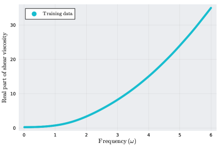
Figure 6: The real part of frequency-dependent shear viscosity in the GA model.

Using Eq. (43) and Eq. (47), the data are generated in Fig. 6. Here we have fixed the parameters $\gamma_{1}=\gamma_{5}=1$. We exhibit the training results in Fig. 7, Fig. 8, and Tab. 1.

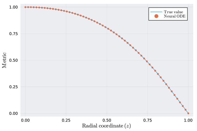
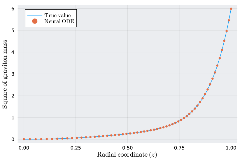
Figure 7: The performance of Neural ODEs for learning metric (left) and mass (right) in the GA model.

5 Conclusion and discussion

This work introduces an important physical ingredient in AdS/DL: translation symmetry breaking. Specifically, we extend the data-driven holographic transport model proposed in [34], allowing the machine to learn the black hole metric or the graviton mass from the real part of the shear viscosity. In addition, we use the Neural ODE to learn continuous functions, thereby avoiding the problem of discrete errors. These are the main physical and technical results of this work. Around them, we have the following comments.

1) Universality of theoretical framework

Although some assumptions still remain, the current theoretical framework, which mainly consists of the wave equation (3), the regularity at the horizon (7), and the boundary relation (8), is very general. Considering that the calculation of shear viscosity does not depend on the probe limit, this generality is quite rare.

2) Reconstruction of graviton mass

There are many ways to reconstruct the function of metric, but there has been no way to reconstruct the function of graviton mass before. Our work fills this gap, which may help to better understand the gravity dual of translation symmetry breaking in bottom-up holographic models.

3) At low temperatures

In Tab. 1, it is shown that the Neural ODE can achieve high accuracy for the bulk reconstruction. However, we caution that this is associated with the current model parameters ($\alpha,\beta,\gamma$), which are simply fixed to 1. As these parameters increase, the temperature of black holes decreases. Meanwhile, we observe a rapid degradation in the performance of Neural ODEs, although increasing the data can mitigate this trend. In the future, we expect to develop new machine learning techniques or introduce reasonable physical constraints to improve the performance of Neural ODEs at low temperatures.

4) Beyond AdS/CFT

The current theoretical framework necessitates the bulk spacetime to be asymptotic AdS. However, this information is not explicitly fed into the machine. Consequently, it would be plausible to construct more general data-driven holographic models, where the asymptotic geometry could be either Lifshitz or hyperscaling violated. Ultimately, the present work falls within the realm of reverse engineering of AdS/CFT, where the holographic dictionary is given a priori. One can also develop holographic machine learning that is independent of AdS/CFT [67, 64, 65, 66], which explores the emergence of spacetime and gravity from a more fundamental level.

Note added: Following the completion of this work, we became aware of Ref. [68], where the Neural ODE is used to learn the metric from the optical conductivity based on the linear axion model.

Appendix A From shear response to shear viscosity

Consider the bulk action of the Einstein gravity minimally coupled with the matter

$$S_{\mathrm{bulk}}=\int d^{4}x\sqrt{-g}\left(R+6+L_{\mathrm{matter}}\right),$$ (A.1)

and the wave equation of the shear mode

$$\frac{1}{\sqrt{-g}}\partial_{r}(\sqrt{-g}g^{rr}\partial_{r}h)+\left(\omega^{2}g^{tt}-m^{2}\right)h=0.$$ (A.2)

We require that the metric and graviton mass can be expanded near the AdS boundary, with the form

$$g_{tt} = r^{2}(1+\frac{a_{1}}{r}+\frac{a_{2}}{r^{2}}+\frac{a_{3}}{r^{3}}+\cdots),$$

$$g^{rr} = r^{2}(1+\frac{b_{1}}{r}+\frac{b_{2}}{r^{2}}+\frac{b_{3}}{r^{3}}+\cdots),$$

$$m^{2} = r^{-v}(c_{0}+\frac{c_{1}}{r}+\frac{c_{2}}{r^{2}}+\frac{c_{3}}{r^{3}}+\cdots),$$ (A.3)

where $\left(a_{i},b_{i},c_{i}\right)$ are some constants and $v$ is a positive integer.

Inserting Eq. (A.3) into Eq. (A.2), one can find that the asymptotic solution of the wave equation can be written as

$$h=h^{(0)}\left(1+d_{1}\frac{1}{r^{1}}+d_{2}\frac{1}{r^{2}}+d_{3}\frac{\log(r)}{r^{3}}\right)+h^{(3)}\frac{1}{r^{3}}+\cdots.$$ (A.4)

Here $h^{(0)}$ is the source, $h^{(3)}$ depends on $h^{(0)}$ and the incoming boundary condition on the horizon, and $d_{i}$ is determined by the frequency and the constants $a_{i}$, $b_{i}$, $c_{i}$ and $v$.

To ensure a well-defined variational system, we need the Gibbons-Hawking term and the counterterms

$$S_{\mathrm{GH}}=2\int d^{3}x\sqrt{-\gamma}K,\;S_{\mathrm{ct}}=\int d^{3}x\sqrt{-\gamma}\left(-4-R+L_{\mathrm{matter}}^{(1)}\right),$$ (A.5)

where $L_{\mathrm{matter}}^{(1)}$ denotes the counterterms contributed by the matter.

We expand the on-shell bulk action, the Gibbons-Hawking term, and the counterterms to the second order of the shear mode,

$$\left.S_{\mathrm{bulk}}+S_{\mathrm{GH}}+S_{\mathrm{ct}}\right|_{\mathrm{on-shell}}=\int d^{2}x\int_{-\infty}^{\infty}\frac{d\omega}{2\pi}\frac{1}{2}\left[\left(L_{\mathrm{gravity}}^{(2)}+L_{\mathrm{matter}}^{(2)}\right)\bar{h}h-r^{2}\sqrt{\frac{g_{tt}}{g_{rr}}}\bar{h}h^{\prime}\right],$$ (A.6)

where $\bar{h}$ has the argument $-\omega$. In the terms $\sim\bar{h}h$, $L_{\mathrm{gravity}}^{(2)}$ can be referred as the gravity contribution and $L_{\mathrm{matter}}^{(2)}$ denotes the contribution from $L_{\mathrm{matter}}^{(1)}$. We find that the former has a universal expression

$$L_{\mathrm{gravity}}^{(2)}=-\frac{r^{2}\omega^{2}}{\sqrt{g_{tt}}}+4r^{2}\sqrt{g_{tt}}-2r\sqrt{\frac{g_{tt}}{g_{rr}}}-\frac{r^{2}g_{tt}^{\prime}}{\sqrt{g_{tt}g_{rr}}},$$ (A.7)

while both $L_{\mathrm{gravity}}^{(2)}$ and $L_{\mathrm{matter}}^{(2)}$ generally diverge at the boundary.

Inputting Eq. (A.3) and Eq. (A.4) into Eq. (A.6), we obtain the renormalized action

$$S_{\mathrm{ren}}=\int d^{2}x\int_{-\infty}^{\infty}\frac{d\omega}{2\pi}\frac{1}{2}\left[\left(L_{\mathrm{gravity}}^{(3)}+L_{\mathrm{matter}}^{(3)}\right)\bar{h}^{(0)}h^{(0)}+3\bar{h}^{(0)}h^{(3)}\right],$$ (A.8)

where $L_{\mathrm{gravity}}^{(3)}$ and $L_{\mathrm{matter}}^{(3)}$ are finite and they are contributed by the gravity and the matter, respectively. One can find that $L_{\mathrm{gravity}}^{(3)}$ is real since it is composed of the real constants in Eq. (A.3). We also argue that $L_{\mathrm{matter}}^{(3)}$ is usually real. This is based on the following facts and assumptions.

1) The counterterms should be the intrinsic scalars defined on the boundary.

2) The induced metric has no $\gamma^{tx}$ and $\gamma^{ty}$ components on the background level.

3) All other fields coupled to $\gamma_{xy}$ are supposed to be time-independent.

4) The gauge symmetry should be respected.

5) The system is supposed to be rotationally invariant.

Using 1)-3), one can see that $L_{\mathrm{matter}}^{(3)}$ cannot have an imaginary part unless the expansion of $L_{\mathrm{matter}}^{(1)}$ contains a term

$$L_{\mathrm{im}}\sim\gamma^{tt}\partial_{t}\gamma_{xy}\gamma_{xy}\left(A,\partial A\right)_{t\cdots},$$ (A.9)

where $\left(A,\partial A\right)_{t\cdots}$ denotes certain matter field or its spatial derivative with the indices $t\cdots$. The expression of $L_{\mathrm{im}}$ is understood that the subscript $t$ in $\partial_{t}\gamma_{xy}$ must be paired with the subscript $t$ in $\left(A,\partial A\right)_{t\cdots}$ in order to contract with the superscripts of $g^{tt}$. Obviously, $A$ is neither a scalar nor a spinor since they have no spacetime indices. $A$ is not a U(1) vector if 4)-5) are taken into account further. Thus, there is no such term at least in any Einstein-Maxwell-Dirac-scalar models.

To proceed, we extract the retarded correlator from $S_{\mathrm{ren}}$:

$$G_{T^{xy}T^{xy}}^{R}(\omega)=L^{(3)}+3\frac{h^{(3)}}{h^{(0)}},$$ (A.10)

where $L^{(3)}=L_{\mathrm{gravity}}^{(3)}+L_{\mathrm{matter}}^{(3)}$. Expand the response function near the boundary, which yields

$$\left.\chi(\omega)\right|_{r\rightarrow\infty}=\left.\frac{\Pi}{i\omega h}\right|_{r\rightarrow\infty}=\left.-\frac{\sqrt{-g}g^{rr}\partial_{r}h}{i\omega h}\right|_{r\rightarrow\infty}=\frac{1}{i\omega}\left.\left(\frac{3h^{(3)}}{h^{(0)}}-e_{1}\right)\right|_{r\rightarrow\infty}.$$ (A.11)

Here $e_{1}$ is real, relying on $r$, $\omega$, and previous constants. Comparing Eq. (A.10) and Eq. (A.11), we have

$$\left.\chi(\omega)\right|_{r\rightarrow\infty}=\frac{1}{i\omega}G_{T^{xy}T^{xy}}^{R}(\omega)-\frac{1}{i\omega}\left.\left(L^{(3)}+e_{1}\right)\right|_{r\rightarrow\infty}.$$ (A.12)

Importantly, the last term of Eq. (A.12), which depends on the UV details of specific models, is imaginary.

In view of this, we will consider the Kubo formula for the real part of the frequency-dependent shear viscosity [69, 70, 34]

$$\eta_{\mathrm{re}}(\omega)=\frac{1}{\omega}\mathrm{Im}\left[G_{T^{xy}T^{xy}}^{R}(\omega)\right].$$ (A.13)

Combining Eq. (A.12) and Eq. (A.13), we finally obtain a simple equality between the shear viscosity and the shear response

$$\eta_{\mathrm{re}}(\omega)=\left.\chi_{\mathrm{re}}(\omega)\right|_{r\rightarrow\infty}.$$ (A.14)

Appendix B Training scheme and report

In order to perform training, we need to make some settings.

1) Neural network

We use a neural network to represent the metric or mass. It is a fully connected feed-forward network consisting of three dense layers:

$$(1,5)\rightarrow(5,5,\mathrm{tanh})\rightarrow(5,1).$$ (A.15)

For each layer, we have specified the number of input nodes and output nodes. In the second layer, a tanh activation is used. Note that the neural network has 46 trainable parameters, which include weights and biases.

2) ODE solver

Our Neural ODEs are solved using the Tsitouras 5/4 Runge-Kutta method [71].

3) IR and UV cutoffs

In solving the ODEs numerically, the horizon and boundary cannot be touched exactly. We set the IR and UV cutoffs as $z_{\mathrm{IR}}=0.9999$ and $z_{\mathrm{UV}}=0.0001$.

4) Initial values

To learn the metric, the neural network is initialized by sampling from a standard normal distribution $N(0,1)$. The normal distribution $N(0,0.001)$ with a small standard deviation is utilized for learning the mass and hyperparameter tuning.

5) Hyperparameter tuning

There are various hyperparameter tuning methods, which consume different computing resources. Here we propose a simple way to quickly find the exponent $b$ in the square of graviton mass. We define the search range as $[0,4]$ with the step size 1. We use the standard cross-validation method with the simple hold-out technique [72]. We separate the dataset with the frequency range $[0.01,\omega_{\max}]$ into two parts. The part with $[0.01,\omega_{\max}-1]$ goes to the training set and the part with $[\omega_{\max}-0.99,\omega_{\max}]$ to the validation set. The rationale for this separation lies in the dependence of the exponent $b$ on the UV physics. We use the optimizers RMSProp and Adam in order. Their learning rates, epoch numbers, and batch sizes are set as (0.001, 0.0001), (10, 10) and (1, 1). We also add the L1 regularization term $L_{1}=0.1\times\left|\theta\right|$ in the loss function. For each $b$ in the search range, we train 5 times and take the average validation error to select the optimal $b$. As long as $\omega_{\max}$ is large enough, the correct $b$ can be found for the current three targets. Specifically, $\omega_{\max}=2$ is large enough for the MG and LA models, and $\omega_{\max}=4$ is large enough for the GA model, see Fig. 8.

6) Training process

The training process can be divided into four stages, which are described as follows.

a) In most cases, the optimizers (RMSProp, Adam, Adam, BFGS) are used sequentially in four stages. For learning the mass of the MG and the LA models, only the first two training stages are needed, as the log-cosh loss becomes negligible (less than the machine epsilon $\sim 1\times 10^{-16}$).

b) The learning rates (0.001, 0.0001, 0.00001) are used sequentially in first three stages. The epoch numbers are (10, 10, 100) respectively. The batch sizes are all set as 1. In the fourth stage, the initial size of the step is set as 0.01 and the maximum number of iterations is set as 500.

c) In the first stage, we train $T_{1}=120$ times, each time with randomly initialized trainable parameters. In the $i$-th stage with $i>1$, we obtain the initial parameters from the top $T_{i}=T_{i-1}/2$ trained results with the minimum loss in the $\left(i-1\right)$-th stage. We conduct parallel training on multiple computer cores. When more than $T_{i}/2$ tasks are completed, we stop the $i$-th stage and move on to the $\left(i+1\right)$-th stage. This early stopping can effectively prevent the machine from getting stuck in solving Neural ODEs with bad parameters.

After training, we collect information on the best result, including the minimum loss, the MRE of the learned metric, and the MRE of the learned mass square, see Tab. 1.

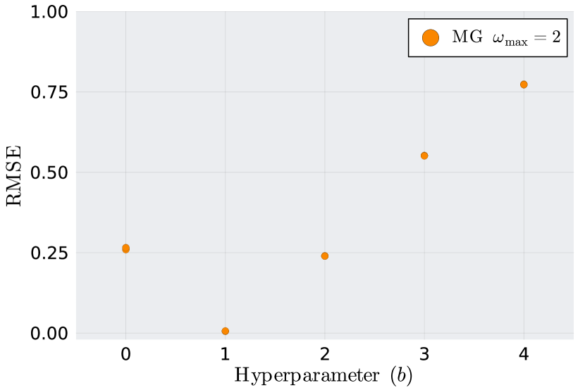
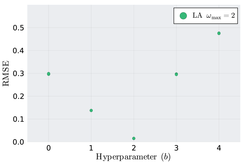
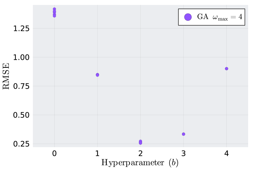
Figure 8: Root mean square error (RMSE) for evaluating the hyperparameter $b$ in MG (left), LA (middle) and GA (right) models. Each $b$ is trained five times, yielding five nearly coincident RMSE points in most cases. As one can see, the optimal hyperparameters for three models are 1, 2, and 2, respectively.

Target	$f$ of MG	$m^{2}$ of MG	$f$ of LA	$m^{2}$ of LA	$f$ of GA	$m^{2}$ of GA
Loss	$7\times 10^{-10}$	$<1\times 10^{-16}$	$2\times 10^{-10}$	$<1\times 10^{-16}$	$6\times 10^{-10}$	$1\times 10^{-11}$
MRE	$5\times 10^{-5}$	$3\times 10^{-9}$	$1\times 10^{-5}$	$2\times 10^{-10}$	$7\times 10^{-5}$	$6\times 10^{-4}$

Table 1: Minimum loss and MRE of six machine learning experiments. Their learning targets are the metric and mass square in the models of MG, LA and GA.

References

- [1] O. Aharony, S. S. Gubser, J. Maldacena, H. Ooguri and Y. Oz, Large N Field Theories, String Theory and Gravity, Phys. Rep. 323, 183 (2000). [arXiv:hep-th/9905111].
- [2] H. Liu and J. Sonner, Quantum many-body physics from a gravitational lens, Nature Rev. Phys. 2, 615 (2020). [arXiv:2004.06159].
- [3] T. De Jonckheere, Modave lectures on bulk reconstruction in AdS/CFT, PoS Modave2017 005 (2018). [arXiv:1711.07787].
- [4] D. Harlow, TASI Lectures on the emergence of bulk physics in AdS/CFT, PoS TASI2017 002 (2018). [arXiv:1802.01040].
- [5] N. Kajuri, Lectures on bulk reconstruction, SciPost Phys. Lect. Notes 22 (2021). [arXiv:2003.00587].
- [6] S. de Haro, S. N. Solodukhin and K. Skenderis, Holographic reconstruction of space-time and renormalization in the AdS/CFT correspondence, Commun. Math. Phys. 217, 595 (2001). [arXiv:hep-th/0002230].
- [7] J. Hammersley, Extracting the bulk metric from boundary information in asymptotically AdS spacetimes, JHEP 12, 047 (2006). [arXiv:hep-th/0609202].
- [8] V. E. Hubeny, H. Liu and M. Rangamani, Bulk-cone singularities & signatures of horizon formation in AdS/CFT, JHEP 01, 009 (2007). [arXiv:hep-th/0610041].
- [9] J. Hammersley, Numerical metric extraction in AdS/CFT, Gen. Rel. Grav. 40, 1619 (2008). [arXiv:0705.0159].
- [10] S. Bilson, Extracting spacetimes using the AdS/CFT conjecture, JHEP 08, 073 (2008). [arXiv:0807.3695].
- [11] S. Bilson, Extracting Spacetimes using the AdS/CFT Conjecture: Part II, JHEP 02, 050 (2011). [arXiv:1012.1812].
- [12] V. E. Hubeny, Extremal surfaces as bulk probes in AdS/CFT, JHEP 07, 093 (2012). [arXiv:1203.1044].
- [13] V. Balasubramanian, B. D. Chowdhury, B. Czech, J. de Boer and M. P. Heller, Bulk curves from boundary data in holography, Phys. Rev. D 89, 086004 (2014). [arXiv:1310.4204].
- [14] R. C. Myers, J. Rao and S. Sugishita, Holographic Holes in Higher Dimensions, JHEP 06, 044 (2014). [arXiv:1403.3416].
- [15] B. Czech and L. Lamprou, Holographic definition of points and distances, Phys. Rev. D 90, 106005 (2014). [arXiv:1409.4473].
- [16] N. Engelhardt and G. T. Horowitz, Towards a Reconstruction of General Bulk Metrics, Class. Quant. Grav. 34, 015004 (2017). [arXiv:1605.01070].
- [17] N. Engelhardt and G. T. Horowitz, Recovering the spacetime metric from a holographic dual, Adv. Theor. Math. Phys. 21, 1635 (2017). [arXiv:1612.00391].
- [18] S. R. Roy and D. Sarkar, Bulk metric reconstruction from boundary entanglement, Phys. Rev. D 98, 066017 (2018). [arXiv:1801.07280].
- [19] D. Kabat and G. Lifschytz, Emergence of spacetime from the algebra of total modular Hamiltonians, JHEP 05, 017 (2019). [arXiv:1812.02915].
- [20] K. Hashimoto, Building bulk from Wilson loops, PTEP 2021, 023B04 (2021). [arXiv:2008.10883].
- [21] K. Hashimoto and R. Watanabe, Bulk reconstruction of metrics inside black holes by complexity, JHEP 09, 165 (2021). [arXiv:2103.13186].
- [22] S. Caron-Huot, Holographic cameras: An eye for the bulk, JHEP 03, 047 (2023). [arXiv:2211.11791].
- [23] N. Jokela, A. Pönni, T. Rindlisbacher, K. Rummukainen and A. Salami, Disentangling the gravity dual of Yang-Mills theory, JHEP 12, 137 (2023). [arXiv:2304.08949].
- [24] W. B. Xu and S. F. Wu, Reconstructing black hole exteriors and interiors using entanglement and complexity, JHEP 07, 083 (2023). [arXiv:2305.01330].
- [25] T. M. Nebabu and X. Qi, Bulk Reconstruction from Generalized Free Fields, arXiv:2306.16687.
- [26] R. Q. Yang, Inverse problem of correlation functions in holography and bulk reconstruction, arXiv:2310.10419.
- [27] K. Hashimoto, S. Sugishita, A. Tanaka and A. Tomiya, Deep learning and the AdS/CFT correspondence, Phys. Rev. D 98, 046019 (2018). [arXiv:1802.08313].
- [28] K. Hashimoto, S. Sugishita, A. Tanaka and A. Tomiya, Deep Learning and Holographic QCD, Phys. Rev. D 98, 106014 (2018). [arXiv:1809.10536].
- [29] T. Akutagawa, K. Hashimoto and T. Sumimoto, Deep Learning and AdS/QCD, Phys. Rev. D 102, 026020 (2020). [arXiv:2005.02636].
- [30] K. Hashimoto, H. Y. Hu and Y. Z. You, Neural ordinary differential equation and holographic quantum chromodynamics, Mach. Learn.: Sci. Technol. 2, 035011 (2021). [arXiv:2006.00712].
- [31] K. Hashimoto, K. Ohashi and T. Sumimoto, Deriving the dilaton potential in improved holographic QCD from the meson spectrum, Phys. Rev. D 105, 106008 (2022). [arXiv:2108.08091].
- [32] R. Katsube, W. H. Tam, M. Hotta and Y. Nambu, Deep learning metric detectors in general relativity, Phys. Rev. D 106, 044051 (2022). [arXiv:2206.03006].
- [33] K. Hashimoto, K. Ohashi and T. Sumimoto, Deriving dilaton potential in improved holographic QCD from chiral condensate, PTEP 2023, 033B01 (2023). [arXiv:2209.04638].
- [34] Y. K. Yan, S. F. Wu, X. H. Ge and Y. Tian, Deep learning black hole metrics from shear viscosity, Phys. Rev. D 102, 101902(R) (2020). [arXiv:2004.12112].
- [35] K. Li, Y. Ling, P. Liu and M. H. Wu, Learning the black hole metric from holographic conductivity, Phys. Rev. D 107, 066021 (2023). [arXiv:2209.05203].
- [36] K. Hashimoto, H. Y. Hu and Y. Z. You, Neural ODE and Holographic QCD, Mach. Learn.: Sci. Technol 2, 035011 (2021). [arXiv:2006.00712].
- [37] Ricky T. Q. Chen, Y. Rubanova, J. Bettencourt and D. Duvenaud. Neural Ordinary Differential Equations. In: Advances in Neural Information Processing Systems 31 (NeurIPS 2018). [arXiv:1806.07366].
- [38] K. Skenderis, Lecture notes on holographic renormalization, Class. Quantum. Gravity 19, 5849 (2002). [arXiv:hep-th/0209067].
- [39] I. Papadimitriou, Lectures on Holographic Renormalization, Springer Proceedings in Physics Vol. 176: Theoretical Frontiers in Black Holes and Cosmology, Springer Press (2016).
- [40] S. A. Hartnoll, D. M. Ramirez and J. E. Santos, Entropy production, viscosity bounds and bumpy black holes, JHEP 03, 170 (2016). [arXiv:1601.02757].
- [41] J. Zaanen, Y. Liu, Y. W. Sun and K. Schalm, Holographic Duality in Condensed Matter, Chapter 12, Cambridge University Press (2015).
- [42] K. M. He, X. Y. Zhang, S. Q. Ren and J. Sun. Deep Residual Learning for Image Recognition. In: 2016 IEEE Conference on Computer Vision and Pattern Recognition (CVPR) 770 (2016). [arXiv:1512.03385].
- [43] L. S. Pontryagin, E. F. Mishchenko, V. G. Boltyanskii and R. V. Gamkrelidze, The mathematical theory of optimal processes, 1962.
- [44] P. F. Chen, G. Y. Chen and S. Y. Zhang, Log Hyperbolic Cosine Loss Improves Variational Auto-Encoder, 2018.
- [45] Q. Wang, Y. Ma, K. Zhao and Y. J. Tian, A Comprehensive Survey of Loss Functions in Machine Learning, Ann. Data. Sci. 9, 187 (2020).
- [46] X. Xu, J. Li, Y. Yang and F. M. Shen, Toward Effective Intrusion Detection Using Log-Cosh Conditional Variational Autoencoder, IEEE Internet of Things Journal 8, 6187 (2021).
- [47] Resve A. Saleh and A. K. Md. Ehsanes Saleh, Statistical Properties of the log-cosh Loss Function Used in Machine Learning, [arXiv:2208.04564].
- [48] Jorge Nocedal and Stephen J. Wright. Quasi-Newton Methods. In: Numerical Optimization 135, 3 Springer New York (2006).
- [49] M. Fierz and W. Pauli, On Relativistic Wave Equations for Particles of Arbitrary Spin in an Electromagnetic Field, Proc. Roy. Soc. Lond. 173, 211 (1939).
- [50] H. van Dam and M. J. Veltman, Massive and mass-less Yang-Mills and gravitational fields, Nucl. Phys. B 22, 397 (1970).
- [51] V. I. Zakharov, Linearized Gravitation Theory and the Graviton Mass, JETP Lett. 12, 312 (1970).
- [52] A. I. Vainshtein, To the problem of nonvanishing gravitation mass, Phys. Lett. B 39, 393 (1972).
- [53] D. G. Boulware and S. Deser, Can Gravitation Have a Finite Range? Phys. Rev. D 6, 3368 (1972).
- [54] D. Vegh, Holography without translational symmetry, [arXiv:1301.0537].
- [55] C. de Rham and G. Gabadadze, Generalization of the Fierz-Pauli Action, Phys. Rev. D 82, 044020 (2010). [arXiv:1007.0443].
- [56] C. de Rham, G. Gabadadze and A. J. Tolley, Resummation of Massive Gravity, Phys. Rev. Lett. 106, 231101 (2011). [arXiv:1011.1232].
- [57] C. de Rham, Massive Gravity, Living Rev. Relativity 17, 7 (2014). [arXiv:1401.4173].
- [58] F. Chen, S. F. Wu and Y. X. Peng, Hamilton-Jacobi Approach to Holographic Renormalization of Massive Gravity, JHEP 07, 072 (2019). [arXiv:1903.02672].
- [59] T. Andrade and B. Withers, A simple holographic model of momentum relaxation, JHEP 05, 101 (2014). [arXiv:1311.5157].
- [60] M. Baggioli and O. Pujolas, Holographic Polarons, the Metal-Insulator Transition and Massive Gravity, Phys. Rev. Lett. 114, 251602 (2015). [arXiv:1411.1003].
- [61] M. Baggioli, K. Y. Kim, L. Li and W. J. Li, Holographic Axion Model: a simple gravitational tool for quantum matter, Sci. China Phys. Mech. Astron. 64, 270001 (2021). [arXiv:2101.01892].
- [62] D. Pan, T. Ji, M. Baggioli, L. Li and Y. Jin, Non-linear elasticity, yielding and entropy in amorphous solids, Sci. Adv. 8, eabm8028 (2022). [arXiv:2108.13124].
- [63] M. X. Ma and S. F. Wu, Holographic renormalization in the Hamilton-Jacobi formulation with exact ansatz generation, Phys. Rev. D 107, 066012 (2023). [arXiv:2208.10012].
- [64] H. Y. Hu, S. H. Li, L. Wang and Y. Z. You, Machine Learning Holographic Mapping by Neural Network Renormalization Group, Phys. Rev. Res. 2, 023369 (2020). [arXiv:1903.00804].
- [65] X. Han and S. A. Hartnoll, Deep Quantum Geometry of Matrices, Phys. Rev. X 10, 011069 (2020). [arXiv:1906.08781].
- [66] J. Lam and Y. Z. You, Machine learning statistical gravity from multi-region entanglement entropy, Phys. Rev. Res. 3, 043199 (2021). [arXiv:2110.01115].
- [67] Y. Z. You, Z. Yang and X. L. Qi, Machine Learning Spatial Geometry from Entanglement Features, Phys. Rev. B 97, 045153 (2018). [arXiv:1709.01223].
- [68] B. Ahn, H. S. Jeong, K. Y. Kim and K. Yun, Deep learning bulk spacetime from boundary optical conductivity, [arXiv:2401.00939].
- [69] B. Bradlyn, M. Goldstein and N. Read, Kubo formulas for viscosity: Hall viscosity, Ward identities, and the relation with conductivity, Phys. Rev. B 86, 245309 (2012). [arXiv:1207.7021].
- [70] M. Geracie, D. T. Son, C. Wu and S. F. Wu, Spacetime Symmetries of the Quantum Hall Effect, Phys. Rev. D 91, 045030 (2015). [arXiv:1407.1252].
- [71] C. Tsitouras, Runge-Kutta pairs of orders 5(4) satisfying only the first column simplifying assumption, Computers and Mathematics with Applications 62, 770 (2011).
- [72] S. Arlot and A. Celisse, A survey of cross-validation procedures for model selection, Statistics Surveys 4, 40 (2010). [arXiv:0907.4728].