Infinite-Horizon Graph Filters: Leveraging Power Series
to Enhance Sparse Information Aggregation

Abstract

Graph Neural Networks (GNNs) have shown considerable effectiveness in a variety of graph learning tasks, particularly those based on the message-passing approach in recent years. However, their performance is often constrained by a limited receptive field, a challenge that becomes more acute in the presence of sparse graphs. In light of the power series, which possesses infinite expansion capabilities, we propose a novel Graph Power Filter Neural Network (GPFN) that enhances node classification by employing a power series graph filter to augment the receptive field. Concretely, our GPFN designs a new way to build a graph filter with an infinite receptive field based on the convergence power series, which can be analyzed in the spectral and spatial domains. Besides, we theoretically prove that our GPFN is a general framework that can integrate any power series and capture long-range dependencies. Finally, experimental results on three datasets demonstrate the superiority of our GPFN over state-of-the-art baselines.

1 Introduction

Graph neural networks (GNNs) have attracted significant attention in the research community due to their exceptional performance in a variety of graph learning applications, including social analysis Qin et al. (2022); Matsugu et al. (2023) and traffic forecasting Li et al. (2022); Gao et al. (2023); Jiang et al. (2023); Fang et al. (2023). A prevalent method involves the use of message-passing Kipf and Welling (2016); Hamilton et al. (2017) technique to manage node features and the topology of the graph. Various layer types Xu et al. (2019); Defferrard et al. (2016) like graph convolutional (GCN)  Kipf and Welling (2016) and graph attention layers (GAT) Veličković et al. (2018) enable GNNs to capture complex relationships, enhancing their performance across multiple domains. However, despite their advancements in graph representation learning, message-passing-based GNNs still face certain limitations.

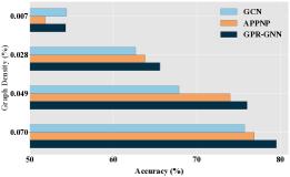
Figure 1: The influence of GCN Kipf and Welling (2016), APPNP Gasteiger et al. (2022), and GPR-GNN Eli Chien and Milenkovic (2021) on the node classification task under different sparse situations.

i) Long-range Dependencies: Balancing the trade-off between the receptive field size and feature distinctiveness is a challenging aspect in GNNs. On the one hand, deeper GNNs Eli Chien and Milenkovic (2021); Li et al. (2019); He et al. (2021) offer a larger receptive field, which allows for the incorporation of information from a broader range of the graph. However, this comes with the downside of feature homogenization across nodes, leading to the phenomenon known as over-smoothing. On the other hand, GNNs with shallower structures Rusch et al. (2023), while avoiding over-smoothing, face limitations in capturing long-range dependencies due to their smaller receptive field. This limitation is particularly significant in real-world graphs, such as social networks or protein interaction networks, where understanding distant node relationships is crucial. ii) Graph Sparsity: A sparse graph is a type of graph in which the number of edges is relatively low compared to the total number of possible edges. Such graphs are common in real-world scenarios. For instance, Berger et al. (2005); Ahad N. et al. (2023) reveals that the degree distribution of real-world graphs typically follows a power-law distribution. In particular, the citation network-based Cora and Citeseer datasets exhibit remarkable levels of sparsity, measured at 99.93% and 99.96%, respectively. Because sparse graphs contain less explicit information due to fewer edges, it is hard to mine effective representations, even for contemporary GNNs. As shown in Figure 1, as the number of edges decreases gradually, the performance of GNNs drops correspondingly, indicating that learning effective representations on sparse graphs remains an unresolved challenge.

In this paper, we endeavor to address the challenges previously mentioned by explicitly modeling dependencies over an infinite range within a single layer. This strategy effectively harnesses valuable information in sparse graphs and captures long-range dependencies without incurring the over-smoothing issue. Specifically, inspired by the impressive capability of power series for infinite expansion, we propose a novel method named Graph Power Filter Neural Network (GPFN). A noteworthy point is that employing a standard power series graph filter can lead to a substantial computational burden. Existing approaches, such as BernNet He et al. (2021), opt to truncate the K-order polynomial to simplify the complexity, but these methods might lose long-range information. In contrast, GPFN is designed to construct the graph filter using convergent power series from the spectral domain. This approach ensures the preservation of the infinite modeling capability of power series without information loss. We substantiate the effectiveness of our proposed GPFN with both theoretical and empirical evidence.

In summary, our contributions are listed as follows:

• Our proposed framework GPFN utilizes convergent infinite power series derived from the spectral domain for aggregating long-range information, which significantly mitigates the adverse impacts associated with graph sparsity.

• We analyze GPFN from a spatial domain perspective, focusing on its ability to effectively capture long-range dependencies. Additionally, we provide theoretical evidence demonstrating that our GPFN is not only capable of achieving exceptional performance using shallow layers but also effectively integrates various power series.

• We validate our GPFN through experiments on three real-world graph datasets, tested across various sparse graph settings. The experimental results demonstrate the advantages of our GPFN over state-of-the-art baselines, especially in contexts of extreme graph sparsity.

2 Related Work

Monomial graph filters.

These filters are mainly aimed at filtering information between two layers, without introducing more layer parameters. Spectral GNNs are grounded in the concept of the graph Fourier filter, as introduced by Ortega et al. (2018); Monti et al. (2016), wherein the eigenbasis of the graph Laplacian is analogously employed. Subsequently, GCN Kipf and Welling (2016) substitutes the convolutional core with first-order Chebyshev approximation. Other monomeric graph filters are GAT Veličković et al. (2018), GIN Xu et al. (2019), AGE Cui et al. (2020) and SGC Wu et al. (2019).

Polynomial graph filters.

Polynomial filters encompass ResGCN Li et al. (2019), BernNet He et al. (2021), and GPR-GNN Eli Chien and Milenkovic (2021), etc.. ResGCN employs residual connections to facilitate information transfer between different layers, alleviating the over-smoothing issues. However, ResGCN focuses more on intermediate information, neglecting the significance of proximal information. BernNet utilizes Bernstein polynomials to aggregate information across different layers. Nevertheless, due to layer constraints, BernNet struggles to extend its reach to more distant information, and parameter learning becomes more challenging. APPNP Gasteiger et al. (2022) and GRAND Feng et al. (2022) utilize feature propagation but within a limited number of hops. GPR-GNN unifies the representation of parameters between different layers in a general polynomial formula, therefore APPNP, ResGCN and BernNet can all be regarded as special case of GPR-GNN. However, GPR-GNN requires learning relative control parameters between layers. Similar to BernNet, the receptive field of view is limited, and parameter learning poses a significant challenge.

3 Preliminaries

3.1 Problem Formulation

Definition 1. (Sparse graph)

Given a graph $\mathcal{G}=(\mathcal{V,E,Y},A,X)$, $\mathcal{V}=\{v_{1},\cdots,v_{N}\}$ is the set of nodes, and $\mathcal{E}\subseteq\mathcal{V}\times\mathcal{V}$ is the edge set. $\mathcal{Y}$ is the set of labels for node in $\mathcal{V}$. $A\in\mathbb{R}^{N\times N}$ denotes the adjacency matrix, where $A_{ij}>0$ if $(v_{i},v_{j})\in\mathcal{E}$ and $A_{ij}=0$ if $(v_{i},v_{j})\notin\mathcal{E}$. $X\in\mathbb{R}^{N\times D}$ is the attribute matrix, and $D$ is the number of attribute dimensions. If there exists $|\mathcal{E}|\ll|\mathcal{V}^{2}|$, we call $\mathcal{G}$ a sparse graph.

Definition 2. (Label prediction for sparse graph)

Given a sparse graph $\mathcal{G}=(\mathcal{V,E,Y},A,X)$, and the node set is divided into a train set and a test set, i.e., $\mathcal{V}=\mathcal{V}_{\rm{train}}\cup\mathcal{V}_{\rm{test}}$. The label $y_{i}$ of node $v_{i}$ can be observed only if $v_{i}\in\mathcal{V}_{\rm{train}}$. The goal of label prediction is to predict test labels $\mathcal{Y}_{\rm{test}}=\{y_{i}|v_{i}\in\mathcal{V}_{\rm{test}}\}$. We utilize a two-layer GNN for downstream tasks and predict the label $\hat{Y}$ as $\hat{Y}=\text{GNN}(X,A)$. And the surprised Cross-Entropy Loss function is:$\quad\min_{\rho}L_{pre}=\frac{1}{N}\sum_{i}\sum_{c=1}^{|Y|}-y_{ic}\log(\hat{y}_{ic}),$ here $|Y|$ is the number of classes, and $y_{ic}$ is 1 if node $v_{i}$ belongs to class $c$, else it is 0. $\hat{y}_{ic}$ is the predicted probability that node $v_{i}$ belongs to class $c$. $\rho$ is the parameter of the GNN predictor.

3.2 Revisiting Graph Neural Networks

We revisiting GNNs from two perspectives:

(Spatial Domain)

The message passing-based GCN Kipf and Welling (2016) can be formed as follows:

$$\footnotesize H^{(0)}=X,\quad H^{(l+1)}=\sigma(\hat{A}H^{(l)}W^{(l)}),$$ (1)

where $\hat{A}$ is the aggregation matrix. Particularly, $\tilde{A}_{sym}=\tilde{D}^{-\frac{1}{2}}\tilde{A}\tilde{D}^{-\frac{1}{2}}$, where $\tilde{A}=A\,+\,I$ and $\tilde{D}$ are the adjacency matrix with the identity matrix-based self-loop and the degree matrix of $\tilde{A}$. $H^{(l)}\in\mathbb{R}^{N\times D}$ is the node representation matrix at $l$-th layer and $\sigma(\cdot)$ denotes an activation function.

(Spectral Domain)

The spectral convolution Shuman et al. (2013) of attribute $X$ and filter $F_{\gamma}$ can be formulated as:

$$\footnotesize F_{\gamma}*X=U\bigl{(}(U^{T}F_{\gamma})\odot(U^{T}X)\bigl{)}=UF_{\gamma}(\Lambda)U^{T}X,$$ (2)

where $*$ is graph convolution and $\odot$ is Hadamard product. Note that the decomposition of aggregation matrix$\hat{A}=U\Lambda U^{T}$ can be used to obtain eigenvectors as Fourier bases and eigenvalues as frequencies.

3.3 Eigenvalue of Aggregation Matrix

Previous studies Cui et al. (2020) reveal that the Rayleigh Quotient can be used to calculate the lower bound and upper bound of eigenvalues of $\hat{A}$, that is $\lambda_{min}=\min(R)\leq\max(R)=\lambda_{max}$ Cui et al. (2020). Thus, for node $v_{i}$, its Rayleigh Quotient is $R(\hat{A},u_{i})=\lambda_{i}$, and we let $q_{i}=\widetilde{D}^{-1/2}u_{i}$, where $U=\text{diag}(u_{1},\ldots,u_{n})$ is eigenvalue decomposition of $\hat{A}$. Because $R(\widetilde{L}_{sym},u_{i})$ is a division of two quadratic forms, the eigenvalues are non-negative. We prove that the maximum of $\widetilde{L}_{sym}$ eigenvalue is $2$ iff the graph is bipartite as shown in Appendix A. Therefore, for $\widetilde{L}_{sym}=I+\tilde{A}_{sym}$, the eigenvalues of the $\tilde{A}_{sym}$ satisfy the following equation: $1=\lambda_{1}\geq\lambda_{2}\geq\cdots\geq\lambda_{N}>-1$, as previous study reveals Luxburg (2007).

4 Methodology

In this section, we detail our proposed GPFN. Initially, in Section 4.1, we elucidate the methodology for designing a graph filter based on a power series. Subsequently, in Sections 4.2 and 4.3, we introduce three fundamental power series filters and substantiate their effectiveness as well as the rationale behind the choice of hyperparameters $\beta_{0}$. Ultimately, we juxtapose and analyze the relations between our Power Series Filters and the preceding research. In general, there are two perspectives as shown in Figure 2 – spectral and spatial domains to support the analysis of Power Series Filters:

• (Spectral Domain) A flexible graph filter framework. We demonstrate that a variety of filter types, such as low-pass, high-pass, or band-pass, can be conveniently devised by simply adjusting the filter coefficients $\gamma_{n}$ (refer to Section 4.1). Furthermore, we exhibit that other polynomial filters can be induced into our framework, thereby affirming its extensive applicability and adaptability.

• (Spatial Domain) An infinite information aggregator. Filters constructed via power series possess the capability to aggregate neighborhood information across an infinite number of hops with variant weights, thereby enlarging the graph’s receptive field.

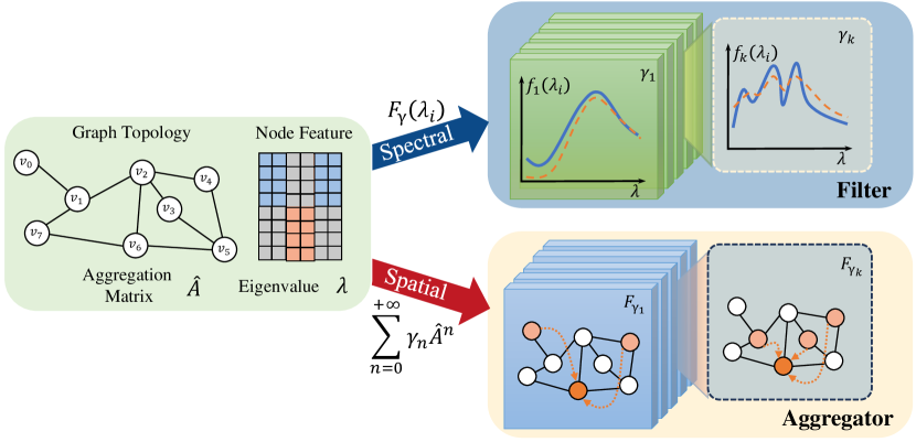
Figure 2: The overall framework of GPFN. For arbitrary power series over the aggregation matrix, we can design corresponding filters in the spectral domain, which also serve as an infinite aggregator in the spatial domain.

4.1 Generalized Filter

4.1.1 Foundation of Power Series

To grasp the fundamentals of GPFN, it is essential to review the concept of power series. In mathematics, a power series, exemplified here as a single variable, is an infinite series of the standard form:

$$\footnotesize\sum_{n=0}^{+\infty}a_{n}x^{n}=a_{0}+a_{1}x+\cdots+a_{i}x^{i}+\cdots,$$ (3)

where $i\in\mathbb{N}^{+}$, $a_{n}$ represents the coefficient of the $n$-th term. When this power series converges and variable $x$ is constrained within the convergence region $[-r,r]$ with boundary $r\in\mathbb{R^{+}}$, this power series approaches a finite limit. In this case, it can be regarded as the expansion of an infinitely differentiable function $f(x)=\sum_{n=0}^{+\infty}a_{n}x^{n},x\in[-r,r]$. The key to our work is to design a reasonable function $f(x)$. To achieve this, we leverage the power series to perform graph convolution, as illustrated in the next subsection.

4.1.2 Power Series Graph Filters

In GPFN, We reparameterize the variables $x$ as $x=\beta_{0}r\hat{A}$, and $a_{n}$ to $a_{n}=\frac{\gamma_{n}}{r^{n}\beta_{0}^{n}}$, where $r$ is imported to restrict the variable within the convergence region, $\beta_{0}\in(0,1)$ is blend factor to control the strength of filters, and $\gamma_{n}$ representing different weights of each hop is the filter coefficient for designing different kinds of graph filters. Then we derive the generalized formula for the power series filter:

$$\footnotesize F_{\gamma}(\hat{A})=\sum_{n=0}^{+\infty}\gamma_{n}\hat{A}^{n},$$ (4)

where $F_{\gamma}(\hat{A})$ represents the general term of power series filter. And $\hat{A}^{n}$ captures long-range dependencies between nodes within $n$-hops Wu et al. (2019). The convergence region in Eq. (4) is rescale to $(-\frac{1}{\beta_{0}},\frac{1}{\beta_{0}})$, thus we have to choose aggregation matrix $\hat{A}$ with eigenvalues fall in this region.

Let $\hat{A}=U\Lambda U^{T}$ be the eigenvalue decomposition of $\hat{A}$, where $U\in\mathbb{R}^{N\times N}$ consists of eigenvectors and $\Lambda=\text{diag}(\lambda_{1},\lambda_{2},\cdots,\lambda_{n})$ is a diagonal matrix of eigenvalues. Because matrix $U$ is a orthogonal matrix, $UU^{T}=U^{T}U=I$, we have $\hat{A}^{n}=(U\Lambda U^{T})^{n}=U\Lambda^{n}U^{T}$. After applying the power series element-wise, we have:

$$F_{\gamma}(\hat{A})=\sum_{n=0}^{+\infty}\gamma_{n}\hat{A}^{n}=U(\sum_{n=0}^{+\infty}\gamma_{n}\Lambda^{n})U^{T}$$

$$=U\text{diag}(\sum_{n=0}^{+\infty}\gamma_{n}\lambda_{1}^{n},\sum_{n=0}^{+\infty}\gamma_{n}\lambda_{2}^{n},\ldots,\sum_{n=0}^{+\infty}\gamma_{n}\lambda_{n}^{n})U^{T}=UF_{\gamma}(\Lambda)U^{T}.$$

Therefore, by selecting different power series bases, we can design different forms of graph filters, as illustrated in Table 1. Commonly, we employ adjacency matrix variants of $\tilde{A}_{sym}$ or $\tilde{L}_{sym}$ as the aggregation matrix, renamed as $\hat{A}$. In this way, we propose an efficient way to build a graph filter based on any convergence power series $F_{\gamma}(\cdot)$ from the spectral domain. Meanwhile, by expanding $F_{\gamma}(\cdot)$, we observe that GPFN  assign different weights to different hops of neighbors until infinite, allowing each node to collect and integrate information from its more distant neighbors. Thus, GPFN  is also equivalent to an infinite information aggregator from the spatial domain. Besides, if we assume that as $K\to+\infty$, $H^{(K)}$ would be homogeneous to boundary $\mathcal{B}+o_{K}(1)$, and we find that $\lim_{K\to+\infty}|{(H^{(K)}-\mathbf{1}\mathcal{B}})|\propto\lim_{K\to+\infty}|{(UF_{\gamma}(\Lambda)^{K}U^{T}-\mathbf{1}\mathcal{B}})|=0$ is indeed a low order infinitesimal to other graph filters such as GCN $\lim_{K\to+\infty}|{(U\Lambda^{K}U^{T}-\mathbf{1}\mathcal{B}})|=0$ as well as GPR-GNN’s. That’s to say, GPFN has a slower convergence speed than other baselines with $K$ increases, which can effectively alleviate the problem of over-smoothing and could construct GNNs deeper, as we demonstrate in Appendix B.

	Filter name	Filter type	$F_{\gamma}(\hat{A})$	$\gamma_{n}$	$\hat{A}$	Receptive Field
Monomial	GCN	low-pass	$(I-\hat{A})^{K}$	$/$	${\tilde{A}_{sym}}$	$K$
	AGE	low-pass	$\alpha\hat{A}$	$/$	${\tilde{L}_{sym}}$	$1$
	SGC	low-pass	$\hat{A}^{K}$	$/$	${\tilde{A}_{sym}}$	$K$
Polynomial	APPNP	low-pass	$\alpha[I-(1-\alpha)\hat{A}]^{-1}$	$\alpha(1-\alpha)^{n}$	${\tilde{A}_{sym}}$	$K$
	ChebNet	low-pass	$/$	$\gamma_{k}\cos(k\arccos(1-\lambda)$	${\tilde{L}_{sym}}$	$K$
	Res-GCN	low-pass	$/$	$\binom{K}{n}$	${\tilde{A}_{sym}}$	$K$
	GPR-GNN	comb-pass	$/$	$\gamma_{k}(1-\lambda)^{k}$	${\tilde{A}_{sym}}$	$K$
	HiGCN	comb-pass	$/$	$\gamma_{p,k}(1-\lambda_{p})^{k}$	${\tilde{L}_{sym}}$	$K$
Infinite	Scale-1	low-pass	$\frac{1}{I-\beta_{0}\hat{A}}$	$\beta_{0}^{n}$	$\tilde{A}_{sym}$	$+\infty$
	Scale-2	low-pass	$\frac{1}{(I-\beta_{0}\hat{A})^{2}}$	$(n+1)\beta_{0}^{n}$	$\tilde{A}_{sym}$	$+\infty$
	Scale-2*	low-pass	$\frac{\beta_{0}\hat{A}}{(I-\beta_{0}\hat{A})^{2}}$	$n\beta_{0}^{n}$	${\tilde{L}_{sym}}/{2}$	$+\infty$
	Scale-3	low-pass	$\frac{2}{(I-\beta_{0}\hat{A})^{3}}$	$(n+2)(n+1)\beta_{0}^{n}$	$\tilde{A}_{sym}$	$+\infty$
	Scale-$\alpha$	band-pass	$(I+\beta_{0}\hat{A})^{\alpha}$	$\frac{\alpha(\alpha-1)\cdots(\alpha-n+1)}{n!}\beta_{0}^{n}$	$\tilde{A}_{sym}$	$+\infty$
	Arctangent	high-pass	$\text{arctan}(\beta_{0}\hat{A})$	$\frac{(-1)^{n-1}}{2n-1}\beta_{0}^{n}$	$\tilde{L}_{sym}$	$+\infty$
	Logarithm	comb-pass	$\ln\frac{1}{I-\beta_{0}\hat{A}}$	$\frac{\beta_{0}^{n}}{n}$	${\tilde{L}_{sym}}/{2}$	$+\infty$
	Katz	comb-pass	$\frac{1}{\beta_{a}}[(I-\beta_{a}\hat{A})^{-1}-I]$	${\beta_{a}}^{n-1}$	${\tilde{A}_{sym}}$	$+\infty$

Table 1: Summary of Infinite Power Series and Polynomial Graph Filters from spectral and spatial domains. The general term of Polynomial and Infinite types could be written as spatial expression $F_{\gamma_{n}}(\hat{A})=\sum_{n=0}^{\text{Receptive Field}}\gamma_{n}\hat{A}^{n}$. $K$ is the maximum receptive field for Polynomial Filters. Moreover, for the Scale-$\alpha$ filter, $\alpha\in\mathbb{R}$.

4.2 Graph Filter Effectiveness Analysis

As stated in Section 4.1, filter $F_{\gamma}(\hat{A})$ can be applied element-wise on each eigenvalue $\lambda_{k}$, denoted as $f_{\gamma}(\lambda_{k})$. However, it is noticed that an efficient polynomial filter should satisfy that $f_{\gamma}(\lambda_{k})\geq 0$ He et al. (2021) to ensure a non-negative frequency response, which is fundamental for stable message passing and optimization within GNNs. Otherwise, the alternation of positive and negative values in the frequency response function can significantly disrupt the learning performance of GNNs by introducing instability in the message-passing process. Next, we choose three typical graph filters: Scale-1, Logarithm, and Arctangent to prove GPFN  effectiveness due to space limitation:

Scale-1 Graph Filter

For Scale-1 graph filter, aggregation matrix with $\hat{A}=\tilde{A}_{sym}$ where eigenvalues satisfy $1=\lambda_{1}\geq\lambda_{2}\ldots\geq\lambda_{N}>-1$, it is obvious that when $0<\beta_{0}<1/\lambda_{max}$, we have $1\geq 1-\beta_{0}\lambda_{k}>0$. Therefore, $f_{\text{Scale-1}}(\lambda_{k})=\frac{1}{1-\beta_{0}\lambda_{k}}\geq 0$.

Logarithm Graph Filter

For Logarithm graph filter where $\hat{A}=\frac{\tilde{L}_{sym}}{2}$, $1=\lambda_{1}\geq\lambda_{2}\ldots\geq\lambda_{N}>0$, when $0<\beta_{0}<1/\lambda_{max}$ we have $f_{\text{Logarithm}}(\lambda_{k})=\ln\frac{1}{1-\beta_{0}\lambda_{k}}\geq 0$.

Arctangent Graph Filter

For Arctangent graph filter where $\hat{A}=\tilde{L}_{sym}$, $2=\lambda_{1}\geq\lambda_{2}\ldots\geq\lambda_{N}>0$, let $1>f_{\text{Arctangent}}(\lambda_{k})\geq 0$, we also have $0<\beta_{0}<1/\lambda_{max}$.

For other graph filters Scale-2, Scale-2*, Scale-3, Scale-$\alpha$ and Katz Jiang et al. (2024), we have also conducted corresponding analyses and all satisfy the requirements as stated in Table 1 before.

4.3 Discussion of Graph Filter Type

In this part, we discuss the graph filter type (mainly low-pass and high-pass) of GPFN. In spectral graph theory, the low-frequency components (smaller $\lambda$) of the eigenvalues of the graph are usually associated with the structural features of the graph; while high-frequency components (larger $\lambda$) are related to local or noise in the graph Chatterjee and Huang (2024); Guo et al. (2024). Low-pass filtering in graphs allows the low-frequency components to pass while suppressing high-frequency components, thereby highlighting the global structural features of the graph and filtering local noise. High-pass filtering emphasizes high-frequency components and suppresses low-frequency components, helping to reveal anomalies and noise in the graph Nica (2018).

As a consequence, we analyze the high / low-pass graph filter with the selected 3 kinds. Indeed, we compare our filter function with the maximum eigenvalue $\lambda_{max}$. If the graph filter’s response to higher eigenvalues (i.e., high-frequency components) is relatively weaker compared to the response at the maximum eigenvalue, it is a low-pass graph filter; conversely, it is a high-pass graph filter. Specifically, we refer to the work of Eli Chien and Milenkovic (2021); Jin et al. (2022) and use division for comparison:

Scale-1 Graph Filter

For Scale-1 graph filter, $1=\lambda_{1}\geq\lambda_{2}\ldots\geq\lambda_{N}>-1$, $\beta_{0}\in(0,1/{\lambda_{max}})$, the comparison with the frequency response function of the maximum eigenvalue is as follows:

$$\footnotesize\begin{split}&\left|{\frac{f_{\text{Scale-1}}(\lambda_{k})}{f_{\text{Scale-1}}(\lambda_{1})}}\right|=\left|\frac{1-\beta_{0}}{1-\beta_{0}\lambda_{k}}\right|\leq 1,\end{split}$$ (5)

so Scale-1 graph filter is a low-pass graph filter.

Logarithm Graph Filter

For Logarithm graph filter $1=\lambda_{1}\geq\lambda_{2}\ldots\geq\lambda_{N}>0$, $\beta_{0}\in(0,1/{\lambda_{max}})$. For ease of computation, we use $\exp(\cdot)$ to rewrite the comparison as:

$$\footnotesize\begin{split}&\left|{\frac{\exp(f_{\text{Logarithm}}(\lambda_{k}))}{\exp(f_{\text{Logarithm}}(\lambda_{1}))}}\right|/\left|\frac{\exp(\lambda_{k})}{\exp(\lambda_{1})}\right|=\frac{1-\beta_{0}}{1-\beta_{0}\lambda_{k}}\frac{1}{e^{\lambda_{k}-1}}.\end{split}$$ (6)

We set $\Gamma(\lambda_{k})=(1-\beta_{0}\lambda_{k})e^{\lambda_{k}-1}-(1-\beta_{0})$, $\Gamma^{{}^{\prime}}(\lambda_{k})=(1-\beta_{0}\lambda_{k}-\beta_{0})e^{\lambda_{k}-1}$. It is noticed that $\Gamma(1)=0$, $\Gamma^{{}^{\prime}}(1)=1-2\beta_{0}$, $\Gamma^{{}^{\prime}}(0)>0$. After analyzing the monotonicity of $\Gamma(\lambda_{k})$, when ${1}/{2}\leq\beta_{0}<{1}/{\lambda_{max}}$, $\forall\lambda_{k}\in(0,1],\Gamma(\lambda_{k})\geq 0$, Logarithm graph filter becomes a low-pass graph filter. Besides, when $0<\beta_{0}<{1}/{2}$, $\forall\lambda_{k}\in(0,1],\Gamma(\lambda_{k})<0$ and Logarithm graph filter becomes a high-pass graph filter.

Arctangent Graph Filter

For Arctangent graph filter, $1=\lambda_{1}\geq\lambda_{2}\ldots\geq\lambda_{N}>0$, $\beta_{0}\in(0,1/{\lambda_{max}})$, the comparison is as follows:

$$\footnotesize\begin{split}&\left|{\frac{f_{\text{Arctangent}}(\lambda_{k})}{f_{\text{Arctangent}}(\lambda_{1})}}\right|/\left|\frac{\lambda_{k}}{\lambda_{1}}\right|=\frac{\text{arctan}(\beta_{0}\lambda_{k})}{\lambda_{k}\cdot\text{arctan}(\beta_{0})}.\end{split}$$ (7)

Here we set $\Gamma(\lambda_{k})=\text{arctan}(\beta_{0}\lambda_{k})-\lambda_{k}\text{arctan}(\beta_{0})$, $\Gamma^{{}^{\prime}}(\lambda_{k})=\frac{\beta_{0}}{1+\beta^{2}_{0}\lambda^{2}_{k}}-\text{arctan}(\beta_{0})$ for simplicity. We notice that $\Gamma(0)=0$, $\Gamma(1)=0$ and $\Gamma^{{}^{\prime}}(\lambda_{k})$ is monotonically decreasing. Thus when $\forall\lambda_{k}\in(0,1],\Gamma(\lambda_{k})\geq 0$, Arctangent graph filter becomes a high-pass graph filter.

4.4 Relations Between Power Series Filters and Previous Work

In this section, we compare GPFN  ($F_{\gamma}(\hat{A})=\sum_{n=0}^{+\infty}\gamma_{n}\hat{A}^{n}$) with other graph filters. As shown in Table 1, we set $\gamma_{n}=\beta_{a}^{n}$ to realize Katz filter Jiang et al. (2024) and $\gamma_{n}=\alpha(1-\alpha)^{n}$ to realize APPNP Gasteiger et al. (2022). Other polynomial graph filters can also be extended by GPFN. Taking Res-GCN Li et al. (2019) for example, we consider the residual connection and ignore the learnable weights and activation function of GNN layers from $1$ to $K-1$ following SGC Wu et al. (2019). Then, the node representation matrix from Eq.(1) could be rewritten as: $H^{(l+1)}=\sigma\bigl{(}\hat{A}(H^{(0)}+\beta_{a}H^{(1)}+\cdots+\beta_{a}^{K}H^{(K)})W^{(l)}\bigl{)},\noindent$ where the shrink coefficient $\beta_{a}$ is used by concatenating or adding each layer. Thus, we get a more general expression where the coefficients follow the binomial theorem $H^{(l+1)}=\beta_{a}^{K}(\sum_{k=0}^{K}\binom{K}{k}\hat{A}^{k})X=(\beta_{a}\hat{A}+\beta_{a}I)^{K}X.$ Thus, Res-GCN also belongs to GPFN  with $\gamma_{n}=\binom{K}{n}$. Besides, GPR-GNN Eli Chien and Milenkovic (2021) proposes a general formulation of the polynomial graph filter which can be regarded as a limited form of GPFN by constraining the infinite polynomial to a certain range. Note that these polynomial graph filters have an upper bound of aggregation horizon as the GNN layer is fixed, restricting their abilities to capture long-range dependency.

5 Experiments

In this section, we conduct a series of experiments on three datasets to answer the following research questions:

• RQ1: Does GPFN outperform the state-of-the-art baselines under the highly sparse graph scenario?

• RQ2: Is our GPFN  a flexible graph filter framework? And what are the effects of different power-series graph filters?

• RQ3: How sensitive is our GPFN to hyper-parameters $\beta_{0}$?

• RQ4: Can our infinite graph filters learn long-range information at the shallow layer and alleviate over-smoothness?

• RQ5: How can our GPFN  provide interpretability on the nature graph or other fields?

Dataset	Type	Nodes	Edges	$L_{sym}$ Eigenvalues	Classes	Sparsity	Train/Valid/Test
Cora	Binary	2,708	5,429	[0,1.999]	7	99.93%	140/500/1,000
Citeseer	Binary	3,327	4,732	[0,1.502]	6	99.96%	120/500/1,000
AmaComp	Binary	13,752	245,861	[0,1.596]	10	99.87%	400/500/12,852

Table 2: The statistics of datasets.

5.1 Experimental Setup

5.1.1 Datasets

In this paper, we conduct experiments on three widely used node classification datasets to assure a diverse validation, and the statistics of these datasets are summarized in Table 2.

• Cora: It is a node classification dataset that contains citation graphs, where nodes, edges, and labels in these graphs are papers, citations, and the topic of papers.

• Citeseer3: Similar to the Cora dataset, Citeseer is a citation graph-based node classification dataset.

• AmaComp: It is a node classification dataset that contains product co-purchase graphs, where nodes, edges, and labels in these graphs are Amazon products, co-purchase relations, and the category of products. Compared to Cora and Citeseer, AmaComp is denser and larger.

Moreover, to verify the capability of our GPFN in extracting information on the sparse graph, we test our methods and baselines on sparse datasets, i.e., we randomly remove the masking ratio (MR) percentage of edges from original datasets before training.

5.1.2 Baselines

We compare our GPFN  with $18$ baselines, from four MR categories for comprehensive experiments: i) Non-graph filter-based methods: MLP Rosenblatt (1963) and LP Zhu and Ghahramani (2002). ii) Monomial graph filter-based methods: GCN Kipf and Welling (2016), GAT Veličković et al. (2018), GIN Xu et al. (2019), AGE Cui et al. (2020), GCN-SGC and GAT-SGC Wu et al. (2019). iii) Polynomial graph filter-based methods: ChebGCN Defferrard et al. (2016), GPR-GNN Eli Chien and Milenkovic (2021), APPNP Gasteiger et al. (2022), BernNet He et al. (2021), GRAND Feng et al. (2022), D²PT Liu et al. (2023), HiGNN Huang et al. (2023), HiD-GCN Li et al. (2024) Res-GCN and Res-GAT Li et al. (2019). Detailed description of baselines can be referred to in Appendix C.

Datasets

Cora

Citeseer

AmaComp

MR

0%

30%

60%

90%

0%

30%

60%

90%

0%

30%

60%

90%

Baselines

MLP

49.97$\pm$2.30

50.40$\pm$2.23

51.49$\pm$1.47

47.78$\pm$1.91

52.18$\pm$2.15

48.46$\pm$2.19

49.64$\pm$3.79

52.90$\pm$2.21

67.87$\pm$1.22

66.23$\pm$0.80

67.73$\pm$1.62

68.13$\pm$1.88

LP

71.80$\pm$1.02

58.29$\pm$1.45

53.41$\pm$2.27

50.27$\pm$3.46

51.30$\pm$1.43

50.08$\pm$1.62

48.32$\pm$2.04

46.42$\pm$2.48

74.84$\pm$1.52

71.29$\pm$1.65

70.38$\pm$1.88

69.10$\pm$2.01

GCN

75.73$\pm$1.86

67.88$\pm$1.91

62.67$\pm$2.77

54.39$\pm$2.72

66.37$\pm$1.28

61.82$\pm$1.54

62.03$\pm$1.08

56.60$\pm$1.86

80.77$\pm$0.44

79.44$\pm$1.06

78.73$\pm$1.02

73.62$\pm$1.27

GAT

76.86$\pm$1.41

73.34$\pm$2.38

65.07$\pm$1.52

53.91$\pm$3.17

66.30$\pm$0.51

63.73$\pm$2.26

60.25$\pm$0.96

54.33$\pm$1.48

74.61$\pm$3.31

73.51$\pm$3.54

73.48$\pm$2.06

74.15$\pm$0.72

GIN

74.16$\pm$2.76

65.95$\pm$4.99

58.69$\pm$4.65

50.71$\pm$5.34

65.87$\pm$2.26

60.80$\pm$2.34

59.25$\pm$2.93

54.60$\pm$2.66

74.35$\pm$2.25

72.59$\pm$4.31

70.04$\pm$5.94

68.65$\pm$5.56

AGE

67.11$\pm$1.70

65.79$\pm$1.99

59.96$\pm$1.16

56.31$\pm$1.97

67.11$\pm$1.70

65.79$\pm$1.99

59.96$\pm$1.15

55.31$\pm$1.97

76.53$\pm$1.46

77.70$\pm$2.23

76.14$\pm$0.67

73.84$\pm$0.68

GCN-SGC

79.35$\pm$1.44

72.33$\pm$1.86

63.58$\pm$1.33

57.18$\pm$2.02

63.64$\pm$1.18

63.10$\pm$1.77

62.50$\pm$1.00

55.13$\pm$1.52

72.78$\pm$1.48

70.74$\pm$0.50

73.48$\pm$0.93

71.77$\pm$0.28

GAT-SGC

75.10$\pm$2.24

66.69$\pm$2.78

58.48$\pm$3.11

51.09$\pm$3.65

62.65$\pm$2.52

64.46$\pm$2.89

64.02$\pm$1.76

52.13$\pm$3.01

72.74$\pm$5.11

79.34$\pm$1.61

70.56$\pm$1.43

66.16$\pm$3.63

ChebGCN

76.97$\pm$1.74

73.40$\pm$2.16

63.02$\pm$2.03

50.61$\pm$2.80

65.13$\pm$1.88

62.92$\pm$1.72

59.00$\pm$2.38

49.95$\pm$1.94

81.09$\pm$0.43

80.44$\pm$0.64

77.22$\pm$0.91

73.62$\pm$1.13

GPRGNN

79.54$\pm$1.37

76.05$\pm$1.48

65.59$\pm$2.98

54.30$\pm$3.41

68.55$\pm$0.94

64.89$\pm$2.78

61.92$\pm$1.32

52.85$\pm$1.25

82.42$\pm$1.28

81.43$\pm$0.73

80.43$\pm$0.73

77.11$\pm$1.51

APPNP

76.90$\pm$1.42

74.01$\pm$2.57

63.81$\pm$2.27

51.84$\pm$3.96

68.69$\pm$1.29

64.03$\pm$1.49

61.93$\pm$1.15

53.75$\pm$1.99

79.60$\pm$0.63

79.67$\pm$1.12

78.56$\pm$1.54

76.39$\pm$1.54

RES-GCN

76.93$\pm$1.38

76.42$\pm$1.55

69.34$\pm$1.93

49.42$\pm$2.30

67.28$\pm$1.10

64.53$\pm$1.25

62.44$\pm$1.56

51.80$\pm$1.98

77.53$\pm$1.53

75.31$\pm$1.12

74.63$\pm$1.23

73.83$\pm$1.19

RES-GAT

74.06$\pm$0.94

71.12$\pm$1.35

65.06$\pm$1.70

53.95$\pm$2.02

67.51$\pm$1.64

63.88$\pm$1.85

62.63$\pm$2.09

49.11$\pm$2.57

72.03$\pm$1.27

70.15$\pm$1.50

72.03$\pm$1.45

68.22$\pm$2.73

BernNet

79.97$\pm$2.48

72.56$\pm$1.79

66.48$\pm$1.80

48.00$\pm$3.09

74.35$\pm$0.53

68.62$\pm$0.74

61.04$\pm$0.93

47.71$\pm$1.60

82.03$\pm$1.17

81.34$\pm$1.35

75.69$\pm$1.55

70.78$\pm$2.06

GRAND

79.44$\pm$1.89

74.23$\pm$2.01

64.33$\pm$2.45

52.09$\pm$2.70

74.36$\pm$1.03

69.98$\pm$1.69

63.20$\pm$1.54

55.41$\pm$2.48

83.57$\pm$2.44

81.42$\pm$2.60

80.11$\pm$2.57

74.39$\pm$2.88

D2PT

79.31$\pm$1.22

74.47$\pm$1.78

64.87$\pm$2.38

51.48$\pm$3.44

75.28$\pm$1.94

69.32$\pm$1.97

64.77$\pm$2.01

56.82$\pm$2.73

82.80$\pm$1.88

80.92$\pm$1.92

79.20$\pm$2.03

77.48$\pm$2.46

HiGNN

80.03$\pm$1.48

76.14$\pm$1.73

64.38$\pm$1.93

50.26$\pm$2.08

74.88$\pm$1.10

69.52$\pm$1.31

63.92$\pm$2.29

53.44$\pm$1.94

81.88$\pm$1.57

81.34$\pm$1.43

79.99$\pm$1.60

75.04$\pm$2.39

HiD-GCN

78.42$\pm$1.57

76.20$\pm$1.61

64.62$\pm$1.80

52.39$\pm$2.74

74.65$\pm$1.03

68.77$\pm$1.41

64.03$\pm$1.72

55.49$\pm$2.39

80.06$\pm$1.91

79.94$\pm$2.94

75.32$\pm$2.30

73.28$\pm$2.47

GPFN

GCN-S1

80.15$\pm$1.32

76.53$\pm$1.23

68.01$\pm$1.85

59.33$\pm$1.76

76.85$\pm$1.32

72.52$\pm$1.53

64.76$\pm$1.75

59.33$\pm$1.71

83.90$\pm$1.37

83.61$\pm$1.80

83.23$\pm$2.24

78.98$\pm$0.65

GCN-S2

80.33$\pm$1.88

76.42$\pm$1.15

68.09$\pm$2.16

54.74$\pm$1.74

78.33$\pm$1.73

74.42$\pm$1.26

66.09$\pm$1.08

56.74$\pm$1.72

81.66$\pm$1.75

80.87$\pm$0.31

81.14$\pm$0.34

79.79$\pm$2.30

GCN-S3

79.46$\pm$1.02

76.45$\pm$1.17

69.07$\pm$1.84

55.56$\pm$1.97

71.69$\pm$1.28

69.47$\pm$1.33

63.44$\pm$1.40

60.03$\pm$2.05

76.25$\pm$1.28

77.30$\pm$1.53

74.10$\pm$1.74

73.29$\pm$1.77

GCN-Log

79.61$\pm$1.38

74.06$\pm$1.76

67.65$\pm$2.22

58.88$\pm$1.98

69.59$\pm$1.47

67.53$\pm$1.36

60.55$\pm$2.46

59.09$\pm$1.63

81.37$\pm$1.27

82.46$\pm$2.34

78.01$\pm$2.40

77.23$\pm$1.90

GCN-Katz

80.77$\pm$1.25

75.76$\pm$2.67

69.51$\pm$1.70

64.25$\pm$1.39

69.40$\pm$1.39

66.51$\pm$1.70

64.71$\pm$1.32

57.35$\pm$1.39

71.07$\pm$2.18

76.76$\pm$2.67

74.72$\pm$1.54

75.79$\pm$0.37

GAT-S1

75.95$\pm$1.10

72.86$\pm$1.46

66.76$\pm$1.58

62.35$\pm$1.84

65.10$\pm$0.78

63.18$\pm$1.40

63.00$\pm$1.88

58.92$\pm$1.79

78.64$\pm$1.92

75.11$\pm$1.53

74.72$\pm$1.36

64.49$\pm$1.96

GAT-S2

79.12$\pm$0.86

72.88$\pm$1.22

66.02$\pm$1.49

58.82$\pm$1.44

76.46$\pm$0.86

70.57$\pm$1.38

61.21$\pm$1.82

55.01$\pm$1.94

73.69$\pm$0.76

75.95$\pm$1.21

69.04$\pm$1.40

62.06$\pm$1.68

GAT-S3

75.70$\pm$0.97

72.65$\pm$1.01

65.29$\pm$1.44

54.86$\pm$2.30

70.98$\pm$1.42

69.16$\pm$1.87

60.53$\pm$1.99

59.59$\pm$1.91

74.88$\pm$1.06

75.51$\pm$1.34

73.22$\pm$1.37

68.75$\pm$1.88

GAT-Log

75.95$\pm$1.22

72.86$\pm$1.40

66.76$\pm$1.68

62.35$\pm$1.92

65.10$\pm$0.94

63.18$\pm$1.27

63.00$\pm$1.45

58.92$\pm$1.81

78.64$\pm$1.22

75.11$\pm$1.87

74.72$\pm$1.94

64.49$\pm$2.03

GAT-Katz

79.36$\pm$1.80

75.05$\pm$1.82

68.21$\pm$1.13

60.39$\pm$1.70

71.89$\pm$1.51

68.21$\pm$1.13

63.10$\pm$1.12

59.39$\pm$1.70

77.36$\pm$1.80

73.05$\pm$1.82

75.93$\pm$2.90

71.16$\pm$1.79

Table 3: Node classification accuracy (in percent ± standard deviation) comparison on all datasets under different edge masking ratios (MR). Bold in redfont: best performance, Bluefont: second best performance.

5.1.3 Hyper-parameter Settings

The learnable parameters of our model are optimized for $200$ epochs by the Adam optimizer Kingma and Ba (2015) with a learning rate of $0.002$ and a weight decay of $0.005$. Besides, we employ the early-stopping strategy with patience equal to $20$ to avoid over-fitting. To show the flexible design of our GPFN, we incorporate the Scale-1, Scale-2, Scale-3, Logarithm, and Katz filters with the GCN and GAT framework under the blend factor $\beta_{0}=0.8$, namely GCN- or GAT-S1, -S2, -S3, -Log, and -Katz for short. The GNNs in GPFN  for all variants are two-layered with the hidden units to 16. Moreover, hyper-parameter settings of baselines can be referred to in Appendix D. Finally, for a fair comparison, we repeat all experiments $10$ times with randomly initialed parameters and show the average value with the standard deviation in our paper and the statistically significant results are $p<0.05$.

5.1.4 Experimental Settings

Our methods and baselines are implemented by the deep learning framework PyTorch 1.9.0 Paszke et al. (2019) with the programming language Python 3.8. All of the experiments are conducted on a Ubuntu server with the NVIDIA Tesla V100 GPU and the Intel(R) Xeon(R) CPU. Baselines are all implemented using their official source codes.

5.2 Main Results (RQ1)

To answer RQ1, we conduct experiments and report results of node classification accuracy on the Cora, Citeseer, and AmaComp datasets, as illustrated in Table 3. From the reported accuracy, we can find the following observations:

Comparison of graph filters with polynomial filters. The results of graph filter-based methods such as GCN demonstrate that using graph filters in GNN can significantly improve the performance of node classification compared to non-graph filter-based methods such as MLP, demonstrating the importance of graph structure. In addition, while recent monomial graph filter-based works (e.g., AGE, GCN-SGC, GAT-SGC) attempt to design low-pass filters, improvements are gained compared with GCN and GAT because of the neglecting of high-order structure information in propagating graph signals. With the guidance of polynomial graph filters, GPR-GNN, BernNet, HiGNN, etc. surpass previous monomial graph filter-based methods by enlarging receptive field.

Consistent Performance Superiority. The performance test of baselines consistently shows that our proposed power series filters enhanced GCN and GAT outperform almost baselines especially in sparse graph settings (i.e., large edge masking ratio) gained from 0.17%-7.07% on Cora, 1.32%-4.44% on Citeseer and 0.33%-2.8% on Amaphoto. This highlights the effectiveness of our methods in aggregating long-range information via filtering high-frequency noise from the sparse graph. In addition, we found that GPFN was the most stable in highly sparse scenes, indicating that our model is more robust because GPFN effectively alleviates the sparse connection problem and focuses more on long-range information in which this learned global knowledge is essential for leading to improved classification accuracy. However, it is noticed that GPFN with GAT frameworks’ effects are not satisfying especially when MR is small, and we argue that it is because the learned attention is essentially a reweighted repair of the GPFN filter, this will interfere with the filter function $f_{\gamma}(\cdot)$ of GPFN from spatial view. From the perspective of the spatial domain, we argue that the learned attention will bring a lot of redundant information, and when the graph is not too sparse, it will cause the risk of overfitting.

5.3 Flexibility Analysis (RQ2)

To show the flexibility of our GPFN in incorporating different graph filters, we show the performance of GPFN variants in Table 3. According to the results of these variants, we have the following observations. First, we can notice that our method in different filter settings can achieve better performance compared to baselines under the sparse graph, especially when $\text{MR}\geq 0.6$. This finding verifies the effectiveness of our flexible design in the sparse graph-based node classification. Moreover, for GPFN, other graph filters work better compared to the Log, because the Log passes through more high-frequency signals when $\beta_{0}=0.8$. However, different filters achieve different effects on different datasets, as per Wolpert’s ’No Free Lunch’ theorem Wolpert and Macready (1997). Besides, the improvements become inapparent when handling AmaComp at high MR. We conjecture that in these cases, previous GNN filter can aggregate sufficient information from message-passing framework, and messages introduced by the receptive field expansion become unnecessary.

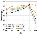
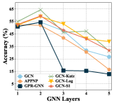
Figure 3: (Left.) Hyper-parameter study with the blend factor $\beta_{0}$ on Cora from 0.01 to 0.99 when $\text{MR}=0.60$. (Right.) Long-range study with the GNN layers from 1 to 5 on Cora when $\text{MR}=0.90$.

5.4 Hyper-parameter Study (RQ3)

In this section, we concentrate on evaluating the influence of different hyper-parameters on GPFN for RQ3. Specifically, we perform a series analysis of blend factor $\beta_{0}$ from the list $[0.01,0.1,0.3,0.5,0.8,0.99]$ to design our infinite graph filter. The left part of Figure 3 depicts the best performance for different filters is respectively achieved when $\beta_{0}=0.5$ and $\beta_{0}=0.8$, emphasizing the significance of scaling blend factor for learning the sparse graph. We notice performance for Katz and S1 drop rapidly when $\beta_{0}=0.99$, while filter Log still performs well. We analyze that Katz and S1 use $\beta_{0}^{n}$ as $\gamma_{n}$ while Log adapts $\gamma_{n}=\frac{\beta_{0}^{n}}{n}$. When $\beta_{0}$ is close to $1$, the weights of every hop in the aggregation matrix are nearly identical from the spatial view, and it can also be analyzed in the spectral domain because the filter function $F_{\gamma}(\cdot)$ allows more high-frequency signals.

5.5 Long-Range Study (RQ4)

In this section, to verify the effectiveness of learning long-range dependencies of GPFN, we vary the GNN layers number from 1 to 5 when $\text{MR}=0.60$ of GCN, APPNP, GPR-GNN, and GCN-Katz on Cora. Theoretically, the spatial receptive field of GNNs expands as layers increase, but the over-smoothing problem that arises in deeper networks makes training harder. As shown in Figure 3, the best performance of all methods is achieved with the small layer due to the over-smoothing. However, our filters exhibit a slower rate of decline, which effectively counteracts the over-smoothing effect than other models. Moreover, our GPFN achieves superior performance with shallow layers compared to others, corresponding to our contribution.

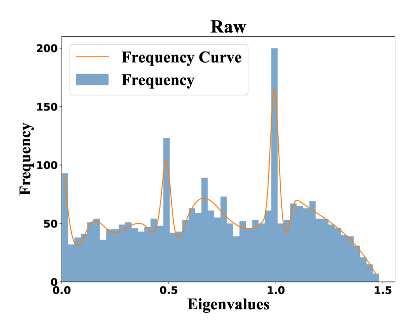
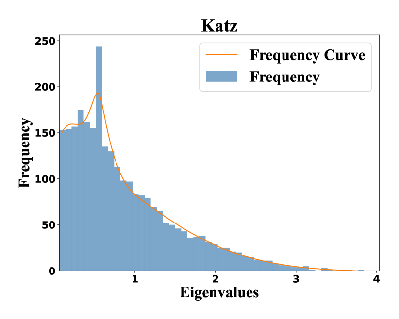
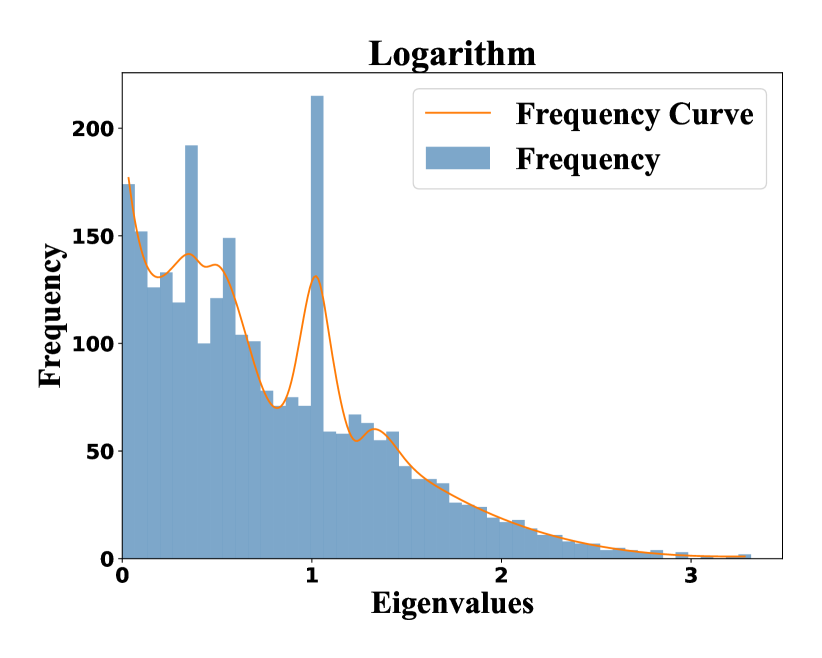
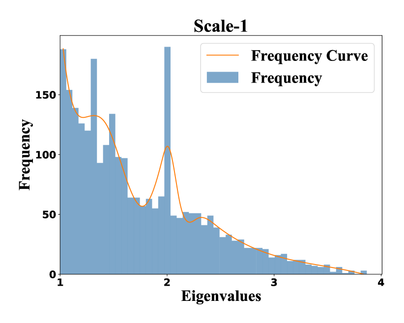
Figure 4: A filter study of Raw (Laplacian Aggregator), Katz, Logarithm and Scale-1 graph filters with $\beta_{0}=0.8$ on Cora. Where $x$-axis is the eigenvalues and $y$-axis is the node frequency.

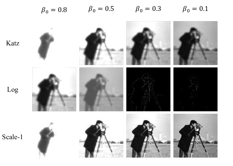
Figure 5: An input image and filtering results with Logarithm, Katz, and Scale-1 graph filters. We also vary $\beta_{0}$ from 0.8 to 0.1.

5.6 Case Study (RQ5)

To answer RQ5, we conduct two case studies on a nature graph and an image to validate the capability of GPFN of Katz, Logarithm, and Scale-1 graph filters.

i) We tested these three filters on Cora and counted their eigenvalues and frequency of $\hat{A}$ in Figure 4. We found that there are still many nodes in the high-frequency signal range $[1.0,1.99]$ (frequency 1.99 was too low to display) of Raw, but after filtering, whether it is Katz, Logarithm, or Scale-1, the distribution of eigenvalues shows a long tail distribution. The frequency of high eigenvalue nodes (corresponding to high-frequency signals) is significantly reduced, indicating that the high-frequency signals have been filtered out. Moreover, it is worth noting that different filters have different ranges of eigenvalues after filtering. For example, when Katz is low-pass, its eigenvalue range is [0, 1/($\lambda_{max}\beta_{0})]$, so Katz’s eigenvalues’ range is from 0 to $1/(1-(1.99-1)\beta_{0})\approx 5$ when $\beta_{0}=0.8$. In addition, compared to Logarithm and Scale-1, Katz’s eigenvalue distribution curve is smoother when $\beta_{0}=0.8$, which proves that Katz’s effect is more effective at this blend factor.

ii) Specifically, given an image with grey values from $0$ to $255$, we first construct a graph in which nodes and edges are the pixels and the links between the nearest 8 neighboring pixels respectively. Then we apply these three filters to the image-based graph. Finally, we reconstruct the image through the filtered graph structure and Figure 5 depicts filtered images with different $\beta_{0}$. According to the visualization, we can derive the following observations: First, we observe that for different graph filters under different $\beta_{0}$, the type and degree are various too. To name some, for Katz and Scale-1, their low-pass effect intensifies with the increase in $\beta_{0}$. However, as for Logarithm, it is a high-pass filter when $\beta_{0}\in(0,0.5)$ while it becomes a low-pass filter when $\beta_{0}\in(0.5,1)$, which verifies our discussion in Section 4.3. Furthermore, when comparing Scale-1 to Katz, we find that the filter effect of Scale-1 experiences a rapid decline as $\beta_{0}$ decreases. This decline can be attributed to Scale-1 imposing a more substantial penalty on distant neighbors with small values of $\beta_{0}$.

6 Conclusion

This paper focuses on the design of power series-enhanced GNNs to address the challenges of long-range dependencies and the sparse graph. To ensure the efficiency of our GPFN, a graph filter using convergent power series from the spectral domain is introduced in this paper. The effectiveness of our GPFN is verified by theoretical analysis from both spectral and spatial perspectives and experimental results, demonstrating its superiority over state-of-the-art graph learning techniques on benchmark datasets. Future directions for investigation include exploring diverse filters such as the mid-pass filter and integrating the diffusion model to further bring the explanation into our GPFN.

Appendix A Prove for Eigenvalue

In this section, we prove that the maximum of $\widetilde{L}_{sym}$ eigenvalue is $2$ iff the graph is bipartite as bellow:

$$R(\widetilde{L}_{sym},u_{i})=\frac{u_{i}^{T}\widetilde{L}_{sym}u_{i}}{u_{i}^{T}u_{i}}=\frac{u_{i}^{T}(I-\widetilde{D}^{-1/2}\widetilde{A}\widetilde{D}^{-1/2})u_{i}}{u_{i}^{T}u_{i}}$$

$$=\frac{u_{i}^{T}\widetilde{D}^{-1/2}(\widetilde{D}-\widetilde{A})\widetilde{D}^{-1/2}u_{i}}{u_{i}^{T}u_{i}}=\frac{q_{i}^{T}(\widetilde{D}-\widetilde{A})q_{i}}{(\widetilde{D}^{1/2}q_{i})^{T}(\widetilde{D}^{1/2}q_{i})}$$

$$=\frac{1}{2}\frac{\sum_{i,j=1}^{N}\widetilde{A}_{ij}(q_{i}-q_{j})^{2}}{\sum_{i=1}^{N}q_{i}^{2}\widetilde{D}_{ii}}.$$

Then, we apply Cauchy-Schwartz inequality to this equation, and we have:

$$R(\widetilde{L}_{sym},u_{i})\leq\frac{\sum_{i,j=1}^{N}\widetilde{A}_{ij}(q_{i}^{2}+q_{j}^{2})}{\sum_{i=1}^{N}q_{i}^{2}\widetilde{D}_{ii}}=\frac{2\sum_{i,j=1}^{N}\widetilde{A}_{ij}q_{i}^{2}}{\sum_{i=1}^{N}q_{i}^{2}\widetilde{D}_{ii}}$$ (8)

$$=\frac{2\sum_{i=1}^{N}u_{i}^{2}/\widetilde{D}_{ii}\sum_{j=1}^{N}\widetilde{A}_{ij}}{\sum_{i=1}^{N}(q_{i}\widetilde{D}^{1/2})^{2}}=2\frac{\sum_{i=1}^{N}\frac{u_{i}^{2}}{\widetilde{D}_{ii}}\widetilde{D}_{ii}}{\sum_{i=1}^{N}u_{i}^{2}}$$

$$=2\frac{\sum_{i=1}^{N}u_{i}^{2}}{\sum_{i=1}^{N}u_{i}^{2}}=2.$$

Thus, when the graph $\mathcal{G}$ is bipartite, the equality holds as $\sum_{i,j=1}^{N}\widetilde{A}_{ij}(q_{i}-q_{j})^{2}=\sum_{i,j=1}^{N}\widetilde{A}_{ij}(q_{i}^{2}+q_{j}^{2})$.

Appendix B Prove for Mitigating Over-Smoothing

B.0.1 Compared to Monomial Graph Filter

In this section, we compare our filter with the traditional graph filter GCN. Recall that message-passing framework can be described as $H^{(K+1)}=\sigma(\hat{A}H^{(K)}W^{(K)})$. For better comparison, we omit the activation function $\sigma(\cdot)$ and the learnable weight matrix $W^{(K)}$ Wu et al. [2019], we have $H^{(K)}=\hat{A}^{(K)}X$. As for. GCN we have $H^{(K)}=\hat{A}^{(K)}X=U^{T}(\Lambda)^{K}UX$. Here we taking Scale-1 for example, we have $H^{(K)}=\hat{A}^{(K)}X=U^{T}F_{\gamma}(\Lambda)^{K}UX$.

After applying $K$ ($K$ is large enough) GNN layers, the over-smoothing phenomenon occurs. That’s to say, the graph embeddings are gradually approaching consensus. Here we assume that the difference between graph embeddings $H^{(K)}$ approach 0, and the embedding of the entire graph can be represented by a full one-vector multiplied by the embedding bound $\mathcal{B}$: $H^{(K)}=\mathcal{B}+o_{K}(1)$, where $\mathcal{B}$ is a low-rank matrix.

As a consequence, for GCN, we have $H^{(K)}_{:j(\text{GCN})}=\mathbf{1[b_{\text{GCN}}]}+o_{K}(1)$ and for Scale-1 we have $H^{(K)}_{:j({\text{Scale-1}})}=\mathbf{1[b_{\text{Scale-1}}]}+o_{K}(1)$ where $j$ denotes the $j$-th node, $\mathbf{1[b_{\text{Scale-1}}]},\mathbf{1[b_{\text{GCN}}]}$ is the boundary when $K\to+\infty$ for Scale-1 and GCN respectively. Next, we compare the convergence rates when different graph filters tend to approach bound with the Euclidean norm:

$$\begin{split}&\lim_{K\to+\infty}\frac{H^{(K)}_{:j({\text{Scale-1}})}-\mathbf{1[b_{\text{Scale-1}}]}}{{H^{(K)}_{:j(\text{GCN})}-\mathbf{1[b_{\text{GCN}}]}}}\\ &=\lim_{K\to+\infty}\frac{f^{(K)}_{\gamma}(\hat{A}_{:j(\text{{Scale-1}})})X-\mathbf{1[b_{\text{{Scale-1}}}}]}{{\hat{A}^{(K)}_{:j(\text{GCN})}X-\mathbf{1[b_{\text{GCN}}]}}}\\ &=\sum_{i=1}^{N}{\lim_{K\to+\infty}}\|{\frac{f^{(K)}_{\gamma}(\lambda_{i(\text{{Scale-1}})})[u_{i}^{T}u_{i}x_{i}]-b_{i({\text{Scale-1}})}}{\lambda^{K}_{i({\text{GCN}})}[u_{i}^{T}u_{i}x_{i}]-b_{i({\text{GCN}})}}}\|_{2}\\ &=\sqrt{\sum_{i=1}^{N}{\lim_{K\to+\infty}}{\frac{f^{(K)}_{\gamma}(\lambda_{i({\text{Scale-1}})})[u_{i}^{T}u_{i}x_{i}]-b_{i({\text{Scale-1}})}}{\lambda^{K}_{i(\text{GCN})}[u_{i}^{T}u_{i}x_{i}]-b_{i(\text{GCN})}}}}.\end{split}$$ (9)

Since both the numerator and the denominator tend to $0$ as $K\to+\infty$, and $m_{i}$ is a variable independent of $K$, we use L’Hôpital’s rule:

$$\begin{split}&\lim_{K\to+\infty}\frac{H^{(K)}_{:j(\text{Scale-1})}-\mathbf{1[m_{\text{Scale-1}}]}}{{H^{(K)}_{:j(\text{GCN})}-\mathbf{1[m_{\text{GCN}}]}}}\\ &=\sqrt{\sum_{i=1}^{N}{\lim_{K\to+\infty}}{\frac{f^{(K)}_{\gamma}(\lambda_{i(\text{Scale-1})})\ln(f_{\gamma}(\lambda_{i(\text{Scale-1})}))[u_{i}^{T}u_{i}x_{i}]}{\lambda^{K}_{i(\text{GCN})}\ln(\lambda_{i(\text{GCN})})[u_{i}^{T}u_{i}x_{i}]}}}\end{split}$$ (10)

As we stated before, $f_{\gamma}(\lambda_{i(\text{Scale-1})})\geq 0$ and has a upper boundary $\mathbf{M}\in\mathbb{R^{+}}$ because $f_{\gamma}(\lambda)$ is convergence. Therefore, the value of this limit primarily depends on the limit of the fraction $\frac{f^{(K)}_{\gamma}(\lambda_{i(\text{Scale-1})})}{\lambda^{K}_{i(\text{GCN})}}$:

$$\begin{split}&\lim_{K\to+\infty}\frac{f^{(K)}_{\gamma}(\lambda_{i(\text{Scale-1})})}{\lambda^{K}_{i(\text{GCN})}}\\ &=\lim_{K\to+\infty}(\frac{1}{\lambda_{i(\text{GCN})}(1-\beta_{0}\lambda_{i(\text{Scale-1})})})^{K}\end{split}$$ (11)

As the eigenvalue of aggregation matrix $\lambda_{i}\in[0,1]$, it’s obviously $\lim_{K\to+\infty}\frac{f^{(K)}_{\gamma}(\lambda_{i({Scale-1})})}{\lambda^{K}_{i({GCN})}}\to+\infty$. Hence we have $o_{K}(1)=H^{(K)}_{({Scale-1})}-\mathbf{1}\mathcal{B}$ is indeed a low order infinitesimal to graph filter as GCN.

Therefore, compared with GCN, GPFN is a lower order infinitesimal of GCN, and its convergence speed is slower when over-smoothing occurs, which also proves that GPFN can alleviate overfitting.

B.0.2 Compared to Polynomial Graph Filter

Following GPR-GNN, we shrink GPFN to Polynomial Graph Filter by replacing $+\infty$ to $K$ and denote it as GPFN-. Therefore, our aim is to explore whether the part of $k\to+\infty$ will play a role in the mitigation of over-smoothing.

As a consequence, for GPFN-, we have $H^{(K)}_{:j({\text{GPFN-}})}=\mathbf{1[b_{\text{GPFN-}}]}+o_{K}(1)$ where $j$ denotes the $j$-th node, $\mathbf{1[b_{\text{GPFN-}}]}$ is the boundary when $K\to+\infty$ for GPFN-. Same as before, we use Scale-1 for comparison and denote GPFN- as Scale-1-. Next, we compare the convergence rates when different graph filters tend to approach bound with the Euclidean norm.

Since both the numerator and the denominator tend to $0$ as $K\to+\infty$, and $m_{i}$ is a variable independent of $K$, we use L’Hôpital’s rule:

$$\begin{split}&\lim_{K\to+\infty}\frac{H^{(K)}_{:j(\text{Scale-1-})}-\mathbf{1[m_{\text{Scale-1-}}]}}{H^{(K)}_{:j(\text{Scale-1})}-\mathbf{1[m_{\text{Scale-1}}]}}\\ &=\sqrt{\sum_{i=1}^{N}{\lim_{K\to+\infty}}{\frac{f^{(K)}_{\gamma}(\lambda_{i(\text{Scale-1-})})\ln(f_{\gamma}(\lambda_{i(\text{Scale-1-})}))[u_{i}^{T}u_{i}x_{i}]}{f^{(K)}_{\gamma}(\lambda_{i(\text{Scale-1})})\ln(f_{\gamma}(\lambda_{i(\text{Scale-1})}))[u_{i}^{T}u_{i}x_{i}]}}}\\ &=\sqrt{\sum_{i=1}^{N}{\lim_{K\to+\infty}}\Bigl{(}1-(\frac{\sum_{n=K}^{+\infty}\gamma_{n}\hat{A}^{n}X}{\sum_{n=0}^{+\infty}\gamma_{n}\hat{A}^{n}X})^{K}\Bigl{)}}.\end{split}$$ (12)

Since $\frac{\sum_{n=K}^{+\infty}\gamma_{n}\hat{A}^{n}X}{\sum_{n=0}^{+\infty}\gamma_{n}\hat{A}^{n}X}>0$, this equation will approach 0. As a consequence:

$$\begin{split}&\lim_{K\to+\infty}\frac{f^{(K)}_{\gamma}(\lambda_{i(\text{Scale-1-})})}{f^{(K)}_{\gamma}(\lambda_{i(\text{Scale-1})})}\\ &=\sqrt{\sum_{i=1}^{N}{\lim_{K\to+\infty}}\Bigl{(}1-(\frac{\sum_{n=K}^{+\infty}\gamma_{n}\hat{A}^{n}X}{\sum_{n=0}^{+\infty}\gamma_{n}\hat{A}^{n}X})^{K}\Bigl{)}}\\ &=0.\end{split}$$ (13)

Hence GPFN- is indeed a high order infinitesimal to graph filter as GPFN.

Therefore, compared with the polynomial graph filter, GPFN is a lower order infinitesimal of GPFN-, and its convergence speed is slower when over-smoothing occurs, which also proves that GPFN can alleviate overfitting.

Appendix C Baselines

Table 4: Baseline Code URLs of Github Repository

Repo	URL
LP	https://github.com/sahipchic/VK-LabelPropogation
GCN	https://github.com/tkipf/gcn
GAT	https://github.com/PetarV-/GAT
GIN	https://github.com/weihua916/powerful-gnns
AGE	https://github.com/thunlp/AGE
SGC	https://github.com/Tiiiger/SGC
ChebGCN	https://github.com/mdeff/cnn_graph
GRP-GNN	https://github.com/jianhao2016/GPRGNN
APPNP	https://github.com/benedekrozemberczki/APPNP
BernNet	https://github.com/ivam-he/BernNet
GRAND	https://github.com/THUDM/GRAND
D2PT	https://github.com/yixinliu233/D2PT
HiGNN	https://github.com/Yiminghh/HiGCN
GPFN	https://github.com/GPFN-Anonymous/GPFN

• MLP Rosenblatt [1963]: MLP simply utilizes the multi-layer perception to perform node classification.

• LP Zhu and Ghahramani [2002]: The method predicts the node class by propagating the known labels in the graph, which does not involve processing node attributes.

• GCN Kipf and Welling [2016]: GCN is a scalable approach for semi-supervised learning on graph-structured data.

• GAT Veličković et al. [2018]: GAT is a spatial domain method, which aggregates information through the attention-learned edge weights.

• GIN Xu et al. [2019]: GIN utilizes a multi-layer perceptron to sum the results of GNN and learns a parameter to control residual connection.

• AGE Cui et al. [2020]: AGE applies a designed Laplacian smoothing filter to better alleviate the high-frequency noises in the node attributes.

• SGC Wu et al. [2019]: SGC is a fixed low-pass filter followed by a linear classifier that reduces the excess complexity by removing nonlinearities and weight matrices between consecutive layers. We combine GCN and GAT with SGC to derive GCN-SGC and GAT-SGC for comparison.

• ChebGCN Defferrard et al. [2016]: ChebGCN is a graph convolutional network that leverages Chebyshev polynomials for efficient graph filtering and representation learning.

• GPR-GNN Eli Chien and Milenkovic [2021]: GPR-GNN learns the weights of representations after information propagation with different steps and performs weighted sum on representations.

• APPNP Gasteiger et al. [2022]: APPNP approximates topic-sensitive PageRank via a random walk to perform information propagation.

• Res Li et al. [2019]: Res avoids excessive smoothness through residual connection. Like SGC Wu et al. [2019], we also remove nonlinear functions and learnable weight to simplify the Res framework. Besides, we also incorporate GCN and GAT into the Res framework as Res-GCN and Res-GAT for comparison.

• BernNet He et al. [2021]: BernNet uses K-order Bernstein polynomials to approximate graph spectral filters and then performs information aggregation by designing polynomial coefficients.

• GRAND Feng et al. [2022]: A generalized forward push (GFPush) algorithm in GRAND+ to pre-compute a general propagation matrix to perform GNN.

• D²PT Liu et al. [2023]: D²PT performs the dual-channel diffusion message passing with the contrastive-enhanced global graph information on the sparse graph.

• HiGNN Huang et al. [2023]: HiGNN proposes a higher-order graph convolutional network grounded in Flower-Petals Laplacians to discern complex features across different topological scales.

• HiD-GCN Li et al. [2024]: A high-order neighbor-aware graph diffusion network.

Appendix D Hyper-parameter Settings of Baselines

For GPR-GNN, HiGNN and HiD-GCN, we use the officially released code and other baseline models are based on Pytorch Geometric implementation  Fey and Lenssen [2019]. Table  4 shows the code we used.

The parameters of baselines are also optimized using the Adam with $L_{2}$ regularization. We set the learning rate at 0.002 with a weight decay of 0.005. Besides, we employ the early-stopping strategy with patience equal to 20 to avoid over-fitting.

For MLP, we use 2 layers of a fully connected network with 32 hidden units. For GCN, we use 2 GCN layers with 16 hidden units. For GAT, the first layer has 8 attention heads and each head has 8 hidden units, and the second layer has 1 attention head and 16 hidden units. For GIN, we use two layers with 16 hidden units. For ChebGCN, we use 2 propagation steps with 32 hidden units in each layer. For APPNP, we use a 2-layer MLP with 64 hidden units and set the propagation step K to 10. For GPR-GNN, we use a 2-layer MLP with 64 hidden units and set the propagation steps K to 10, and use PPR initialization. For BernNet, we use a 2-layer MLP with 64 hidden units and set the propagation step K to 10. For SGC, we set layers at K=3.

References

- Ahad N. et al. [2023] Zehmakan Ahad N., Out Charlotte, and Khelejan Sajjad Hesamipour. Why rumors spread fast in social networks, and how to stop it. In IJCAI, 2023.
- Berger et al. [2005] Noam Berger, Christian Borgs, Jennifer T. Chayes, and Amin Saberi. On the spread of viruses on the internet. In SODA, 2005.
- Chatterjee and Huang [2024] Anirban Chatterjee and Jiaoyang Huang. Fluctuation of the largest eigenvalue of a kernel matrix with application in graphon-based random graphs, 2024.
- Cui et al. [2020] Ganqu Cui, Jie Zhou, Cheng Yang, and Zhiyuan Liu. Adaptive graph encoder for attributed graph embedding. In SIGKDD, 2020.
- Defferrard et al. [2016] Michaël Defferrard, Xavier Bresson, and Pierre Vandergheynst. Convolutional neural networks on graphs with fast localized spectral filtering. In NeurIPS, 2016.
- Eli Chien and Milenkovic [2021] Pan Li Eli Chien, Jianhao Peng and Olgica Milenkovic. Adaptive universal generalized pagerank graph neural network. In ICLR, 2021.
- Fang et al. [2023] Yuchen Fang, Yanjun Qin, Haiyong Luo, Fang Zhao, Bingbing Xu, Liang Zeng, and Chenxing Wang. When spatio-temporal meet wavelets: Disentangled traffic forecasting via efficient spectral graph attention networks. In ICDE, 2023.
- Feng et al. [2022] Wenzheng Feng, Yuxiao Dong, Tinglin Huang, Ziqi Yin, Xu Cheng, Evgeny Kharlamov, and Jie Tang. Grand+: Scalable graph random neural networks. In WWW, 2022.
- Fey and Lenssen [2019] Matthias Fey and Jan Eric Lenssen. Fast graph representation learning with pytorch geometric, 2019.
- Gao et al. [2023] Xiaowei Gao, Huanfa Chen, and James Haworth. A spatiotemporal analysis of the impact of lockdown and coronavirus on london’s bicycle hire scheme: from response to recovery to a new normal. GIS, 2023.
- Gasteiger et al. [2022] Johannes Gasteiger, Aleksandar Bojchevski, and Stephan Günnemann. Predict then propagate: Graph neural networks meet personalized pagerank. In ICLR, 2022.
- Guo et al. [2024] Jingwei Guo, Kaizhu Huang, Xinping Yi, Zixian Su, and Rui Zhang. Rethinking spectral graph neural networks with spatially adaptive filtering, 2024.
- Hamilton et al. [2017] Will Hamilton, Zhitao Ying, and Jure Leskovec. Inductive representation learning on large graphs. In NeurIPS, 2017.
- He et al. [2021] Mingguo He, Zhewei Wei, zengfeng Huang, and Hongteng Xu. Bernnet: Learning arbitrary graph spectral filters via bernstein approximation. In NeurIPS, 2021.
- Huang et al. [2023] Yiming Huang, Yujie Zeng, Qiang Wu, and Linyuan Lü. Higher-order graph convolutional network with flower-petals laplacians on simplicial complexes, 2023.
- Jiang et al. [2023] Xinke Jiang, Dingyi Zhuang, Xianghui Zhang, Hao Chen, Jiayuan Luo, and Xiaowei Gao. Uncertainty quantification via spatial-temporal tweedie model for zero-inflated and long-tail travel demand prediction. In CIKM, 2023.
- Jiang et al. [2024] Xinke Jiang, Zidi Qin, Jiarong Xu, and Xiang Ao. Incomplete graph learning via attribute-structure decoupled variational auto-encoder. In WSDM, 2024.
- Jin et al. [2022] Wei Jin, Xiaorui Liu, Yao Ma, Charu Aggarwal, and Jiliang Tang. Feature overcorrelation in deep graph neural networks: A new perspective. In SIGKDD, 2022.
- Kingma and Ba [2015] Diederik P. Kingma and Jimmy Ba. Adam: A method for stochastic optimization. In ICLR, 2015.
- Kipf and Welling [2016] Thomas N. Kipf and Max Welling. Semi-supervised classification with graph convolutional networks. In ICLR, 2016.
- Li et al. [2019] Guohao Li, Matthias Müller, Ali Thabet, and Bernard Ghanem. Deepgcns: Can gcns go as deep as cnns? In ICCV, 2019.
- Li et al. [2022] Rongfan Li, Ting Zhong, Xinke Jiang, Goce Trajcevski, Jin Wu, and Fan Zhou. Mining spatio-temporal relations via self-paced graph contrastive learning. In SIGKDD, 2022.
- Li et al. [2024] Yibo Li, Xiao Wang, Hongrui Liu, and Chuan Shi. A generalized neural diffusion framework on graphs. In AAAI, 2024.
- Liu et al. [2023] Yixin Liu, Kaize Ding, Jianling Wang, Vincent Lee, Huan Liu, and Shirui Pan. Learning strong graph neural networks with weak information. In SIGKDD, 2023.
- Luxburg [2007] Ulrike Luxburg. A tutorial on spectral clustering, 2007.
- Matsugu et al. [2023] Shohei Matsugu, Yasuhiro Fujiwara, and Hiroaki Shiokawa. Uncovering the largest community in social networks at scale. In IJCAI, 2023.
- Monti et al. [2016] Federico Monti, Davide Boscaini, Jonathan Masci, Emanuele Rodolà, Jan Svoboda, and Michael M. Bronstein. Geometric deep learning on graphs and manifolds using mixture model cnns. In NeurIPS, 2016.
- Nica [2018] Bogdan Nica. A Brief Introduction to Spectral Graph Theory. EMS Press, 2018.
- Ortega et al. [2018] Antonio Ortega, Pascal Frossard, Jelena Kovačević, José M. F. Moura, and Pierre Vandergheynst. Graph signal processing: Overview, challenges, and applications. IEEE, 2018.
- Paszke et al. [2019] Adam Paszke, Sam Gross, Francisco Massa, Adam Lerer, James Bradbury, Gregory Chanan, Trevor Killeen, Zeming Lin, Natalia Gimelshein, Luca Antiga, Alban Desmaison, Andreas Kopf, Edward Yang, Zachary DeVito, Martin Raison, Alykhan Tejani, Sasank Chilamkurthy, Benoit Steiner, Lu Fang, Junjie Bai, and Soumith Chintala. Pytorch: An imperative style, high-performance deep learning library. In NeurIPS, 2019.
- Qin et al. [2022] Yanjun Qin, Yuchen Fang, Haiyong Luo, Fang Zhao, and Chenxing Wang. Next point-of-interest recommendation with auto-correlation enhanced multi-modal transformer network. In SIGIR, 2022.
- Rosenblatt [1963] Frank Rosenblatt. Principles of neurodynamics. perceptrons and the theory of brain mechanisms. AJP, 1963.
- Rusch et al. [2023] T. Konstantin Rusch, Michael M. Bronstein, and Siddhartha Mishra. A survey on oversmoothing in graph neural networks, 2023.
- Shuman et al. [2013] D. I. Shuman, S. K. Narang, P. Frossard, A. Ortega, and P. Vandergheynst. The emerging field of signal processing on graphs: Extending high-dimensional data analysis to networks and other irregular domains. IEEE Signal Processing Magazine, 2013.
- Veličković et al. [2018] Petar Veličković, Guillem Cucurull, Arantxa Casanova, Adriana Romero, Pietro Liò, and Yoshua Bengio. Graph attention networks. In ICLR, 2018.
- Wolpert and Macready [1997] D.H. Wolpert and W.G. Macready. No free lunch theorems for optimization. IEEE Transactions on Evolutionary Computation, 1997.
- Wu et al. [2019] Felix Wu, Amauri Holanda de Souza, Tianyi Zhang, Christopher Fifty, Tao Yu, and Kilian Q. Weinberger. Simplifying graph convolutional networks. In ICML, 2019.
- Xu et al. [2019] Keyulu Xu, Weihua Hu, Jure Leskovec, and Stefanie Jegelka. How powerful are graph neural networks? In ICLR, 2019.
- Zhu and Ghahramani [2002] Xiaojin Zhu and Zoubin Ghahramani. Learning from labeled and unlabeled data with label propagation. Citeseer, 2002.