Discretization of fractional fully nonlinear equations by powers of discrete Laplacians

Abstract.

We study discretizations of fractional fully nonlinear equations by powers of discrete Laplacians. Our problems are parabolic and of order $\sigma\in(0,2)$ since they involve fractional Laplace operators $(-\Delta)^{\sigma/2}$. They arise e.g. in control and game theory as dynamic programming equations, and solutions are non-smooth in general and should be interpreted as viscosity solutions. Our approximations are realized as finite-difference quadrature approximations and are 2nd order accurate for all values of $\sigma$. The accuracy of previous approximations depend on $\sigma$ and are worse when $\sigma$ is close to $2$. We show that the schemes are monotone, consistent, $L^{\infty}$-stable, and convergent using a priori estimates, viscosity solutions theory, and the method of half-relaxed limits. We present several numerical examples.

1. Introduction

In this paper we introduce and analyze numerical schemes based on powers of the discrete Laplacian in the context of nonlocal fully nonlinear equations. Our equations involve fractional Laplacians, pseudo-differential operators that can be defined equivalently as Fourier multipliers, singular integral operators, or powers of the Laplacian [1, 38]: For $\sigma\in(0,2)$,

$$-(-\Delta)^{\frac{\sigma}{2}}\phi(x) =\mathcal{F}^{-1}\big{[}-|\xi|^{\sigma}\hat{\phi}(\xi)\big{]}(x)$$

$$=\lim_{r\to 0}\int_{|z|>r}\Big{(}\phi(x+z)-\phi(x)\Big{)}\,\frac{c}{|z|^{N+\sigma}}dz$$

(1.1) $$=\frac{1}{|\Gamma(-\frac{\sigma}{2})|}\,\int_{0}^{\infty}\Big{(}e^{t\Delta}\phi(x)-\phi(x)\Big{)}\,\frac{dt}{t^{1+\frac{\sigma}{2}}}.$$

We discretize this operator by powers of the discrete Laplacian,

(1.2) $$\Delta_{h}\phi(x)=\sum_{k=1}^{N}\frac{\phi(x+he_{k})-2\phi(x)+\phi(x-he_{k})}{h^{2}},$$

denoted by $-(-\Delta_{h})^{\frac{\sigma}{2}}$ and obtained from (1.1) by replacing $\Delta$ by $\Delta_{h}$ [20], cf. (3.1).

The equations we consider are fully-nonlinear, possibly (strongly) degenerate equations from optimal control and differential game theory, equations with a large number of applications in engineering, science, economics, etc. [6, 30, 42, 32]:

(1.3) $$u_{t}-F(x,t,Du,-(-\Delta)^{\frac{\sigma}{2}}u)=0\mbox{\quad in}\quad\mathbb{R}^{N}\times(0,T]=:Q_{T},$$

or more generally, Hamilton-Jacobi-Bellmann(HJB)/Isaacs equations

(1.4) $$u_{t}-\inf_{\beta\in\mathcal{B}}\sup_{\alpha\in\mathcal{A}}\left\{\mathcal{L}^{\alpha,\beta}u-c^{\alpha,\beta}(x,t)u+f^{\alpha,\beta}(x,t)\right\}=0\mbox{\quad in}\quad Q_{T},$$

where $\mathcal{A}$, $\mathcal{B}$ are compact sets and $\mathcal{L}^{\alpha,\beta}$ is the $\sigma\wedge 1$ order drift-diffusion operator

$$\mathcal{L}^{\alpha,\beta}\phi(x):=-a^{\alpha,\beta}(x,t)(-\Delta)^{\frac{\sigma}{2}}\phi(x)+b^{\alpha,\beta}(x,t)\cdot D\phi(x).$$

Equation (1.4) is the dynamic programming equation for a finite horizon optimal stochastic differential game [7, 42, 32], see Section 2.2 for the details.

Equation (1.3) can be degenerate parabolic as we allow $F$ to be non-decreasing in last variable. The solutions are not smooth in general. Even for nonconvex uniformly parabolic problems, the solutions could be too irregular for the equation to hold pointwise. The correct notion of (weak) solution for this type of problems is viscosity solutions [34, 35, 4]. Wellposedness, regularity, and other properties of viscosity solutions for nonlocal fully nonlinear PDEs has been intensely studied in recent years. Regularity in the degenerate case comes from comparison type of arguments and typically gives preservation of the regularity of the data [35]. Solutions are therefore often no more than Lipschitz continuous, see Section 4.1 for an example.

There is an extensive literature on numerical methods for local fully nonlinear equations including finite differences, semi-Lagrangian, finite elements, spectral, Monte Carlo, and many more, see e.g. [24, 46, 37, 29, 5, 15, 39, 14, 12, 26, 45, 13, 31]. Here there is the added difficulty of discretizing the fractional and nonlocal operators in a monotone, stable, and consistent way. These operators are singular integral operators, and can be discretized by quadrature after truncating the singular part and correcting with a suitable second derivative term [23]. In the setting of nonlocal Bellman-Isaacs equations, such approximations were introduced in [36, 16, 10] with further developments, including error estimates, in e.g. [8, 21, 43, 27, 9, 10, 36]. These approximations has fractional order accuracy, depending on the order of the fractional/nonlocal operator.

The numerical approximations used in this paper are based on powers of discrete Laplacians. As opposed to the approximations above, they are 2nd order accurate regardless of the order of the operators. They can also interpreted as quadrature rules and represented as a infinite series expansion with explicit weights [19]. These weights satisfy a discrete version of the Lévy integrability condition. Previously powers of discrete Laplacians have been used to discretize linear equations [25], porous medium equations [28], and very recently also certain HJB equations [18]. In [18], (optimal fractional) error bounds for numerical schemes for convex fractional equations are studied. But in the case of powers of the discrete Laplacian, only very simple non-degenerate constant coefficient problems were considered, and no numerical experiments were performed. This paper gives extensions of the schemes and convergence results in [18] to a very large class of fully nonlinear equations, including non-convex, strongly degenerate, and variable coefficients problems. We show that the resulting schemes are consistent, monotone, stable, and convergent. We do not study error bounds, but we perform a number of numerical experiments.

To simplify the presentation we introduce the numerical scheme and perform the detailed convergence analysis for the following version of the problem:

(1.5) $$u_{t}-F\big{(}-(-\Delta)^{\frac{\sigma}{2}}u\big{)} =f(x,t),\hskip 14.22636pt (x,t) \in Q_{T},$$

$$u(x,0) =u_{0}(x), x \in\mathbb{R}^{N},$$

We also focus on explicit schemes using forward Euler time discretizations. Under suitable CFL conditions, we then show that the schemes are monotone satisfying a comparison principle and $L^{\infty}$-stable. We use viscosity solutions and the Barles-Perthame-Souganidis method of half-relaxed limits [5] to show that solutions of the schemes converge uniformly to solutions of the equation. To do that, we show that the particular versions of monotonicity and consistency required by [5] are indeed satified by our schemes. Numerical examples are presented for problem (1.5), in one and two dimension, for problems with non-smooth and smooth solutions. We also illustrate numerically the convergence of solutions as $\sigma\to 0^{+}$ and $\sigma\to 2^{-}$, showing that our schemes are stable also with respect to these limits. Later (Section 5) we explain how to extend the schemes and results to other time-discretisations and more general problems, including problems with first order/convection terms, and the Bellman-Isaacs equation (1.3).

The remaining part of this paper is organized as follows: In Section 2 we introduce the notation and assumptions, and give well-posedness results for equation (1.5). In addition, we discuss the relation between HJB-Isaacs equations and a zero sum game. In Section 3 we give the results for approximations based on powers of discrete Laplacians and show the convergence of the schemes. Numerical examples are presented in Section 4, and Section 5 covers extensions of the results for various cases, e.g. other time discretization, equation involving convection, HJB-Isaacs type equations.

2. On nonlocal PDEs

In this section we present the assumptions on the nonlocal fully nonlinear equation (1.5) and give wellposedness and regularity results. In the second part we explain the connection between the HJB/Isaacs equation (1.4) and a stochastic differential game.

Let us first introduce some notation. By $C,K$ etc. we mean various constants which may change from line to line, $|\cdot|$ is the euclidean norm, and the norms $\|u\|_{L^{\infty}}=\sup_{x}|u(x)|$ and $\|u\|_{W^{1,\infty}}=\|u\|_{L^{\infty}}+\sup_{x\neq y}\frac{|u(x)-u(y)|}{|x-y|}$. $C_{b}(Q)$ is the space of bounded continuous functions on $Q\subset\mathbb{R}^{N}$, while $C^{n}(Q)$ for $n\in\mathbb{N}$ denote the spaces of $n$-th time continuously differentiable functions on $Q$ with finite norms $\|u\|_{n}=\sum_{j=0}^{n}\|D^{j}u\|_{L^{\infty}}$. By $\text{USC}_{b}(Q)$ and $\text{LSC}_{b}(Q)$, we denote the space of bounded upper and lower semicontinuous function on $Q$.

2.1. Wellposedness of nonlocal PDEs

We will study viscosity solutions of equation (1.5) under the following assumptions:

1. $F(l_{1})-F(l_{2})\leq L_{F}(l_{1}-l_{2})^{+}$ for all $l_{1},l_{2}\in\mathbb{R}$.

2. $f\in C_{b}(Q_{T})$ and $u_{0}\in C_{b}(\mathbb{R}^{d})$.

Assumption $\mathbf{(A1)}$ implies that $F$ is both Lipschitz continous (with Lipschitz constant $L_{F}$) and nondecreasing. A definition and general theory of viscosity solution for the nonlocal equations like (1.4) can be found e.g. in [34, 4], but we do not need this generality here. In particular since there is no local diffusion, we could follow the simpler (comparison) arguments of [17].

We have the following strong comparison and well-posedness results for (1.5):

Proposition 2.1.

Assume $\mathbf{(A1)}$ and $\mathbf{(A2)}$.

(i) (Comparison) If $u\in\text{USC}_{b}$ and $v\in\text{LSC}_{b}$ are bounded viscosity subsolution and supersolution of (1.5) respectively, then

$$u\leq v\text{ in }\mathbb{R}^{N}\times[0,T].$$

(ii) (Existence and uniqueness) There exists a unique bounded continuous viscosity solution $u$ of (1.5).

(iii) ($L^{\infty}$-stability) The solution $u$ in (ii) satisfies:

$$\|u(\cdot,t)\|_{L^{\infty}}\leq\|u_{0}\|_{L^{\infty}}+t\big{(}\|f\|_{L^{\infty}}+|F(0)|\big{)}.$$

Proof.

We refer [17, Section 6] for part (i) and (ii) in the case when $u_{0}$ and $f$ are $BUC$. As mentioned there, the parabolic proof is a simple generalization of the detailed proofs in the elliptic case in [17, Theorem 2.1, 2.3 and Corollary 2.2]. These proofs easily extend to the case when $u_{0}$ and $f$ are $C_{b}$.
   For (iii), begin by defining

$$w(x,t)=\|u_{0}\|_{L^{\infty}(\mathbb{R}^{N})}+t(|F(0)|+\|f\|_{L^{\infty}(Q_{T})}).$$

Inserting $w$ into the left-hand side of (1.5), we find that it is a supersolution of the equation:

$$w_{t}-F((-\Delta)^{\frac{\sigma}{2}}w) =(|F(0)|+\|f\|_{L^{\infty}})-F(0)\geq f,$$

where we get $F(0)$ in the first equality since $w$ is independent of $x$. Similarly, $-w$ is a subsolution of (1.5). Then the result follows by part (i). ∎

2.2. A differential game related to nonlocal PDEs

The HJB/Isaacs equation (1.4) is related to a zero sum differential game where players control the following SDE [1, 22] driven by a $\sigma$-stable Levy process of the form

(2.1) $$dX_{s}=b^{\alpha_{s},\beta_{s}}(X_{s},s)\,ds+\int_{|z|>0}\eta^{\alpha_{s},\beta_{s}}(X_{s^{-}},s)z\,\tilde{N}(dz,ds),\quad X_{t}=x,$$

when $\eta^{\alpha,\beta}(x,t)=[a^{\alpha,\beta}(x,t)]^{\frac{1}{\sigma}}$ and $\tilde{N}$ is the compensated Poisson random measure.

The Poisson random measure $N(B,t)$ counts the number of jumps $z\in B$ of the driving process up to time $t$ [1, 42]. For $\sigma$-stable processes, $\mathbb{E}\big{[}N(dz,dt)\big{]}=\nu(dz)dt$ with $\nu(dz)=\frac{cdz}{|z|^{N+\sigma}}$ and then the compensated measure $\tilde{N}(dx,dt)=N(dz,dt)-\nu(dz)dt$. Note that by self-similarity of the definition of the fractional Laplacian and the definition of $\eta^{\alpha,\beta}$,

$$-a^{\alpha,\beta}(x,t)(-\Delta)^{\frac{\sigma}{2}}\phi(x)=p.v.\int_{|z|>0}\big{(}\phi(x+\eta^{\alpha,\beta}(x,t)z)-\phi(x)\big{)}\,\frac{c}{|z|^{N+\sigma}}dz,$$

and hence the generator of $X_{s}$ in (2.1) is the operator $\mathcal{L}^{\alpha,\beta}$ in (1.4) [1, 22].

The game setting is a zero-sum game with two players, separate controls $\alpha_{\cdot}$ and $\beta_{\cdot}$ belonging to sets of admissible controls $\mathcal{A}_{\text{ad}}$ and $\mathcal{B}_{\text{ad}}$, and a “cost” function

$$J(x,t,\alpha_{\cdot},\beta_{\cdot}) =E\Big{[}\int_{t}^{T}e^{-\int_{t}^{s}c^{\alpha_{r},\beta_{r}}(X_{r},r)dr}f^{\alpha_{s},\beta_{s}}(X_{s},s)\,ds$$

$$\hskip 113.81102pt+e^{-\int_{t}^{T}c^{\alpha_{r},\beta_{r}}(X_{r},r)dr}u_{0}(X_{T})\Big{]},$$

where $c$, $f$, and $u_{0}$ are the discounting rate, running cost, and terminal cost respectively. The “cost” function is a cost for one player who seeks to minimise it and a gain for the other who seeks to maximise it. The game can be understood from the (upper/lower) values of the game defined as

$$u(x,T-t)=\inf_{\alpha_{\cdot}\in\mathcal{A}_{\text{ad}}}\sup_{\beta_{\cdot}\in\mathcal{B}_{\text{ad}}}J(x,t,\alpha_{\cdot},\beta_{\cdot}).$$

In the dynamic programming approach to optimal control and differential games [7, 42, 32], this function is shown to satisfy the HJB/Isaacs equation (1.4) with initial data $u_{0}$.

3. Discretization by powers of discrete Laplacian

In this section we approximate the nonlocal fully nonlinear HJB/Isaacs equation (1.5) using a forward Euler approximation in time and powers of the discrete Laplacian to approximate the fractional Laplacians. We then show that the resulting scheme is consistent, monotone, and $L^{\infty}$-stable. Using the method of half-relaxed limits of Barles-Perthame-Souganidis [5], we then show convergence of the method toward the viscosity solution of (1.5).

We introduce space and time grids, $\mathcal{G}_{h}=h\mathbb{Z}^{N}=\{x_{\mathbf{j}}=h\mathbf{j}:\mathbf{j}\in\mathbb{Z}^{N}\}$ and $\mathcal{T}_{\tau}^{T}=\{t_{n}:=n\tau\}_{n=0}^{M}$, for $\tau=\frac{T}{M}>0$, $M\in\mathbb{N}$. The parameters $h$ and $\tau$ are then the distance between the grid points in the two grids.

3.1. Powers of the discrete Laplacian

Let $\Delta_{h}\phi(x)$ be the discrete Laplacian, the 2nd order central finite difference approximation of $\Delta\phi$ defined in (1.2). Then the powers of the discrete Laplacian [19, 28] is defined as

(3.1) $$-(-\Delta_{h})^{\frac{\sigma}{2}}\phi(x):=\frac{1}{|\Gamma(-\frac{\sigma}{2})|}\,\int_{0}^{\infty}\Big{(}e^{t\Delta_{h}}\phi(x)-\phi(x)\Big{)}\,\frac{dt}{t^{1+\frac{\sigma}{2}}},\quad\sigma\in(0,2),$$

where $U(t)=e^{t\Delta_{h}}\psi$ is the solution of semi-discrete heat equation

$$\partial_{t}U(x,t) =\Delta_{h}\,U(x,t)\quad\mbox{for}\quad(x,t)\in\mathbb{R}^{N}\times(0,\infty),$$

$$U(x,0) =\psi(x)\quad\mbox{for}\quad x\in\mathbb{R}^{N}.$$

An explicit formula for $e^{t\Delta_{h}}\phi$ and details related to this approximation can be found in Section 4.5 of [28].

The operator $-(-\Delta_{h})^{\frac{\sigma}{2}}$ is a monotone (positive coefficients) operator given by a series expansion with explicit weights, and these weights satisfy a discrete version of the Levy integrability condition.

Lemma 3.1.

Let $-(-\Delta_{h})^{\frac{\sigma}{2}}$ be defined by (3.1). Then

$$-(-\Delta_{h})^{\frac{\sigma}{2}}\phi(x)=\sum_{\mathbf{j}\in\mathbb{Z}^{N}\setminus\{0\}}\Big{(}\phi(x+x_{\mathbf{j}})-\phi(x)\Big{)}\kappa_{h,\mathbf{j}},$$

where

$$\kappa_{h,\mathbf{j}}=\frac{1}{h^{\sigma}}\frac{1}{|\Gamma(-\frac{\sigma}{2})|}\int_{0}^{\infty}G(\mathbf{j},t)\frac{\text{d}t}{t^{1+\frac{\sigma}{2}}},$$

$G(\mathbf{j},t)=e^{-2Nt}\prod_{i=1}^{N}I_{|\mathbf{j}_{i}|}(2t)$, and $I_{m}\geq 0$ is the modified Bessel function of the first kind and order $m\in\mathbb{N}$. Moreover, $\kappa_{h,\mathbf{j}}\geq 0$ for all $\mathbf{j}\in\mathbb{Z}^{N}$ and there is a $C_{\sigma}>0$ such that

$$\sum_{\mathbf{j}\in\mathbb{Z}^{N}\backslash\{0\}}\kappa_{h,\mathbf{j}}=\frac{C_{\sigma}}{h^{\sigma}}.$$

Note that the last part of the lemma (the formula for the sum) seems not to have been proved before, even though something like this is needed in [28].

Proof.

In the one dimensional case, the results follow from [19, Theorem 1.1]. For the proof of the quadrature representation, see [28, Lemma 4.20].

Note that $G\geq 0$ and then also $\kappa_{h,\mathbf{j}}\geq 0$. For the final result we use from [20, Section 8.2.] that $\sum_{\mathbf{j}\in\mathbb{Z}^{N}}G(\mathbf{j},t)=1$ to see that

(3.2) $$\sum_{\mathbf{j}\in\mathbb{Z}^{N}\backslash\{0\}}\kappa_{h,\mathbf{j}} =\frac{1}{h^{\sigma}}\frac{1}{|\Gamma(-\frac{\sigma}{2})|}\sum_{\mathbf{j}\in\mathbb{Z}^{N}\backslash\{0\}}\int_{0}^{\infty}G(\mathbf{j},t)\frac{\text{d}t}{t^{1+\frac{\sigma}{2}}}$$

$$=\frac{1}{h^{\sigma}}\frac{1}{|\Gamma(-\frac{\sigma}{2})|}\int_{0}^{\infty}(1-G(0,t))\frac{\text{d}t}{t^{1+\frac{\sigma}{2}}},$$

where we interchange the sum and integral by Tonelli’s theorem.

We must show that the integral in the above expression converges. To this end, write

$$\int_{0}^{\infty}(1-G(0,t))\frac{\text{d}t}{t^{1+\frac{\sigma}{2}}}=\underbrace{\int_{0}^{1}(1-G(0,t))\frac{\text{d}t}{t^{1+\frac{\sigma}{2}}}}_{:=I_{1}}+\underbrace{\int_{1}^{\infty}(1-G(0,t))\frac{\text{d}t}{t^{1+\frac{\sigma}{2}}}}_{:=I_{2}}.$$

$I_{2}$ clearly converges, since

$$I_{2}\leq\int_{1}^{\infty}\frac{1}{t^{1+\frac{\sigma}{2}}}dt<\infty,$$

for $\sigma\in(0,2)$.

Showing that $I_{1}$ converges requires a bit more work. Using the definitions of $G$ and of modified Bessel functions of the first kind we can write

$$G(0,t)=e^{-2Nt}\Big{(}1+\sum_{m=1}^{\infty}\frac{t^{2m}}{(m!)^{2}}\Big{)}^{N}.$$

The infinite sum in the above expression is a power series with infinite radius of convergence. Consequently, $G(0,t)$ is a smooth function on the whole real line. In particular, $G(0,\cdot)\in C^{1}([0,1])$. By the mean value theorem, we then have that

$$\frac{G(0,t)-1}{t}=G^{\prime}(s)\qquad\text{for some}\qquad s\in(0,t),$$

where we use that $G(0,0)=1$. Let $M=\max_{s\in[0,1]}|G^{\prime}(s)|$ (which exists since $G(0,\cdot)\in C^{1}([0,1])$). Consequently,

$$I_{1}\leq\int_{0}^{1}\frac{M}{t^{\frac{\sigma}{2}}}dt<\infty,$$

for $\sigma\in(0,2)$.

Since $I_{1}$ and $I_{2}$ converges, we have shown that

$$\sum_{\mathbf{j}\in\mathbb{Z}^{N}\backslash\{0\}}\kappa_{h,\mathbf{j}}=C_{\sigma}\frac{1}{h^{\sigma}},$$

for some constant $C_{\sigma}>0$ and $\sigma\in(0,2)$. The constant $C_{\sigma}$ is strictly greater than zero since the integrand in (3.2) is positive almost everywhere on the domain of integration. ∎

By Lemma 4.22 in [28], $-(-\Delta_{h})^{\frac{\sigma}{2}}$ is a second order approximation of $-(-\Delta)^{\frac{\sigma}{2}}$:

Lemma 3.2 ([28]).

Assume $\sigma\in(0,2)$. Then for any smooth bounded function $\phi$,

(3.3) $$\big{|}(-\Delta_{h})^{\frac{\sigma}{2}}\phi(x)-(-\Delta)^{\frac{\sigma}{2}}\phi(x)\big{|}\leq Ch^{2}\big{(}\|D^{4}\phi\|_{L^{\infty}}+\|\phi\|_{L^{\infty}}\big{)}.$$

From Lemma 3.1 and 3.3 it follows that $-(-\Delta_{h})^{\frac{\sigma}{2}}$ is a monotone (positive coefficients) quadrature approximation of $-(-\Delta)^{\frac{\sigma}{2}}$ satisfying a discrete Levy condition.

3.2. Numerical approximation of the nonlocal PDE

Approximating time derivatives by forward Euler and fractional Laplacians by powers of discrete Laplacians (3.1), we get the following explicit scheme:

(3.4) $$\begin{split}U_{\mathbf{i}}^{n+1}&=U_{\mathbf{i}}^{n}+\tau\Big{[}F\big{(}-(-\Delta_{h})^{\frac{\sigma}{2}}U_{\mathbf{i}}^{n}\big{)}+f_{\mathbf{i}}^{n}\Big{]}\qquad\text{for}\qquad\mathbf{i}\in\mathbb{Z}^{N},n\in\mathcal{T}_{\tau}^{T},\\ U_{\mathbf{i}}^{0}&=u_{0}\qquad\text{for}\qquad\mathbf{i}\in\mathbb{Z}^{N},\end{split}$$

where $U_{\mathbf{i}}^{n}=u(x_{\mathbf{i}},t_{n})$ and $f_{\mathbf{i}}^{n}=f(x_{\mathbf{i}},t_{n})$ for $x_{\mathbf{i}}\in\mathcal{G}_{h}$ and $t_{n}\in\mathcal{T}_{\tau}^{T}$.

This scheme is monotone/satisfies a comparison principle under a CFL condition:

(3.5) $$\tau\leq\frac{1}{L_{F}C_{\sigma}}h^{\sigma},\qquad\text{$C_{\sigma}$ and $L_{F}$ are given by Lemma \ref{lem::discr_fraclap_quadrature} and \ref{F1}}.$$

Theorem 3.3 (Comparison).

Assume $\mathbf{(A1)}$, (3.5), and $U,V$ sub-, supersolutions of (3.4). If $U_{\mathbf{j}}^{0}\leq V_{\mathbf{j}}^{0}$ for all $\mathbf{j}\in\mathbb{Z}^{N}$, then $U_{\mathbf{j}}^{n}\leq V_{\mathbf{j}}^{n}$ holds for all $n\geq 1$ and $\mathbf{j}\in\mathbb{Z}^{N}$.

Proof.

Consider the following calculation:

$$U_{\mathbf{i}}^{1}-V_{\mathbf{i}}^{1}$$

$$\leq U_{\mathbf{i}}^{0}-V_{\mathbf{i}}^{0}+\tau\Big{(}F\big{(}-(-\Delta_{h})^{\frac{\sigma}{2}}U_{\mathbf{i}}^{0}\big{)}-F\big{(}-(-\Delta_{h})^{\frac{\sigma}{2}}V_{\mathbf{i}}^{0}\big{)}\Big{)}$$

$$\leq U_{\mathbf{i}}^{0}-V_{\mathbf{i}}^{0}+\tau L_{F}\cdot\Big{(}-(-\Delta_{h})^{\frac{\sigma}{2}}\big{(}U_{\mathbf{i}}^{0}-V_{\mathbf{i}}^{0}\big{)}\Big{)}^{+}$$

$$=U_{\mathbf{i}}^{0}-V_{\mathbf{i}}^{0}+\tau L_{F}\cdot\Big{(}\sum_{\mathbf{j}\in\mathbb{Z}^{N}\setminus\{0\}}\Big{(}\big{(}U_{\mathbf{i}+\mathbf{j}}^{0}-V_{\mathbf{i}+\mathbf{j}}^{0}\big{)}-\big{(}U_{\mathbf{i}}^{0}-V_{\mathbf{i}}^{0}\big{)}\Big{)}\kappa_{h,\mathbf{j}}\Big{)}^{+}$$

$$\leq\tau L_{F}\cdot\Big{(}\sum_{\mathbf{j}\in\mathbb{Z}^{N}\setminus\{0\}}\big{(}U_{\mathbf{i}+\mathbf{j}}^{0}-V_{\mathbf{i}+\mathbf{j}}^{0}\big{)}\kappa_{h,\mathbf{j}}+\big{(}U_{\mathbf{i}}^{0}-V_{\mathbf{i}}^{0}\big{)}\big{(}\frac{1}{\tau L_{F}}-\sum_{\mathbf{j}\in\mathbb{Z}^{N}\setminus\{0\}}\kappa_{h,\mathbf{j}}\big{)}\Big{)}^{+}$$

$$\leq 0,$$

where the final inequality follows from the CFL-condition (3.5) and the last part of Lemma 3.1, together with $U_{\mathbf{j}}^{0}\leq V_{\mathbf{j}}^{0}$ for all $\mathbf{j}\in\mathbb{Z}^{N}$. Hence $U_{\mathbf{i}}^{1}\leq V_{\mathbf{i}}^{1}$, and the result now follows by an induction argument. ∎

From monotoncity/comparison, uniqueness and $L^{\infty}$-stablilty follow:

Theorem 3.4 (Existence, uniqueness, and $L^{\infty}$-stability).

Assume $\mathbf{(A1)}$, $\mathbf{(A2)}$, and CFL condition (3.5). Then there exists a unique solution $U$ of (3.4) satisfying

$$\|U^{n}\|_{L^{\infty}}\leq\|u_{0}\|_{L^{\infty}}+t_{n}(|F(0)|+\|f\|_{L^{\infty}}).$$

Proof.

Existence is immediate since the scheme is explicit. Uniqueness follows from comparison Theorem 3.3. To show the $L^{\infty}$-bound, note that $\pm W$ are super/sub solutions of (3.4) when

$$W(x_{\mathbf{j}},t_{n})=\|u_{0}\|_{L^{\infty}}+t_{n}(|F(0)|+\|f\|_{L^{\infty}}),$$

since e.g. $W_{\mathbf{j}}^{n+1}-W_{\mathbf{j}}^{n}-\tau F\big{(}(-\Delta_{h})^{\frac{\sigma}{2}}W_{\mathbf{j}}^{n}\big{)}=\tau(|F(0)|+\|f\|_{L^{\infty}})-\tau F(0)\geq\tau f(x_{\mathbf{j}},t_{n}).$ Then by comparison (Theorem 3.3), $-W\leq U\leq W$ and the result follows. ∎

3.3. Convergence of the scheme

We will use the method of half-relaxed limits [5], and to do that we need to extend the scheme to the whole space and write it in a particular form so that we can verify the assumptions of the method. Let $U_{h}:\mathbb{R}^{N}\times[0,T]\rightarrow\mathbb{R}$ denote the solution and

(3.6) $$S(h,x,t,U_{h}(x,t),U_{h})=0\qquad\text{in}\qquad\mathbb{R}^{N}\times[0,T],$$

the scheme on the whole space, where $S$ is defined as

(3.7) $$S(h,x,t,r,U_{h})$$

$$\ =\ \begin{cases}\frac{r-U_{h}(x,t-\tau)}{\tau}-F\big{(}-(-\Delta_{h})^{\frac{\sigma}{2}}U_{h}(x,t-\tau)\big{)}-f(x,t-\tau),&t\in[\tau,T],\\[5.69046pt] r-u_{0}(x),&t\in[0,\tau).\end{cases}$$

The scheme (3.6) and solution $U_{h}$ coinside with the scheme (3.4) and solution $U$ when restricted to the grid $\mathcal{G}_{h}\times\mathcal{T}_{\tau}^{T}$. Note that since $\tau=o(1)$ as $h\rightarrow 0$ below, we have skipped the depedence on $\tau$ in $S$.

Lemma 3.5 (Existence, uniqueness, and $L^{\infty}$-stability).

Assume $\mathbf{(A1)}$, $\mathbf{(A2)}$, and CFL condition (3.5). Then there exists a unique solution $U_{h}$ of (3.6) satisfying

$$\|U_{h}(t)\|_{L^{\infty}}\leq\|u_{0}\|_{L^{\infty}}+t(|F(0)|+\|f\|_{L^{\infty}}).$$

Proof.

Since at any point $(x,t)$, $U_{h}$ is the solution of (3.4) on the grid $(x,t)+\mathcal{G}_{h}\times\mathcal{T}_{\tau}^{T}$, the result follows from Theorem 3.4. ∎

Remark 3.6.

By comparison, $U_{h}$ will inherit continuity in $x$ from the data $f$ and $u_{0}$. It is also possible to show approximate continuity in time, $\sup_{|x|\leq R}|U_{h}(t,x)-U_{h}(s,x)|\leq\tilde{\omega}_{R}(|t-s|+\tau^{\frac{1}{2}})$ for some modulus $\tilde{\omega}_{R}$.

To show convergence, in addition to $L^{\infty}$-stability, we to show that the scheme in the form (3.6) is monotone and stable in the sense of Barles-Souganidis [5].

Lemma 3.7 (BS monotone).

Assume $\mathbf{(A1)}$, $\mathbf{(A2)}$, and CFL condition (3.5). The function $S(h,x,t,r,U_{h})$ defined in (3.7) is nondecreasing in $r$ and nonincreasing in $U_{h}$.

Proof.

Increasing in $r$ is immediate from the definition. Nonincreasing in $U_{h}$ follows from a direct computation using the properties of $-(-\Delta_{h})^{\frac{\sigma}{2}}$, including positivity and estimates on the weights from Lemma 3.1 combined with the CLF condition (3.5). The details are essentially given in the proof of comparison Theorem 3.3. ∎

Lemma 3.8 (BS consistent).

Assume $\mathbf{(A1)}$, $\mathbf{(A2)}$, $\tau=o(1)$ as $h\rightarrow 0$, and $S$ is defined in (3.7). If $\phi\in C^{2}\cap C_{b}(\overline{Q}_{T})$ and $\eta_{h}\geq 0$ is such that $\frac{\eta_{h}}{\tau}\rightarrow 0$ as $h\rightarrow 0$, then

$$\liminf_{(h,t,x,\xi)\rightarrow(0,t_{0},x_{0},0)}S(h,x,t,\phi(x,t)+\xi-\eta_{h},\phi+\xi)\geq$$

$$\begin{cases}\phi_{t}(x_{0},t_{0})-F\big{(}-(-\Delta)^{\frac{\sigma}{2}}\phi(x_{0},t_{0})\big{)}-f(x_{0},t_{0}),&t_{0}>0,\\[5.69046pt] \min\Big{\{}\phi(x_{0},0)-(u_{0})^{*}(x),\phi_{t}(x_{0},0)-F\big{(}-(-\Delta)^{\frac{\sigma}{2}}\phi(x_{0},0)\big{)}-f(x_{0},0)\Big{\}},&t_{0}=0.\end{cases}$$

and

$$\limsup_{(h,t,x,\xi)\rightarrow(0,t_{0},x_{0},0)}S(h,x,t,\phi(x,t)+\xi-\eta_{h},\phi+\xi)\leq$$

$$\begin{cases}\phi_{t}(x_{0},t_{0})-F\big{(}-(-\Delta)^{\frac{\sigma}{2}}\phi(x_{0},t_{0})\big{)}-f(x_{0},t_{0}),&t_{0}>0,\\[5.69046pt] \max\Big{\{}\phi(x_{0},0)-(u_{0})_{*}(x),\phi_{t}(x_{0},0)-F\big{(}-(-\Delta)^{\frac{\sigma}{2}}\phi(x_{0},0)\big{)}-f(x_{0},0)\Big{\}},&t_{0}=0,\end{cases}$$

Proof.

The proof is similar to the proof of [47, Lemma 5.5], and we only to the $\limsup$-case since the $\liminf$-case is similar. First note that by Lemma 3.4 (and an approximation argument since $\phi\not\in C_{b}^{4}$), $(-\Delta_{h})^{\frac{\sigma}{2}}\phi\rightarrow(-\Delta)^{\frac{\sigma}{2}}\phi$ locally uniformly as $h\rightarrow 0^{+}$ (see also [19, Theorem 1.7]). Assume $(h,t,x,\xi)\rightarrow(0,t_{0},x_{0},0)$ and consider

$$I:=S(h,x,t,\phi(x,t)+\xi+\eta_{h},\phi+\xi).$$

We start with the case $t_{0}\in(0,T)$. For small enough $h$, both $t_{0},t_{0}-\tau\in(\tau,T)$, so by (3.7) $I$ becomes

$$\tfrac{\phi(x,t)+\xi+\eta_{h}-(\phi(x,t-\tau)+\xi)}{\tau}-F\big{(}-(-\Delta_{h})^{\frac{\sigma}{2}}(\phi(x,t-\tau)+\xi)\big{)}-f(x,t-\tau)$$

$$\quad=\tfrac{\phi(x,t)-\phi(x,t-\tau)}{\tau}+\tfrac{\eta_{h}}{\tau}-F\big{(}-(-\Delta_{h})^{\frac{\sigma}{2}}\phi(x,t-\tau)\big{)}-f(x,t-\tau).$$

Under our assumptions, we then find that

$$I\xrightarrow{h\rightarrow 0}\partial_{t}\phi(x,t)-F\big{(}-(-\Delta)^{\frac{\sigma}{2}}\phi(x,t)\big{)}-f(x,t),$$

and then that

$$\lim_{h\to 0}I\xrightarrow{(t,x,\xi)\rightarrow(t_{0},x_{0},0)}\partial_{t}\phi(x_{0},t_{0})-F\big{(}-(-\Delta)^{\frac{\sigma}{2}}\phi(x_{0},t_{0})\big{)}-f(x_{0},t_{0}).$$

The result is in fact independent of the order of the limits.

Now let $t_{0}=0$. Then $t$ can approach $t_{0}$ by points from either $[\tau,T)$ or $[0,\tau)$. Assume first $t\rightarrow t_{0}$ from $[\tau,T)$. As above we then find that

$$\lim_{(h,t,x,\xi)\rightarrow(0,t_{0},x_{0},0)}I=\partial_{t}\phi(x_{0},0)-F\big{(}-(-\Delta)^{\frac{\sigma}{2}}\phi(x_{0},0)\big{)}-f(x_{0},0).$$

If $t\rightarrow t_{0}$ from $[0,\tau)$, we instead find that

$$\limsup_{(h,t,x,\xi)\rightarrow(0,t_{0},x_{0},0)}I =\limsup_{(h,t,x,\xi)\rightarrow(0,t_{0},x_{0},0)}\phi(x,t)+\xi+\eta_{h}-u_{0}(x)$$

$$=\phi(x_{0},0)-(u_{0})_{*}(x_{0}).$$

Hence $\limsup_{(h,t,x,\xi)\rightarrow(0,t_{0},x_{0},0)}I$ is bounded above by the maximum of the two cases and the result follows. ∎

The main result of the paper shows that the scheme is convergent.

Theorem 3.9 (Convergence).

Assume $\mathbf{(A1)}$, $\mathbf{(A2)}$, CFL condition (3.5), and $u$ and $U_{h}$ solve (1.5) and (3.6) respectively. Then $U_{h}\to u$ locally uniformly as $h\rightarrow 0$.

Proof.

In view of our previous results, the convergence follows in a standard way from the Barles-Perthame-Souganidis method of half-relaxed limits [5]. We sketch the proof, starting by introducing the “half-relaxed limits” of $U_{h}$:

$$\overline{u}(x,t)=\limsup_{(y,s,h)\rightarrow(x,t,0^{+})}U_{h}(y,s)\hskip 14.22636pt\text{and}\hskip 14.22636pt\underline{u}(x,t)=\liminf_{(y,s,h)\rightarrow(x,t,0^{+})}U_{h}(y,s).$$

By BS stability (Lemma 3.5) $\overline{u}$ and $\underline{u}$ are finite and bounded, and then by stability of viscosity solutions and BS monotonicity and consistency (Lemmas 3.7 and 3.8), $\overline{u}$ and $\underline{u}$ are sub- and supersolutions of (1.5) respectively. See the proof of [47, Theorem 5.6] for a detailed proof in a case that is close to ours. By the strong comparison principle for equation (1.5) (Theorem 2.1 $(i)$) we have that $\overline{u}\leq\underline{u}$. By definition, $\overline{u}\geq\underline{u}$, and hence the limsup and liminf are equal and the limit exists:

$$\lim_{(y,s,h)\rightarrow(x,t,0^{+})}U_{h}(y,s)=\overline{u}(x,t)=\underline{u}(x,t):=u(x,t),$$

and the limit $u$ is continuous and a viscosity solution of (1.5) (unique by Theorem 2.1 $(ii)$). Furthermore, $\limsup_{h\rightarrow 0^{+}}U_{h}\leq\overline{u}=\underline{u}\leq\liminf_{h\rightarrow 0^{+}}U_{h}$, so $U_{h}\rightarrow u$ pointwise as $h\rightarrow 0$. Local uniform convergence follows by the definitions of $\overline{u}$ and $\underline{u}$, see e.g. [2, Chapter 5, Theorem 1.9]. ∎

4. Numerical experiments

In the following numerical experiments we will solve the scheme (3.4) with $f=0$,

(4.1) $$\begin{split}U_{i}^{n+1}&=U_{i}^{n}+\tau F_{k}(-(-\Delta_{h})^{\frac{\sigma}{2}}U_{i}^{n}),\\ U^{0}_{i}&=g_{k}(x_{i}),\end{split}\qquad k=1,2,$$

where $(F_{1},F_{2})$ are (strongly degenerate, non-degenerate) (Lipschitz) nonlinearities:

$$F_{1}(l)=\max(0,l),\qquad F_{2}(l)=\max\bigg{(}\frac{1}{2}l,l\bigg{)},$$

and $(g_{1},g_{2})$ are (smooth $C^{1,1}$, non-smooth (Lipschitz)) initial conditions:

$$g_{1}(x) =\begin{cases}\frac{3}{4}\sin(\pi(x+\frac{3}{2}))-\frac{1}{2}\sin(\frac{\pi}{2}(x+1))+\frac{1}{4},&x\in(-2,2),\\[5.69046pt] 0,&x\not\in(-2,2).\end{cases}$$

$$g_{2}(x) =\begin{cases}2-|x|,&x\in(-2,-1]\cup[1,2),\\ 2|x|-1,&x\in(-1,1),\\ 0,&x\not\in(-2,2),\end{cases}$$

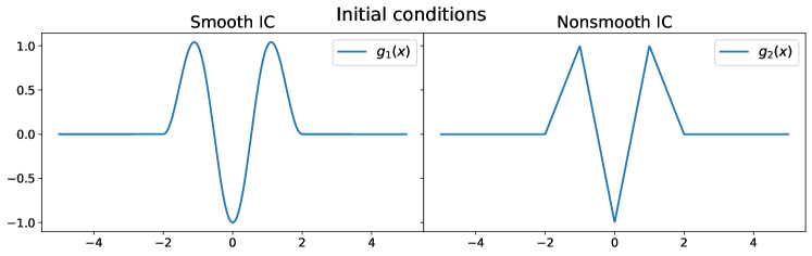
Figure 1. Initial conditions $g_{1}$ (left) and $g_{2}$ (right).

By Lemma 3.1 we implement the fractional Laplacian as

(4.2) $$-(-\Delta_{h})^{\frac{\sigma}{2}}U_{i}^{n}=\sum_{j\in\mathbb{Z}\backslash\{i\}}\kappa_{h,i-j}U_{j}^{n}-U_{i}^{n}\sum_{j\in\mathbb{Z}\backslash\{0\}}\kappa_{h,j}.$$

In dimension $N=1$ we have a simple formula for the weights [19, Theorem 1.1 a)]:

(4.3) $$\kappa_{h,j}=\frac{1}{h^{\sigma}}\frac{2^{\sigma}\Gamma(\frac{1+\sigma}{2})\Gamma(|j|-\tfrac{\sigma}{2})}{\sqrt{\pi}|\Gamma(-\frac{\sigma}{2})|\Gamma(|j|+1+\tfrac{\sigma}{2})}$$

Due to the rapid growth of the gamma function, infinity-over-infinity errors occur when calculating the factor $\frac{\Gamma(|j|-\frac{\sigma}{2})}{\Gamma(|j|+1+\frac{\sigma}{2})}$ directly for large $|j|$. To alleviate this, we use (i) asymptotic formulas like Stirling’s formula and/or (ii) logarithms

$$\exp\Big{[}\ln\big{(}\Gamma(|j|-\tfrac{\sigma}{2})\big{)}-\ln\big{(}\Gamma(|j|+1+\tfrac{\sigma}{2})\big{)}\Big{]}.$$

We truncate the sum in (4.2) at large $j$ to get a finite sum.

To get a finite computational domain, we truncate the domain, introducing artificial $0$-Dirichlet boundary conditions in the exterior. Spatial step size $h=2^{-5}$ and domain $[-20,20]$ ($[-20,20]\times[-20,20]$ in the 2D example) were used in the following simulations. To satisfy the CFL condition, temporal step size $\tau=c\cdot h^{\sigma}$ with $c=1,0.5,0.5,0.1$ were used for experiment 1a, 1b, 2 and 3 respectively.

4.1. Example 1: A degenerate diffusion equation in 1d

Here we solve (4.1) with the degenerate nonlinearity $F_{1}$.

(1a)  We first look at a fixed time $t=0.5$, two different initial conditions $g_{1},g_{2}$, and three different values of $\sigma$ ($\frac{1}{2},1,\frac{3}{2}$), see Figure 2. Compared to initial conditions (Figure 1), we observe that the positive peaks remain fixed while the negative peak has diffused/traveled upwards. The solution never becomes smooth.

Remark 4.1.

Because of the the nonlinearity $F_{1}$, the solution can only move/diffuse when the fractional Laplacian is positive and this only happens if the solution is ”convex enough”. At the positive peaks this is never the case, and the solution is stuck there. The problem is then equivalent to three independent boundary value problems with three independently diffusing solutions.

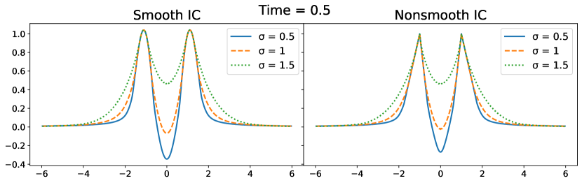
Figure 2. Experiment 1a.

(1b)  Now we study the time evolution of problem (4.1) with nonlinearity $F_{1}$ and non-smooth intial data $g_{1}$. We solve the problem at four different times and for three different values of $\sigma$ ($1,\frac{3}{2},2$), see Figure 3. As expected, we observe the strongest diffusion in the most convex regions.

Remark 4.2.

Short range diffusion become stronger the larger $\sigma$ is, but for long range diffusion it is the opposite. Therefore large $\sigma$ diffuse faster near peaks, but slower far away. This means that solutions in Figure 3 are not ordered, but rather they will reverse order far enough from the peaks.

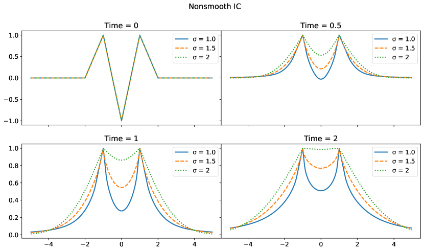
Figure 3. Experiment 1b.

4.2. Example 2: A degenerate diffusion equation in 2d

We solve

(4.4) $$\begin{split}U_{i,l}^{n+1}&=U_{i,l}^{n}+\tau\big{[}F_{1}\big{(}-(-\Delta_{h}^{x})^{\frac{1}{2}}U_{i,l}^{n}\big{)}+F_{2}\big{(}-(-\Delta_{h}^{y})^{\frac{1}{2}}U_{i,l}^{n}\big{)}\big{]},\\ U^{0}_{i,l}&=g_{1}\Big{(}\sqrt{x_{i}^{2}+y_{l}^{2}}\Big{)},\end{split}$$

where $(-\Delta_{h}^{x})^{\frac{1}{2}}$ and $(-\Delta_{h}^{y})^{\frac{1}{2}}$ denote (1d) $\frac{1}{2}$-Laplacians in $x$ and $y$ directions respectively. The initial condition is the 2d radially symmetric version of $g_{1}$. The solution at $t=1$ is shown Figure 4.

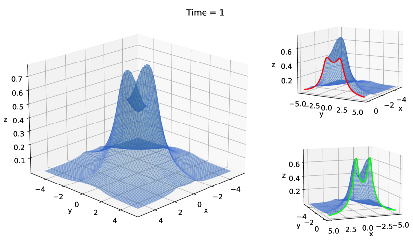
Figure 4. Experiment 2. The figures to the right show the solution for $x\leq 0$ (top) and $y\leq 0$ (bottom).

In this example no points are stuck and the solution diffuses in the whole domain. Observe from the red and green curves how the two different nonlinearities in (4.4) cause the solution to diffuse differently in the $x$ and $y$ directions.

4.3. Example 3: Limits of solutions as $\sigma\to 0$ and $\sigma\to 2$

It is well-known that $-(-\Delta)^{\frac{\sigma}{2}}\to\Delta$ as $\sigma\to 2^{-}$ and $-(-\Delta)^{\frac{\sigma}{2}}\to-Id$ as $\sigma\to 0^{+}$. Here we study numerically how solutions of (4.1) converge to solutions of the expected limiting equations. We consider nonlinearity $F_{1}$ and initial condition $g_{2}$, and the numerical solutions at $(t=10,\sigma\to 0)$ and $(t=0.1,\sigma\to 2)$ are shown in Figure 5.

Since the nonlinearity is $F_{1}$, the solution with $\sigma=0$ does not move after becoming nonnegative. The convergence is not so good as $\sigma\to 0$, but as $\sigma\to 2$ we see a linear rate of convergence in $L^{\infty}$ – see Table 1. The errors were calculated on the smaller domain $[-10,10]$ to avoid pollution from the artificial boundary conditions.

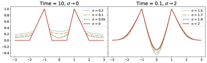
Figure 5. Experiment 3.

$2-\sigma$	Rel. error	rate
0.1	0.033	——
0.05	0.017	0.990
0.025	0.008	0.992
0.0125	0.004	0.994
0.00625	0.002	0.995

Table 1. Experiment 3 ($\sigma\to 2$). Relative $L^{\infty}$-errors at time $T=0.1$.

5. Extensions

5.1. On time discretizations

Different time discretizations can be considered as long as the resulting schemes are monotone. Here we discuss the $\theta$-method and the corresponding scheme for (1.5):

(5.1) $$U_{\mathbf{i}}^{n+1}=U_{\mathbf{i}}^{n}+\tau\Big{[}F\Big{(}-(1-\theta)(-\Delta_{h})^{\frac{\sigma}{2}}U_{\mathbf{i}}^{n}-\theta(-\Delta_{h})^{\frac{\sigma}{2}}U_{\mathbf{i}}^{n+1}\Big{)}+f_{\mathbf{i}}^{n}\Big{]}.$$

This scheme is fully implicit when $\theta=1$. It is explicit when $\theta=0$ and then the scheme coincides with (3.4). For other values, the scheme has both explicit and implicit terms. The scheme is monotone/$L^{\infty}$-stable under a modified CFL condition

(5.2) $$\quad(1-\theta)\tau\leq\frac{1}{L_{F}C_{\sigma}}h^{2\sigma},\quad\text{$C_{\sigma}$ and $L_{F}$ are given by Lemma \ref{lem::discr_fraclap_quadrature} and \ref{F1}}.$$

Comparison, $L^{\infty}$-stability, and consistency follow from similar arguments as for the explicit scheme (3.4), see Theorems 3.3, 3.4 and 3.8. Existence is no longer immediate, but follows from a fixed point argument (Banach) for each time step followed by an induction on the time steps – for a detailed proof see e.g. the arguments for [10, Theorem 3.1]. Convergence then follows as before:

Theorem 5.1.

Assume $\mathbf{(A1)}$, $\mathbf{(A2)}$, $\theta\in[0,1]$, CFL condition (5.7), and $u$ and $U_{h}$ solve (1.5) and (5.1) respectively. Then $U_{h}\to u$ locally uniformly as $h\rightarrow 0$.

Remark 5.2.

Only the fully implicit schemes $\theta=1$ have no CFL restriction here, see (5.2). Here the CFL condition is a condition to be monotone/$L^{\infty}$-stable. For linear (local) problems the case $\theta=\frac{1}{2}$ is known as the Cranck-Nicholson scheme. This scheme is von Neumann stable without any CFL condition, but to have stronger $L^{\infty}$-stability a CFL condition is also needed.

5.2. Equations with first order term

To explain how first order terms and convection phenomena modify our schemes and analysis, we consider the equation

(5.3) $$u_{t}-F\big{(}-(-\Delta)^{\frac{\sigma}{2}}u\big{)}+H(Du) =f(x,t),$$

where $H:\mathbb{R}^{N}\to\mathbb{R}$ satisfies

1. $|H(p_{1})-H(p_{2})|\leq L_{H}|p_{1}-p_{2}|$ for $p_{1},p_{2}\in\mathbb{R}^{N}$.

Under assumptions $\mathbf{(A1)}$, $\mathbf{(A2)}$, $\mathbf{(H1)}$, comparison and wellposedness of (5.3) holds as in Proposition 2.1. The proof remains the same since the results of [17] are very general and cover this case as well.

There are many ways to discretize the $H(Du)$-term to get a monotone numerical scheme for (5.3). Such schemes are often derived from monotone conservative schemes for scalar conservation laws like e.g. up-wind, Lax-Freidrich, Gudonov or Enquist-Osher type of schemes [24, 41, 40, 3]. For simplicity we consider an explicit scheme based on the Lax-Friedrich discretization [24, Section 2]:

(5.4) $$U_{\mathbf{i}}^{n+1}=U_{\mathbf{i}}^{n}+\tau\Big{[}F\big{(}-(-\Delta_{h})^{\frac{\sigma}{2}}U_{\mathbf{i}}^{n}\big{)}-H(\nabla^{\text{cd}}_{h}U_{\mathbf{i}}^{n})+h\,\Delta^{H}_{h}U_{\mathbf{i}}^{n}+f_{\mathbf{i}}^{n}\Big{]},$$

where for $k\in\{1,\cdots,n\}$,

$$\nabla^{\text{cd}}_{h}U=\big{(}D^{c}_{h,1}U,\cdots,D^{c}_{h,n}U\big{)}\quad\text{with}\quad D^{c}_{h,k}U(x)=\tfrac{U(x+he_{k})-U(x-he_{k})}{2h},$$

$$\Delta^{H}_{h}U=\sum_{k=1}^{N}L^{k}_{H}\tfrac{U(x+he_{k})-2U(x)+U(x-he_{k})}{h^{2}}\quad\text{with}\quad L^{k}_{H}=\tfrac{\|\partial_{k}H\|_{L^{\infty}}}{2}.$$

This scheme is monotone under the CFL condition

(5.5) $$\tau\leq\frac{1}{2h^{-1}L_{H}+L_{F}C_{\sigma}h^{-\sigma}}\qquad\text{where}\qquad L_{H}=\sum_{k=1}^{N}L^{k}_{H},$$

$L_{F}$ as in $\mathbf{(A1)}$, and $C_{\sigma}$ as in Lemma 3.1. A simpler sufficient condition is $\tau\leq C\min\{h,h^{\sigma}\}$ for a $C$ depending on $L_{H}$ and $L_{F}$.

Under CFL-condition (5.5) (and $\mathbf{(A1)}$, $\mathbf{(A2)}$, $\mathbf{(H1)}$), comparison for (5.4) holds as in Theorem 2, and then well-posedness and $L^{\infty}$-stability of (5.4) follow as before without change of proofs. Since $H(\nabla^{\text{cd}}_{h}\phi)+h\,\Delta^{H}_{h}\phi\to H(\nabla\phi)$ as $h\to 0$ for smooth functions $\phi$, the scheme is consistent and a version of Theorem 3.8 follows. By the method of half-relaxed limit we then get the following convergence result:

Theorem 5.3.

Assume $\mathbf{(A1)}$, $\mathbf{(A2)}$, $\mathbf{(H1)}$, CFL condition (5.5), and $u$ and $U_{h}$ solve (5.3) and (5.4) respectively. Then $U_{h}\to u$ locally uniformly to as $h\rightarrow 0$.

5.3. More general equations

Here we discuss how to extend our results to the nonlocal HJB/Isaacs equations (1.4). In view of e.g. [17, 34] sufficient conditions for strong comparison and well-posedness are given by

1. $c^{\alpha,\beta},a^{\alpha,\beta},b^{\alpha,\beta},f^{\alpha,\beta}$ are continuous in $\alpha,\beta,t,x$, and $a^{\alpha,\beta},c^{\alpha,\beta}\geq 0$, and

   $$\sup_{\alpha,\beta}\Big{\{}\|(a^{\alpha,\beta})^{\frac{1}{\sigma}}\|_{W^{1,\infty}},\|b^{\alpha,\beta}\|_{W^{1,\infty}},\|c^{\alpha,\beta}\|_{L^{\infty}},\|f^{\alpha,\beta}\|_{L^{\infty}}\Big{\}}\leq K.$$

The assumption on $a$ is best understood by looking at section 2.2. Assumption $\mathbf{(I1)}$ implies that the coefficients of the underlying SDE (2.1) are Lipschitz.

Consider now the following explicit scheme for (1.4),

(5.6) $$U_{\mathbf{i}}^{n+1}=U_{\mathbf{i}}^{n}+\tau\inf_{\beta\in\mathcal{B}}\sup_{\alpha\in\mathcal{A}}\big{\{}f^{\alpha,\beta}(x_{\mathbf{i}},t_{n})-c^{\alpha,\beta}(x_{\mathbf{i}},t_{n})U^{n}_{\mathbf{i}}+\mathcal{L}_{h}^{\alpha,\beta}U_{\mathbf{i}}^{n}\big{\}},$$

where

$$\mathcal{L}_{h}^{\alpha,\beta}U_{\mathbf{i}}^{n}= -a^{\alpha,\beta}(x_{\mathbf{i}},t_{n})(-\Delta_{h})^{\frac{\sigma}{2}}U_{\mathbf{i}}^{n}$$

$$\qquad+\sum_{k=1}^{N}\Big{(}b^{\alpha,\beta,+}_{k}(x_{\mathbf{i}},t_{n})D_{h,k}^{+}U_{\mathbf{i}}^{n}+b^{\alpha,\beta,-}_{k}(x_{\mathbf{i}},t_{n})D_{h,k}^{-}U_{\mathbf{i}}^{n}\Big{)},$$

and $D_{h,k}^{\pm}\phi(x)=\frac{\phi(x\pm he_{k})-\phi(x)}{h}$ and $b^{\alpha,\beta}=(b^{\alpha,\beta}_{1},\cdots,b^{\alpha,\beta}_{N})$. Here we have used an upwind approximation of the gradient term.

The scheme is monotone if for all gridpoints $(x_{\mathbf{i}},t_{n})$,

$$\tau\leq\frac{1}{h^{-1}\sum_{k=1}^{N}|b^{\alpha,\beta}_{k}(x_{\mathbf{i}},t_{n})|+a^{\alpha,\beta}(x_{\mathbf{i}},t_{n})C_{\sigma}h^{-\sigma}+c^{\alpha,\beta}(x_{\mathbf{i}},t_{n})}.$$

By $\mathbf{(I1)}$, a sufficient CFL condition is then given by

(5.7) $$\tau\leq\frac{1}{K\big{(}Nh^{-1}+C_{\sigma}h^{-\sigma}+1\big{)}},\qquad\text{where}\ K\ \text{is given by \ref{I1}}.$$

Under CFL condition (5.7) (and $\mathbf{(I1)}$, $\mathbf{(A2)}$), it is straight forward to show comparison of the scheme (c.f. Theorem 3.3). $L^{\infty}$-stability then follows by taking $\pm\big{(}\|u_{0}\|_{L^{\infty}}+t_{n}\sup_{\alpha,\beta}\|f^{\alpha,\beta}\|_{L^{\infty}}\big{)}$ as sub- and supersolutions. Again it is easy to verify that $\mathcal{L}_{h}^{\alpha,\beta}\phi\to\mathcal{L}^{\alpha,\beta}\phi$ as $h\to 0$ for any smooth bounded function $\phi$, and consistency a la Theorem 3.8 follow by similar arguments. By the half-relaxed limit method we then again have a convergence result.

Theorem 5.4.

Assume $\mathbf{(A2)}$, $\mathbf{(I1)}$, CFL condition (5.7), and $u$ and $U_{h}$ solve (1.4) and (5.6) respectively. Then $U_{h}\to u$ locally uniformly as $h\rightarrow 0$.

Remark 5.5.

Our results also apply when $\sigma$ depends on $\alpha,\beta$. In this case the differential operator in equation (1.4) is

$$\mathcal{L}^{\alpha,\beta}\phi=-a^{\alpha,\beta}(x,t)(-\Delta)^{\frac{1}{2}\sigma^{\alpha,\beta}}\phi(x)+b^{\alpha,\beta}(x,t)\cdot D\phi(x),$$

for $\sigma^{\alpha,\beta}\in(0,\bar{\sigma}]$ and $\bar{\sigma}<2$. In this case the CFL condition depends on the maximal order $\bar{\sigma}$ of the fractional Laplacian operators, $\tau\leq\frac{1}{K(Nh^{-1}+C_{\bar{\sigma}}h^{-\bar{\sigma}}+1)}$.

Remark 5.6.

Another extension is to consider equations involving powers of more general 2nd order elliptic differential operators $L$. Such powers are defined form formula (1.1) by replacing $\Delta$ with $L$, and the idea is to approximate by replacing $L$ by a finite difference approximation $L_{h}$. Such methods could be analysed in a similar way as we do here.

Declarations

Ethical approval

Not applicable.

Competing interests

The authors declare that they have no competing interests or other interests that might be perceived to influence the results and/or discussion reported in this paper.

Authors’ contributions

R.Ø.L. did the numerical simulations. All authors contributed equally to the rest of the paper.

Funding

I.C. was supported by DST-India funded INSPIRE faculty fellowship (IFA22-MA187). E.R.J. and R.Ø.L. received funding from the Research Council of Norway under Grant Agreement No. 325114 “IMod. Partial differential equations, statistics and data: An interdisciplinary approach to data-based modelling”.

Availability of data and materials

All the data have been generated by numerical simulations coded in Python. This code can be shared by R.Ø.L. upon request.

References

- [1] D. Applebaum. Lévy processes and stochastic calculus. Cambridge University Press, Cambridge, 116 (2) (2009).
- [2] M. Bardi and I. Capuzzo Dolcetta. Optimal control and viscosity solutions of Hamilton-Jacobi-Bellman equations. Birkauser, 1996.
- [3] M. Bardi and S. Osher. The nonconvex multidimensional Riemann problem for Hamilton-Jacobi equations. SIAM J. Math. Anal., 22 (2) (1991), 344–351.
- [4] G. Barles and C. Imbert. Second-order elliptic integro-differential equations: viscosity solutions’ theory revisited. Ann. Inst. H. Poincaré C Anal. Non Linéaire, 25 (3) (2008), 567–585.
- [5] G. Barles and P. E. Souganidis. Convergence of approximation schemes for fully nonlinear second order equations. Asymptotic Anal., 4 (1991), 271–283.
- [6] R. Bellman. Dynamic programming. Reprint of the 1957 edition. Princeton, 2010.
- [7] I. H. Biswas. On zero-sum stochastic differential games with jump-diffusion driven state: a viscosity solution framework. SIAM J. Control Optim. 50(4):1823–1858, 2012.
- [8] I. H. Biswas, I. Chowdhury and E. R. Jakobsen. On the rate of convergence for monotone numerical schemes for nonlocal Isaacs’ equations. SIAM J. Numer. Anal., 57 (2) (2019), 799–827.
- [9] I.H. Biswas, E.R. Jakobsen and K.H. Karlsen. Error estimates for a class of finite difference-quadrature schemes for fully nonlinear degenerate parabolic integro-PDEs. J. Hyperbolic Differ. Equ., 5 (1) (2008), 187–219.
- [10] I.H. Biswas, E.R. Jakobsen and K.H. Karlsen. Difference-quadrature schemes for nonlinear degenerate parabolic integro-PDE. SIAM J. Numer. Anal., 48 (3) (2010), 1110–1135.
- [11] A. Bonito and J. E. Pasciak. Numerical Approximation of fractional powers of elliptic operators. Math. Comp., 84 (295) (2015), 2083–2110.
- [12] J. F. Bonnans and H. Zidani. Consistency of generalized finite difference schemes for the stochastic HJB equation. SIAM J. Numer. Anal. 41(3) (2003), 1008–1021.
- [13] B. Bouchard, and N. Touzi. Discrete-time approximation and monte-carlo simulation of backward stochastic differential equations. Stoch. Process Their Appl. 111 (2) (2004), 175–206.
- [14] M. Boulbrachene and M. Haiour. The finite element approximation of Hamilton-Jacobi-Bellman equations. Comput. Math. Appl. 41 (7-8) (2001), 993–1007.
- [15] F. Camilli and M. Falcone. An approximation scheme for the optimal control of diffusion processes, RAIRO Modél. Math. Anal. Numér, 29 (1) (1995), 97–122.
- [16] F. Camilli and E. R. Jakobsen. A finite element like scheme for integro-partial differential Hamilton-Jacobi-Bellman equations, SIAM J. Numer. Anal., 47 (2009), 2407–2431.
- [17] E. Chasseigne and E. R. Jakobsen. On nonlocal quasilinear equations and their local limits, J. Differential Equations, 262 (6) (2017), 3759–3804.
- [18] I. Chowdhury and E. R. Jakobsen. Precise Error Bounds for Numerical Approximations of Fractional HJB Equations. Preprint 2023, arXiv:2308.16434.
- [19] O. Ciaurri, L. Roncal, P. R. Stinga, J. L. Torrea, and J. L. Varona. Nonlocal discrete diffusion equations and the fractional discrete Laplacian, regularity and applications. Adv. Math., 330 (2018), 688–738.
- [20] O. Ciaurri and L. Roncal and P. R. Stinga and J. L. Torrea and J. L. Varona Fractional discrete Laplacian versus discretized fractional Laplacian, (2023 Preprint, arXiv:1507.04986.
- [21] G. M. Coclite, O. Reichmann, and N. H. Risebro. A convergent difference scheme for a class of partial integro-differential equations modeling pricing under uncertainty, SIAM J. Numer. Anal., 54 (2016), 588–605.
- [22] R. Cont and P. Tankov. Financial modelling with jump processes. Chapman & Hall/CRC Financial Mathematics Series. Chapman & Hall/CRC, Boca Raton, FL, (2004), xvi+535 pp.
- [23] R. Cont and E. Voltchkova. A Finite Difference Scheme for Option Pricing in Jump Diffusion and Exponential Lévy Models. SIAM J. Numer. Anal. 43 (4) (2005), 1596–1626.
- [24] M. G. Crandall and P. L. Lions. Two approximations of solutions of Hamilton-Jacobi equations, Math. Comp. , 43 (1984), 1–19.
- [25] N. Cusimano, F. del Teso, and L. Gerardo-Giorda. Numerical approximations for fractional elliptic equations via the method of semigroups. ESAIM Math. Model. Numer. Anal. 54(3):751–774, 2020.
- [26] K. Debrabant and E.R. Jakobsen. Semi-Lagrangian schemes for linear and fully non-linear diffusion equations. Math. Comp., 82 (283)(2013), 1433–1462.
- [27] R. Dumitrescu, C. Reisinger, Y. Zhang. Approximation schemes for mixed optimal stopping and control problems with nonlinear expectations and jumps. Appl. Math. Optim. 83 (3) (2021), 1387–1429.
- [28] F. del Teso, J. Endal, and E.R. Jakobsen. Robust numerical methods for nonlocal (and local) equations of porous medium type. Part II: Schemes and experiments. SIAM J. Numer. Anal., 56 (6) (2018), 3611–3647.
- [29] M. Falcone and R. Ferretti. Semi-Lagrangian approximation schemes for linear and Hamilton-Jacobi equations. Society for Industrial and Applied Mathematics (SIAM), 2014.
- [30] W. H. Fleming and H. M. Soner. Controlled Markov processes and viscosity solutions, Springer, New York, 2006.
- [31] W. E, J. Han, and A. Jentzen. Solving high-dimensional partial differential equations using deep learning. Proc. Natl. Acad. Sci. USA 115(34) (2018), 8505–8510.
- [32] F. L. Hanson. Applied Stochastic Processes and Control for Jump-Diffusions: Modeling, Analysis and Computation. Society for Industrial and Applied Mathematics (SIAM), 2007.
- [33] H. Ishii and A Roch. Existence and uniqueness of viscosity solutions of an integro-differential equation arising in option pricing. SIAM J. Financial Math. 12 (2)(2021), 604–640.
- [34] E. R. Jakobsen and K. H. Karlsen. Continuous dependence estimates for viscosity solutions of integro-PDEs. J. Differential Equations, 212 (2) (2005), 278–318.
- [35] E. R. Jakobsen and K. H. Karlsen. A “maximum principle for semicontinuous functions” applicable to integro-partial differential equations. NoDEA Nonlinear Differential Equations Appl., 13 (2006), 137–165.
- [36] E. R. Jakobsen, K. H. Karlsen and C. La Chioma. Error estimates for approximate solutions to Bellman equations associated with controlled jump-diffusions. Numer. Math., 110 (2) (2008), 221–255.
- [37] H. J. Kushner and P. Dupuis. Numerical methods for stochastic control problems in continuous time. Springer, 2001.
- [38] Kwasnicki, M. Ten equivalent definitions of the fractional Laplace operator. Fract. Calc. Appl. Anal. 20(1):7–51, 2017.
- [39] O. Lepsky. Spectral Viscosity Approximations to Hamilton–Jacobi Solutions. SIAM J. Numer. Anal. 38 (5) (2000), 1439–1453.
- [40] S. Osher and J. A. Sethian. Fronts propagating with curvature-dependent speed: algorithms based on Hamilton-Jacobi formulations. J. Comput. Phys. 79 (1) (1988), no.1, 12–49.
- [41] S. Osher and C. W. Shu. High-order essentially nonoscillatory schemes for Hamilton-Jacobi equations. SIAM J. Numer. Anal. 28 (4) (1991), 907–922.
- [42] B. Øksendal and A. Sulem. Applied stochastic control of jump diffusions. Springer, Cham, 2019.
- [43] C. Reisinger, Y. Zhang. A penalty scheme and policy iteration for nonlocal HJB variational inequalities with monotone nonlinearities. Comput. Math. Appl. 93 (2021), 199–213.
- [44] X. Ros-Oton and M. Weidner. Obstacle problems for nonlocal operators with singular kernels. Preprint arXiv:2308.01695.
- [45] I. Smears and E. Süli. Discontinuous Galerkin finite element approximation of nondivergence form elliptic equations with Cordès coefficients. SIAM J. Numer. Anal. 51 (4) (2013), 2088–2106.
- [46] P. E. Souganidis. Approximation schemes for viscosity solutions of Hamilton-Jacobi equations, J. Differential Equations, 59 (1) (1985), 1–43.
- [47] F. del Teso and E. R. Jakobsen. A convergent finite difference-quadrature scheme for the porous medium equation with nonlocal pressure, Preprint, arXiv:2303.05168 [math.NA], (2023).