Dynamical heterogeneities of thermal creep in pinned interfaces
Abstract
Disordered systems under applied loading display slow creep flows at finite temperature, which can lead to the material rupture. Renormalization group arguments predicted that creep proceeds via thermal avalanches of activated events. Recently, thermal avalanches were argued to control the dynamics of liquids near their glass transition. Both theoretical approaches are markedly different. Here we provide a scaling description that seeks to unify dynamical heterogeneities in both phenomena, confirm it in simple models of pinned elastic interfaces, and discuss its experimental implications.
Introduction
The physical properties of a material are often controlled by the interfaces embedded in it. This is the case for dislocations in crystalline materials Miguel et al. (2001); Madec et al. (2003); Zaiser (2006), crack fronts in fracture Bouchaud (1997), frictional interfaces Scholz (1998), or domain walls in magnets Zapperi et al. (1998). Pinned by impurities, they dramatically increase the material’s strength, toughness, or hysteresis. At the critical force (or stress, or magnetic field) , the interfaces undergo a depinning transition Kardar (1998); Fisher (1998) and move via large reorganizations, called avalanches. Their maximal linear extent diverges approaching the critical point, and their size is power law distributed, . Moreover, the interface shape is a self-similar shape with a roughness exponent . These exponents are now well understood and related by scaling relations summarized in Table 1.
The dynamics below , in the so-called creep regime, is more controversial. Here, the motion is controlled by the thermal activation over the pinning potential Ferrero et al. (2021). Creep is fundamental for a variety of phenomena, ranging from the failure of materials Leocmach et al. (2014); Divoux et al. (2011); Siebenbürger et al. (2012); Rosti et al. (2010) to the rupture of frictional interfaces and faults Baumberger et al. (1994); Bureau et al. (2001); Bar-Sinai et al. (2013); Harris (2017); Vincent-Dospital et al. (2020). In Chauve et al. (2000), a study of pinned interfaces based on the functional renormalization group (FRG), predicted the existence of two distinct length scales:
(i) The first length, , corresponds to the extent of the elementary excitations. Elementary excitations correspond to the minimal motion in the direction of the applied force that brings the interface to a new local minimum with smaller energy. They can be treated as being irreversible, since the probability of going backward once an excitation is triggered is small. grows as when the force vanishes. Below this scale, the interface is at equilibrium with a roughness exponent Ioffe and Vinokur (1987); Nattermann (1987); Agoritsas et al. (2012).
(ii) The second, much larger length, , identifies with the cut-off of the thermal avalanches induced by the interaction between elementary excitations. Below this length, the roughness exponent is and avalanches are depinning-like. This cut-off also diverges, as
| (1) |
The FRG equations cannot be solved exactly. In Chauve et al. (2000) an ansatz was proposed that leads to and 111 The depinning exponent controls, at zero temperature, the velocity of the interface, which vanishes as at . The equilibrium exponent appears in the creep formula . This behaviour has been confirmed experimentally in Lemerle et al. (1998). .
Efficient optimization algorithms at vanishing temperature have studied the case of a one-dimensional domain wall moving in a medium in two dimensions Kolton et al. (2006, 2009); Ferrero et al. (2017). They confirmed the scaling of , the crossover of the roughness exponents from equilibrium to depinning, as well as the presence of thermal depinning avalanches. Experiments on a one-dimensional domain wall in a ferromagnetic film showed the validity of the creep formula for the wall velocity, which is an indirect check for the scaling of Lemerle et al. (1998); Metaxas et al. (2007). Recently, depinning thermal avalanches have been observed via Magneto-optic Kerr effect (MOKE) techniques Grassi et al. (2018); Durin et al. (2023) and in crumpled paper Lahini et al. (2023); Shohat et al. (2023). However, the determination of remains an open problem – finite temperature simulations using Langevin dynamics were inconclusive Kolton et al. (2009).
Recently, it was proposed that the concept of thermal avalanches extends beyond driven systems, and explains the dynamical heterogeneities observed in supercooled liquids Tahaei et al. (2023). In that case, it was argued that with , whereby is an exponent that characterizes the distribution of excitations Lin et al. (2014); Lin and Wyart (2016). In the context of the depinning transition . In two dimensions, this inequality was found to be saturated in mesoscopic models of liquids Tahaei et al. (2023). Arguments in Tahaei et al. (2023) should also go through in the depinning context, yet the bound is much below the FRG predictions.
In this Letter, we propose a scaling theory of dynamical heterogeneities for both phenomena. We introduce a stylized model for creep of depinning interfaces, where the optimized elementary excitations are coarse-grained at the scale of a single block. At zero temperature, the model reduces to the cellular automata used to study the depinning transition and its exponents. At finite temperature, a similar model was discussed in Vandembroucq et al. (2004); Purrello et al. (2017), but not used to study the creep regime. We provide theoretical arguments indicating that
| (2) |
both for depinning and for the glass transition (see below for a definition of in the latter case). Moreover, we argue that in the depinning case, the relationship between the age of an avalanche and its spatial extent follows, as for liquids Tahaei et al. (2023):
| (3) |
where is a characteristic timescale at which a fraction of the interface has moved. We find that all our predictions hold quantitatively in a mesoscopic model of depinning.
| Name | Expression | Scaling | Value |
|---|---|---|---|
Model
We model an elastic interface in a mesoscopic manner, coarse-grained on the excitation scale . Such a model is the basis of both our theoretical arguments, and of our numerical study below. The system is a lattice of blocks. The block is characterized by an applied force (the sum of the driving force and elastic forces coming from neighboring blocks), and by a yielding threshold . Its stability is governed by the distance to yielding , corresponding to an activation barrier with some . Our arguments below do not depend on the value of .
At a finite temperature (that we express in the units of the Boltzmann constant ), the time to failure of a block is exponentially distributed . Here the characteristic time is if and otherwise, where is a fixed microscopic timescale. After failure, the force drops to a small random value, and a fresh value of the yield force is sampled from a fixed distribution. The force drop is redistributed equally to the nearest neighboring blocks, as follows from the presence of elastic interactions. Finally, the position of the interface at block , , is increased by the value of the force drop (using an elastic constant of one).
It is well known that such a cellular automaton has a threshold force , such that if the applied force is larger than a depinning threshold , the dynamics does not stop even if . In our arguments we consider that and , while numerics are performed with , and . We express forces in units of average yield threshold , time in units of , temperature in units of , and length in units of the lattice spacing. Further numerical details are specified in Appendix A.
Extremal dynamics
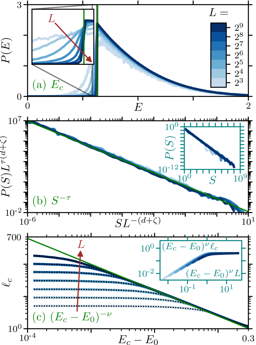
For finite , if is vanishingly small, the site with the smallest activation barrier always relaxes first. It is an example of extremal dynamics noted here as . It is well studied in the context of self-organized criticality Paczuski et al. (1996); Vandembroucq et al. (2004); Purrello et al. (2017). As , the distribution of energy barriers must have a compact support, and be zero below a force-dependent value 222 The probability to trigger to instability a block with is vanishing as . Because the number of blocks is extensive in the energy range , can never be the extremal, minimum, energy among all blocks. . must grow as the applied force decreases, and vanishes at the depinning threshold . Thus in the case considered here one has .
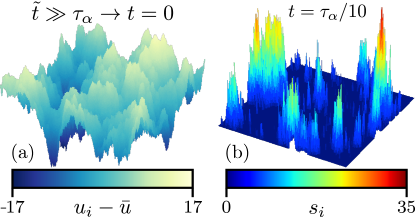
For finite , in not sharply defined but displays sample to sample fluctuations illustrated in Fig. 1a. After averaging the distribution of over various configurations, has a standard deviation that decays algebraically with as
| (4) |
Note that for elastoplastic models used to study the glass transition Tahaei et al. (2023); Ozawa and Biroli (2023), Eq. 4 defines , which will take a different value than for the elastic interface.
For extremal dynamics, avalanches can be defined as a sequence of fast events where the most unstable site always satisfies , where is some chosen threshold Paczuski et al. (1996); Purrello et al. (2017). In the thermodynamic limit, it is clear that the sequence never stops if . It is critical at , and falls in the depinning universality class with , with a cut-off at finite . It is confirmed in Fig. 1b with exponents indeed given by Table 1 (see Appendix C for an illustration on the method and Appendix B for further supporting measurements).
For , avalanches will be cut off once they reach some spatial extent . must be the length scale where the local fluctuations of the gap are of order of the difference : clearly, on a smaller scale, this difference is irrelevant. Using Eq. 4 yields:
| (5) |
This result is confirmed numerically in Fig. 1c. Here, we define the linear extent of an avalanche as , where the ‘area’ is the number of sites that yielded at least once. The cut-off is then defined as the ratio of moments where the average is made over avalanches. We define to provide the best collapse of Eq. 5 in the inset of Fig. 1c.
Finite temperature
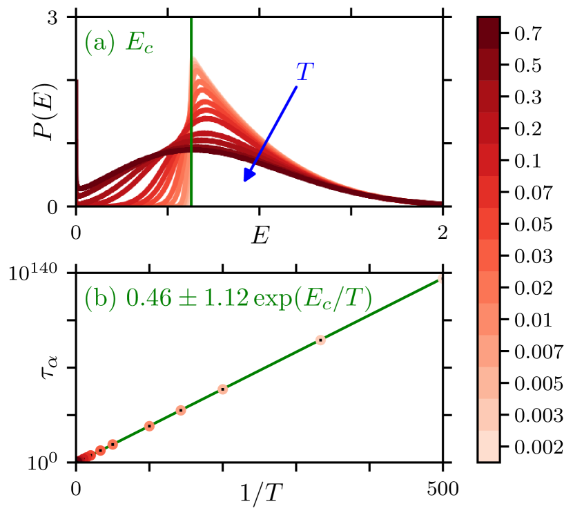
At a finite but small enough (to be specified below) temperature and fixed , the above picture remains true, but the dynamics now occur on a finite time scale. The duration of an avalanche defined with threshold will be of order of the longest waiting time between events within it, of order , thus . The largest avalanches filling up the system occur on some time . We extract numerically as the time at which half of the system fails at least once, which indeed is proportional to as we test in Appendix E. Injecting these definitions in Eq. 5, one gets for :
| (6) |
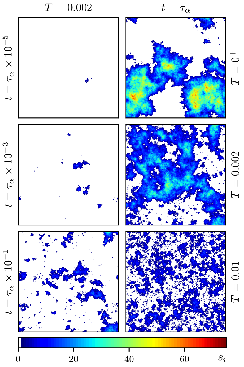
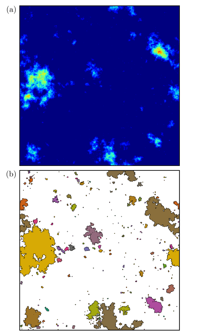
A similar argument was proposed for supercooled liquids, and matched the growth of dynamical heterogeneities with time in molecular dynamics observations well Tahaei et al. (2023). This prediction can be tested in the depinning case by considering the pattern of relaxations occurring in some time interval , as illustrated in the left panel of Fig. 2. We extract avalanches from these figures as connected clusters, and . Here the average is made on all clusters observed at temperature in intervals of duration , and the extent is defined as above (the square root of the cluster area in our numerics). Our prediction is confirmed in Fig. 3 (see Appendix C for illustration of the method, and Appendix D for further supporting measurements on both the avalanche exponents as well as our prediction in Eq. 6).
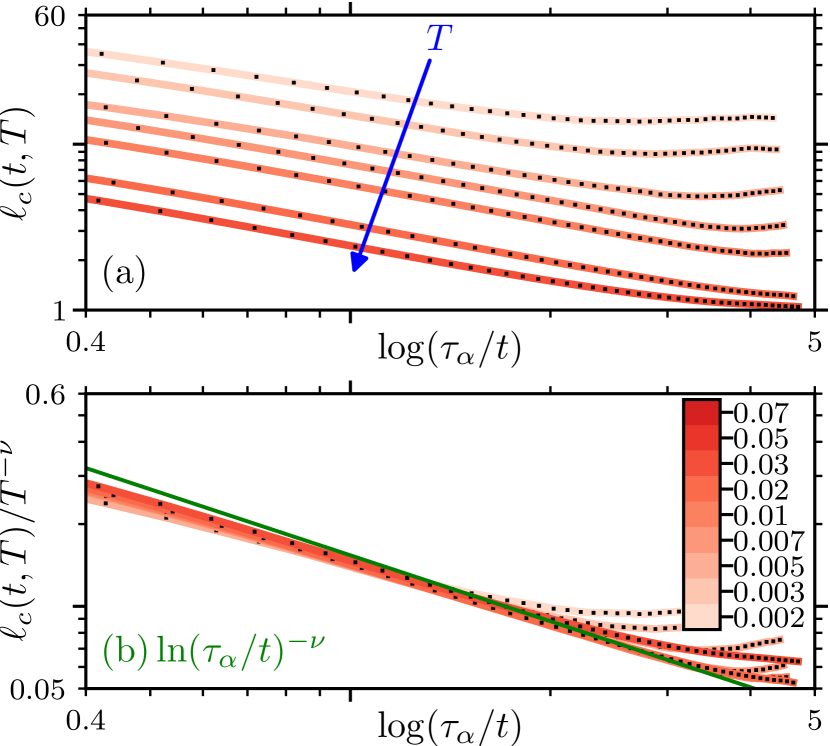
We now focus on our central question: the correlation length in an infinite system. The right panel of Fig. 2 shows the interface motion during a time interval of (where half of the sites relaxed), for different temperatures. Clearly, the dynamics is more and more correlated under cooling. To explain these observations, we perform a finite size scaling argument. Consider an infinite system cuts into subsystems of size . The fluctuations of the gaps in different subsystems follows . If , these subsystems relax essentially at the same speed, while if their pace is very different. Thus, dynamical heterogeneities should exist up to a length such , implying:
| (7) |
Note that this result also identifies with the avalanche extent occurring on a timescale , according to Eq. 6.
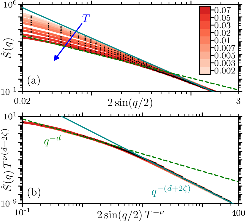
In the case of elastic interfaces, dynamical correlations also affect the structural correlations in the interface geometry. In particular, we expect the depinning roughness exponent to hold up to a scale . Above this length scale, avalanches become independent and they are randomly triggered. As in the Edwards-Wilkinson model, the roughness becomes for and logarithmic for .
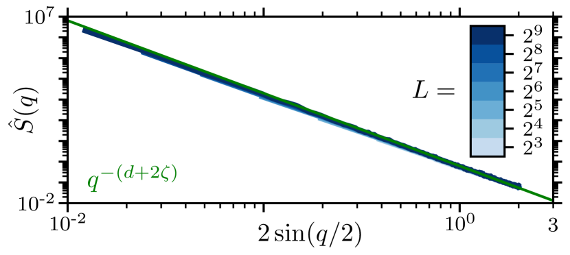
This prediction is verified by considering the structure factor , with the position of the interface at location ; is its Fourier transform and the Euclidean norm of wave vector . The average is taken on independent snapshots taken at random times. For a self-affine interface with roughness exponent , the structure factor scales as (e.g. Ramasco et al. (2000); Schmittbuhl et al. (1995)) and as for a logarithmic roughness. The crossover between the two regimes occurs at a scale . We verify such scaling in Fig. 4a and find that the crossover scale from Eq. 7 indeed collapses data for different in Fig. 4b.
Conclusion
We have provided a description of thermal avalanches which may characterize dynamical heterogeneities in both the creep flows of pinned interfaces and in supercooled liquids. As proposed for liquids Tahaei et al. (2023), we argued in the context of depinning that the growth of avalanche size with time is logarithmic, and tested this prediction in a simple model. This prediction could be tested in experiments monitoring the domain wall dynamics Grassi et al. (2018); Durin et al. (2023) or by the motion of dislocations in crystalline materials Rodney et al. (2023).
Our central prediction concerns the correlation length . The scaling of the correlation length differs from the FRG prediction of Chauve et al. (2000). The latter was obtained from an Ansatz solution, it will be interesting to see if our prediction can be derived from the original FRG equations. It will also be important to verify Eq. 7 from direct simulations of a continuous elastic line at finite temperature, or in experiments by recording the dynamics at different temperatures using a cryostat, as in Grassi et al. (2018).
For supercooled liquids, we have argued that , which should be, in general, distinct from the bound proposed in Tahaei et al. (2023). In two dimensions, an elastoplastic model of the glass transition predicted and 333 is noted in that reference, where it is extracted from Eq. 5., and both predictions are consistent with the observation . We expect the similarity between these exponents to be a coincidence, which for example does not occur for the pinned interface investigated here. We expect this similarity to disappear in the practically relevant case of three-dimensional liquids. This point can now be tested in three-dimensional elastoplastic models, by extracting both exponents and . Measuring would lead to quantitative prediction for the temporal or thermal behavior of dynamical heterogeneities that could be tested in experiments Weeks et al. (2000).
Acknowledgements
E. El Sergany is thanked for exploratory numerical tests, and L. Berthier, G. Biroli, C. Brito, C. Gavazzoni, D. Korchinski, W. Ji, Y. Lahini, M. Müller, M. Ozawa, M. Pica Ciamarra, M. Popović, D. Shoat, and A. Tahei for discussions. T.G. acknowledges support from the Swiss National Science Foundation (SNSF) by the SNSF Ambizione Grant PZ00P2_185843. M.W. acknowledges support from the Simons Foundation Grant (No. 454953 Matthieu Wyart).
References
- Miguel et al. [2001] M. C. Miguel, A. Vespignani, S. Zapperi, J. Weiss, and J.-R. Grasso. Intermittent dislocation flow in viscoplastic deformation. Nature, 410(6829):667–671, 2001. 10.1038/35070524. arxivid: cond-mat/0105069.
- Madec et al. [2003] R. Madec, B. Devincre, L. Kubin, T. Hoc, and D. Rodney. The Role of Collinear Interaction in Dislocation-Induced Hardening. Science, 301(5641):1879–1882, 2003. 10.1126/science.1085477.
- Zaiser [2006] M. Zaiser. Scale invariance in plastic flow of crystalline solids. Adv. Phys., 55(1–2):185–245, 2006. 10.1080/00018730600583514.
- Bouchaud [1997] E. Bouchaud. Scaling properties of cracks. J. Phys. Condens. Matter, 9(21):4319–4344, 1997. 10.1088/0953-8984/9/21/002.
- Scholz [1998] C. H. Scholz. Earthquakes and friction laws. Nature, 391(6662):37–42, 1998. 10.1038/34097.
- Zapperi et al. [1998] S. Zapperi, P. Cizeau, G. Durin, and H. E. Stanley. Dynamics of a ferromagnetic domain wall: Avalanches, depinning transition, and the Barkhausen effect. Phys. Rev. B, 58(10):6353–6366, 1998. 10.1103/PhysRevB.58.6353. arxivid: cond-mat/9803253.
- Kardar [1998] M. Kardar. Nonequilibrium dynamics of interfaces and lines. Phys. Rep., 301(1–3):85–112, 1998. 10.1016/S0370-1573(98)00007-6. arxivid: cond-mat/9704172.
- Fisher [1998] D. S. Fisher. Collective transport in random media: From superconductors to earthquakes. Phys. Rep., 301(1–3):113–150, 1998. 10.1016/S0370-1573(98)00008-8. arxivid: cond-mat/9711179.
- Ferrero et al. [2021] E. E. Ferrero, L. Foini, T. Giamarchi, A. B. Kolton, and A. Rosso. Creep Motion of Elastic Interfaces Driven in a Disordered Landscape. Annu. Rev. Condens. Matter Phys., 12(1):111–134, 2021. 10.1146/annurev-conmatphys-031119-050725.
- Leocmach et al. [2014] M. Leocmach, C. Perge, T. Divoux, and S. Manneville. Creep and Fracture of a Protein Gel under Stress. Phys. Rev. Lett., 113(3):038303, 2014. 10.1103/PhysRevLett.113.038303. arxivid: 1401.8234.
- Divoux et al. [2011] T. Divoux, C. Barentin, and S. Manneville. From stress-induced fluidization processes to Herschel-Bulkley behaviour in simple yield stress fluids. Soft Matter, 7(18):8409, 2011. 10.1039/C1SM05607G. arxivid: 1012.0693.
- Siebenbürger et al. [2012] M. Siebenbürger, M. Ballauff, and Th. Voigtmann. Creep in Colloidal Glasses. Phys. Rev. Lett., 108(25):255701, 2012. 10.1103/PhysRevLett.108.255701.
- Rosti et al. [2010] J. Rosti, J. Koivisto, L. Laurson, and M. J. Alava. Fluctuations and Scaling in Creep Deformation. Phys. Rev. Lett., 105(10):100601, 2010. 10.1103/PhysRevLett.105.100601. arxivid: 1007.4688.
- Baumberger et al. [1994] T. Baumberger, F. Heslot, and B. Perrin. Crossover from creep to inertial motion in friction dynamics. Nature, 367(6463):544–546, 1994. 10.1038/367544a0.
- Bureau et al. [2001] L. Bureau, T. Baumberger, and C. Caroli. Jamming creep of a frictional interface. Phys. Rev. E, 64(3):031502, 2001. 10.1103/PhysRevE.64.031502. arxivid: cond-mat/0101357.
- Bar-Sinai et al. [2013] Y. Bar-Sinai, R. Spatschek, E. A. Brener, and E. Bouchbinder. Instabilities at frictional interfaces: Creep patches, nucleation, and rupture fronts. Phys. Rev. E, 88(6):060403, 2013. 10.1103/PhysRevE.88.060403. arxivid: 1306.3658.
- Harris [2017] R. A. Harris. Large earthquakes and creeping faults. Rev. Geophys., 55(1):169–198, 2017. 10.1002/2016RG000539.
- Vincent-Dospital et al. [2020] T. Vincent-Dospital, R. Toussaint, S. Santucci, L. Vanel, D. Bonamy, L. Hattali, A. Cochard, E. G. Flekkøy, and K. J. Måløy. How heat controls fracture: The thermodynamics of creeping and avalanching cracks. Soft Matter, 16(41):9590–9602, 2020. 10.1039/D0SM01062F. arxivid: 1905.07180.
- Chauve et al. [2000] P. Chauve, T. Giamarchi, and P. Le Doussal. Creep and depinning in disordered media. Phys. Rev. B, 62(10):6241–6267, 2000. 10.1103/PhysRevB.62.6241. arxivid: cond-mat/0002299.
- Ioffe and Vinokur [1987] L. B. Ioffe and V. M. Vinokur. Dynamics of interfaces and dislocations in disordered media. J. Phys. C, 20(36):6149–6158, 1987. 10.1088/0022-3719/20/36/016.
- Nattermann [1987] T. Nattermann. Interface Roughening in Systems with Quenched Random Impurities. Europhys. Lett., 4(11):1241–1246, 1987. 10.1209/0295-5075/4/11/005.
- Agoritsas et al. [2012] E. Agoritsas, V. Lecomte, and T. Giamarchi. Disordered elastic systems and one-dimensional interfaces. Phys. B, 407(11):1725–1733, 2012. 10.1016/j.physb.2012.01.017. arxivid: 1111.4899.
- Lemerle et al. [1998] S. Lemerle, J. Ferré, C. Chappert, V. Mathet, T. Giamarchi, and P. Le Doussal. Domain Wall Creep in an Ising Ultrathin Magnetic Film. Phys. Rev. Lett., 80(4):849–852, 1998. 10.1103/PhysRevLett.80.849.
- Kolton et al. [2006] A. B. Kolton, A. Rosso, T. Giamarchi, and W. Krauth. Dynamics below the Depinning Threshold in Disordered Elastic Systems. Phys. Rev. Lett., 97(5):057001, 2006. 10.1103/PhysRevLett.97.057001. arxivid: cond-mat/0603297.
- Kolton et al. [2009] A. B. Kolton, A. Rosso, T. Giamarchi, and W. Krauth. Creep dynamics of elastic manifolds via exact transition pathways. Phys. Rev. B, 79(18):184207, 2009. 10.1103/PhysRevB.79.184207. arxivid: 0902.4557.
- Ferrero et al. [2017] E. E. Ferrero, L. Foini, T. Giamarchi, A. B. Kolton, and A. Rosso. Spatiotemporal Patterns in Ultraslow Domain Wall Creep Dynamics. Phys. Rev. Lett., 118(14):147208, 2017. 10.1103/PhysRevLett.118.147208. arxivid: 1604.03726.
- Metaxas et al. [2007] P. J. Metaxas, J. P. Jamet, A. Mougin, M. Cormier, J. Ferré, V. Baltz, B. Rodmacq, B. Dieny, and R. L. Stamps. Creep and Flow Regimes of Magnetic Domain-Wall Motion in Ultrathin Pt / Co / Pt Films with Perpendicular Anisotropy. Phys. Rev. Lett., 99(21):217208, 2007. 10.1103/PhysRevLett.99.217208. arxivid: cond-mat/0702654.
- Grassi et al. [2018] M. P. Grassi, A. B. Kolton, V. Jeudy, A. Mougin, S. Bustingorry, and J. Curiale. Intermittent collective dynamics of domain walls in the creep regime. Phys. Rev. B, 98(22):224201, 2018. 10.1103/PhysRevB.98.224201. arxivid: 1804.09572.
- Durin et al. [2023] G. Durin, V. M. Schimmenti, M. Baiesi, A. Casiraghi, A. Magni, L. Herrera-Diez, D. Ravelosona, L. Foini, and A. Rosso. Earthquake-like dynamics in ultrathin magnetic film. arXiv preprint: 2309.12898, 2023. 10.48550/arXiv.2309.12898.
- Lahini et al. [2023] Y. Lahini, S. M. Rubinstein, and A. Amir. Crackling Noise during Slow Relaxations in Crumpled Sheets. Phys. Rev. Lett., 130(25):258201, 2023. 10.1103/PhysRevLett.130.258201.
- Shohat et al. [2023] D. Shohat, Y. Friedman, and Y. Lahini. Logarithmic aging via instability cascades in disordered systems. Nat. Phys., 19(12):1890–1895, 2023. 10.1038/s41567-023-02220-2. arxivid: 2306.00567.
- Tahaei et al. [2023] A. Tahaei, G. Biroli, M. Ozawa, M. Popović, and M. Wyart. Scaling Description of Dynamical Heterogeneity and Avalanches of Relaxation in Glass-Forming Liquids. Phys. Rev. X, 13(3):031034, 2023. 10.1103/PhysRevX.13.031034. arxivid: 2305.00219.
- Lin et al. [2014] J. Lin, A. Saade, E. Lerner, A. Rosso, and M. Wyart. On the density of shear transformations in amorphous solids. EPL Europhys. Lett., 105(2):26003, 2014. 10.1209/0295-5075/105/26003.
- Lin and Wyart [2016] J. Lin and M. Wyart. Mean-Field Description of Plastic Flow in Amorphous Solids. Phys. Rev. X, 6(1):011005, 2016. 10.1103/PhysRevX.6.011005.
- Vandembroucq et al. [2004] D. Vandembroucq, R. Skoe, and S. Roux. Universal depinning force fluctuations of an elastic line: Application to finite temperature behavior. Phys. Rev. E, 70(5):051101, 2004. 10.1103/PhysRevE.70.051101. arxivid: cond-mat/0311485.
- Purrello et al. [2017] V. H. Purrello, J. L. Iguain, A. B. Kolton, and E. A. Jagla. Creep and thermal rounding close to the elastic depinning threshold. Phys. Rev. E, 96(2):022112, 2017. 10.1103/PhysRevE.96.022112. arxivid: 1704.01489.
- Paczuski et al. [1996] M. Paczuski, S. Maslov, and P. Bak. Avalanche dynamics in evolution, growth, and depinning models. Phys. Rev. E, 53(1):414–443, 1996. 10.1103/PhysRevE.53.414. arxivid: adap-org/9510002.
- Ozawa and Biroli [2023] M. Ozawa and G. Biroli. Elasticity, Facilitation, and Dynamic Heterogeneity in Glass-Forming Liquids. Phys. Rev. Lett., 130(13):138201, 2023. 10.1103/PhysRevLett.130.138201. arxivid: 2209.08861.
- Ramasco et al. [2000] J. J. Ramasco, J. M. López, and M. A. Rodríguez. Generic Dynamic Scaling in Kinetic Roughening. Phys. Rev. Lett., 84(10):2199–2202, 2000. 10.1103/PhysRevLett.84.2199. arxivid: cond-mat/0001111.
- Schmittbuhl et al. [1995] J. Schmittbuhl, J.-P. Vilotte, and S. Roux. Reliability of self-affine measurements. Phys. Rev. E, 51(1):131–147, 1995. 10.1103/PhysRevE.51.131.
- Rodney et al. [2023] D. Rodney, P.-A. Geslin, S. Patinet, V. Démery, and A. Rosso. Does the Larkin length exist? working paper or preprint, December 2023. URL https://hal.science/hal-04355482.
- Weeks et al. [2000] E. R. Weeks, J. C. Crocker, A. C. Levitt, A. Schofield, and D. A. Weitz. Three-Dimensional Direct Imaging of Structural Relaxation Near the Colloidal Glass Transition. Science, 287(5453):627–631, 2000. 10.1126/science.287.5453.627.
Supplementary material
Appendix A Model details
We list the remaining details of our model.
Interactions
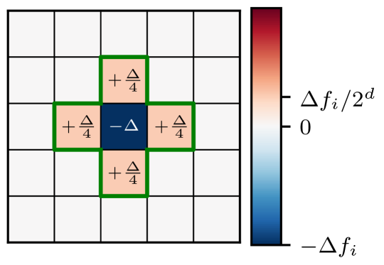
The elastic interactions are such that if a block fails, it loses its force up to a small random number, , such that with . Thereby, is a random number distributed normally as , whereby the notation is such that its mean in and its standard deviation is . The position of the interface (using an elastic constant of one). The force drop of the failing block is entirely redistributed to the nearest neighbors, , as shown in Fig. S1 for our case in dimensions. Consequently, the applied force is constant at all times.
Forces
We take . We estimated by driving the interface with a weak spring. Furthermore, the yield threshold of each block is random according to a normal distribution , truncated at .
Preparation
The force in each block is initialized random according to a normal distribution, , which is convoluted once with the elastic kernel from Fig. S1. Any unstable block is then failed, and the stress is redistributed to its nearest neighbors. This is repeated until all blocks are stable. The system is then driven for at least steps at the temperature used for the measurement (or using “extremal dynamics” if ).
Appendix B Roughness exponents
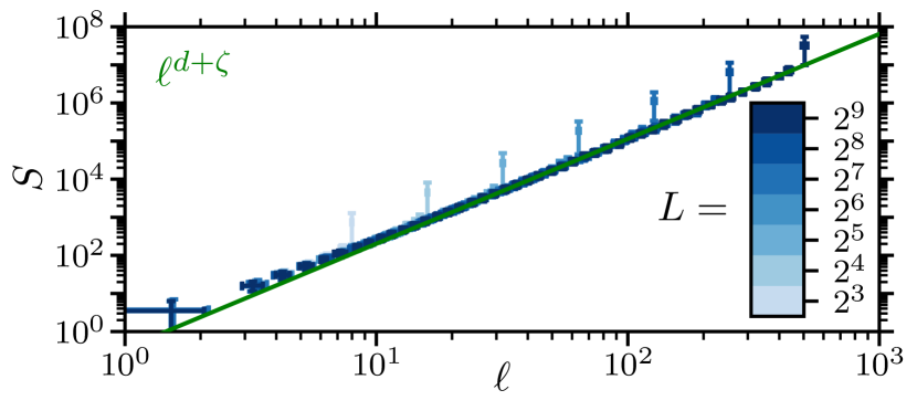
The geometry of avalanches is consistent with a roughness exponent , with its value predicted by the depinning theory recalled in Table 1. We support this by two measurements at . First, we measure the roughness of the interface at random snapshots in the steady state. In particular, we measure the structure factor and find that it is consistent with (see main text), as shown in Fig. S2 (see e.g. Ramasco et al. [2000], Schmittbuhl et al. [1995] for discussions on the use of the structure factor to measure the roughness exponent of a self-affine interface). Second, we measure the fractal dimension of avalanches. We define avalanches as a sequence for which the activation barrier with . We plot the total number of fails in each sequence, (the ‘duration’ of each sequence), as a function of spatial extent (with the number of unique blocks in the sequence) in Fig. S3. We find that it is consistent with .
Appendix C Avalanche identification
Extremal dynamics
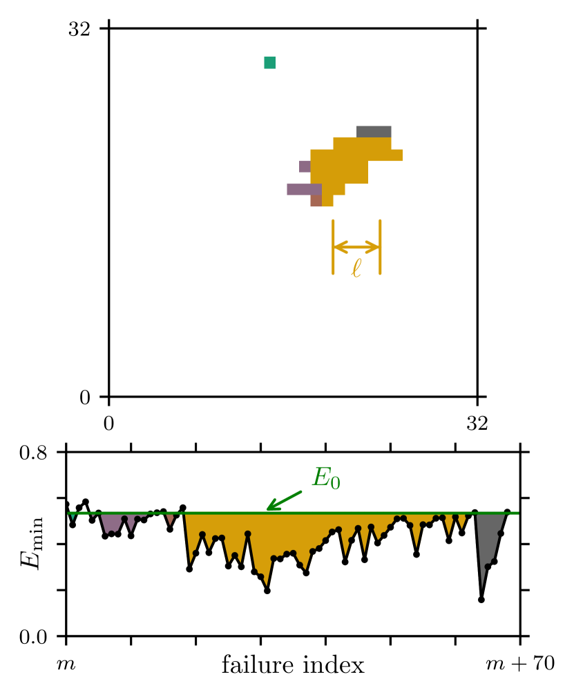
We measure a sequence of failures starting from a random snapshot somewhere in the steady state (for which each block already yielded many times since preparation). We record the activation barrier and the spatial location of each failure. We define avalanches as sequences of failures for which , with some threshold. We illustrate this in Fig. S4 for a small subset of failures in a small system. These avalanches are characterized by , the total number of failures in sequence, and the number of blocks that had at least one failure since the beginning of the avalanche. Then, is used as a proxy of the linear extent of the avalanche.
Finite temperature
We again measure avalanches starting from an ensemble of independent snapshots at random times in the steady state. As an example, we show a snapshot of the position of the interface at a random time in the steady state in Fig. S5a. Starting from this snapshot which marks a duration we record the number of times that each block fails at different times (see example in Fig. S5b).
Individual avalanches are then identified as connected clusters of blocks that failed at least once. An example is shown in Fig. S6. Fig. S6a shows a projection of Fig. S5 with the same color bar. The identified clusters are shown in Fig. S6b, whereby each cluster is assigned a different color, and a black outline is drawn around each cluster. The connectedness of clusters is decided using the same nearest-neighbor kernel as used for the elastic interactions, see Fig. S1. Once identified, we extract for each cluster (“avalanche”) the number of blocks in that cluster (resulting in ), and the total number of fails of all blocks in that cluster. Note that the clusters are geometrically identified at each time , i.e. their identification is independent of previous times.
Appendix D Avalanche statistics
We measure the avalanche size distribution and fractal dimension at our lowest temperature , whereby avalanches are defined as connected clusters (see Fig. S6b). The result is shown in Fig. S7 for different up to (see color bar). As observed, for any as shown in Fig. S7a. Furthermore, the distribution is consistent with a power law with the depinning prediction for (see main text), up to a cut-off which monotonically increases with consistent with our prediction in Eq. 6 as supported by the data collapse in Fig. S7c.

Appendix E Stability at finite temperature
At finite temperature , the dynamics no longer result in an absorbing boundary condition at . Consequently, the distribution of activation barriers is no longer gapped at , as shown in Fig. S8a. The macroscopic barrier, however, is still set by . This is shown in Fig. S8b whereby we measure , the time at which half of the blocks yielded at least once, as a function of temperature . We indeed find that in Fig. S8b.
Appendix F Statistics
For completeness, we document the extent of our statistics for our largest system of blocks in Table 2.
| Temperature | Snapshots | Sequences |
|---|---|---|