Optimal multiple-phase estimation with multi-mode NOON states against photon loss
Abstract
Multi-mode NOON states can quantum-enhance multiple-phase estimation in the absence of photon loss. However, a multi-mode NOON state is known to be vulnerable to photon loss, and its quantum-enhancement can be dissipated by lossy environment. In this work, we demonstrate that a quantum advantage in estimate precision can still be achieved in the presence of photon loss. This is accomplished by optimizing the weights of the multi-mode NOON states according to photon loss rates in the multiple modes, including the reference mode which defines the other phases. For practical relevance, we also show that photon-number counting via a multi-mode beam-splitter achieves the useful, albeit sub-optimal, quantum advantage. We expect this work to provide valuable guidance for developing quantum-enhanced multiple-phase estimation techniques in lossy environments.
I Introduction
Quantum resources can enhance performance of precisely estimating multiple parameters over classical counterparts. For this reason, most studies have focused on finding optimal quantum resources achieving the ultimate quantum limit in multiple-parameter estimation e.polino ; m.szczy ; j.f.haase , including the use of the Greenberger-Horne-Zeilinger states l.z.liu ; s.-r.zhao , single-photon Fock states e.polino2 , squeezed states y.xia ; r.schnabel ; b.j.lawrie ; x.guo ; m.gessner ; c.oh ; s.-i.park , entangled coherent states j.joo ; j.liu ; s.-y.lee , Holland-Burnett states z.su ; m.a.ciampini ; g.y.xiang , and multi-mode NOON states p.c.humphreys ; l.zhang ; l.zhang2 ; s.hong ; s.hong2 ; j.urrehman . Among them, the multi-mode NOON states are particularly known to achieve the enhanced estimate precision outperforming the other probe states in the mean photon number for multiple-phase estimation, consequently beating the standard quantum limit (SQL) p.c.humphreys . From this fact, it is conceivable that multi-mode NOON states could serve as a useful resource for developing novel quantum sensing technology.
However, when a multi-mode NOON state is exposed to noisy or lossy environment, it does not always provide the quantum advantage in precisely estimating multiple-phases r.demkowicz ; u.doner ; r.demkowicz2 ; j.kolodynski ; m.kacprowicz . Disadvantage caused by photon loss when using multi-mode NOON states in multiple-phase estimation becomes serious as the photon number increases u.doner . Fortunately, the number of modes in a multi-mode NOON state is known to be a quantified resource for improving the multiple-phase estimation in lossless case j.-d.yue . Thus, it is utmost importance to verify whether a quantum advantage is also improved by increasing the number of modes in a multi-mode NOON state against photon loss, even in the case that a reference mode is more severely exposed to lossy environments than the other modes.
In this work, we propose an optimal multiple-phase estimation scheme using the weighted multi-mode NOON states in the presence of photon loss. Analytically deriving the estimation precision for the proposed scheme, we investigate the robustness of the scheme against photon loss and compare it with the scheme using a particular type of the multi-mode NOON state proposed in Ref. p.c.humphreys , which is known to be optimal in the lossless case. A quantum advantage is also studied in comparison with the SQL set by a scheme using the weighted multi-mode coherent states. As a result, we find that our scheme is not only more robust against photon loss than the scheme in Ref. p.c.humphreys , but also exhibits a quantum advantage over the SQL even in the presence of loss. These findings are elaborated in more details for the cases of three- and four-mode two-photon NOON states that have been experimentally demonstrated s.hong ; s.hong2 , followed by the generalization of the scheme with increasing the numbers of modes and photons. The proposed schemes are also investigated with a measurement scheme with general structure consisting of a multi-mode beam-splitter and multiple photon-number-resolving detectors (PNRDs), offering a practical means to achieve the quantum advantage in multiple-phase estimation under a lossy environment. We expect that our results and methodology can be used for various studies in robust quantum metrology, given that loss and decoherence are inevitable.
II Multiple-phase estimation scheme under lossy environment
II.1 Scheme
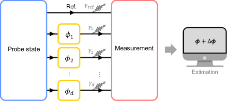
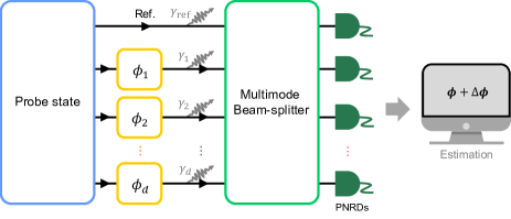
Let us consider a scheme for simultaneously estimating unknown phases in the presence of photon loss as shown in Fig. 1. We assume that the mode 0 is used as a reference upon which the phases of all the other modes are defined. For the multiple-phase estimation, we employ a ()-mode NOON state probe written by
| (1) |
where is the photon creation operator in the mode and with and is the weight of the mode . This probe state undergoes individual phase shifts described by a unitary operator . For practical relevance, we take into account photon loss that could occur in the transmission channels or inefficient detectors. The photon loss can be modeled by a fictitious beam-splitter represented by the mode transformation p.kok with photon loss rate , where is a virtual vacuum input mode for describing environment. It can be shown, by the Kraus representation of photon loss, that photon losses occurring before and after the phase shifters are equivalent. This allows to consider only the photon loss taking place onto the phase-encoded probe state before measurement. The phase-encoded ()-mode NOON state is thus transformed to the output state
| (2) |
where is a photon loss channel in the mode m.grassl . If is zero, then the quantum channel becomes an identity channel. Finally, the estimation of unknown phases is made based on the measurement results obtained by a measurement performed onto the output state of Eq. (2). We also consider an estimation scheme with classical light to examine a quantum advantage of the proposed scheme through quantum parameter estimation theory that is introduced below. As a classical benchmark, we consider the scheme that employs a ()-mode coherent state described by with (, ) under the same environment, leading to the output state followed by measurement and estimation.
II.2 Estimation precision
Denoting as an estimation uncertainty of the unknown phase , the total uncertainty of simultaneous estimation of phases can be defined as the sum of individual uncertainties, i.e., . When an unbiased estimator is used, the total uncertainty is lower-bounded by p.c.humphreys ; j.urrehman ; j.liu2
| (3) |
where is the number of measurement being repeated, is the Fisher information matrix (FIM), and is the quantum Fisher information matrix (QFIM). Here, an FIM element is defined as
| (4) |
with the conditional probability to obtain a measurement outcome conditioned on . QFIM is defined as j.liu2
| (5) |
where denotes the anti-commutation and is a symmetric logarithmic derivative operator with respect to an unknown phase . In Eq. (3), and are called the Cramer-Rao bound (CRB) and the quantum Cramer-Rao bound (QCRB) (per a single measurement try), respectively. Note that the CRB is a lower bound of the total uncertainty determined for a given probe state and a chosen measurement scheme, whereas the QCRB is a further lower bound that would be obtained when an optimal measurement is employed for a given probe state. That is, the CRB becomes the QCRB if a chosen measurement scheme is optimal. However, we need an entanglement-based measurement to attain the QCRB in general, which is experimentally challenging to implement s.hong ; j.urrehman . Thus, it is necessary to consider the CRB provided by a measurement experimentally configurable by linear optics. We also note that the CRB is asymptotically attained by using maximum likelihood estimator when l.pezze ; c.w.helstrom .
III Quantum advantage in terms of the QCRB
III.1 Minimum QCRB of multi-mode NOON states
To evaluate the QCRB, we first derive the output state defined in Eq. (2) for an arbitrary photon number and phases , as
| (6) |
Here, is a non-negative density matrix (see Appendix A) diagonalized in the Fock state basis up to , and is a lossy multi-mode NOON state in the -photon manifold written as
| (7) |
with a normalization constant . One can analytically find the minimum QCRB over all the weighted multi-mode NOON states taking the form of Eq. (1) as
| (8) |
and the optimal weights as
| (9) |
with coefficients (see Appendix B for the details). The minimum QCRB written in Eq. (III.1) successfully encapsulates the previous results in Refs. s.hong ; s.hong2 ; j.urrehman as lossless case. The difference between and () arises because the reference phase is assumed to be known beforehand but the other phases are unknown. We prove that the QCRB of the multi-mode NOON states is attainable (see Appendix C). Thus, the QCRB of the multi-mode NOON states is understood as the minimum estimation uncertainty over all possible measurements.
For the SQL, the minimum QCRB over all multi-mode coherent states can also be found (see Appendix D for the details) and written as
| (10) |
and the optimal weights are
| (11) |
When the photon loss rates are all equal to except the reference mode , the QCRB of Eq. (III.1) is rewritten as
| (12) |
which reduces to
| (13) |
when . For the latter case, the optimal weights are given as
| (14) |
and interestingly these recover the particular multi-mode NOON state proposed by Humphreys’ et al. in Ref. p.c.humphreys . This implies that Humphreys’ NOON states are optimal only when , including the lossless case. On the other hand, the SQL of Eq. (10) is rewritten as
| (15) |
when , and
| (16) |
when all for which the optimal weights take the same form as Eq. (14). A more detailed discussion about these findings is provided below.
III.2 Quantum advantage from two-photon NOON states
Let us here investigate a quantum advantage of the proposed scheme using the multi-mode NOON states in comparison with the SQL under the same lossy environment. The environment that can be characterized in terms of the reference mode and the other modes , which is inspired by the distinct roles that appear through Eq. (III.1) to Eq. (10). To quantify a quantum advantage, we define the ratio of the QCRB for the considered scheme under study to that for the optimized multi-mode coherent states, written as
| (17) |
A positive value of means that a methological performance of the considered scheme surpasses the SQL. In a specific case that , can reduce to
| (18) |
Here, note that a quantum advantage is independent of the mode number and diminishes as becomes larger. On the other hand, the role of the mode number is significant when . It can be easily shown by using Eqs. (III.1) and (15) that, in the case of , the quantum advantage quantified by Eq. (17) is improved by increasing the mode number . Moreover, when a multi-mode NOON state has sufficiently large , the quantum advantage in Eq. (17) converges to as written in Eq. (18), which is independent of the photon loss rate of the reference mode. It is interesting that, for , the quantum advantage of the proposed scheme is irrelevant to the photon loss rate in a reference mode.
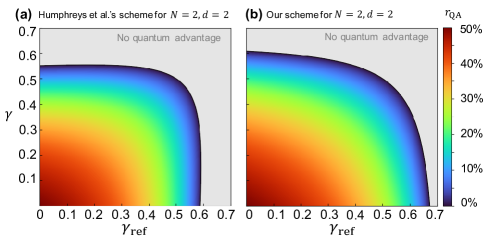
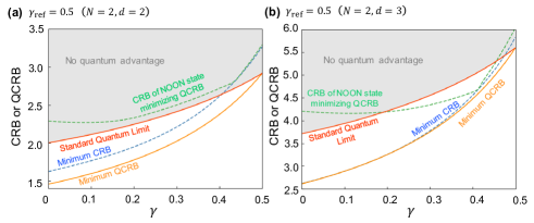
Figure 2 illustrates the regions of photon loss rates where a quantum advantage is achieved for the scheme proposed in Ref. p.c.humphreys (see Fig. 2(a)) and for the scheme we propose with optimal multi-mode NOON states (see Fig. 2(b)) when . It is evident that the colored area of Fig. 2(b) is larger than that of Fig. 2(a), which implies that a multiple-phase estimation scheme proposed in this work is more robust to the photon loss than the scheme proposed in Ref. p.c.humphreys . Also note that the proposed scheme is slightly more robust against the photon loss in the reference mode than that of the other modes.
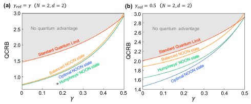
To look into more detailed behaviors, we take two specific values of from Fig. 2(b), and compare different cases including the case using balanced NOON states (i.e., ). In Fig. 3(a), we show that when , our scheme is equivalent to the scheme proposed in Ref. p.c.humphreys , already pointed out in Eq. (14), and the balanced NOON states are also nearly optimal due to equal losses. It can be shown that the equivalence holds for any and , but the near-optimality of the balanced NOON states is degraded with increasing . Interestingly, on the other hand, our scheme becomes significantly advantageous when , which is clearly shown in Fig. 3(b) for the case of that precision difference between these two schemes is well-visible. It reveals that our scheme is better than the scheme in Ref. p.c.humphreys and the balanced NOON states are far from being optimal due to unequal losses. Also note that our scheme can outperform the SQL in the lossy environment, which can be observed in Fig. 3.
III.3 Quantum advantage from -mode -photon NOON states
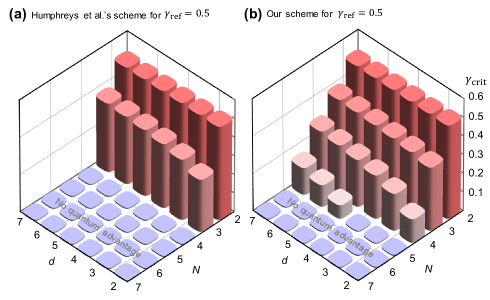
Here, we examine if a quantum advantage is still achievable by -mode -photon NOON states with and how large it is. For the purpose, we define the critical photon loss rate such that a quantum advantage is observed when for where . That is, indicates a robustness of the scheme under study. Figures 4(a) and (b) present for the scheme proposed in Ref. p.c.humphreys and for our scheme, respectively, when as an example that the photon loss of the reference mode is larger than that of the other modes. It is clearly shown that the scheme proposed in this work is more robust against photon loss than Humphreys et al.’s scheme proposed in Ref. p.c.humphreys . Interestingly, the proposed scheme becomes more robust as the number of phases or modes increase. This means that our scheme is useful when the number of phases to be estimated is many, and offers robust multiple-phase estimation schemes even when .
IV Quantum advantage in terms of the CRB
Until the previous section, we have demonstrated that the QCRB of an optimal multi-mode NOON state can surpass the SQL. Exploiting the argument written in Appendix A together with Ref. l.pezze , it is easy to show that a measurement achieving the QCRB has an entanglement-based projection . However, it is known that such the measurement is experimentally challenging to implement in general s.hong2 ; j.urrehman . Thus, for experimental feasibility, we need to verify whether an estimation scheme using a measurement with a linear optical structure can provides the SQL.
We consider a measurement scheme illustrated as Fig. 5 that employs PNRDs with a multi-mode beam-splitter being optimized in the multiple-phase estimation scheme using multi-mode NOON states, and investigate whether the associated CRB evaluated in Appendix E can surpass the SQL and how close it is to be the QCRB of Eq. (III.1). For the optimization over all multi-mode beam-splitters, we exploit Clement’s configuration w.r.clements to represent a general multi-mode beam-splitter as a -mode transformation
| (19) |
Here, is a diagonal unitary matrix and is a block unitary matrix composed of a -dimensional identity matrix and 2 dimensional unitary matrix with real parameters and , which is implemented by a beam-splitter and a phase shifter. Note that consists of redundant phases disappeared from the CRB. In other words, the optimization over all possible multi-mode beam-splitters is equivalent to that over all the real parameters in Eq. (19).
Now, we use the configuration introduced in Eq. (19) for the optimal multi-mode beam-splitter and evaluate the two cases: (i) we optimize the multi-mode beam-splitter for the multi-mode NOON states having minimized the QCRB of Eq. (III.1), and (ii) we optimize simultaneously the multi-mode beam-splitter and the NOON state to minimize the CRB of Eq. (4). The results are shown in Fig. 6 for and when . It is clear that the considered measurement scheme provides mostly inferior performance when applied to the NOON states that have been optimized with respect to the QCRB. However, when both the multi-mode beam-splitter and the NOON states are simultaneously optimized to minimize the CRB, their precision becomes significantly improved and even nearly optimal with respect to the minimum QCRB. Experimental structure of optimal multi-mode beam-splitter depends on the number of modes . The minimum CRB of Fig. 6(a) is attained by a multi-mode beam-splitter with unbalanced ratio, but that of Fig. 6(b) is exhibited from a balanced one.
V Conclusion
We have proposed and studied an optimal scheme of multiple-phase estimation using the weighted multi-mode NOON states under a lossy environment. We have shown that the proposed scheme surpasses the SQL even in the presence of loss, and is more robust to loss than the scheme proposed in Ref. p.c.humphreys that employs only a particular type of multi-mode NOON state. These behaviors persist when the numbers of modes and photons increase, and especially a quantum advantage even increases with the number of modes when the reference mode is lossier than the signal modes carrying the multi-mode NOON states. When the proposed scheme is equipped with a measurement setting configurable by using a multi-mode beam-splitter and PNRDs, a quantum advantage is still achieved although sub-optimal, which provides a practical means in multiple-phase estimation under a lossy environment. We believe the results obtained and the methodology used in this work will motivate various relevant studies in robust quantum metrology under lossy and noisy environments.
An interesting future study would be to apply our methodology to mitigate other types of noises, e.g., the phase-diffusion m.t.dimario , or to estimate other types of multiple parameters of interest, e.g., absorption parameters a.karsa . One may also investigate if similar advantage and robustness can be obtained by employing other strategies such as reference configurations a.z.goldberg or post-selection drm . Another application of this work can be made to estimate a linear function of multiple parameters such as distributed quantum sensing s.-r.zhao ; x.guo ; j.liu3 ; d.-h.kim .
Appendix A. Phase-encoded multi-mode NOON states under photon loss
Here we derive the explicit form of a phase-encoded multi-mode NOON state in Eq. (6) exposed to photon loss. We first note that a quantum channel is described by
| (20) |
with the vacuum state in the environment mode and unitary operator with respect to a mode transformation s.m.barnett , where is the partial trace over the -th environment system. From Eq. (20), It is straightforward to derive three terms , , and as
| (21) |
Substituting the above terms in Eq. (2), the output state is derived as
| (22) |
Appendix B. Evaluation of the minimum QCRB
Here we analytically evaluate the minimum QCRB of -mode NOON states. The non-negative operator in Eq. (22) is diagonalized by vectors of the Fock basis whose photon number is strictly less than . Meanwhile, in Eq. (22) is a linear combination of the Fock basis vectors with photon number equal to . Thus, the support of in Eq. (22) is orthogonal to , and is in the spectral decomposition with the eigenvectors together with . We can employ the theoretical framework written in Ref. j.liu2 to derive components of the QFIM
| (23) |
By using the Sherman-Morrison formula sherman-morrison , the QCRB is evaluated as
| (24) |
which is the convex function of . Since a feasible set of is convex, a global minimum is at the point where gradient of the QCRB in Eq. (24) is vanished s.boyd . Hence, the minimum QCRB is evaluated as Eq. (10) by the optimal weights in Eq. (III.1).
Appendix C. Attainability of the QCRB
It was shown that the necessary and sufficient condition that the QCRB of a quantum state is attained by a measurement is j.liu2
| (25) |
where and are symmetric logarithm derivative operators. By using the above proposition, we show that there is a measurement attaining the QCRB in Eq. (24). From the output state described by Eq. (22), the trace of the left hand side in Eq. (25) is written as linear combination of and with . First, since in Eq. (22) is a multi-mode NOON state, there are symmetric logarithm derivative operators and such that p.c.humphreys . Second, as we consider and of the multi-mode NOON state , their supports are orthogonal to as . Thus, also become zero. Finally, the symmetric logarithm derivative operators satisfy the equality in Eq. (25), which leads us to understand the attainability of the QCRB.
Appendix D. Evaluation of the SQL
Here, we evaluate the SQL quantified by the QCRB of multi-mode coherent states. If the mean photon number of an initial coherent states with is not sufficiently large, then the coherent state in the reference mode is not understood as strong. Thus, it is reasonable to describe a probe state as a phase-averaged multi-mode coherent state a.z.goldberg ; m.jarzyna :
| (26) |
with . Of course, the above probe state encapsulates the case of the strong reference beam when is sufficiently large and is much larger than any with m.jarzyna . Photon loss channels transform the above phase-averaged multi-mode coherent state to
| (27) |
Finally, the QCRB of the above noisy state is analytically evaluated as a.z.goldberg
| (28) |
Thus, the minimum value of the QCRB over all satisfying the relation is straightforwardly evaluated as Eq. (10).
Appendix E. Measurement probabilities for the CRB
For evaluating the CRB, we first derive the FIM in Eq. (4) by deriving the measurement probabilities . Let us start from expressing the measurement probability as
| (29) |
where is a multi-mode Fock basis vector with respect to measurement outcomes , and is a unitary operator of a multi-mode beam-splitter. By representing the unitary transformation with as a scattering matrix , the above measurement probability is derived as
| (30) |
We note that the second term of is independent of the phases . Thus, the CRB is only determined by the first term of Eq. (30) by the definition in Eq. (4).
Acknowledgement
This work was partly supported by National Research Foundation of Korea (NRF) grant funded by the Korea government (MSIT) (2022M3K4A1097123), Institute for Information & communications Technology Planning & Evaluation (IITP) grant funded by the Korea government (MSIT) (2020-0-00947, RS-2023-00222863), and the KIST research program (2E32941).
References
- (1) E. Polino et. al., Photonic quantum metrology, AVS Quantum Sci. 2, 024703 (2020).
- (2) M. Szczykulska, T. Baumgratz, and A. Datta, Multi-parameter quantum metrology, Adv. Phys. X 1, pp. 621-639 (2016).
- (3) J. F. Haase et. al., Precision Limits in Quantum Metrology with Open Quantum Systems, Quantum Meas. Quantum. Metrol. 5, pp. 13-39 (2018).
- (4) L. Z. Liu et. al., Distributed quantum phase estimation with entangled photons, Nat. Photon. 15, pp. 137-142 (2021).
- (5) S. R. Zhao et. al., Field Demonstration of Distributed Quantum Sensing without Post-Selection, Phys. Rev. X 11, 031009 (2021).
- (6) E. Polino et. al., Experimental multiphase estimation on a chip, Optica 6, 288-295 (2019).
- (7) Y. Xia et. al., Demonstration of a reconfigurable entangled radio-frequency photonic sensor network, Phys. Rev. Lett. 124, 150502 (2020).
- (8) R. Schnabel, Squeezed states of light and their applications in laser interferometers, Phys. Rep. 684, pp. 1-51 (2017).
- (9) B. J. Lawrie et. al., Quantum sensing with squeezed light, ACS Photon. 6, pp. 1307-1318 (2019).
- (10) X. Guo et. al., Distributed quantum sensing in a continuous-variable entangled network, Nat. Phys. 16 pp. 281-284 (2020).
- (11) M. Gessner, A. Smerzi, and L. Pezze, Multiparameter squeezing for optimal quantum enhancements in sensor networks, Nat. Comm. 11, 3817 (2020).
- (12) C. Oh, L. Jiang, and C. Lee, Distributed quantum phase sensing for arbitrary positive and negative weights, Phys. Rev. Res. 4, 023164 (2022).
- (13) S.-L. Park, C. Noh, and C. Lee, Quantum loss sensing with two-mode squeezed vacuum state under noisy and lossy environment, Sci. Rep. 13 5936 (2023).
- (14) J. Joo, W. J. Munro, and T. P. Spiller, Quantum Metrology with Entangled Coherent States, Phys. Rev. Lett. 107, 083601 (2011).
- (15) J. Liu et. al., Quantum multiparameter metrology with generalized entangled coherent state, J. Phys. A: Math. Theor. 49, 115303 (2016).
- (16) S.-Y. Lee, Y.-S. Ihn, and Z. Kim, Optimal entangled coherent states in lossy quantum enhanced metrology, Phys. Rev. A 101, 012332 (2020).
- (17) Z. Su et. al., Multiphoton interference in quantum Fourier transform circuits and applicatons to quantum metrology, Phys. Rev. Lett. 119, 080502 (2017).
- (18) M. A. Ciampini et. al., Quntum-enhanced multiparameter estimation in multiarm interferometers, Sci. Rep. 6, 28881 (2016).
- (19) G. Y. Xiang, et. al., Entanglement-enhanced measurement of a completely unknown optical phase, Nat. Photon. 5, pp. 43-47 (2011).
- (20) P. C. Humphreys et. al., Quantum enhanced multiple-phase estimation, Phys. Rev. Lett. 111 070403 (2013).
- (21) L. Zhang and K. W. C. Chan, Quantum multiparameter estimation with generalized balanced multimode NOON-like states, Phys. Rev. A 95, 032321 (2017).
- (22) L. Zhang and K. W. C. Chan, Scalable generation of multi-mode NOON states for quantum multiple-phase estimation, Sci. Rep. 8, 11440 (2018).
- (23) S. Hong et. al., Quantum enhanced multiple-phase estimation with multi-mode NOON states, Nat. Comm. 12, 5211 (2021).
- (24) S. Hong et. al., Practical Sensitivity Bound for Multiple Phase Estimation with Multi-Mode NOON States, Las. Photon. Rev. 16, 2100682 (2022).
- (25) J. ur Rehman et. al., Optimal strategy for multiple-phase estimation under practical measurement with multimode NOON states, Phys. Rev. A 106, 032612 (2022).
- (26) R. Demkowicz-Dobrzanski, J. Kolodynski, and M. Guta, The elusive Heisenberg limit in quantum-enhanced metrology, Nat. Comm. 10, 1038 (2012).
- (27) U. Doner et. al., Optimal Quantum Phase Estimation Phys. Rev. Lett. 102, 040403 (2009).
- (28) R. Demkowicz-Dobrzanski et. al., Quantum phase estimation with lossy interferometers, Phys. Rev. A 80, 013825 (2009).
- (29) J. Kolodynski and R. Demkowicz-Dobrzanski, Phase estimation without a priori phase knowledge in the precense of loss, Phys. Rev. A 82, 053804 (2010).
- (30) M. Kacprowicz et. al., Experimental quantum-enhanced estimation of a lossy phase shift, Nat. Photon. 4, pp. 357-360 (2010).
- (31) J.-D. Yue, Y.-R. Zhang, and H. Fan, Quantum-enhanced metrology for multiple phase estimation with noise, Sci. Rep. 4, 5933 (2014).
- (32) S. L. Barunstein and C. M. Caves, Statistical distance and the geometry of quantum states, Phys. Rev. Lett. 72, 3439 (1994).
- (33) S. L. Barunstein, C. M. Caves, and G. J. Milburn, Generalized Uncertainty Relations: Theory, Examples, and Lorents Invariances, Ann. Phys. 247, pp. 135-193 (1996).
- (34) J. Liu et. al., Quantum Fisher information matrix and multiparameter estimation, J. Phys. A: Math. Theor. 53, 023001 (2020).
- (35) P. Kok and B. W. Lovett, Introduction to Optical Quantum Information Processing (Cambridge University Press, 2010).
- (36) M. Grassl et. al., Quantum Error-Correcting Codes for Qudit Amplitude Damping, IEEE Trans. Inf. Theor. 64, pp. 4674-4685 (2018).
- (37) L. Pezze et. al., Optimal Measurements for Simultaneous Quantum Estimation of Multiple Phases, Phys. Rev. Lett. 119, 130504 (2017).
- (38) C. W. Helstrom, Minimum mean-squared error of estimates in quantum statistics, Phys. Lett. A 25, 101 (1967); Quantum Detection and Estimation Theory (Academic Press, 1976).
- (39) R. J. Glauber, Coherent and Incoherent States of the Radiation Field, Phys. Rev. 131, 2766 (1963).
- (40) A. Z. Goldberg, et. al., Multiphase estimation without a reference mode, Phys. Rev. A 102, 022230 (2020).
- (41) S. Zhou, C.-L. Zou, and L. Jiang, Saturating the quantum Cramér–Rao bound using LOCC, Quant. Sci. Technol. 5, 025005 (2020).
- (42) K. Matsumoto, A new approach to the Cramer-Rao-type bound of the pure-state model, J. Phys. A: Math. Gen. 35, 3111 (2002).
- (43) L. E. Blumenson, A Derivation of n-Dimensional Spherical Coordinates, The American Mathematical Monthly 67, pp. 63-66 (1960).
- (44) W. R. Clements et. al., Optimal design for universal multiport interferometers, Optica 3, pp. 1460-1465 (2016).
- (45) M. T. DiMario et. al., Optimized communication strategies with binary coherent states over phase noise channels, NPJ Quant. Inf. 5, 65 (2019).
- (46) A .Karsa, R. Nair, A. Chia, K.-G. Lee, and C. Lee, Optimal quantum metrology of two-photon absorption, arXiv:2311.12555 (2023).
- (47) D. R. M. Arvidsson-Shukur et. al., Quantum advantage in postselected metrology, Nat. Comm. 11, 3775 (2020).
- (48) L.-Z. Liu et. al., Distributed quantum phase estimation with entangled photons, Nat. Photon. 15, pp. 137–142 (2021).
- (49) D.-H. Kim et. al., Distributed quantum sensing of multiple phases with fewer photons Nat. Comm. 15, 266 (2024).
- (50) S. Boyd and L. Vandenberghe, Convex Optimization Problem (Cambridge University Press, 2009).
- (51) S. M. Barnett and P. M. Radmore Methods in Theoretical Quantum Optics (Oxford University Press, 2002).
- (52) M. Jarzyna and R. Demkowicz-Dobrzański, Quantum interferometry with and without an external phase reference Phys. Rev. A 85, 011801(R) (2012).
- (53) J. Sherman and W. J. Morrison, Adjustment of an Inverse Matrix Corresponding to a Change in One Element of a Given Matrix Ann. Math. Stat. 21, pp. 124-127 (1950).