First Observation of the Complete Rotation Period of the Ultra-Slowly Rotating Magnetic O Star HD 54879

Abstract

HD 54879 is the most recently discovered magnetic O-type star. Previous studies ruled out a rotation period shorter than 7 years, implying that HD 54879 is the second most slowly-rotating known magnetic O-type star. We report new high-resolution spectropolarimetric measurements of HD 54879, which confirm that a full stellar rotation cycle has been observed, and derive a rotation period of $\mathrm{P}=2562^{+63}_{-58}$ d (about 7.02 yr). The radial velocity of HD 54879 has been stable over the last decade of observations. We explore equivalent widths and longitudinal magnetic fields calculated from lines of different elements, and conclude the atmosphere of HD 54879 is likely chemically homogeneous, with no strong evidence for chemical stratification or lateral abundance nonuniformities. We present the first detailed magnetic map of the star, with an average surface magnetic field strength of 2954 G, and a strength for the dipole component of 3939 G. There is a significant amount of magnetic energy in the quadrupole components of the field (23 %). Thus, we find HD 54879 has a strong magnetic field with a significantly complex topology.

1 Introduction

The large-scale spectropolarimetric surveys of OB stars conducted over the last two decades (e.g., BoB, MiMeS; Morel et al., 2015; Wade et al., 2016) have detected surface magnetic fields in around $\sim$7% of massive OB stars. These fields typically have dipolar topologies, are globally organized, and are strong ($\sim$1 kG) and stable over timescales of decades (Petit et al., 2013; Grunhut et al., 2017; Shultz et al., 2018, 2019). Magnetic O-type stars are rare; thus, the detailed characterization of their field strengths and geometries is an important contribution to a developing understanding of this unique population.

The surface magnetic fields of OB stars significantly impact the star’s long-term evolution (see, e.g., Keszthelyi 2023 for a recent review). Petit et al. (2017) and Georgy et al. (2017) used the mass-loss quenching formalism of ud-Doula & Owocki (2002) to demonstrate that magnetic massive stars retain much more mass during their main sequence evolution than inferred from non-magnetic evolutionary models. Similarly, the effect of magnetic braking, following ud-Doula et al. (2009), has been incorporated into massive star evolutionary models, showing a rapid decline of the surface rotation (Meynet et al., 2011; Keszthelyi et al., 2019, 2020, 2021, 2022). An extreme example of magnetic braking is found in the O4-7.5f?p star HD 108, which has the longest rotation period of all known O stars (54 yrs; Nazé et al., 2001; Shultz & Wade, 2017; Rauw et al., 2023). HD 108 thus stands in stark contrast to the other 12 well-established magnetic O-type stars in our galaxy whose rotation periods are typically on the order of several days to months (Petit et al., 2013; Grunhut et al., 2017).

The topic of this study, HD 54879, is a main sequence O9.7V star (Sota et al., 2011) that is distinguished by its strong magnetic field and very slow rotation. Spectropolarimetric measurements of the star were first obtained as a part of the B-fields in OB stars (BOB) survey (e.g., Morel et al., 2015), with the definite detection of the star’s magnetic field initially announced by Castro et al. (2015) and Fossati et al. (2015). Both papers reported the observed negative extremum of the star’s longitudinal magnetic field ($\langle B_{z}\rangle$) curve to be $\sim$ -600 G, implying a strong surface magnetic field of at least 2 kG. Additional spectropolarimetric monitoring by Wade et al. (2020) and Järvinen et al. (2022) showed a slow increase of the longitudinal field to an observed positive extremum of $\langle B_{z}\rangle\sim$ 74 G, before once again passing through magnetic null.

To date, estimates of the rotation period of HD 54879 have been based on fits to the incomplete monitoring of the longitudinal magnetic field curve. These indicated the rotation period was longer than five years (Wade et al., 2020). The most recent sinusoidal fit reported by Järvinen et al. (2022) suggested a stellar rotation period of 7.2 yr, placing HD 54879 as the second slowest rotator among the known magnetic O star population.

HD 54879’s spectra show clear evidence of strong H$\alpha\;$emission, interpreted by Castro et al. (2015) as likely originating from circumstellar material. Shenar et al. (2017) reported variability in the star’s H$\alpha\;$profiles over both short-term (days) and long-term (months to years) timescales, with the former being attributed to stochastic processes in the stellar wind (e.g., Sundqvist et al., 2012; ud-Doula et al., 2013), and the latter to variability associated with stellar rotation. These conclusions were supported with additional monitoring of the star reported by Hubrig et al. (2020) and Järvinen et al. (2022).

In this paper, we report the most recent spectropolarimetric measurements of HD 54879. The data, described in Section 2, indicate the $\langle B_{z}\rangle$ curve has once again turned over, providing evidence that observations now span one complete rotation cycle. We perform a new magnetic analysis in Section 3, and we provide a refined measurement of the stellar rotation period. We examine the radial velocity and H$\alpha\;$variability of the star, and investigate claims of differences in the strength of the longitudinal magnetic field of the star when the field is measured from lines of individual elements. We also present the first magnetic map of HD 54879. Our findings are discussed in Section 4.

2 Observations

2.1 ESPaDOnS Spectropolarimetry

Three new sets of high-resolution ($R\sim 68,000$) spectropolarimetric sequences of HD 54879 were obtained using the ESPaDOnS echelle spectropolarimeter at the Canada-France-Hawaii Telescope (CFHT) on 2021 February 24, 2022 February 20, and 2023 October 21. A log of these observations is provided in Table 1. The ESPaDOnS instrument covers an approximate wavelength range of 3700-10500 Å across 40 spectral orders. Each spectropolarimetic sequence consists of four subexposures, and yields four Stokes $I$ spectra, one Stokes $V$ spectrum, and two null ($N$) spectra, which were extracted using the methods described by Donati et al. (1997). A detailed description of the reduction and analysis of ESPaDOnS data is provided in Wade et al. (2016). Each subexposure in the 2021 and 2022 measurements had a duration of 867 s; similarly, each of the 2023 subexposures had a duration of 880 s. The peak signal-to-noise ratio per 1.8 km s^-1 pixel near 550 nm of the recently obtained Stokes $V$ spectra ranges between 729 and 830. Thus, the new data are of similar quality to the available archival observations from ESPaDOnS.

2.2 Archival Data Sets

In Table 1 and in our corresponding analysis, we include all available archival spectropolarimetric observations of HD 54879 that were obtained with HARPSpol, mounted on the 3.6 m telescope at the European Southern Observatory’s (ESO) La Silla Observatory (Piskunov et al., 2011); with the Narval spectropolarimeter, mounted on the Bernard Lyot Telescope (TBL) at the Pic du Midi Observatory (Aurière, 2003); and with ESPaDOnS at CFHT. The original reduction and analysis of these data were presented by Castro et al. (2015), Wade et al. (2020) and Järvinen et al. (2022). We have performed a complete reanalysis of the archival data, in conjunction with the new observations, to provide as consistent and homogeneous a set of results as possible. Our extracted longitudinal magnetic field and null profile ($\langle N_{z}\rangle$) values are consistent within uncertainties to the data reported by Wade et al. (2020), and are presented in Table 1.

3 Magnetic and Spectroscopic Analysis

Table 1: Archival and newly obtained (indicated by ^∗ in the Instrument column) spectropolarimetric observations of HD 54879, from HARPSpol (H), ESPaDOnS (E), and Narval (N). The longitudinal magnetic field ($\langle B_{z}\rangle$) and null spectrum ($\langle N_{z}\rangle$) are calculated using profiles computed with a least-squares deconvolution method, with an integration range of $+5$ to $+50$ km sec^-1. The phase $\phi$ is calculated using the ephemeris and 2562 d period described in Equation 1. The peak S/N is around 550 nm for all spectra.

HJD	$\langle B_{z}\rangle$	$\langle N_{z}\rangle$	RV	Peak	$\phi$	Inst
- 2455000	(G)	(G)	(km s-1)	S/N
1770.4993	-631$\pm$12	-17$\pm$11	27.77$\pm$0.03	270	0.00	H
1971.0658	-561$\pm$12	-1$\pm$10	27.64$\pm$0.06	795	0.08	E
1971.1066	-568$\pm$12	14$\pm$10	27.61$\pm$0.06	810	0.08	E
2030.5195	-542$\pm$19	-4$\pm$18	27.74$\pm$0.06	459	0.10	N
2032.5133	-544$\pm$18	-1$\pm$17	27.69$\pm$0.06	479	0.10	N
2033.5159	-531$\pm$19	1$\pm$17	27.76$\pm$0.06	480	0.10	N
2092.5485	-504$\pm$12	-24$\pm$12	27.76$\pm$0.03	233	0.12	H
2095.5057	-509$\pm$19	15$\pm$19	27.76$\pm$0.03	156	0.13	H
2310.6113	-491$\pm$37	31$\pm$36	27.61$\pm$0.06	246	0.21	N
2338.6680	-445$\pm$38	-10$\pm$37	27.60$\pm$0.06	229	0.22	N
2357.6202	-459$\pm$37	2$\pm$36	27.67$\pm$0.06	228	0.23	N
2374.5860	-444$\pm$33	16$\pm$33	27.69$\pm$0.06	255	0.23	N
2409.5524	-492$\pm$36	-19$\pm$35	27.68$\pm$0.06	260	0.25	N
2439.4167	-538$\pm$49	-72$\pm$49	27.56$\pm$0.06	191	0.26	N
2736.9835	-410$\pm$16	-3$\pm$15	27.47$\pm$0.06	525	0.38	E
2758.8779	-409$\pm$17	6$\pm$16	27.46$\pm$0.06	518	0.38	E
2775.9878	-409$\pm$15	-17$\pm$14	27.49$\pm$0.06	587	0.39	E
2880.7390	-348$\pm$17	12$\pm$17	27.61$\pm$0.06	553	0.43	E
3008.1272	-224$\pm$12	-7$\pm$12	27.68$\pm$0.06	644	0.48	E
3066.0351	-182$\pm$12	-5$\pm$12	27.55$\pm$0.06	649	0.50	E
3128.9253	-125$\pm$14	8$\pm$14	27.38$\pm$0.06	514	0.53	E
3557.8753	75$\pm$15	-2$\pm$15	27.58$\pm$0.06	658	0.70	E
3744.1304	-24$\pm$13	1$\pm$12	27.70$\pm$0.06	678	0.77	E
4269.8770	-637$\pm$14	2$\pm$12	27.54$\pm$0.06	729	0.97	E∗
4630.8714	-500$\pm$11	-3$\pm$9	27.53$\pm$0.06	830	1.12	E∗
5239.0541	-427$\pm$11	0$\pm$10	27.57$\pm$0.05	779	1.35	E∗

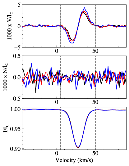
Figure 1: Top to bottom: the Stokes $V$, null, and Stokes $I$ profiles extracted from the three most recent observations of HD 54879, corresponding to Julian dates ($-2455000$) 4269.8770 (blue), 4630.8714 (red), and 5239.0541 (black) from Table 1. The integration range of $+5$ to $+50$ km sec^-1 is indicated by the gray dashed lines in each panel. The $V$ spectra deviate significantly from zero while the Null spectrum does not, indicating the detection of the star’s magnetic field in these data.

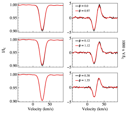
Figure 2: Stokes $I$ (left column) and Stokes $V$ (right column) profiles of the most recent spectropolarimetric measurements of HD 54879 (red) compared to archival data of the star at approximately the same rotation phase $\phi$ (black), but one cycle previous to the new data. The profiles are consistent with each other.

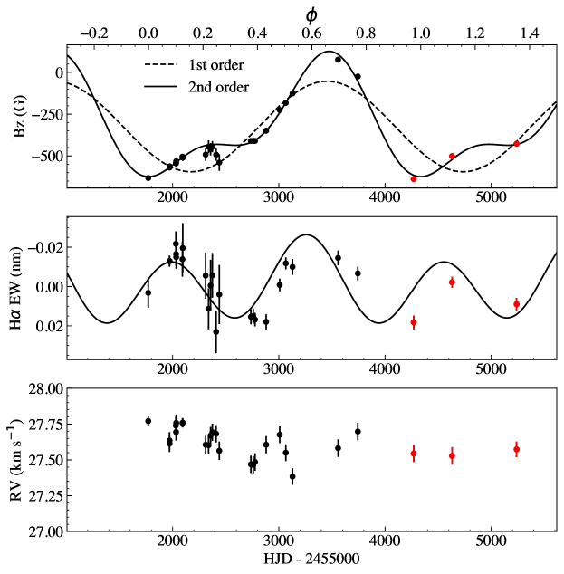
Figure 3: Upper panel: The phased time series of $\langle B_{z}\rangle$ measurements. The lower x-axis references the date of the observations, with the archival data sets in black dots, and the data from the 2021-2023 observing epochs in red. The timestamps are phased according to an ephemeris with $P=2562$ d and $t_{0}=2456774$ (HJD), reported along the top axis. The dashed and solid black lines show the 1st and 2nd order fits to the $\langle B_{z}\rangle$ data, respectively. Middle panel: The phased time series of H$\alpha$ equivalent width measurements, with colors as above. Overplotted is the best fit using a 2-component harmonic function with the same period and ephemeris as the upper panel. Lower panel: Radial velocity measurements as a function of heliocentric Julian Date, with colors as above.

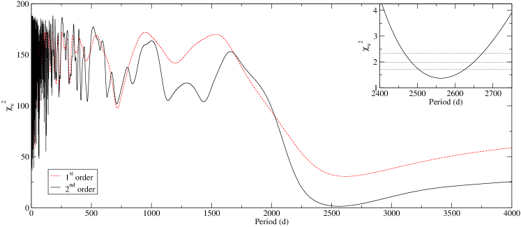
Figure 4: Periodograms from fitting the $\langle B_{z}\rangle$ data using 1st (red dashed line) or 2nd (black line) order Fourier series. In the inset frame, dotted lines represent $\chi_{\nu}^{2}$ contours for 1, 2, and 3$\sigma$ confidence levels, about the best period for the 2nd order Fourier series fit.

3.1 Longitudinal magnetic field

The first step of the spectroscopic analysis was to normalize the spectra to their continuum. This was done by fitting low degree polynomials through carefully selected continuum points, and spectral orders were normalized individually. We started from unnormalized extracted spectra for both the new and archival observations, to provide a consistent normalization for all data.

We used Least-Squares Deconvolution (LSD; Donati et al. 1997) to calculate pseudo-average line profiles for the intensity, Stokes $V$ and null spectra. This technique effectively boosts the signal-to-noise ratio of the Zeeman signatures present in the Stokes $V$ profiles, to enable the detection of stellar magnetic fields. Here we use a new open source implementation of the LSD algorithm. This follows the description of Kochukhov et al. (2010), and provides results fully consistent with their iLSD code. We used the custom line mask of Wade et al. (2020), based on data from the Vienna Atomic Line Database (VALD3; Piskunov et al. 1995; Ryabchikova et al. 1997, 2015; Kupka et al. 1999, 2000). This mask includes only metal lines, and excludes He lines. The observed He lines do not meet the self-similarity hypothesis of LSD, and display a variety of shapes due to varying amounts of Stark broadening, thus they were rejected. We verified that this mask is well optimized for the spectral lines present in observations from all three instruments, and used it consistently for all the spectra. We used a normalizing wavelength of 500 nm, effective Landé factor of 1.2, and depth of 0.1 for the LSD calculation. Every LSD Stokes $V$ profile produced a definite detection, with the corresponding null profiles producing non-detections.

The Stokes $I$, $V$, and null LSD profiles from the most recently obtained ESPaDOnS data are shown in Figure 1. The Stokes $V$ profiles show typical Zeeman signatures with a large amplitude (corresponding to the $\langle B_{z}\rangle$ measurements in Table 1). In Figure 2, we compare these profiles to archival observations obtained at similar rotation phases (using the ephemeris found below). The profiles have nearly identical morphologies, amplitudes, and polarities, supporting the stability of the magnetic field and our derived period.

The longitudinal magnetic field was measured from the LSD profiles using a first moment technique (e.g., Wade et al., 2000) with an integration range of $+5$ to $+50$ km s^-1, and the normalizing wavelength and Landé factor of the LSD profiles. This is consistent with the procedure from Wade et al. (2020). We report the $\langle B_{z}\rangle$ and $\langle N_{z}\rangle$ (the $\langle B_{z}\rangle$ calculation performed on the null profile) for all observations in Table 1. Measurements from the three new polarimetric sequences indicate a dramatic decrease in the magnitude of the longitudinal magnetic field (from $-24$ G to $-637$ G), with a subsequent, smaller increase (to $-500$ G and $-427$ G). These values are close to the initial measurements of the longitudinal magnetic field strength from Castro et al. (2015) and Wade et al. (2020), strongly suggesting the magnetic field has now been observed over one complete rotational cycle.

Generally, the $\langle B_{z}\rangle$ and $\langle N_{z}\rangle$ values we find here are in good agreement with Wade et al. (2020). Comparing results for the same observations, they mostly differ by $<1\sigma$ of the joint error and always by $<2\sigma$. Our results are in reasonable agreement with Castro et al. (2015), who report $\langle B_{z}\rangle$ for the first HARPSpol observation calculated with three different methods. Compared with their ‘Bonn’ LSD analysis (the most similar to our procedure) our result is stronger by -39 G with a joint error bar of 14 G, which is an acceptable agreement given differences in the line masks used. Our results consistently disagree by $>3\sigma$ with the metal line analysis of Hubrig et al. (2020), who reanalyzed the ESPaDOnS data of Wade et al. (2020) but found differing $\langle B_{z}\rangle$ values. Hubrig et al. (2020) present results for two observations obtained on the same night (JD 2456971) with $\langle B_{z}\rangle$ values differing by $\sim 5\sigma$ (81 G), which suggests they substantially underestimated the real uncertainty in their results. Our results disagree with Järvinen et al. (2021) by $>3\sigma$ for about half of the observations we have in common, based on their LSD analysis using all metal lines (their most similar results). Järvinen et al. (2021) similarly disagree with Wade et al. (2020). They partially agree with Hubrig et al. (2020), with 6 of 9 of the measurements in common differing by $<2\sigma$. Järvinen et al. (2021) find large differences in $\langle B_{z}\rangle$ over short periods of time (up to 196 G in 39 days), which are not seen in other studies of the same data (and not seen in some of their alternative line masks). This suggests that there are significant systematic errors or underestimated uncertainties in some of their values.

The longitudinal magnetic field curve of HD 54879, presented in the upper panel of Figure 3, shows significant departures from what is expected from a dipolar topology (see also Section 3.5 below). To date, topologically complex magnetic fields with strong departures from a dipole have only been reported in one other O-type star (NGC 1624-2; David-Uraz et al., 2021; Järvinen et al., 2021), although complex geometries have also been found in a few early B-type stars (e.g. Donati et al., 2006; Kochukhov et al., 2011). In this figure, we also show a first-order sinusoidal fit to the data (dashed line), which would be expected for a purely dipolar field. Also included is a second-order harmonic fit to the data (solid line), which is equivalent to including both dipolar and quadrupolar components.

Since the $\langle B_{z}\rangle$ measurements now cover a full rotation cycle, we can perform a periodogram analaysis. We proceeded by fitting Fourier functions to the data for a grid of fixed periods, and recording the resulting reduced chi-squared ($\chi_{\nu}^{2}$) for each period. For a first order function this is equivalent to a Lomb-Scargle periodogram, except in units of $\chi_{\nu}^{2}$ rather than power, but this approach can be generalized for more complex magnetic fields by using a second or third order Fourier series. Periodograms for both the first and second order Fourier series fits are shown in Figure 4. The first order fit produced a $\chi_{\nu}^{2}$ minimum near our adopted period, but with $\chi_{\nu}^{2}>30$, reflecting a strong departure from a dipolar magnetic field. The second order fit reaches $\chi_{\nu}^{2}=1.37$, reflecting an adequate fit to the observations. Using the second order fit, and placing the negative magnetic extremum at phase zero, we adopt the ephemeris:

$$HJD=2456774+2562^{+63}_{-58}E$$ (1)

Thus the current best fit rotation period is $\mathrm{P}=2562^{+63}_{-58}$ d, or about 7.02 yr.

The departure of the $\langle B_{z}\rangle$ curve from that expected for a pure dipole is highly statistically significant, which indicates a more complex magnetic topology. The success of the second order fit to the $\langle B_{z}\rangle$ curve suggests that there is a strong quadrupolar component to the magnetic field. As noted above, such complex fields have been observed around cooler stars, such as $\tau$ Sco (B0.2V; Donati et al., 2006), $\alpha^{2}$ CVn (B9p; Silvester et al., 2014), and HD 37776 (B2V; Kochukhov et al., 2011), but had not yet been so prominently observed in the $\langle B_{z}\rangle$ curve of an O-type star.

3.2 Radial velocity stability

With the LSD profiles calculated in Sect. 3.1, we calculated precise radial velocities for HD 54879. The LSD calculations used a mask with most available metal lines in the spectra. Radial velocities were determined by fitting a Gaussian to the Stokes $I$ profiles using $\chi^{2}$ minimization, and taking the centeroid. Uncertainties were taken from the square root of the diagonal of the covariance matrix, and thus only incorporate the pixel uncertainties in the LSD Stokes $I$ profiles.

A plot of the radial velocity data as a function of time is in Figure 3 (lower panel), and this reveals no periodicity or significant trends with time. The radial velocities are highly stable within observations from one instrument, and are in good agreement between instruments. The full average is 27.62 km s^-1 with a standard deviation of 0.10 km s^-1. For just the 14 ESPaDOnS observations, the average is 27.56 km s^-1, with a mean uncertainty of 0.06 km s^-1, and standard deviation 0.08 km s^-1. For the 9 Narval observations, the average is 27.67 km s^-1, with mean uncertainty and standard deviation of both 0.06 km s^-1. For the HARPSpol data, the average is 27.76 km s^-1 with a mean uncertainty of 0.03 km s^-1.

We thus conclude that the radial velocity of HD 54879 has been stable to better than 0.1 km s^-1 for the last 9.5 years. This definitively rules out proposals that this is an SB1 binary (e.g. Hubrig et al., 2019), unless the period is very long ($\gg 10$ yr). This stability also argues against most other kinds of metal line variability, such as chemical spots, although we investigate that in more detail below.

3.3 Measuring the magnetic field from lines of individual elements

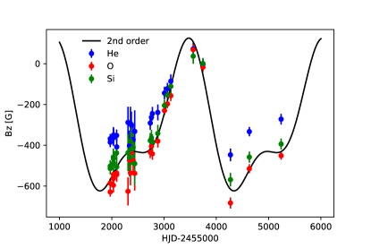
Figure 5: Measurements of the longitudinal magnetic field from LSD profiles of He, O and Si lines. The black curve is the best-fit second-order sine curve from Section 3.

Järvinen et al. (2022) reported in their abstract, “The most intriguing result of our study is the discovery of differences in longitudinal magnetic field strengths measured using different least-squares deconvolution (LSD) masks containing lines belonging to different elements… Since the LSD Stokes $I$ profiles of the studied O, Si, and He line masks remain stable over all observing epochs, we conclude that the detection of different field strengths using lines belonging to these elements is related to the different formation depths, with the He lines formed much higher in the stellar atmosphere compared to the silicon and the oxygen lines, and non-local thermodynamic equilibrium (NLTE) effects.” This sentence may be implying that O, Si, and He have vertically non-uniform abundance distributions, i.e. that they are stratified. However, later in their article the authors state, “Thus, we conclude that the elements O, Si, and He are not uniformly distributed over the stellar surface [our emphasis] of HD 54879, but that the formation of their spectral lines takes place at different atmospheric heights, with He lines formed much higher in the stellar atmosphere compared to the Si and O lines.” This latter sentence appears to imply that O, Si and He have non-uniform lateral distributions, possibly in addition to being vertically stratified.

The different LSD masks associated with each of the elements they analyzed are comprised of different collections of lines of different depths, landé factors, and widths, and certainly correspond to somewhat different measurement systems. Without calibration it is not surprising that the LSD profiles and longitudinal fields extracted using these different masks would be somewhat different. Nevertheless, we carried out an independent analysis of the observations using single-element line masks. We used the iLSD code of Kochukhov et al. (2010) in multi-mask mode. (It is not clear which LSD code Järvinen et al. (2022) employed.) Starting from the line mask of Wade et al. (2020), we created three new line masks containing only O lines, Si lines, and He lines, along with their associated anti-masks (i.e. the original mask excluding the lines of each of those elements). We then extracted LSD profiles for each element, taking into account the blending by other elements using the anti-masks. Finally, we measured the longitudinal magnetic field from each profile. Those measurements are shown in Figure 5.

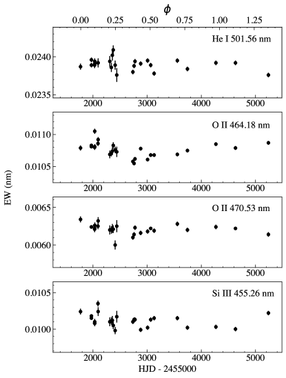
Figure 6: Equivalent widths from individual lines of He, O and Si. No significant variability is evident.

As reported by Järvinen et al. (2022), there are some differences in the amplitudes of the $\langle B_{z}\rangle$ variations for individual elements. However, the various $\langle B_{z}\rangle$ curves have the same essential shapes, i.e. they are not strongly discrepant like those of chemically peculiar B-type stars such as HD  184927 (Yakunin et al., 2015). Moreover, we observe no significant variations of line profiles or equivalent widths (shown in Figure 6) of these elements, either in LSD profiles or individual spectral lines. These lines of evidence all point to small differences in the measurement systems corresponding to the various line masks, leading to small differences in the inferred longitudinal fields. We thus conclude that there is no compelling evidence for chemical stratification or lateral abundance nonuniformities in the atmosphere of HD  54879.

3.4 H$\alpha$ Emission

HD 54879 exhibits atypically strong H$\alpha$ emission for its spectral type (Boyajian et al., 2007; Castro et al., 2015), with variability on both short (days) and long (years) timescales (Shenar et al., 2017). Mass-loss rate estimates derived from this H$\alpha$ emission are comparatively too large (by an order of magnitude; Castro et al., 2015), and so are considered unreliable. Castro et al. (2015) suggested that HD 54879’s H$\alpha$ emission is likely magnetospheric in origin. For a star with a circumstellar magnetosphere, outflowing line-driven stellar winds can become trapped by the magnetic field and are forced to corotate with the star. Typically, in slowly rotating stars, rotation is not fast enough to provide sufficient centrifugal support for the plasma to overcome gravity. The confined wind material will fall back to the stellar surface under the influence of gravity on a dynamical timescale, forming a “Dynamical Magnetosphere” (DM; Sundqvist et al., 2012). In the spectra of stars hosting DMs, H$\alpha$ emission has been observed to have a single broad peak close to line center (e.g., Petit et al., 2013). The multi-peaked H$\alpha$ emission from HD 54879, illustrated in Figure 7, suggests its circumstellar environment is shaped by a complex magnetic field.

To explore the variation of the H$\alpha$ profile and how it relates to the rotation period derived from $\langle B_{z}\rangle$ measurements, we compute equivalent width measurements using the spectra listed in Table 1. First, we refine the normalization that has already been applied to the spectra for the magnetometric analysis by defining continuum regions on either side of the H$\alpha$ line (653.9-654.1 nm blueward, and 658.85-659.05 nm redward), and renormalizing the H$\alpha$ line to a linear fit to those averaged regions. The resulting lines are shown overplotted in Figure 7.

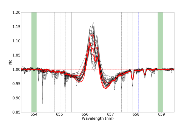
Figure 7: H$\alpha$ line from spectra taken with HARPS, NARVAL and ESPaDOnS (see Table 1). The archival data are plotted as black solid lines, while the new data sets are indicated in red. The continuum region used for local normalization are highlighted with green vertical shading. The other vertical lines correspond to the integration bounds that were tested for the calculation of equivalent widths, i.e. $\pm$400 km s^-1 (solid black), $\pm$500 km s^-1 (dashed black), $\pm$600 km s^-1 (dash-dotted black), $\pm$700 km s^-1 (dotted black), and $\pm$800 km s^-1 (dashed blue). We can see from this figure that HD 54879 exhibits significant H$\alpha$ emission at all rotational phases that were observed.

We then conducted some tests to determine the best integration range over which to compute our equivalent width measurements. We tried integration bounds at $\pm$400, 500, 600, 700, and 800 km s^-1 with respect to the H$\alpha$ line center (accounting for the systemic velocity of 27.62 km s^-1; see Section 3.2). As can be seen in Figure 7, all magnetospheric variability appears to be contained with the bounds at $\pm$400 km s^-1, with larger bounds including undesirable photospheric lines overlapping with the wings of the H$\alpha$ line profile. Equivalent widths computed with these various bounds followed a similar trend from one spectrum to another, with uncertainties increasing with larger bounds. This indicates that indeed, the smallest bounds contain the bulk of the magnetospheric variability, and therefore they were used for the rest of the analysis (even though they do not span the full H$\alpha$ line profile).

Figure 3 (middle panel) shows the clearly coherent variation of the H$\alpha$ equivalent widths with time. The measurements are fit with a second-order harmonic curve (black line) with a period corresponding to that derived from the $\langle B_{z}\rangle$ analysis. Most of the equivalent width variability is consistent with this sinusoidal fit, modulated at the rotation period. However, we also performed an empirical harmonic fit to the H$\alpha\;$data with a partly unconstrained period (it was allowed to vary between 2400 and 2900 d). We found that a 2-component function is significantly preferred over a single sinusoid (with a reduced $\chi^{2}$ of 1.031 rather than 1.977). This method (with the 2-component function) yielded a best-fit period of 2827 d ($\sim$7.75 yr). Both estimates of the rotation period are within the same order of magnitude. Shorter-term variability, as observed by Shenar et al. (2017) and also evidenced in our measurements (see Figure 3), could conceivably cause systematics in the determination of the period using equivalent width measurements, although it appears unlikely to fully explain the discrepancy between the periods derived from both methods. Further investigation, both observationally (more coverage) and theoretically (e.g., modeling H$\alpha$ emission using analytical prescriptions; Owocki et al. 2016) will be needed to resolve this tension. Nevertheless, the H$\alpha$ equivalent width variation supports our overall conclusion that HD 54879 rotates extremely slowly.

3.5 Magnetic Geometry

The strong, complex field of HD 54879, combined with its long rotation period and assumed young age, make it a particularly interesting candidate for Zeeman Doppler Imaging (ZDI; Donati & Brown, 1997; Piskunov & Kochukhov, 2002), a technique used to create a surface map of the star’s magnetic field. To date, only one O-type star has been mapped in detail using ZDI (Plaskett’s star; Grunhut et al., 2022). The typically large macroturbulent broadening of O star spectral lines (and therefore Zeeman signatures) makes ZDI mapping challenging. HD 54879 has a relatively low macroturbulence ($v_{\rm mac}$ $=8\pm 3$ km s^-1, Castro et al. 2015; $v_{\rm mac}$ $<4$ km s^-1, Shenar et al. 2017; $v_{\rm mac}$ $=8$ km s^-1, Holgado et al. 2022), although its slow rotation implies $v\sin i$ is still much less than the macroturbulence. Nevertheless, with the very high S/N and relatively complete rotation phase coverage provided by our observations, the most important large-scale components of the magnetic geometry can be reconstructed with ZDI.

For this analysis we adopted the rotation period ($2562^{+63}_{-58}$ d) and ephemeris from the $\langle B_{z}\rangle$ data. Using the rotation period and a radius one can derive the equatorial rotation velocity ($v_{\rm eq}$). Castro et al. (2015) reported $R=6.7^{+1.0}_{-0.9}~{}R_{\odot}$ based on comparing spectroscopic $T_{\rm eff}$ and $\log g$ with evolutionary tracks from bonnsai. Shenar et al. (2017) reported $R=6.1\pm 1.5~{}R_{\odot}$, based on $T_{\rm eff}$ and luminosity with the Stefan-Boltzmann law. Here we adopted the value of Shenar et al. (2017), although the exact value has very little impact on the ZDI results, giving us $v_{\rm eq}=0.12\pm 0.03$ km s^-1.

3.5.1 Unno-Rachkovsky line model

An initial attempt to fit the Stokes $V$ LSD profiles using ZDI and a line model relying on the weak field approximation (specfically Folsom et al., 2018a) failed. The width of the Stokes $V$ profile varies and is narrower around phases 0.6-0.8, with the peaks closer to line center than most other phases. With $v\sin i$ $\leq 0.12$ km s^-1, a weak field model cannot reproduce this variation in Stokes $V$ width. A model that incorporates Zeeman broadening due to a strong magnetic field is needed.

We used a modified version of the ZDIpy code (Folsom et al., 2018a), that incorporates an Unno-Rachkovsky model for the local line profile. This code is described by Bellotti et al. (2023), and follows the work of Donati et al. (2008) and Morin et al. (2008). The code still uses a spherical harmonic description of the magnetic field (Donati et al., 2006), the maximum entropy fitting routine of Skilling & Bryan (1984), and the entropy formulation of Hobson & Lasenby (1998) calculated from the spherical harmonic coefficients. The Unno-Rachkovsky calculation follows the description in Landi Degl’Innocenti & Landolfi (2004). This is essentially a Milne-Eddington line model extended to solve the polarized radiative transfer equation. Since we are modeling LSD profiles rather than individual lines, we assume a simple triplet Zeeman splitting pattern. Local line opacity and anomalous dispersion profiles are taken to be Voigt and Faraday-Voigt profiles, respectively. Morin et al. (2008) and Bellotti et al. (2023) include filling factors in their line model, but these are not used here (or equivalently $f_{I}=f_{V}=1$).

The model used here allows separate parameters for limb darkening (in continuum brightness), and the slope of the source function in the Milne-Eddington atmosphere ($\beta$ in equation [9.105] of Landi Degl’Innocenti & Landolfi 2004). This decouples the effects of brightness decreasing towards the limb and local line strength decreasing towards the limb. In the calculations, the local line profiles are normalized by the local continuum and then scaled by the local limb darkening. However, the linear approximation of a Milne-Eddington atmosphere implies a linear limb darkening. The local continuum flux is

$$I_{c}=B_{0}(1+\beta\cos\theta)$$ (2)

(see Landi Degl’Innocenti & Landolfi, 2004, equations 9.105-9.112) $B_{0}$ is the surface value of the source function, and $\theta$ is the angle between the line of sight and surface normal. The local continuum flux relative to the flux at disk center is

$$I_{c}/I_{c}^{0}=(1+\beta\cos\theta)/(1+\beta).$$ (3)

A standard linear limb darkening law (e.g. Gray, 2005) is

$$I_{c}/I_{c}^{0}=1-\eta+\eta\cos\theta$$ (4)

for a limb darkening coefficient $\eta$. One can derive $\beta$ directly from $\eta$:

$$\beta=\eta/(1-\eta).$$ (5)

We used this relation to set the slope of the source function to be consistent with the desired continuum limb darkening. This is convenient since tabulations of $\eta$ are available for a wide range of stars.

3.5.2 Optimal model parameters

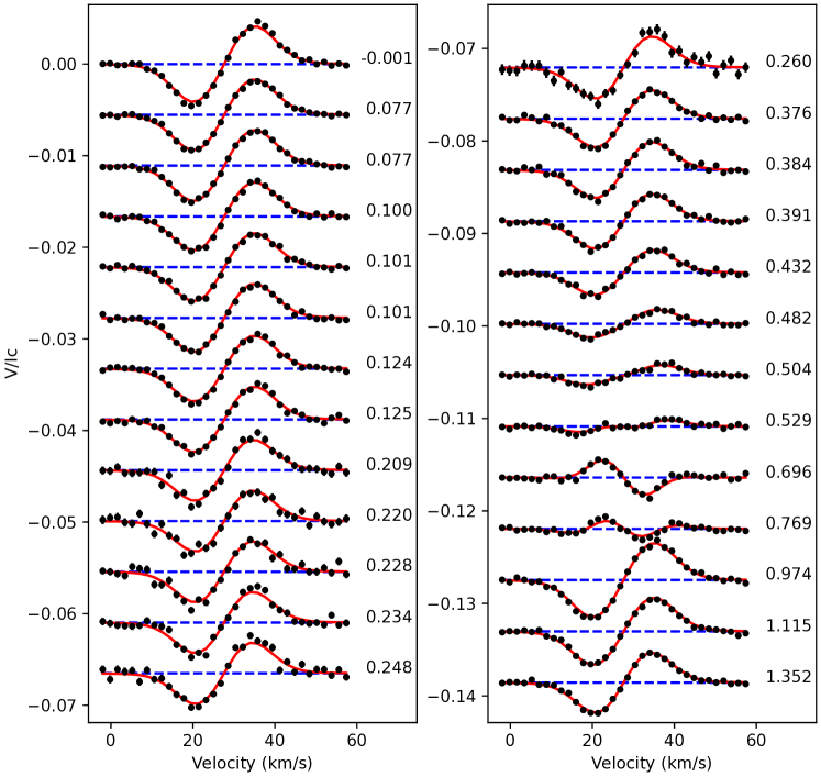
Figure 8: ZDI model fits (red) to the observed Stokes $V$ LSD profiles (black). Rotation cycles are labeled on the right. Profiles are shifted vertically for clarity. Error bars are plotted but are often smaller than the points.

The ZDI model line requires a wavelength and effective Landé factor, which were set to the normalizing values for the LSD profile (500 nm and 1.2). A limb darkening coefficient of 0.33 was used (Claret & Bloemen, 2011), which implies a slope for the source function in the Unno-Rachkovsky model of 0.4925. The local line opacity profile Gaussian width (combination of thermal and turbulent broadening), Lorentzian width (pressure broadening), and strength were fit using the Stokes $I$ and $V$ profiles. Additional broadening by a Gaussian instrumental profile of $R=65000$ was assumed. The strong magnetic field produces a non-negligible amount of broadening in Stokes $I$, thus this fitting process was done iteratively with the magnetic mapping process described below. The Gaussian (thermal + turbulent) broadening dominates the total line broadening, but is $\sim$1 km s^-1 smaller in our final model than suggested by a non-magnetic model. The final Gaussian width was 7.2 km s^-1 ($\sqrt{2}\sigma$ of the Gaussian), as the midpoint between optimal values for Stokes $I$ and Stokes $V$. This range leads to a potential systematic uncertainty of $\pm 0.5$ km s^-1, which spans the optimal values for Stokes $I$ and $V$. The Lorentzian width was 1.1 km s^-1 ($\gamma$, half-width at half-maximum).

The very low $v\sin i$ of HD 54879 limits the information that can be reconstructed with ZDI. Smaller surface features, corresponding to higher degree spherical harmonics, are not resolved in the Stokes $V$ observations. However, even lacking Doppler resolution, the few lowest degree spherical harmonics can be resolved by rotational modulation with dense phase coverage. We restricted the maximum degree $l$ of the reconstructed spherical harmonics to $l_{\rm max}=5$. In testing a larger $l_{\rm max}$, the higher degree spherical harmonic coefficients tended to 0 due to the regularization. Even modes with $l>3$ had relatively small coefficients, suggesting we have little sensitivity to these modes. The toroidal components of the magnetic field are also virtually undetectable in Stokes $V$ at this $v\sin i$. At higher $v\sin i$ the toroidal components are mostly detectable in $V$ towards the limb of the star as regions of field with opposite orientation, but when $v\sin i$ $=0$ these regions cancel out. Consequently we restricted the magnetic geometry to a potential poloidal field. In terms of the vector spherical harmonic coefficients defined by Donati et al. (2006) (equations [2-4]), this restriction is equivalent to setting $\alpha_{l,m}=\beta_{l,m}$ and $\gamma_{l,m}=0$. If we allow the toroidal field to be free, it tends towards 0 due to the regularization; but this does not represent an absence of toroidal field, only our lack of sensitivity to this field component.

The inclination of the rotation axis ($i$) is a significant uncertainty for this magnetic mapping. We fixed $i$ by searching for the value that optimizes the ZDI result. We ran a grid of ZDI models varying $i$ from $1^{\circ}$ to $90^{\circ}$ (in steps of $1^{\circ}$), with $v_{\rm eq}=0.12$ km s^-1, and chose the model with the highest entropy that converged the target $\chi_{\nu}^{2}$ (set to 1.5). To find a formal uncertainty on this inclination we repeated the grid search, but instead ran the code fitting to a target entropy rather than target $\chi_{\nu}^{2}$, with the target entropy set to the previous best value. This produced a curve of $\chi_{\nu}^{2}$ as a function of $i$, for models with the same entropy, and the variation in $\chi_{\nu}^{2}$ about the minimum can be used to estimate an uncertainty. This follows the procedure of Petit et al. (2002), discussed more by Folsom et al. (2018a) for $i$, and the approach was found to work well for cool stars with very low $v\sin i$ by Folsom et al. (2018b) and Folsom et al. (2020). This produced a best inclination of $i=74\pm 3^{\circ}$, although this may underestimate the real uncertainty due to the very high S/N of the LSD profiles. Varying the Gaussian line width by $\pm 0.5$ km s^-1 varies $i$ by at most $1^{\circ}$, so this is a small contribution to the $i$ uncertainty. Varying $v_{\rm eq}$ by its $\pm 0.03$ km s^-1 uncertainty, varying the rotation period by its uncertainty, or changing the limb darkening coefficient by $\pm 0.1$, all change $i$ by less than $1^{\circ}$.

We used a similar grid search approach to verify the rotation period, following Petit et al. (2002). Running a grid of ZDI models for a range of periods, we find $P=2580\pm 30$ d, which is in good agreement with the value from $\langle B_{z}\rangle$ of $2562^{+63}_{-58}$ d. Since the period from the ZDI search is more model dependent, and subject to more systematic uncertainties that are harder to quantify, we adopt the period from $\langle B_{z}\rangle$ in the ZDI analysis and the rest of this study.

3.5.3 The magnetic map

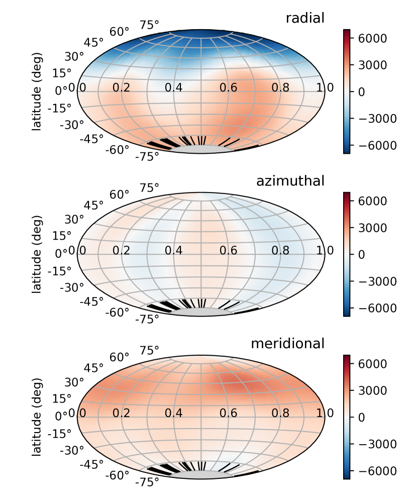
Figure 9: Magnetic map from ZDI for the radial, azimuthal, and meridional components of the magnetic field. Presented in a Hammer projection with coordinates of latitude and rotation phase. The color scale gives magnetic field in G. Ticks at the bottom indicate phases of observations. The grey area is the unobservable portion of the star.

Table 2: Parameters describing the magnetic map.

stellar parameter	value
P	$2562^{+63}_{-58}$ d
$v\sin i$	$0.116\pm 0.029$ km s-1
$i$	$74\pm 3$°
magnetic parameter	value
mean $|B|$	2954 G
maximum $|B|$	6961 G
dipole $B_{p}$	3939 G
dipole obliquity	168°
quadrupole $B_{\rm max}$	2299 G
quadrupole $B_{\rm min}$	-2331 G
quadrupole max. locations	87°, 114°
(colatitude, longitude)	93°, 294°
quadrupole min. locations	9°, 7°
(colatitude, longitude)	171°, 187°
dipolar energy	74%
quadrupolar energy	23%
octupolar energy	2%
total axisymmetry	89%
dipolar axisymmetry	96%
quadrupolar axisymmetry	72%

The final best fit to the Stokes $V$ LSD profiles is shown in Figure 8, and the corresponding magnetic map is shown in Figure 9. This result fits the data to $\chi_{\nu}^{2}=1.5$, which we consider acceptable given the small error bars in the LSD profiles. The surface average magnetic field strength is 2954 G, reaching a maximum of 6961 G at a point 20^∘ from the rotation axis near phase 0. The dipole component has a polar strength of 3939 G and obliquity of the positive pole relative to the rotation axis of 168^∘ at a longitude of 128° (phase 0.64; rotation phase runs in the opposite direction to longitude in this model). The magnetic geometry can be described in terms of the fraction of magnetic energy (proportional to $\oint B^{2}\,d\Omega$) in different spherical harmonic components. We find 74% of the magnetic energy in the dipole ($l=1$) components, 23% in the quadrupole (l=2) components and 2% in the octupole (l=3) components. The field is largely axisymmetric (about the rotation axis) with 89% of the energy in axisymmetric ($m=0$) components. Parameters describing the magnetic field are presented in Table 2.

The very low $v\sin i$ of HD 54879 leads to some large uncertainties in the magnetic map. Most obviously, only the largest scale components of the magnetic field are reconstructed. Components up to the octupole are resolved through the good rotation phase coverage, but beyond that (for $l>3$) the geometry is largely unresolved. The toroidal components of the magnetic field are similarly unresolved, due to the lack of Doppler resolution. The toroidal field is typically weak in O and B stars (e.g. Grunhut et al., 2022), but in a few cases it is important (Donati et al., 2006).

The uncertainty on $v\sin i$ has a negligible impact on the magnetic field model, as do likely variations in the limb darkening coefficient. Varying the rotation period by $\pm 1\sigma$ changes the magnetic field strength and geometry (energy fractions) by less than 1%. Increasing the inclination by $1\sigma$ increases the magnetic field strength by $\sim$500 G and shifts 10% of the energy into the dipole component. Decreasing the inclination by the same amount decreases the magnetic field strength by $\sim$500 G but shifts 20% of the dipolar energy to higher multipoles. Increasing the Gaussian width by $0.5$ km s^-1 increases the magnetic field strength by $\sim$100 G and shifts $\sim$3% of the magnetic energy away from the dipole, and also causes the ZDI code to converge very slowly to the target $\chi_{\nu}^{2}$ of 1.5 (implying possible over-fitting, and that for this parameter combination a larger target $\chi_{\nu}^{2}$ likely should be chosen). Decreasing the Gaussian width by $0.5$ km s^-1 decreases the magnetic field strength by $\sim$30 G, and shifts the magnetic energy towards the dipole by $\sim$1%.

The variation in H$\alpha$ equivalent width correlates with the magnetic field map. The maxima in H$\alpha$ emission occur near phases 0.1 and 0.6, which correspond to places where the positive radial field crosses above the equator, and maxima in the meridional field occur. Minima in H$\alpha$ emission occur near phases 0.4 and 0.9, where the negative radial field spans the largest latitude range. This correlation between surface magnetic field structure and H$\alpha$ emission strongly suggests that the stellar wind is being influenced by the magnetic field. Material from the wind can become trapped in closed magnetic field loops above the surface of the star, leading to enhanced H$\alpha$ emission. HD 54879 has been noted to have an unusually strong H$\alpha$ emission for its spectral type (Boyajian et al., 2007; Castro et al., 2015). This could be explained by the very strong axisymmetric dipolar component of the magnetic field, which should lead to large closed field loops being observable at all rotation phases. Modeling of the magnetosphere around the star is needed to fully explore this hypothesis, such as the Analytic Dynamical Magnetosphere approach (Owocki et al., 2016; Munoz et al., 2020) or MHD simulations.

4 Discussion and Conclusions

The most recent spectropolarimetric data of HD 54879 indicate that the longitudinal magnetic field has once again reached the negative magnetic extremum and begun increasing, implying the full stellar rotation period has now been observed. Our best empirical fit to the longitudinal field data yields a stellar rotation period of $\mathrm{P}=2562^{+63}_{-58}$ d, which is about 7.02 yr.

We revisited the longitudinal magnetic field variation measured from LSD profiles constructed from lines of individual elements, specifically He, O and Si. While those longitudinal field curves show some small differences in amplitude, their similar shapes, compounded by the lack of any significant line profile or EW variability of these elements, leads us to attribute these discrepancies to small differences in the measurement systems associated with the different line masks. In contrast to Järvinen et al. (2022), we see no evidence for chemical stratification or lateral abundance nonuniformities.

Unlike the majority of other known magnetic O stars, HD 54879’s longitudinal field curve shows significant evidence for a complex magnetic topology with a strong quadrupolar component. This is supported by the magnetic map for HD 54879 that we present – the first magnetic map of this star – which suggests a surface-averaged magnetic field strength of 2954 G. The dipole component has a polar strength of 3939 G and is nearly aligned with the rotation axis ($\beta=168$°). There is a relatively large quadrupolar component to the magnetic field, with 74% of the magnetic energy in the dipole, and 23% in quadrupolar components. HD 54879 is indeed one of the most strongly magnetic O-type stars identified to date.

In parallel, we also investigated how H$\alpha$ emission varies with rotation, finding that the equivalent width of the line varies fairly coherently with $\langle B_{z}\rangle$. The correlation between the magnetic results and the equivalent widths overall supports the interpretation that the variability in H$\alpha\;$is largely driven by a magnetically confined wind. We present a fit to the H$\alpha\;$equivalent widths using the rotation period derived from $\langle B_{z}\rangle$. However, assuming that these variations are rotationally modulated, an independent fit using a 2-component harmonic function yields a different (longer) period, albeit within the same order of magnitude. While additional stellar monitoring will be needed to resolve this discrepancy, we conclude that the H$\alpha$ equivalent width variation supports the notion that HD 54879 is an extreme slow rotator: the magnetic O-type star with the second longest rotational period known to this day.

Some properties of the magnetosphere can be estimated without detailed modeling. ud-Doula et al. (2008) provide a method for calculating an approximate Alfvén radius ($R_{A}$) using their wind confinement parameter ($\eta_{*}$). For this we used the prescription of Vink et al. (2001) to estimate a theoretical mass-loss rate in the absence of a magnetic field ($\dot{M}_{B=0}$), and followed their recommendation for the terminal wind speed ($v_{\infty}$) as 2.6 of the escape velocity (Lamers et al., 1995). We used $T_{\rm eff}=30500$ K, $\log L/L_{\odot}=4.45$, $R_{*}=6.1~{}R_{\odot}$, and $M_{*}=14~{}M_{\odot}$ from Shenar et al. (2017), to estimate $\log\dot{M}_{B=0}=-7.9$ $[M_{\odot}~{}\textrm{yr}^{-1}]$ and $v_{\infty}=2400$ km s^-1. We used the dipole approximation of ud-Doula et al. (2008) with our dipolar component field strength (3939 G at the pole, 1970 G at the equator), although this neglects some magnetic field strength and complexity, which leads to $\eta_{*}=3500$ and $R_{A}/R_{*}=8.0$. In contrast, the Kepler radius (ud-Doula et al., 2008), calculated with our period, is $R_{K}/R_{*}=310$. The places HD 54879 in an unusual position in the classification scheme of Petit et al. (2013), where $R_{A}$ is large (larger than all other O stars from Petit et al. 2013), but still much smaller than $R_{K}$. This implies that there is a large volume of trapped magnetosphere material, which is not supported against gravity by rotation, and indeed rotation is nearly negligible.

The large Alfvén radius will substantially reduce the real mass-loss rate. Using the dipole approximation from ud-Doula et al. (2008) we calculated the reduction in mass-loss rate due to the magnetic field $\dot{M}/\dot{M}_{B=0}=0.09$ ($\log\dot{M}=-8.9~{}[M_{\odot}\textrm{yr}^{-1}]$), although this may be sensitive to the magnetic geometry. The large $R_{A}$ also implies significant angular momentum loss and relatively short spindown timescale (ud-Doula et al., 2009; Petit et al., 2013) of $\tau_{J}=\sim 2.6$ Myr. However, accounting for the current very slow rotation of the star, the spindown age (the age the star would have if it began its life at critical rotation and braked steadily to the current value; Petit et al. 2013) is $t_{J}\sim 22$ Myr. This is discrepant with the ages of 4 or 5 Myr (Castro et al., 2015; Shenar et al., 2017) from comparisons with non-magnetic evolutionary tracks. While the star may have reached the main sequence as a very slow rotator, this may indicate a need for a more careful assessment of the stellar age and spindown timescale.

There is a large uncertainty in the wind parameters. Shenar et al. (2017) attempted to derive $\dot{M}_{B=0}$ from observations, using spherically symmetric models but including an approximate treatment of the effects of the magnetic field. They found $\log\dot{M}_{B=0}=9.0~{}[M_{\odot}\textrm{yr}^{-1}]$ and $v_{\infty}=1700$ km s^-1, which are both much smaller than the theoretical values of Vink et al. (2001). If we adopt these values from Shenar et al. (2017) that leads to $\eta_{*}=65000$, $R_{A}/R_{*}=16.0$, $\dot{M}/\dot{M}_{B=0}=0.04$, $\log\dot{M}=-10.4~{}[M_{\odot}\textrm{yr}^{-1}]$, $\tau_{J}=\sim 8.3$ Myr, and $t_{J}\sim 71$ Myr. Thus the weaker wind would lead to an Alfvén radius twice as large, but a spindown timescale and age that are $\sim 3\times$ longer, and in stronger conflict with the age from evolutionary tracks.

The evolutionary history of HD 54879 has yet to be fully explored. Previous work by Castro et al. (2015) and Shenar et al. (2017) used the Bayesian statistical tool and method BONNSAI (Schneider et al., 2014) to infer the age of HD 54879. This method infers the probability distribution of stellar parameters such as age via the comparison of observables to any set of stellar evolution models. Both studies used a set of main-sequence, single, non-magnetic massive star evolution models with Milky Way compositions that were produced by Brott et al. (2011). There was statistical agreement between the inferred ages of $5\pm 1$ Myr (Shenar et al., 2017) and $4.0^{+0.8}_{-1.2}$ (Castro et al., 2015). Additionally, Shenar et al. (2017) inferred an initial mass of $16\pm 1M_{\odot}$. However, these models do not account for the effects of magnetic fields such as the reduction of mass loss with respect to evolutionary time scales, so there are added uncertainties that have not been evaluated. Acknowledging the results of this work, which reveal the complex magnetic topology of the star, suggests that these previous estimates will need to be revised.

Data Availability Statement

The data used in this work can be accessed via the public archives maintained by the Canadian Astronomy Data Centre (ESPaDOnS; https://www.cadc-ccda.hia-iha.nrc-cnrc.gc.ca/en/), by Polarbase (ESPaDOnS and Narval; http://polarbase.irap.omp.eu/), or by request of the authors.

References

- Aurière (2003) Aurière, M. 2003, in EAS Publications Series, Vol. 9, EAS Publications Series, ed. J. Arnaud & N. Meunier, 105
- Bellotti et al. (2023) Bellotti, S., Morin, J., Lehmann, L. T., et al. 2023, A&A, 676, A56, doi: 10.1051/0004-6361/202346845
- Boyajian et al. (2007) Boyajian, T. S., Gies, D. R., Baines, E. K., et al. 2007, PASP, 119, 742, doi: 10.1086/520707
- Brott et al. (2011) Brott, I., de Mink, S. E., Cantiello, M., et al. 2011, A&A, 530, A115, doi: 10.1051/0004-6361/201016113
- Castro et al. (2015) Castro, N., Fossati, L., Hubrig, S., et al. 2015, A&A, 581, A81, doi: 10.1051/0004-6361/201425354
- Charbonneau (2013) Charbonneau, P. 2013, Solar and Stellar Dynamos, Saas-Fee Advanced Course, doi: 10.1007/978-3-642-32093-4
- Claret & Bloemen (2011) Claret, A., & Bloemen, S. 2011, A&A, 529, A75, doi: 10.1051/0004-6361/201116451
- David-Uraz et al. (2021) David-Uraz, A., Petit, V., Shultz, M. E., et al. 2021, MNRAS, 501, 2677, doi: 10.1093/mnras/staa3768
- Donati & Brown (1997) Donati, J. F., & Brown, S. F. 1997, A&A, 326, 1135
- Donati et al. (1997) Donati, J. F., Semel, M., Carter, B. D., Rees, D. E., & Collier Cameron, A. 1997, MNRAS, 291, 658, doi: 10.1093/mnras/291.4.658
- Donati et al. (2006) Donati, J. F., Howarth, I. D., Jardine, M. M., et al. 2006, MNRAS, 370, 629, doi: 10.1111/j.1365-2966.2006.10558.x
- Donati et al. (2008) Donati, J. F., Jardine, M. M., Gregory, S. G., et al. 2008, MNRAS, 386, 1234, doi: 10.1111/j.1365-2966.2008.13111.x
- Erba et al. (2021) Erba, C., David-Uraz, A., Petit, V., et al. 2021, Monthly Notices of the Royal Astronomical Society, 506, 5373, doi: 10.1093/mnras/stab1853
- Folsom et al. (2020) Folsom, C. P., Ó Fionnagáin, D., Fossati, L., et al. 2020, A&A, 633, A48, doi: 10.1051/0004-6361/201937186
- Folsom et al. (2018a) Folsom, C. P., Bouvier, J., Petit, P., et al. 2018a, MNRAS, 474, 4956, doi: 10.1093/mnras/stx3021
- Folsom et al. (2018b) Folsom, C. P., Fossati, L., Wood, B. E., et al. 2018b, MNRAS, 481, 5286, doi: 10.1093/mnras/sty2494
- Fossati et al. (2015) Fossati, L., Castro, N., Schöller, M., et al. 2015, A&A, 582, A45, doi: 10.1051/0004-6361/201526725
- Georgy et al. (2017) Georgy, C., Meynet, G., Ekström, S., et al. 2017, A&A, 599, L5, doi: 10.1051/0004-6361/201730401
- Gray (2005) Gray, D. F. 2005, The Observation and Analysis of Stellar Photospheres, 3rd edn. (Cambridge, UK: Cambridge University Press)
- Grunhut et al. (2017) Grunhut, J. H., Wade, G. A., Neiner, C., et al. 2017, MNRAS, 465, 2432, doi: 10.1093/mnras/stw2743
- Grunhut et al. (2022) Grunhut, J. H., Wade, G. A., Folsom, C. P., et al. 2022, MNRAS, 512, 1944, doi: 10.1093/mnras/stab3320
- Hobson & Lasenby (1998) Hobson, M. P., & Lasenby, A. N. 1998, MNRAS, 298, 905, doi: 10.1046/j.1365-8711.1998.01707.x
- Holgado et al. (2022) Holgado, G., Simón-Díaz, S., Herrero, A., & Barbá, R. H. 2022, A&A, 665, A150, doi: 10.1051/0004-6361/202243851
- Hubrig et al. (2020) Hubrig, S., Järvinen, S. P., Schöller, M., & Hummel, C. A. 2020, MNRAS, 491, 281, doi: 10.1093/mnras/stz3046
- Hubrig et al. (2019) Hubrig, S., Küker, M., Järvinen, S. P., et al. 2019, MNRAS, 484, 4495, doi: 10.1093/mnras/stz198
- Järvinen et al. (2022) Järvinen, S. P., Hubrig, S., Schöller, M., et al. 2022, MNRAS, 510, 4405, doi: 10.1093/mnras/stab3720
- Järvinen et al. (2021) —. 2021, MNRAS, 501, 4534, doi: 10.1093/mnras/staa3919
- Keszthelyi (2023) Keszthelyi, Z. 2023, Galaxies, 11, 40, doi: 10.3390/galaxies11020040
- Keszthelyi et al. (2019) Keszthelyi, Z., Meynet, G., Georgy, C., et al. 2019, MNRAS, 485, 5843, doi: 10.1093/mnras/stz772
- Keszthelyi et al. (2021) Keszthelyi, Z., Meynet, G., Martins, F., de Koter, A., & David-Uraz, A. 2021, MNRAS, 504, 2474, doi: 10.1093/mnras/stab893
- Keszthelyi et al. (2020) Keszthelyi, Z., Meynet, G., Shultz, M. E., et al. 2020, MNRAS, 493, 518, doi: 10.1093/mnras/staa237
- Keszthelyi et al. (2022) Keszthelyi, Z., de Koter, A., Götberg, Y., et al. 2022, MNRAS, 517, 2028, doi: 10.1093/mnras/stac2598
- Kochukhov et al. (2011) Kochukhov, O., Lundin, A., Romanyuk, I., & Kudryavtsev, D. 2011, ApJ, 726, 24, doi: 10.1088/0004-637X/726/1/24
- Kochukhov et al. (2010) Kochukhov, O., Makaganiuk, V., & Piskunov, N. 2010, A&A, 524, A5, doi: 10.1051/0004-6361/201015429
- Kupka et al. (1999) Kupka, F., Piskunov, N., Ryabchikova, T. A., Stempels, H. C., & Weiss, W. W. 1999, A&AS, 138, 119, doi: 10.1051/aas:1999267
- Kupka et al. (2000) Kupka, F. G., Ryabchikova, T. A., Piskunov, N. E., Stempels, H. C., & Weiss, W. W. 2000, Baltic Astronomy, 9, 590, doi: 10.1515/astro-2000-0420
- Lamers et al. (1995) Lamers, H. J. G. L. M., Snow, T. P., & Lindholm, D. M. 1995, ApJ, 455, 269, doi: 10.1086/176575
- Landi Degl’Innocenti & Landolfi (2004) Landi Degl’Innocenti, E., & Landolfi, M. 2004, Astrophysics and Space Science Library, Vol. 307, Polarization in Spectral Lines (Dordrecht: Kluwer Academic Publishers), doi: 10.1007/978-1-4020-2415-3
- Marcolino et al. (2013) Marcolino, W. L. F., Bouret, J. C., Sundqvist, J. O., et al. 2013, MNRAS, 431, 2253, doi: 10.1093/mnras/stt323
- Meynet et al. (2011) Meynet, G., Eggenberger, P., & Maeder, A. 2011, A&A, 525, L11, doi: 10.1051/0004-6361/201016017
- Morel et al. (2015) Morel, T., Castro, N., Fossati, L., et al. 2015, in IAU Symposium, Vol. 307, New Windows on Massive Stars, ed. G. Meynet, C. Georgy, J. Groh, & P. Stee, 342–347, doi: 10.1017/S1743921314007054
- Morin et al. (2008) Morin, J., Donati, J. F., Petit, P., et al. 2008, MNRAS, 390, 567, doi: 10.1111/j.1365-2966.2008.13809.x
- Munoz et al. (2020) Munoz, M. S., Wade, G. A., Nazé, Y., et al. 2020, MNRAS, 492, 1199, doi: 10.1093/mnras/stz2904
- Nazé et al. (2001) Nazé, Y., Vreux, J.-M., & Rauw, G. 2001, A&A, 372, 195, doi: 10.1051/0004-6361:20010473
- Owocki et al. (2016) Owocki, S. P., ud-Doula, A., Sundqvist, J. O., et al. 2016, MNRAS, 462, 3830, doi: 10.1093/mnras/stw1894
- Petit et al. (2002) Petit, P., Donati, J. F., & Collier Cameron, A. 2002, MNRAS, 334, 374, doi: 10.1046/j.1365-8711.2002.05529.x
- Petit et al. (2013) Petit, V., Owocki, S. P., Wade, G. A., et al. 2013, MNRAS, 429, 398, doi: 10.1093/mnras/sts344
- Petit et al. (2017) Petit, V., Keszthelyi, Z., MacInnis, R., et al. 2017, MNRAS, 466, 1052, doi: 10.1093/mnras/stw3126
- Piskunov & Kochukhov (2002) Piskunov, N., & Kochukhov, O. 2002, A&A, 381, 736, doi: 10.1051/0004-6361:20011517
- Piskunov et al. (2011) Piskunov, N., Snik, F., Dolgopolov, A., et al. 2011, The Messenger, 143, 7
- Piskunov et al. (1995) Piskunov, N. E., Kupka, F., Ryabchikova, T. A., Weiss, W. W., & Jeffery, C. S. 1995, A&AS, 112, 525
- Rauw et al. (2023) Rauw, G., Nazé, Y., ud-Doula, A., & Neiner, C. 2023, MNRAS, 521, 2874, doi: 10.1093/mnras/stad693
- Ryabchikova et al. (2015) Ryabchikova, T., Piskunov, N., Kurucz, R. L., et al. 2015, Phys. Scr, 90, 054005, doi: 10.1088/0031-8949/90/5/054005
- Ryabchikova et al. (1997) Ryabchikova, T. A., Piskunov, N. E., Kupka, F., & Weiss, W. W. 1997, Baltic Astronomy, 6, 244, doi: 10.1515/astro-1997-0216
- Schneider et al. (2014) Schneider, F. R. N., Langer, N., de Koter, A., et al. 2014, A&A, 570, A66, doi: 10.1051/0004-6361/201424286
- Schneider et al. (2020) Schneider, F. R. N., Ohlmann, S. T., Podsiadlowski, P., et al. 2020, MNRAS, 495, 2796, doi: 10.1093/mnras/staa1326
- Schneider et al. (2019) Schneider, F. R. N., Ohlmann, S. T., Podsiadlowski, P., et al. 2019, Nature, 574, 211, doi: 10.1038/s41586-019-1621-5
- Shenar et al. (2017) Shenar, T., Oskinova, L. M., Järvinen, S. P., et al. 2017, A&A, 606, A91, doi: 10.1051/0004-6361/201731291
- Shultz & Wade (2017) Shultz, M., & Wade, G. A. 2017, MNRAS, 468, 3985, doi: 10.1093/mnras/stx759
- Shultz et al. (2018) Shultz, M. E., Wade, G. A., Rivinius, T., et al. 2018, MNRAS, 475, 5144, doi: 10.1093/mnras/sty103
- Shultz et al. (2019) —. 2019, MNRAS, 490, 274, doi: 10.1093/mnras/stz2551
- Silvester et al. (2014) Silvester, J., Kochukhov, O., & Wade, G. A. 2014, MNRAS, 440, 182, doi: 10.1093/mnras/stu306
- Skilling & Bryan (1984) Skilling, J., & Bryan, R. K. 1984, MNRAS, 211, 111, doi: 10.1093/mnras/211.1.111
- Sota et al. (2011) Sota, A., Maíz Apellániz, J., Walborn, N. R., et al. 2011, ApJS, 193, 24, doi: 10.1088/0067-0049/193/2/24
- Sundqvist et al. (2012) Sundqvist, J. O., ud-Doula, A., Owocki, S. P., et al. 2012, MNRAS, 423, L21, doi: 10.1111/j.1745-3933.2012.01248.x
- ud-Doula & Owocki (2002) ud-Doula, A., & Owocki, S. P. 2002, ApJ, 576, 413, doi: 10.1086/341543
- ud-Doula et al. (2008) ud-Doula, A., Owocki, S. P., & Townsend, R. H. D. 2008, MNRAS, 385, 97, doi: 10.1111/j.1365-2966.2008.12840.x
- ud-Doula et al. (2009) —. 2009, MNRAS, 392, 1022, doi: 10.1111/j.1365-2966.2008.14134.x
- ud-Doula et al. (2013) ud-Doula, A., Sundqvist, J. O., Owocki, S. P., Petit, V., & Townsend, R. H. D. 2013, MNRAS, 428, 2723, doi: 10.1093/mnras/sts246
- Vink et al. (2001) Vink, J. S., de Koter, A., & Lamers, H. J. G. L. M. 2001, A&A, 369, 574, doi: 10.1051/0004-6361:20010127
- Wade et al. (2000) Wade, G. A., Donati, J. F., Landstreet, J. D., & Shorlin, S. L. S. 2000, MNRAS, 313, 851, doi: 10.1046/j.1365-8711.2000.03271.x
- Wade et al. (2011) Wade, G. A., Howarth, I. D., Townsend, R. H. D., et al. 2011, MNRAS, 416, 3160, doi: 10.1111/j.1365-2966.2011.19265.x
- Wade et al. (2016) Wade, G. A., Neiner, C., Alecian, E., et al. 2016, MNRAS, 456, 2, doi: 10.1093/mnras/stv2568
- Wade et al. (2020) Wade, G. A., Bagnulo, S., Keszthelyi, Z., et al. 2020, MNRAS, 492, L1, doi: 10.1093/mnrasl/slz174
- Walborn et al. (2010) Walborn, N. R., Sota, A., Maíz Apellániz, J., et al. 2010, ApJ, 711, L143, doi: 10.1088/2041-8205/711/2/L143
- Yakunin et al. (2015) Yakunin, I., Wade, G., Bohlender, D., et al. 2015, MNRAS, 447, 1418, doi: 10.1093/mnras/stu2401