X-ray Iron absorption line in Swift J1858.6–0814

Abstract

We present the spectral analysis of bright steady states in an outburst of the transient neutron star low-mass X-ray binary (NS-LMXB) Swift J1858.6$-$0814 observed with NICER. We detected an ionized iron K absorption line (H-like Fe) at 6.97 keV in the spectrum. We estimated the photoionization parameter using the ratio of the equivalent widths (EWs) of the Fe XXVI (H-like) ($17\pm 5$ eV) and Fe XXV (He-like) ($<3$ eV) and discuss the origin of the iron absorption line. The irradiated gas producing the absorption line would locate within (3–6)$\times 10^{9}{\rm cm}$ from the X-ray source. We suggest that the observed H-like Fe absorption line originates from the highly-ionized gas in the inner accretion disk in Swift J1858.6$-$0814.

1 Introduction

The transient neutron star low mass X-ray binary (NS-LMXB) Swift J1858.6$-$0814 was discovered with Swift/BAT on 2018 October 25 (Krimm et al., 2018). In the X-ray spectrum with XMM-Newton Reflection Grating Spectrometer (RGS), Buisson et al. (2020a) found emission lines from Ne IX, O VII, O VIII, and N VII, which indicate the existence of the photoionized gas around Swift J1858.6$-$0814. They reported that these could be associated either with the disk atmosphere as in accretion disk corona (ADC) source, or with the wind, because of the red-shifted N VII emission line, which is consistent with an emission line of P-Cygni profile. The emitting plasma had an ionization parameter $\log_{10}(\xi)=1.35\pm 0.2$ and a number density $n>1.5\times 10^{11}$cm^-3. Here, the ionization parameter $\xi$ is

$$\xi=\frac{L}{nR^{2}}$$ (1)

where $L$ is the ionizing X-ray luminosity, $n$ is the number density of the irradiated gas, and $R$ is the distance from the X-ray source. From these parameters, they inferred that the emitting plasma must be within $10^{13}$ cm from the ionizing X-ray source, and also that it is at least $>2\times 10^{9}$  cm from the line width. Buisson et al. (2020b) detected five thermonuclear (Type I) X-ray bursts from Swift J1858.6$-$0814, implying that the compact object in the system is a NS. Some of the bursts showed photospheric radius expansion, and their results give several system parameters; a high inclination and a helium atmosphere for the most likely values, although systematic effect allows a conservative range of 9–18 kpc in the distance. They also detected mHz QPOs (quasi-periodic oscillations) before one burst. The mHz QPO has an average frequency of $9.6\pm 0.5$ mHz and a fractional rms amplitude of $2.2\pm 0.2$ per cent (0.5–10 keV).

Buisson et al. (2021) discovered the eclipses and several absorption dips during the pre-eclipse phase in NICER data. From these, an orbital period $P=76841.3^{+1.3}_{-1.4}$ s ($\sim 21.3$ h), an eclipse duration of $t_{\rm ec}=4098^{+17}_{-18}$ s ($\sim 1.14$ h) were derived. The inclination of the binary orbit was constrained to $i>$70D. Knight et al. (2022) analyzed X-ray eclipses in NICER data and constrained the binary inclination and mass ratio. An ablation layer on the companion-star surface was introduced to explain the energy-dependent and asymmetric ingress and egress. The obtained inclination and mass ratio were $i\sim 81^{\circ}$ and $q\sim 0.14$, respectively. The companion mass and radius were determined in the range of 0.183 – 0.372   and 1.02 – 1.29 $R_{\odot}$, respectively. The average spectrum shows an ionized iron K absorption line at 6.97 keV in figure 3 and table 1 in Knight et al. (2022).

Recently X-ray binaries have often been observed to have several absorption lines from highly ionized iron, such as Fe XXVI (H-like), Fe XXV (He-like) (table 5 in Boirin et al. (2004), Ueda et al. (2004)). These results indicate that highly ionized plasma is often present in the binary system. The existence of highly ionized plasma also suggests that LMXB has accretion disk atmosphere and/or disk wind. Clear observational evidence for strong disk wind has so far been seen in several LMXBs (e.g., a summary by Díaz Trigo and Boirin (2016)).

In this paper, using the absorption line we estimated the location and the size of the irradiated gas producing the absorption line. First, we reanalyze the NICER data of Swift J1858.6–0814 in section 2 and show the results in section 3. We confirm the iron absorption line in section 4. Then we discuss the column densities and the location of the absorbing ionized plasma using the ratio of the equivalent widths (EWs) of the Fe XXVI (H-like) and Fe XXV (He-like) in section 5 and summarize in section 6.

2 Observations and data analysis

We obtained long-term light curves of MAXI/GSC (MAXI: Matsuoka et al. (2009), Gas Slit Camera: Mihara et al. (2011); Sugizaki et al. (2011)) including the period of an outburst of Swift J1858.6$-$0814 (MJD = 58800–59000) from the MAXI mission website. Next, we inspected the NICER (Gendreau et al., 2016) light curves, and selected the period of bright steady states in an outburst for the spectral analysis. The data are reduced using the NICER data reduction software (HEASOFT V6.30.1, CALDB 20210707). We used the NICER data of 35 OBSIDs, which covers observations from 2020 March 3 (MJD = 58911) to 29 (MJD = 58938). A light curve and an average spectrum were created from the merged 35 cleaned event files provided by the NICER team. The light curves of Swift J1858.6$-$0814 are shown in figure 1. In the top panel (MAXI/GSC light curve), the dotted lines indicate the span of the NICER data (MJD = 58911–58922), when the source was bright enough for the spectrum analysis. In the bottom panel (NICER light curve), the inset square indicates the data region that we used for the spectrum analysis, where the count rate is 140–300 counts s^-1.

We make a time-average spectrum from the data of the square region. Here, the background modeling was done using ”nibackgen3C50” task provided by the NICER team. Respons files were created by ”nicerarf” and ”nicerrmf” task provided by the NICER team.

Figure 1: The top panel is a MAXI/GSC light curve of 4–10 keV including the outburst in 1 day bin. The dotted lines indicate the span of the NICER data that we used. The bottom panel is a NICER light curve of 0.7–10 keV in 16 s bin. The inset square is the data region that we used.

In the spectral analysis of the time-averaged spectrum, we used models in XSPEC V12.12.1 (Arnaud, 1996). First, we use the typical two-component spectral model of NS-LMXB for the continuum component.

One component (bbodyrad) accounts for a blackbody spectrum from the central source (NS), and the other (diskbb)(Mitsuda et al., 1984) is the multi-temperature blackbody spectrum originating from the inner accretion disk. Here, we assume that the Compton cloud completely covers the emission region for the hard component (bbodyrad), and use Thcomp * bbodyrad model. It describes Comptonized spectrum by thermal electrons (Zdziarski et al., 2020) of blackbody emission from the central source. We also introduce the gaussian model for the emission line between 6–7 keV, which is often observed in binary systems. For absorption by the intervening medium, we used TBabs model described a neutral absorber with the abundance by Wilms et al. (2000). For iron absorption line detected by Knight et al. (2022), the gabs model is used. Here, We fix the line width of the gabs at 0.05 keV, which is narrow enough for the detector energy resolution, but still broad enough for the response channel resolution. We fit the time-averaged spectrum with the model, TBabs*gabs*(Thcomp*bbodyrad+diskbb+gaussian) .

Figure 2: NICER spectrum fitted with the multi-component model. The top and middle panels are for the best fit. The bottom panel is that spectrum without the three low-energy emission lines and the ionized absorber. The dotted lines show the individual spectral components. The hard broad component shows bbodyrad and the soft one show diskbb. Four narrow gaussian components show four emission lines. See the text in detail.

The fitting yields significant residuals in 1–2keV (bottom panel in fig 2). The reduced $\chi^{2}$ is $\chi^{2}/\nu=2.41$ with d.o.f of 292, which is not acceptable. Hence, we tried to the partial covering absorption model because the time-average spectrum may contain absorption components with different column densities. However, for the partial covering model by neutral absorption (pcfabs), there was the undulation above $\sim 2~{}$keV in residual and the asymmetric residuals remained around 1–2 keV. We used an ionized absorber model (absori). Here absori describes an ionized absorber accounting for absorption by the intervening medium. Nevertheless, a symmetric excess around 1 keV and small excess around 1.8 keV were remained. Next, the partial covering model by the partially ionized material (zxipcf) was tried. Again, the fitting residuals remained in the same way, and the covering fraction did not affect the fitting. So we employ the absori model and try to improve the fitting by adding three gaussian models to produce the 1 keV excess. Finally we used the model below to fit the time-averaged spectrum, absori*Tbabs*gabs*(Thcomp*bbodyrad+diskbb+4 gaussian) . The electron temperature($T$) of absori is adopted of $3\times 10^{4}$ K (default value in XSPEC) because the fit is not sensitive to the change of $T=10^{4.5}$–$10^{6}$ K (Ulrich et al., 1999).

3 Results

Best-fit parameters of the time-averaged spectrum of Swift J1858.6$-$0814, achieving a reduced $\chi^{2}$ is $\chi^{2}/\nu=356.2/284=1.25$. Model component Parameter Value Comment absori Photon index 2 (fix) $N_{\rm{Hi}}\,[10^{22}\rm{cm}^{-2}$] $0.58\pm 0.07$ $T$ [K] $3\times 10^{4}$ (fix) $\xi_{\rm{i}}$ $400\pm 40$ TBabs $N_{\rm{H}}\,[10^{22}\rm{cm}^{-2}$] $0.21\pm 0.01$ gabs $E$ [keV] $6.97\pm 0.04$ H-like Fe (6.966 keV) $\sigma$ [keV] 0.05 (fix) Strength $0.013\pm 0.006$ Thcomp $\Gamma$ $1.9\pm 0.1$ $\tau\sim 5$ $kT_{\rm e}$ [keV] $8^{+31}_{-4}$ $y\sim 2$ bbodyrad $kT_{\rm bb}$ [keV] $1.1\pm 0.4$ Norm $39^{+31}_{-15}$ $R_{\rm bb}\sim 8$ [km] diskbb $kT_{\rm in}$ [keV] $0.71^{+0.04}_{-0.07}$ Norm $72\pm 9$ $R_{\rm{in}}\sim 27$ [km] gauss1 $E$ [keV] $0.93\pm 0.01$ He-like Ne (0.920 keV) Norm [ph cm^-2 s^-1] $(8\pm 1)\times 10^{-4}$ gauss2 $E$ [keV] $1.02\pm 0.01$ H-like Ne (1.022 keV) Norm [ph cm^-2 s^-1] $(5\pm 1)\times 10^{-4}$ gauss3 $E$ [keV] $1.48\pm 0.03$ NICER calibraion systematics Norm [ph cm^-2 s^-1] $(0.9\pm 0.4)\times 10^{-4}$ gauss4 $E$ [keV] $6.4\pm 0.1$ neutral Fe (6.400 keV) Norm [ph cm^-2 s^-1] $(0.5\pm 0.3)\times 10^{-4}$ Errors in 90 % confidence.
Absorpted total flux of this model is $8.1\times 10^{-10}$ erg cm^-2 s^-1 in 0.5–10.0 keV.
Flux of Thcomp*bbdoyrad component is $5.9\times 10^{-10}$ erg cm^-2 s^-1 in 0.5–10.0 keV.
Model component; absori: ionized absorber model. The photon index was fixed at 2 to mimic the continuum thermal radiations. (When the photon index was varied within the error (1.8 - 2.8), the fitting was not improved.) The redshift = 0 and abundance of Fe = 1 were fixed. TBabs: ISM grain absorption model, gabs: gaussian absorption line, Thcomp: Thermally comptonized continuum (covering fraction = 1 fixed, redshift = 0 fixed), bbdodyrad: blackbody spectrum, diskbb: an accretion disk consisting of multiple blackbody components, in case of cos$i$=0.16, gauss: A simple gaussian line profile ($\sigma$ = 0 fixed).
https://xdb.lbl.gov/. Weighted mean of $2p_{1/2}$ and $2p_{3/2}$ for H-like and $2p^{3}{\rm P}_{1}$ and $2p^{1}{\rm P}_{1}$ for He-like.
Wang et al. (2021), Knight et al. (2022) .

Figure 2 shows the fitted spectrum, and table 1 lists the best-fit parameters and fit statistics. The reduced $\chi^{2}$ is $\chi^{2}/\nu=1.25$ with d.o.f of 284, and the model reproduces the spectra reasonably well. The normalization of the blackbody component (bbodyrad) represents the radius of the blackbody, of which the seed photons are Comptonized. The radius is estimated to $\sim 8$ km, where a distance of 12.8 kpc is assumed (Buisson et al., 2020b). The radius is reasonable if the blackbody emission originates from the NS surface. Here, we also assume that the Compton cloud covers the central source completely. The Compton cloud is characterized by the electron temperature ($kT_{\rm e}\sim 10$ keV) and the optical depth ($\tau$). The fitting parameter $\Gamma$ is related to the optical depth $\tau$ as

$$\Gamma-1=\biggl{[}\ \frac{9}{4}+\frac{1}{(kT_{e}/m_{e}c^{2})\ \tau\ (1+\tau/3)}\ \biggr{]}^{1/2}-\frac{3}{2}$$ (2)

as formulated by Zdziarski, Johnson, and Magdziarz (1996). Substituting the best-fitting values of the average spectrum to the equation yields $\tau\sim 5$. The y-parameter $y$ is $y\sim\{4kT_{e}/(m_{e}c^{2})\}{\rm max}(\tau,\tau^{2})\sim 2$. An apparent inner radius, $R_{\rm in}$, of approximately 27 km is estimated from the normalization of diskbb assuming an inclination of 81D from Knight et al. (2022).

We also assumed both an ionized and a neutral absorber as intervening medium. We obtained the photoionization parameter $\xi\sim 400$ assuming the temperature of $3\times 10^{4}$ K. According to the atomic database, we identify the origins of the emission lines and absorption lines based on their line center energies in table 1.

4 Iron absorption lines

We detected an ionized iron K absorption line (H-like Fe) at 6.97 keV. This result is consistent with that of time-averaged spectrum analyzed by Knight et al. (2022). To confirm the result, we calculated the $F$-statistic for the two models of bbodyrad fit and gabs*bbodyrad fit in the limited energy band of 5.7–8.5 keV (figure 3 and table 2). The gaussian 6.4 keV line is not statistically required in this limited band. The calculated $F$-value is 16.4, which is much bigger than the 99.9 % confidence level of $F_{0.001}$(2, 274) = 7.08.

Figure 3: NICER spectrum around the Fe absorption line fitted with the blackbody continuum and the gabs absorption line model.

Model fit of the time-averaged spectrum in 5.7–8.5 keV. Parameters bbodyrad gabs*bbodyrad bbodyrad $kT_{\rm bb}$ [keV] $1.79\pm 0.03$ $1.81\pm 0.03$ Norm $5.9\pm 0.4$ $5.8\pm 0.4$ gabs $E$ [keV] — $6.95\pm 0.03$ $\sigma$ [keV] — 0.05 (fix) Strength — $0.02\pm 0.01$ $\chi^{2}$ / dof 324.1 / 276 289.5 / 274

Next, we estimated the photoionization parameter $\xi$ from the results. The degree of ionization of the plasma is reflected in the relative strength of lines from different ionization states of the same element. Here, we can use the relative EW of the Fe XXVI (H-like) and Fe XXV (He-like), although the value of Fe XXV is an upper limit. The EW of Fe XXVI is $17\pm 5$ eV and the upper limit of Fe XXV $<$3 eV. Here, we fixed the line center energy at the rest-frame energy, 6.7 keV. We compare the results with the curves of growth calculated by Kotani et al. (2000) and Kotani et al. (2006).

Here, we adopted the kinematic temperature of the irradiated gas cloud as 1 keV. The plasma temperature may be lower than that of Compton cloud, which is the electron temperature of Thcomp ($\sim 8$ keV). On the other hand, the plasma temperature may be higher than that of the inner disk, which is the $kT_{in}$ of diskbb (0.71 keV). It would be reasonable to assume the plasma temperature of 1 keV also in terms of the Compton temperature (e.g., Done et al. 2018). The column density of the $N_{{\rm Fe}\,\emissiontype{XXVI}}\sim 3\times 10^{18}$ cm^-2 was obtained by the curves of growth (Ueda et al. (2004), figure 3b in Kotani et al. (2006)). The column density of the $N_{{\rm Fe}\,\emissiontype{XXV}}\leq 10^{16.5}$ cm^-2 was obtained by the curves of growth (figure 3a in Kotani et al. (2006)). Thus the ratio of $N_{{\rm Fe}\,\emissiontype{XXV}}$ to $N_{{\rm Fe}\,\emissiontype{XXVI}}$ is smaller than 0.01.

Next, in order to estimate the photoionization parameter $\xi$ corresponding to the ratio ($N_{{\rm Fe}\,\emissiontype{XXV}}/N_{{\rm Fe}\,\emissiontype{XXVI}}\leq 0.01$), we used XSTAR photoionization code (version 2.53, Kallman & Bautista (2001)). Here, we use spherical, constant-density model with a source at its center for an irradiated gas cloud, to simplify the calculation. The temperature of irradiated gas is assumed as $10^{7}$ K in the same way as the previous paragraph. That is, the temperature is lower than the electron temperature of the Compton cloud $\sim 1\times 10^{8}$ K (Thcomp: $kT_{e}\sim 10$ keV) and higher than the inner disk temperature of $\sim 7\times 10^{6}$ K (diskbb: $kT\rm_{in}\sim 0.7$ keV).

Since XSTAR does not have the Comptonized blackbody model for ionizing X-ray radiation, we mimic the spectrum around and above the Fe lines with bbodyrad. The bbodyrad temperature, $kT$ = 1.9 keV, was obtained by fitting the spectrum above 6 keV. The luminosity of bbodyrad with $kT$ = 1.9 keV is $L=1.2\times 10^{37}$ erg s^-1 (0.01 – 30.0 keV). Meanwhile, the flux of the best fit model (thcomp*bbodyrad) in table 1 is $5.9\times 10^{-10}$ erg cm^-2 s^-1 in 0.5–10.0 keV. When we widen the energy range to obtain the bolometoric flux, the model flux is $1.1\times 10^{-9}$ erg cm^-2 s^-1 in 0.01–30.0 keV. Corresponding luminosity is $L=2.0\times 10^{37}$ erg s^-1 (0.01 – 30.0 keV). We will use both luminosity values as the input of XSTAR.

Although the radiation from the inner disk might also contribute to the ionizing irradiation, the amount might be smaller than that of the NS radiation since the temperature is low. The total column density of the irradiated gas is fixed to 7$\times 10^{22}$ cm^-2, which was obtained from the EW of the Fe $\emissiontype{XXVI}$ using the relation of $N_{\rm H}\sim N_{Fe\,\emissiontype{XXVI}}/10^{-4.33}$ ($10^{-4.33}$ is the cosmic abundance of iron). Thus we obtained a curve with XSTAR as shown in figure 4, and estimated $\log_{10}\xi\geq 4.7$ (i.e. $\xi\geq 5\times 10^{4}$).

Figure 4: Ratio of column densities of $N_{{\rm Fe}\,\emissiontype{XXV}}$ to $N_{{\rm Fe}\,\emissiontype{XXVI}}$ against $\xi$ calculated with XSTAR. The curve is apparently identical for the luminosity range of (1.2–2.0) $\times 10^{37}$ erg s^-1. The total column density $N_{\rm H}$ is fixed to 7$\times 10^{22}$ cm^-2, which was obtained from the EW of the Fe $\emissiontype{XXVI}$. The dotted line is the observed upper limit.

5 Discussion

First, we compare our results with the previous results for spectral features. Knight et al. (2022) reported several features in the time-average spectrum. They identified three emission lines (1.77 keV : Si $\emissiontype{VIII}$ K$\alpha$, 0.718 keV : Fe $\emissiontype{XVIII}$ L$\beta$, and 2.10 keV : P $\emissiontype{XIV}$ K$\beta$), a smeared line (6.573 keV : Fe K$\alpha$ ), and an absorption line (6.97 keV : Fe $\emissiontype{XXVI}$ K$\alpha$) for real features. Their identifications of a smeared line of Fe K$\alpha$ and an absorption line of Fe $\emissiontype{XXVI}$ K$\alpha$ are consistent with our results of gaussian model of $6.4\pm 0.1$ keV and gabs model of $6.97\pm 0.04$ keV. However, we did not detect the other three emission lines of 1.77 keV, 0.718 keV, and 2.10 keV. The difference may arise from that we used the absori model for the ionized absorbers in our analysis.

In the X-ray spectrum with XMM-Newton RGS, Buisson et al. (2020a) reported the four emission lines in the low energy range (N $\emissiontype{VII}$ : 0.5 keV, O $\emissiontype{VII}$ : 0.56 keV, O $\emissiontype{VIII}$ : 0.65 keV, Ne $\emissiontype{IX}$ : 0.92 keV). The detection of Ne $\emissiontype{IX}$ (0.92 keV) emission line is consistent with our result of the gaussian model of $0.93\pm 0.01$ keV, while we did not detect the other three emission lines because they are below our energy range.

We discuss the origin of the iron absorption line using the ionization parameter. We used the 0.01–30 keV model luminosiy, $L\sim(1.2-2.0)\times 10^{37}$ erg s^-1, where the values in the pareses mean the range of the uncertainty. Here, we omitted the diskbb component because the blackbody component is dominant in the energy range for the iron-K ionization. In the previous section we estimated $\xi\geq 5\times 10^{4}$. From equation (1),

$$nR^{2}=\frac{L}{\xi}<\frac{{\color[rgb]{0,0,0}(1.2-2.0)}\times 10^{37}}{5\times 10^{4}}={\color[rgb]{0,0,0}(2-4)}\times 10^{32}{\rm cm}^{-1}$$ (3)

The column densities of the irradiated gas is $N_{\rm H}=7\times 10^{22}$ cm^-2.

$$nR=N_{\rm H}=7\times 10^{22}{\rm cm}^{-2}$$ (4)

From equations (3) and (4) we derive

$$R<{\color[rgb]{0,0,0}(3-6)}\times 10^{9}{\rm cm},\,\,\,n>{\color[rgb]{0,0,0}(2-1)}\times 10^{13}{\rm cm}^{-3}$$ (5)

Thus the upper limit of the distance of the irradiated gas from the X-ray source is (3 – 6) $\times 10^{9}{\rm cm}$.

Next, we estimated the size of the ionized absorber. The column densities of the ionized absorber is $N_{\rm Hi}=(0.58\pm 0.07)\times 10^{22}\rm{cm}^{-2}$, and the ionization parameter is $\xi_{\rm{i}}=400\pm 40$ (see absori parameter in Table 1). The ionizing X-ray luminosity is $L\sim(1.2-2.0)\times 10^{37}$ erg s^-1.

$$n_{\rm{i}}R_{\rm{i}}=N_{\rm Hi}=(0.58\pm 0.07)\times 10^{22}{\rm cm}^{-2}$$ (6)

$$n_{\rm{i}}R_{\rm{i}}^{2}=\frac{L}{\xi_{\rm{i}}}\sim\frac{{\color[rgb]{0,0,0}(1.2-2.0)}\times 10^{37}}{400}{\rm cm}^{-1}$$ (7)

From equations (6) and (7), the size of the ionized absorber is $R_{\rm{i}}\sim{\color[rgb]{0,0,0}(5-9)}\times 10^{12}$ cm. This value is larger than the binary separation $\sim 3\times 10^{11}$ cm, which is calculated from the orbital period of 21.3 h and companion mass of 0.3 $M_{\odot}$ (Buisson et al., 2021). From our calculation the geometry cannot be distinguished either from a filled sphere or a shell / thin torus. The absorber with the cylindrical geometry located at the outer disk is reported from several bright dipping NS-LMXBs (e.g., Díaz Trigo and Boirin (2016)).

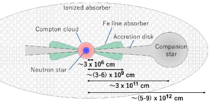
Figure 5: Schematic view of Swift J1858.6$-$0814 in the case of an ionized absorber covering the entire binary system See the text in detail.

Based on these values, we show a schematic view of the system in figure 5 in the case of ionized absorber covering the entire binary system. The Compton cloud completely covers the emission region, that is, the blackbody radiation from the NS. The size of the Compton cloud is assumed to extend to the inner radius of the accretion disk. The highly-ionized gas from the inner accretion disk would be producing an ionized iron absorption line.

6 Summary

We analyzed NICER archive data of the transient NS-LMXB Swift J1858.6$-$0814. The average spectrum was reproduced with a blackbody emission ($kT_{\rm bb}$ = 1.1 keV) comptonized with an optically-thick gas (”Compton cloud”; $kT_{\rm e}\sim 10$ keV and $\tau\sim 5$) and the multi-temperature blackbody emission ($kT_{\rm in}\sim 0.7$ keV) combined with three emission lines and an absorption line. The two emission lines were identified as highly ionized atoms Ne, whereas the one was consistent with neutral-like Fe. The highly ionized absorption line of Fe was detected. These observations support the existence of the highly-ionized gas in the inner accretion disk in Swift J1858.6$-$0814.

References

- Arnaud (1996) Arnaud, K. A. 1996, Astronomical Data Analysis Software and Systems V, 101, 17
- Boirin et al. (2004) Boirin, L., Parmar, A. N., Barret, D., Paltani, S. & Grindlay, J. E. 2004, A&A, 418, 1061
- Buisson et al. (2020a) Buisson, D. J. K., et al. 2020a, MNRAS, 498, 68
- Buisson et al. (2020b) Buisson, D. J. K., et al. 2020b, MNRAS, 499, 793
- Buisson et al. (2021) Buisson, D. J. K., et al. 2021, MNRAS, 503, 5600
- Díaz Trigo and Boirin (2016) Díaz Trigo, M. & Boirin, L. 2016, Astronomische Nachrichten, 337, 368
- Done et al. (2018) Done, C., Tomaru, R., & Takahashi, T. 2018, MNRAS, 473, 838
- Gendreau et al. (2016) Gendreau, K. C., et al. 2016, Proc. SPIE, 9905, 99051H
- Kallman & Bautista (2001) Kallman, T. & Bautista, M. 2001, ApJS, 133, 221
- Knight et al. (2022) Knight, A. H., Ingram, A., & Middleton, M. 2022, MNRAS, 514, 1908
- Kotani et al. (2000) Kotani, T., Ebisawa, K., Dotani, T., Inoue, H., Nagase, F., Tanaka, Y., & Ueda, Y. 2000, ApJ, 539, 413
- Kotani et al. (2006) Kotani, T., Ebisawa, K., Dotani, T., Inoue, H., Nagase, F., Tanaka, Y., & Ueda, Y. 2006, ApJ, 651, 615
- Krimm et al. (2018) Krimm, H. A. et al. 2018, The Astronomer’s Telegram, 12151
- Matsuoka et al. (2009) Matsuoka, M., et al.2009, PASJ, 61, 999
- Mihara et al. (2011) Mihara, T., et al. 2011, PASJ, 63, S623
- Mitsuda et al. (1984) Mitsuda, K., et al. 1984, PASJ, 36, 741
- Sugizaki et al. (2011) Sugizaki, M., et al. 2011, PASJ, 63, S635
- Ueda et al. (2004) Ueda, Y., Murakami, H., Yamaoka, K., Dotani,T., & Ebisawa, K. 2004, ApJ, 609, 325
- Ulrich et al. (1999) Ulrich, M.-H., Comastri, A., Komossa, S., & Crane, P. 1999, A&A, 350, 816
- Wang et al. (2021) Wang, J., et al. 2021, ApJ, 910, L3
- Wilms et al. (2000) Wilms, J., Allen, A., & McCray, R. 2000, ApJ, 542, 914
- Zdziarski et al. (1996) Zdziarski, A. A., Johnson, W. N., & Magdziarz, P. 1996, MNRAS, 283, 193
- Zdziarski et al. (2020) Zdziarski, A. A., Szanecki, M., Poutanen, J., Gierliński, M., & Biernacki, P. 2020, MNRAS, 492, 5234