Multiple Locally Linear Kernel Machines

Abstract

In this paper we propose a new non-linear classifier based on a combination of locally linear classifiers. A well known optimization formulation is given as we cast the problem in a $\ell_{1}$ Multiple Kernel Learning (MKL) problem using many locally linear kernels. Since the number of such kernels is huge, we provide a scalable generic MKL training algorithm handling streaming kernels. With respect to the inference time, the resulting classifier fits the gap between high accuracy but slow non-linear classifiers (such as classical MKL) and fast but low accuracy linear classifiers.

1 Introduction

SVMs were shown to provide very accurate classifiers, and are consequently used in a growing number of applications. SVM training algorithms and subsequent inference efficiency can be separated in two groups, depending on the kernel being linear or not. When dealing with linear SVMs, very efficient training algorithms based on stochastic gradient descent such as (shalevshwartz07icml; bordes09jmlr; leroux12nips) allow to deal with large datasets in a short amount of time. The inference time of linear SVMs is clearly their main advantage as it can efficiently be optimized for modern computer architecture. However, many classification problems are not linearly separable and consequently a non linear kernel is required.

Kernel SVMs also benefit from recent developments in stochastic coordinate methods such as (bordes05jmlr; shalevshwartz13jmlr; shalevshwartz14icml) and come now with efficient training procedures. The main drawback of Kernel SVMs is the inference time which is proportional to the number of support vectors. This number has been experimentally shown to grow linearly with the size of the training set (bordes05jmlr). Most of the speed-up is obtained by limiting the number of support vector (dekel06nips). For example, in (ertekin11pami), the authors proposed to ignore outliers to reduce the number of support vectors, but the problem becomes non-convex and the resulting classifier still has a high inference time.

With respect to the inference cost, a much more efficient alternative is the use of almost linear classifiers such as Locally Linear SVM (LLSVM) proposed in (ladicky11icml). In LLSVM, a generative manifold learning algorithm produces a partition the input space. An almost piece-wise linear classifier concatenating linear classifier of the different parts is then trained. The inference cost of LLSVM is almost as fast as for linear SVMs, depending only on the number of anchor points used in the manifold learning. However, LLSVMs are dependent on the success of the manifold learning algorithm that provides the anchor points. Moreover, the parameter tuning of such algorithms, mainly the number of anchor points and the coding function, is often costly and difficult to perform.

In this paper, we propose a new locally linear classifier similar to LLSVM, but without the burden of the manifold learning part while keeping very efficient inference procedure. We first define a family of locally linear kernels which are related to conformal kernels (amari99nn). We then used the Multiple Kernel Learning (MKL) framework (bach04icml) to select a subset of the locally linear kernels. The $\ell_{1}$-norm constraint on the kernel combination leads to a limited number of selected kernels and consequently leads to low inference cost. Our contributions can be summed up as the following: 1) we propose a new learning problem named Multiple Locally Linear Kernel Machine (MLLKM) to obtain locally linear classifiers more easily. 2) Since MLLKM is similar to $\ell_{1}$-MKL, we propose a new $\ell_{1}$-MKL solver that can handle the high number of kernels in MLLKM.

The remaining of this paper is organized as follows. In the next section, we review existing works on locally linear classifiers. In Section 3, we detail the concept of locally linear kernels. Then, we present our proposed MLLKM problem and show it is equivalent to solving $\ell_{1}$-MKL. In the same section, we present a fast algorithm to solve $\ell_{1}$-MKL problems on a budget and show several strategies to automatically tune the parameters and drastically lower the number of selected kernels. We present experiments in Section LABEL:sec:exp before we conclude.

2 Locally Linear Classifiers

Generally, a locality criterion in machine learning refers to an adaptation of the model with respect to the localization in the input space. For instance, the idea of locally linear classification is to consider a combination of different linear predictors depending on some locality criterion performed on the evaluated sample. Remark that although the predictors are linear, the combination might not, and consequently the resulting classifier can perform non-linear separation.

In Locally Linear SVM (ladicky11icml), a dictionary learning algorithm is used to provide a set of anchor points $\{\mathbf{x}_{c}\}$ that describe the manifold of the data. This set is usually obtained using a k-means clustering of a large set of (unlabeled) samples, although more sophisticated method can be used. Any sample $\mathbf{x}$ can then be coded by the anchor points $\mathbf{x}_{c}$ using local coordinate $\gamma_{\mathbf{x}_{c}}(\mathbf{x})$ such that $\sum_{\mathbf{x}_{c}}\gamma_{\mathbf{x}_{c}}(\mathbf{x})=1$ and $\mathbf{x}\approx\sum_{\mathbf{x}_{c}}\gamma_{\mathbf{x}_{c}}(\mathbf{x})\mathbf{x}_{c}$ (yu09nips). Examples of such local coordinate coding include Kernel Codebook (gemert08eccv) and Locality constraint Linear Coding (wang10cvpr). These local coordinate are then used to perform the combination of local classifiers:

$$f(\mathbf{x})=\gamma_{\mathbf{x}_{c}}(\mathbf{x})^{\top}\mathbf{W}\mathbf{x}+\gamma_{\mathbf{x}_{c}}(\mathbf{x})^{\top}\mathbf{b},$$

with $\mathbf{W}$ being the matrix which lines are the local hyperplanes and $\mathbf{b}$ is a vector of local biases. To train $\mathbf{W}$ and $\mathbf{b}$, very efficient stochastic gradient descent algorithms can be used on each local hyperplane weighted by the local coordinate. Extension to multiclass problems can be achieve by replacing the hinge loss with a multiclass loss as presented in (fornoni13acml).

In (gonen08icml), the authors proposed to tackle the localization as a multiple kernel learning problem, using quasi-conformal transformation:

$$K_{\eta}(\mathbf{x}_{i},\mathbf{x}_{j})=\sum_{m}\eta_{m}(\mathbf{x}_{i})\eta_{m}(\mathbf{x}_{j})K_{m}(\mathbf{x}_{i},\mathbf{x}_{j}),$$

where $\eta_{m}(\cdot)$ is a locality function that aims at selecting the right kernel among the $K_{m}$ depending on $\mathbf{x}_{i}$ and $\mathbf{x}_{j}$. As in LLSVM, the authors proposed each locality function $\eta_{m}$ to be associated with an anchor point $\mathbf{v}_{m}$:

$$\eta_{m}(\mathbf{x})=\frac{exp(\langle\mathbf{v}_{m},\mathbf{x}\rangle+v_{m0})}{\sum_{k}exp(\langle\mathbf{v}_{k},\mathbf{x}\rangle+v_{ik0})}$$

The resulting MKL problem has then 2 sets of variables, namely the dual SVM variables $\alpha$ associated with the training samples, and the anchor points $\mathbf{v}_{m}$ that define the kernels in the combination. The LMKL algorithm consists in an alternate optimization scheme between $\alpha$ and $\mathbf{v}_{m}$, where the $\mathbf{v}_{m}$ are optimized using a gradient descent strategy. In case of linear kernels, it is easy to see LLSVM and LMKL lead to the same family of classifiers, with LMKL allowing to tune the anchor points to the specific classification task. However, since the LMKL objective function is non-convex, a local optimum is found.

Both methods rely on a manifold learning procedure to determine the anchor points. The main problem of such method is that it often leads to a non-convex problem for which no guarantee on the solution can be given, and that is likely to have a high computational cost. Moreover, the parameter tuning of such solution (i.e., the number of anchor points, the coding functions) is very difficult to perform. In practice, it relies on an exploration of the parameters space using cross-validation which is very costly.

In this paper, we thus propose to remove the burden of the manifold learning part by casting the selection of the anchor points and the parameters in a MKL problem. To be able to do that, we first define a family of locally linear kernels in the next section.

3 Locally linear kernels

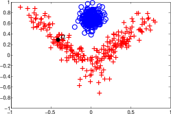
(a) Original space $\mathbb{R}^{2}$

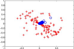
(b) Gaussian map

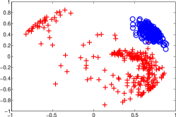
(c) Exponential map

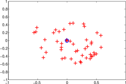
(d) Linear map

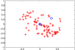
(e) Squared map

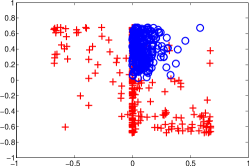
(f) Component wise Gaussian map

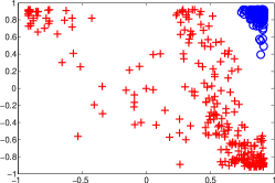
(g) Component wise exponential map

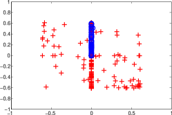
(h) Component wise linear map

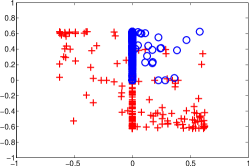
(i) Component wise squared map

Figure 1: Example of synthetic data and corresponding $\mathcal{X}_{c}$ for different types of maps, with anchor point $a$.

Let $\mathbf{x}_{1},\mathbf{x}_{2}\in\mathbb{R}^{d}$ be two element of $\mathbb{R}^{d}$, and $\langle\mathbf{x}_{1},\mathbf{x}_{2}\rangle=\mathbf{x}_{1}^{\top}\mathbf{x}_{2}$ the standard dot product . Let the norm $\|\mathbf{x}\|=\sqrt{\langle\mathbf{x},\mathbf{x}\rangle}$ and the metric $d(\mathbf{x}_{1},\mathbf{x}_{2})=\|\mathbf{x}_{1}-\mathbf{x}_{2}\|$ be the standard (euclidean) norm and metric associated with $\langle\cdot,\cdot\rangle$.

We propose to explicitly build a Hilbert space $\mathcal{X}_{c}$ as a subspace of the input space $\mathbb{R}^{d}$ locally defined around an arbitrarily chosen center $\mathbf{x}_{c}\in\mathbb{R}^{d}$. To enforce locality, we center the data on $\mathbf{x}_{c}$ and then apply a norm scaling function that tends to map the vectors to $0$ when the norm becomes to large. The mapping from $\mathbb{R}^{d}$ to $\mathcal{X}_{c}$ has the following expression:

$$\phi_{c}: \mathbb{R}^{d}\rightarrow\mathcal{X}$$ (1)

$$\mathbf{x}\mapsto h^{(c)}(\mathbf{x})(\mathbf{x}-\mathbf{x}_{c})$$

Where $h^{(c)}$ is a conformal map rendering the vicinity of the given center $\mathbf{x}_{c}$. We show in Table 1 several examples of such mappings.

Table 1: Examples of conformal maps used in this work, with $|t|_{+}=\max(0,t)$.

name	definition	bounded	smooth
$h_{e}^{(c)(\mathbf{x})}$	$e^{-\gamma\|\mathbf{x}-\mathbf{x}_{c}\|}$	-	-
$h_{g}^{(c)}(\mathbf{x})$	$e^{-\gamma\|\mathbf{x}-\mathbf{x}_{c}\|^{2}}$	-	$\checkmark$
$h_{l}^{(c)}(\mathbf{x})$	$\left|1-\gamma\|\mathbf{x}-\mathbf{x}_{c}\|\right|_{+}$	$\checkmark$	-
$h_{s}^{(c)}(\mathbf{x})$	$\left|1-\gamma\|\mathbf{x}-\mathbf{x}_{c}\|^{2}\right|_{+}$	$\checkmark$	$\checkmark$

By definition, $\mathcal{X}_{c}$ is a Hilbert space endowed with the following explicit dot product $k_{c}(\cdot,\cdot)$:

$$k_{c}(\mathbf{x}_{1},\mathbf{x}_{2})= \langle\phi_{c}(\mathbf{x}_{1}),\phi_{c}(\mathbf{x}_{2})\rangle_{\mathcal{X}_{c}}$$

$$= \left(h^{(c)}(\mathbf{x}_{1})(\mathbf{x}_{1}-\mathbf{x}_{c})\right)^{\top}\left(h^{(c)}(\mathbf{x}_{2})(\mathbf{x}_{2}-\mathbf{x}_{c})\right)$$

The properties of $\mathcal{X}_{c}$ depends on the family of mappings $h$ chosen, which we consider to be a hyperparameter, and its subsequent parameters, namely $\{\gamma,\mathbf{x}_{c}\}$ in our examples. We show in Figure 1 examples of such mapping on synthetic data. As we can see, many samples are mapped to or close to 0. The effect is all the more visible using bounded maps, since samples outside of the support of $\phi_{c}$ are mapped exactly to 0. However, the local geometry of the point cloud is preserved.

To allow for more sophisticated manipulations, we also consider component wise local mappings, in the form of:

$$\phi_{c}: \mathbb{R}^{d}\rightarrow\mathcal{X}$$ (2)

$$\mathbf{x}\mapsto\mathbf{h}^{(c)}(\mathbf{x})\circ(\mathbf{x}-\mathbf{x}_{c})$$

where $\circ$ is the entry wise (Hadamard) product. With a slight abuse of notations, the mapping $\mathbf{h}:\mathbb{R}^{d}\mapsto\mathbb{R}^{d}$ now produces a vector rendering the vicinity of each component to the anchor point. The explicit dot product corresponding to $\mathcal{X}_{c}$ is then the following:

$$k_{c}(\mathbf{x}_{1},\mathbf{x}_{2})=\\ \left(h^{(c)}(\mathbf{x}_{1})\circ(\mathbf{x}_{1}-\mathbf{x}_{c})\right)^{\top}\left(h^{(c)}(\mathbf{x}_{2})\circ(\mathbf{x}_{2}-\mathbf{x}_{c})\right)$$

Using the examples given in Table 1 on each component of input samples $\mathbf{x}$ produces the corresponding component wise mappings. These mappings are also illustrated in Figure 1.

The main difference between the global and the component wise mappings is that the latter makes the assumption the components can be considered independently, which is the case if the features have been decorrelated (e.g., after a Karhunen-Loève transform).

It is clear that using only one of such kernels (either global or component wise) has less discriminatory capabilities than the simple linear kernel. Indeed, since many features are mapped to 0 independently of their class, it is very likely that the classification problem becomes non linearly separable after the transform. We thus consider the case where several locally linear kernels are used and summed into a single kernel:

$$k(\mathbf{x}_{1},\mathbf{x}_{2})=\sum_{c}k_{c}(\mathbf{x}_{1},\mathbf{x}_{2})$$ (3)

The resulting space $\mathcal{X}$ is the concatenation of the $\mathcal{X}_{c}$. Problems that were not linearly separable in $\mathbb{R}^{d}$ (for example the synthetic data of Figure 1) can be in $\mathcal{X}$, provided a sufficient number of locally linear kernels with the right range of locality are used.

To choose these kernels, we consider the training set $\mathcal{A}$ of samples $\{\mathbf{x}_{i}\}_{i}$ of $\mathbb{R}^{d}$ to be used to train the classifier. We propose to perform a linear combination consisting of a locally linear kernel for each sample:

$$k(\mathbf{x}_{1},\mathbf{x}_{2})=\sum_{\mathbf{x}_{c}\in\mathcal{A}}\beta_{c}k_{c}(\mathbf{x}_{1},\mathbf{x}_{2})$$ (4)

We are now left with the optimization of $\beta$ so as to discard irrelevant kernels from the combination. The next section devises the resulting optimization problem and proposes an algorithm to solve it.

4 Multiple Locally Linear Kernel Machines

Let $\mathcal{A}=\{(\mathbf{x}_{i},y_{i})\}_{1\leq i\leq n}$ be a training set of $n$ training samples $\mathbf{x}_{i}\in\mathbb{R}^{d}$ and their associated labels $y_{i}\in\{-1,1\}$. The Multiple Locally Linear Kernel Machine (MLLKM) is then the optimal predictor according to the following primal problem:

$$\min_{w,\beta,\zeta} \frac{1}{2}\sum_{m=1}^{n}\|w_{m}\|_{\mathcal{H}_{m}}^{2}+C\sum_{i=1}^{n}\zeta_{i}$$ (5)

$$s.t. \forall i,y_{i}\sum_{m}\sqrt{\beta_{m}}w_{m}^{\top}\phi_{m}(\mathbf{x}_{i})\geq 1-\zeta_{i}$$

$$\forall i,\zeta_{i}\geq 0$$

$$\forall m,\beta_{m}\geq 0$$

$$\sum_{m}\beta_{m}=1$$

Remark this is corresponds to a standard $\ell_{1}$-constraint MKL problem with the slight difference that the number of kernels is the same as the number of training samples. On many occasions, $\ell_{p}$-MKL with $p>1$ are known to perform better than $\ell_{1}$ constraint (kloft09nips), however the number of kernels in MLLKM is too high to allow for non sparse combinations. In such case, the computational benefit of having a locally linear classifier would be lost to the very high number of linear predictors in the resulting combination.

To recover classical formulation of $\ell_{1}$-MKL, we consider the following Lagrangian of the primal problem with $\beta$ left in the constraints:

$$\mathcal{L}(w,\beta,\zeta,\alpha,\lambda) =\frac{1}{2}\sum_{m}\|w_{m}\|^{2}+\sum_{i}\left(C-\lambda_{i}-\alpha_{i}\right)\zeta_{i}$$

$$-\sum_{i}\alpha_{i}\left[y_{i}\sum_{m}\sqrt{\beta_{m}}w_{m}^{\top}\phi_{m}(\mathbf{x}_{i})-1\right]$$

$$s.t. \quad\forall m,\beta_{m}\geq 0$$

$$\quad\sum_{m}\beta_{m}=1$$

The KKT stationary condition on $w$ states that:

$$\frac{\partial\mathcal{L}}{\partial w_{m}^{\star}}=0=w_{m}^{\star}-\sum_{i}\alpha_{i}y_{i}\sqrt{\beta_{m}^{\star}}\phi_{m}(\mathbf{x}_{i})$$

Or equivalently:

$$w_{m}^{\star}=\sum_{i}\alpha_{i}y_{i}\sqrt{\beta_{m}^{\star}}\phi_{m}(\mathbf{x}_{i})$$

Similarly, the stationary condition on $\zeta$ states that:

$$\frac{\partial\mathcal{L}}{\partial\zeta_{i}}=0=C-\alpha_{i}-\lambda_{i}$$

Since $\alpha$ and $\lambda$ are dual variables, the dual feasibility condition imposes their positiveness, and in particular implies a box constraint on $\alpha$:

$$\forall i,0\leq\alpha_{i}\leq C$$

A dual formulation of problem (5) for $w$ and $\zeta$ variables is then obtained by injecting these conditions into the original formulation:

$$\mathcal{D}(\alpha,\beta) =\inf_{w,\zeta}\mathcal{L}(w,\beta,\zeta,\alpha,\lambda)$$

$$=\sum_{i}\alpha_{i}-\frac{1}{2}\sum_{i,j}\alpha_{i}\alpha_{j}y_{i}y_{j}\sum_{m}\beta_{m}k_{m}(\mathbf{x}_{i},\mathbf{x}_{j})$$

$$s.t. \quad\forall m,\beta_{m}\geq 0$$

$$\quad\sum_{m}\beta_{m}=1$$

This dual expression allows us to recover to the well known $\min\max$ formulation used for example in (rakoto08jmlr):

$$\min_{\beta}\max_{\alpha} \sum_{i}\alpha_{i}-\frac{1}{2}\sum_{i,j}\alpha_{i}\alpha_{j}y_{i}y_{j}\sum_{m}\beta_{m}k_{m}(\mathbf{x}_{i},\mathbf{x}_{j})$$ (6)

$$s.t. \quad\forall i,0\leq\alpha_{i}\leq C$$

$$\quad\forall m,\beta_{m}\geq 0$$

$$\quad\sum_{m}\beta_{m}=1$$

Since the number of kernels is equal to the number of training samples, large datasets lead to optimization problem intractable for current algorithms. In particular, most algorithms suppose all kernel matrices can be computed and stored in memory beforehand, which is clearly not the case when considering even medium sized datasets (i.e., more than 10k samples). Consequently, we present a new algorithm called SequentialMKL, for solving large MKL problems with reduced memory footprint that is suitable for training MLLKM.

4.1 Sequential MKL

The main idea in SequentialMKL is to consider a reduced active set of kernels, solve the MKL problem for this reduced set, and then probe new kernels for inclusion in the set. Solving the MKL problem with a reduced set of active kernels can be done efficiently using existing solver like (sonnenburg06jmlr; chapelle08nipsw) or (rakoto08jmlr). In our case, we choose the reduced gradient approach of SimpleMKL of (rakoto08jmlr) since it is closely related to the inclusion criterion of new kernels. For the internal SVM solver, we use a variant of SDCA (shalevshwartz13jmlr) presented in Algorithm 1. We keep track of the outputs $\hat{\mathbf{y}}$ of the classifier and check for an early bail out criterion to improve the cost of each iteration.

Algorithm 1 SDCA for solving SVM

SDCA$\mathbf{y}$, $K$, $E$, $C$$\hat{\mathbf{y}}\leftarrow\bf 0$, $\alpha\leftarrow\bf 0$, $e\leftarrow 0$$L\leftarrow$random permutation of $\{1,...,n\}$$i\in L$$g\leftarrow 1-\mathbf{y}_{i}\hat{\mathbf{y}}_{i}$$g=0$or ($g>0$ and $\alpha_{i}=C$) or ($g<0$ and $\alpha_{i}=0$)          skip $i$$\alpha_{new}\leftarrow\max(0,\min(\alpha_{i}+g/K_{ii},C))$$\delta\leftarrow\alpha_{new}-\alpha_{i}$$j\in\{i,...,n\}$$\hat{\mathbf{y}}_{j}\leftarrow\hat{\mathbf{y}}_{j}+\delta\mathbf{y}_{j}K_{ij}$$e\leftarrow e+1$$e\geq E$$\alpha$

To design the criterion for inserting new kernels to the active set, we consider a Lagrangian of the $\min\max$ problem 6 where the constraints of $\beta$ are taken into account:

$$\mathcal{M}(\alpha,\beta,\mu,\nu)=\sum_{i}\alpha_{i}-\sum_{m}\mu_{m}\beta_{m}-\nu\left(\sum_{m}\beta_{m}-1\right)\\ -\frac{1}{2}\sum_{i,j}\alpha_{i}\alpha_{j}y_{i}y_{j}\sum_{m}\beta_{m}k_{m}(\mathbf{x}_{i},\mathbf{x}_{j})$$

Now, the stationary condition at optimum $\beta^{\star}$ imposes that

$$\nu^{\star}=-\mu_{m}^{\star}-\frac{1}{2}\sum_{i,j}\alpha_{i}^{\star}\alpha_{j}^{\star}y_{i}y_{j}k_{m}(\mathbf{x}_{i},\mathbf{x}_{j})$$

Or, equivalently $\forall m,\forall l$:

$$\mu_{m}^{\star}+\frac{1}{2}\sum_{i,j}\alpha_{i}^{\star}\alpha_{j}^{\star}y_{i}y_{j}k_{m}(\mathbf{x}_{i},\mathbf{x}_{j})=\\ \mu_{l}^{\star}+\frac{1}{2}\sum_{i,j}\alpha_{i}^{\star}\alpha_{j}^{\star}y_{i}y_{j}k_{l}(\mathbf{x}_{i},\mathbf{x}_{j})$$

Let us denote $k_{k}$ a kernel with non-zero weight $\beta_{k}^{\star}$ at optimum, then $\mu_{k}^{\star}=0$ by complementary slackness. In turns, it means that $\forall l\neq k$,

$$\frac{1}{2}\sum_{i,j}\alpha_{i}^{\star}\alpha_{j}^{\star}y_{i}y_{j}k_{k}(\mathbf{x}_{i},\mathbf{x}_{j})= \mu_{l}+\frac{1}{2}\sum_{i,j}\alpha_{i}^{\star}\alpha_{j}^{\star}y_{i}y_{j}k_{l}(\mathbf{x}_{i},\mathbf{x}_{j})$$

$$\geq \frac{1}{2}\sum_{i,j}\alpha_{i}^{\star}\alpha_{j}^{\star}y_{i}y_{j}k_{l}(\mathbf{x}_{i},\mathbf{x}_{j})$$ (7)

since by dual feasibility all $\mu_{l}^{\star}\geq 0$. The criterion thus consists in finding a kernel of the open kernel set violating constraint (4.1) and adding it to the current active kernel set. For numerical stability reasons, we compute the largest $\frac{1}{2}\sum_{i,j}\alpha_{i}\alpha_{j}y_{i}y_{j}k_{m}(\mathbf{x}_{i},\mathbf{x}_{j})$ among non zero weight kernels $k_{m}$. Remark that kernels respecting Equation (4.1) have zero weight and $\mu_{m}$ equals to the difference of gradients with $k_{k}$, meaning the KKT conditions are respected.

The full SequentialMKL algorithm is presented in Algorithm LABEL:alg:smkl. We alternate between optimizing the kernel weights and search for new kernel to insert in the active set, until no new kernel can be inserted.

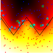
(a) Gaussian map

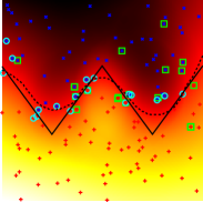
(b) Square map

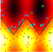
(c) Component Gaussian map

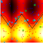
(d) Component Square map

Figure 2: Example of synthetic data classification task. The true boundary is shown in plain black line, while the classifier boundary is in dashed black line. The circles denote the support vectors, while the squares denote the support kernels.

Algorithm 2 SequentialMKL

train$\{k_{m}\}$, $\mathbf{x}$, $\mathbf{y}$, $E$, $C$$\mathcal{S}\leftarrow k_{1}$, $\mathcal{O}\leftarrow\{k_{m}\}\backslash k_{1}$$\beta\leftarrow\bf 1$, $\alpha\leftarrow\bf 0$$K\leftarrow\sum_{k_{m}\in\mathcal{S}}\beta_{m}k_{m}$$\alpha\leftarrow$SDCA($\mathbf{y}$, $K$, $E$, $C$) $term\leftarrow\bf true$$g\leftarrow\max_{k_{m}\in\mathcal{S}}\frac{1}{2}\sum_{i,j}\alpha_{i}\alpha_{j}y_{i}y_{j}k_{m}(i,j)$$k_{m}\in\mathcal{O}$$\frac{1}{2}\sum_{i,j}\alpha_{i}\alpha_{j}y_{i}y_{j}k_{m}(i,j)>g$$term\leftarrow\bf false$$\mathcal{S}\leftarrow\mathcal{S}+k_{m}$, $\mathcal{O}\leftarrow\mathcal{O}\backslash k_{m}$$\beta\leftarrow$SolveMKL($\mathcal{S}$,