Asymptotic online FWER control for dependent test statistics

Abstract

In online multiple testing, an a priori unknown number of hypotheses are tested sequentially, i.e. at each time point a test decision for the current hypothesis has to be made using only the data available so far. Although many powerful test procedures have been developed for online error control in recent years, most of them are designed solely for independent or at most locally dependent test statistics. In this work, we provide a new framework for deriving online multiple test procedures which ensure asymptotical (with respect to the sample size) control of the familywise error rate (FWER), regardless of the dependence structure between test statistics. In this context, we give a few concrete examples of such test procedures and discuss their properties. Furthermore, we conduct a simulation study in which the type I error control of these test procedures is also confirmed for a finite sample size and a gain in power is indicated.

Keywords asymptotics  $\cdot$ dependent test statistics  $\cdot$ familywise error rate  $\cdot$ online multiple testing

1 Introduction

In times when ever larger amounts of data become more readily available, there is a growing interest in being able to carry out numerous statistical tests as quickly as possible. To this end, the online setting that was introduced by Foster and Stine in [8], provides a flexible framework, where it is assumed that an unknown and arbitrary large number of hypotheses can be tested in a sequential manner. In order to address the arising multiplicity problems, many different online test procedures have been developed over the years. While most of them aim for the control of the false discovery rate [8, 1, 9, 12], there are also situations, in which the control of the familywise error rate (FWER) may be more appropriate. This can be the case, when optimizing machine learning algorithms [4] or in a platform trial, where different treatment arms start at different time points and use a shared control group [14]. In [17] Tian and Ramdas developed online procedures specifically for FWER control, e.g. the powerful ADDIS-Spending algorithm. Furthermore, Fischer et al. derived an online version of the traditional closure principle in [5] and in [6] another powerful procedure was proposed, the so called ADDIS-Graph.

Despite the great progress in the online literature over the recent years, there is still a lack of methods, that work for dependent test statistics or $p$-values, as it was for example also recently addressed in [13]. However, in reality it is often way more plausible that there are certain underlying dependencies. As a concrete motivational example, consider the case of a platform trial (see Figure 1). Here, dependency issues arise due to the shared control data. Online algorithms for error control in platform trials have been considered e.g. in [14] and [18]. But there are also other reasons why observations corresponding to different hypotheses could be highly dependent. For example, the observations regarding different hypotheses could originate from the same individual or a hypothesis that was not rejected at first could be tested again using old and new data. Another application that causes dependencies, would be public databases, where different independent research groups have access to the same data and perform their own tests and analyses [13].

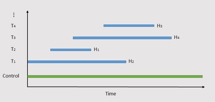
Figure 1: Diagram of a platform trial

In the literature so far, the test levels of online procedures depend only on the previous $p$-values or discrete transformations of them [9, 12, 17]. When $p$-values are dependent, it is no longer possible to use them directly for specifying test levels. In [19] Zrnic et al. circumvented this issue by using only the information of $p$-values that are guaranteed to be independent from the current one, which requires some knowledge of the dependency structure. In this paper we propose a flexible method, that uses the data (instead of just the $p$-value) and can be equally applied, even when there are dependencies in the data and no or few information of the exact dependency structure is available. Thereby we make use of a resampling method that is known as the low intensity bootstrap (also referred to as $m$ out of $n$ bootstrap) originally proposed in [16] and thoroughly discussed in [2]. This is a resampling strategy, where resampling is done with a lower sample size ($m$ instead of $n$) than in the original sample. It can be shown, that in some cases this leads to consistency, even when the traditional bootstrap fails [2].

The remainder of the paper is structured as follows: In Section 2 we introduce the underlying set-up and notation and review some of the already existing methods for online familywise error rate control. The main results are given in Section 3, where we introduce the notion of consistent weights and, building upon this, derive new online procedures for FWER control under dependency. In Section 4 numerical simulations are performed in two different settings to exemplify the theoretical considerations. The results are again summarized and discussed in Section 5. The more technical proofs and derivations are given in the Appendix.

2 Preliminaries

2.1 Notation and model set-up

Suppose we want to sequentially test null hypotheses $H_{1},H_{2},H_{3},\dots$ and at each step $i$ we perform the test based on data $\mathcal{X}_{i}$, generated by the true distribution $\mathbb{P}$. In each case, the corresponding sample size, denoted by $n_{i}$, is assumed to be data independent. Note that we make no further assumptions on the data sets, so they possibly could have an arbitrary overlap for different hypotheses or even coincide. With $n\in\mathbb{N}$ we denote a general parameter of the sample size, i.e. for all $i\in\mathbb{N}$ it holds that $n_{i}\rightarrow\infty$ as $n\rightarrow\infty$. All asymptotic considerations throughout this paper are performed by letting $n\rightarrow\infty$. When testing the null hypothesis $H_{i}$ versus the alternative $H^{\prime}_{i}$ the decisions are made in terms of test statistics $T_{i,n}(\mathcal{X}_{i})$ or $p$-values $P_{i,n}(\mathcal{X}_{i})$. The latter is more in line with the common assumption in the online multiple testing literature. An online test procedure is then a family of test levels $(\alpha_{i,n})_{i\in\mathbb{N}}$ that depend on the previous data, i.e. $\alpha_{i,n}=\alpha_{i,n}(\mathcal{X}_{1},\dots,\mathcal{X}_{i-1})$. We will not use the more general mathematical definition of an online multiple test suggested in [5].
For an $N\in\mathbb{N}$ let further denote the set of indices corresponding to the true null hypotheses among $H_{1},\dots,H_{N}$ by $\mathcal{H}^{0}=\mathcal{H}^{0}(N)$ and the number of erroneously rejected hypotheses by $V_{n}=V_{n}(N)=\sum_{i\in\mathcal{H}^{0}}\mathds{1}\{P_{i,n}\leq\alpha_{i,n}\}$. Then, the familywise error rate is defined as

$$\mathrm{FWER}_{n}=\mathrm{FWER}_{n}(N)=\mathbb{P}(V_{n}\geq 1).$$

The goal is to derive online test procedures that control the familywise error rate asymptotically, i.e. for any $N\in\mathbb{N}$ it holds that

$$\limsup_{n\rightarrow\infty}\mathrm{FWER}_{n}(N)\leq\alpha.$$ (1)

Equation (1) says that the familywise error rate is controlled asymptotically (with respect to the sample size) for any finite number of hypotheses $N$. In contrast to the case of exact error control, where this would also imply the statement for an infinite number of hypotheses, we can not guarantee that

$$\limsup_{n\rightarrow\infty}\limsup_{N\to\infty}\mathrm{FWER}_{n}(N)\leq\alpha$$

will hold. For this, further assumptions regarding uniform convergence among all hypotheses might be needed, which are not realistic in this general hypothesis testing set-up. Moreover, (1) reflects the common situation found in essentially all real life applications, where the number of hypotheses is a priori unknown but finite.

2.2 Existing procedures for online FWER control

We start reviewing some of the currently existing procedures for online FWER control. The most straight forward method is the so called Alpha-Spending algorithm [8]. The idea is to simply divide the global error budget among all hypotheses and thus it can be seen as an online version of the weighted Bonferroni correction in traditional multiple testing. This can be implemented by selecting a non-negative sequence $(\alpha_{i})_{i\in\mathbb{N}}$ such that

$$\sum_{i\in\mathbb{N}}\alpha_{i}=\alpha.$$

It can easily be shown by the Bonferroni inequality that this procedure controls the familywise error rate regardless of the dependence structure of the $p$-values. Unfortunately, it is generally conservative, so there is an interest in developing new and more powerful online multiple testing procedures.

In [17] Tian and Ramdas derived advanced spending algorithms, first and foremost the powerful ADDIS-Spending procedure, which combines the concepts of adaptivity and discarding. Since we focus in this work on the notion of adaptivity (see also the discussion in Section 5), i.e. accounting for the proportion of true null hypotheses, we briefly introduce the so called Adaptive-Spending [17]. For this, let $\lambda\in(0,1)$ and $(\gamma_{i})_{i\in\mathbb{N}}$ be a non-negative sequence such that $\sum_{i\in\mathbb{N}}\gamma_{i}=1$. Furthermore, we define the so called candidate indicator of the $i$-th $p$-value by $C_{i}=\mathds{1}\{P_{i}\leq\lambda\}$. Tian and Ramdas showed that, as long as the $p$-values are independent, it is sufficient for FWER control that the online procedure $(\alpha_{i})_{i\in\mathbb{N}}$ satisfies

$$\sum_{i\in\mathbb{N}}\frac{1-C_{i}}{1-\lambda}\alpha_{i}\leq\alpha.$$ (2)

As a concrete example, they proposed the procedure given by

$$\alpha_{i}=\alpha\cdot(1-\lambda)\cdot\gamma_{t(i)},$$ (3)

where $t(i)=1+\sum_{j<i}(1-C_{j})$.

The idea of (2) is to decrease the remaining error budget only when a true null hypothesis has been tested. The use of the candidate indicator, as surrogate for the indicator of a true alternative, relies on the fact that $p$-values corresponding to true alternatives are usually small and therefore rather unlikely exceed the threshold $\lambda$. The factor $(1-\lambda)$ accounts for the $p$-values, for which the null hypothesis is true (from now on referred to as null $p$-values), that are by chance smaller than $\lambda$.

Since the test levels in (3) directly depend on the previous $p$-values, we need the underlying assumption that the null $p$-values are valid conditional to the previous $p$-values, i.e. for all $i\in\mathcal{H}^{0}$ and $x\in[0,1]$ it holds that

$$\mathbb{P}(P_{i}\leq x|P_{1},\dots,P_{i-1})\leq x.$$ (4)

By using the same proof as in [17], it is clear that FWER control is guaranteed when (2) and (4) are fulfilled. While (4) is always true when the $p$-values are independent, it is easily violated when dependencies between the $p$-values are present as demonstrated in the following example.

Example 2.1.

Let $(Z_{1},Z_{2})$ be bivariate normally distributed with means $\mathbb{E}(Z_{1})=\mathbb{E}(Z_{2})=0$, variances $\mathrm{Var}(Z_{1})=\mathrm{Var}(Z_{2})=1$ and covariance $\mathrm{Cov}(Z_{1},Z_{2})=\rho>0$. Consider the one-sided $p$-values $P_{i}=1-\Phi(Z_{i})$ for $i=1,2$. With $c_{1}<0.5<c_{2}$ and $q_{i}=\Phi^{-1}(1-c_{i}),i=1,2$, it holds that

$$\mathbb{P}(P_{2}\leq c_{2}|P_{1}=c_{1}) =\mathbb{P}(Z_{2}\geq q_{2}|Z_{1}=q_{1})$$

$$=\mathbb{P}\left((Z_{2}-\rho q_{1})/\sqrt{1-\rho^{2}}\geq(q_{2}-\rho q_{1})/\sqrt{1-\rho^{2}}\middle|Z_{1}=q_{1}\right)$$

$$=1-\Phi\left((q_{2}-\rho q_{1})/\sqrt{1-\rho^{2}}\right)$$

$$>1-\Phi(q_{2})=c_{2}.$$

In the penultimate line it is used that the conditional distribution of $Z_{2}$ given $Z_{1}=q_{1}$ is normal with mean $\rho q_{1}$ and variance $1-\rho^{2}$ . Moreover, the final inequality holds, since $q_{2}<0$, $\rho q_{1}>0$ and $\sqrt{1-\rho^{2}}<1$ according to the assumptions.

3 Main result

As discussed in Section 2.2, the main idea of the Adaptive-Spending algorithm is to divide the $p$-values depending on whether they are believed to have arisen under the null hypothesis or the alternative. This is done by using the information of the indicators $C_{i}$, which are discrete transformations of the $p$-values, when setting the test levels. Because of that, the $p$-value $P_{i}$ and the corresponding test level $\alpha_{i}$ are dependent, unless the $p$-values themselves are independent. In general, this dependency between the $p$-values and the corresponding test level causes the Adaptive-Spending procedures to fail, i.e. error control can no longer be guaranteed. To circumvent this issue, we want to generate test levels that use information from the data, but become deterministic as the sample size tends to infinity. By this, the $p$-values and the corresponding test levels are asymptotically independent. Herefore, we introduce the notion of a weight $\xi_{i,n}=\xi_{i,n}(\mathcal{X}_{i})$ that captures, in a sense, the likelihood of a $p$-value being a null $p$-value and replaces the indicator $C_{i}$ in Adaptive-Spending algorithms. We now state the formal general property of these weights.

Definition 3.1 (Consistent weights).

Let $\lambda_{i},c_{i}\in(0,1),i\in\mathbb{N}$, such that $c_{i}\geq 1-\lambda_{i}$ if $i\in\mathcal{H}^{0}$. We call an array of random variables $(\xi_{i,n})_{i\in\mathbb{N},n\in\mathbb{N}}$ with values in $[0,1]$ an array of consistent weights if

$$\xi_{i,n}\stackrel{{\scriptstyle n\to\infty}}{{\longrightarrow}}c_{i}\text{ in probability for all }i\in\mathbb{N}.$$ (5)

Despite not being required for FWER control, the weights $\xi_{i.n}$ should ideally also be close to 0 when the alternative $H_{i}^{\prime}$ is true. For example, defining $\xi_{i,n}=1-\lambda_{i}$ for all $n\in\mathbb{N}$ would obviously satisfy (5), but it would not provide any help in identifying non-null $p$-values. Note that for example neither the $p$-values $P_{i,n}$ nor the indicators $C_{i,n}=\mathds{1}\{P_{i,n}>\lambda_{i}\}$ fulfill the assumption (5), since under the exact null hypothesis $P_{i,n}$ is uniformly distributed on $[0,1]$ for any $n\in\mathbb{N}$.

Next, we propose a method for obtaining useful weights that satisfy (5) from the observed data. Herefore, we use a resampling technique that is referred to as the low intensity bootstrap. The idea is to resample fewer observations than in the original sample to remedy consistency issues. A commonly given heuristic motivation is that resampling with fewer observation better mimics the relationship of the originally taken sample to the whole ground population [15]. Note that the specific resampling scheme will depend on the form of the data $\mathcal{X}_{i}$ and the test to be conducted. In the following example, that was given in a similar form in [11], we illustrate the procedure for a parametric one-sample test situation. The method can be adapted to e.g. a non-parametric setting [15] or 2-sample tests (see Appendix).

Example 3.2 (Low intensity bootstrap example).

Assume that in each step $i$ the observed data $\mathcal{X}_{i}$ consists of random variables $X_{i,1},\dots,X_{i,n_{i}}\sim\mathcal{N}(\mu_{i},1)$ and we want to test the hypothesis $H_{i}:\mu_{i}\leq 0$ versus the alternative $H_{i}^{\prime}:\mu_{i}>0$. The test statistic and the corresponding one-sided $p$-value are given by $Z_{i,n_{i}}=\sqrt{n_{i}}\overline{X}_{i,n_{i}}$ and $P_{i,n_{i}}=1-\Phi(Z_{i,n_{i}})$, respectively, where $\Phi$ is the cumulative distribution function of the standard normal distribution. Additionally, consider the bootstrap variables $X_{i,1}^{*},\dots,X_{i,m(n_{i})}^{*}$ resulting from a parametric bootstrap of size $m(n_{i})$, i.e. they are independently drawn from the distribution $\mathcal{N}(\overline{X}_{i,n_{i}},1)$. Here, $m:\mathbb{N}\longrightarrow\mathbb{N}$ is a non-decreasing map s.t. $m(n)\rightarrow\infty$ and $\frac{m(n)}{n}\rightarrow 0$ as $n\rightarrow\infty$. Additionally, we construct the (low intensity) bootstrap test statistic $Z_{i,m(n_{i})}^{*}=m(n_{i})^{-0.5}\sum_{j=1}^{m(n_{i})}X_{i,j}^{*}$, whose conditional distribution is given by a normal distribution with mean $\sqrt{\frac{m(n_{i})}{n_{i}}}Z_{i,n_{i}}$ and variance 1. Moreover, we define the low intensity bootstrap version of the $p$-value $P_{i,n_{i}}$ by $P_{i,m(n_{i})}^{*}=1-\Phi(Z^{*}_{i,m(n_{i})})$. For any $\lambda_{i}\in(0,1)$ it holds that

$$\mathbb{P}(P_{i,m(n_{i})}^{*}>\lambda_{i}|\mathcal{X}_{i}) =\mathbb{P}(Z_{i,m(n_{i})}^{*}<\Phi^{-1}(1-\lambda_{i})|\mathcal{X}_{i})$$

$$=\Phi\left(\Phi^{-1}(1-\lambda_{i})-\sqrt{\frac{m(n_{i})}{n_{i}}}Z_{i,n_{i}}\right)$$

$$\stackrel{{\scriptstyle n\rightarrow\infty}}{{\longrightarrow}}\begin{cases}0&\text{ if }\mu_{i}>0\\ 1&\text{ if }\mu_{i}<0\\ 1-\lambda_{i}&\text{ if }\mu_{i}=0\end{cases}.$$

Thus, by selecting $\xi_{i,n_{i}}=\mathbb{P}(P_{i,m(n_{i})}^{*}>\lambda_{i}|\mathcal{X}_{i})$ property (5) is fulfilled. Note that the low intensity bootstrap, i.e. a bootstrap sample of size $m(n)<n$, is necessary, because, when the exact null hypothesis $\mu_{i}=0$ is true, $Z_{i,n_{i}}$ is a standard normal random variable regardless of the sample size and thus, the asymptotical consistency would not be met, if $m(n_{i})=n_{i}$. This issue arises, because the bootstrap test statistics are not centralized, as we are not interested in the distribution under the null hypothesis but the true underlying distribution.

As just demonstrated, it is possible to obtain weights $\xi_{i,n}$ from the data by using a low intensity resampling strategy. A common default choice for the size of the resamples is $m(n)=\lfloor\sqrt{n}\rfloor$ [11]. More sophisticated rules regarding the choice of $m$ for the low intensity bootstrap are discussed in [3]. As mentioned before, besides fulfilling the assumption (5) it is also desirable that $\xi_{i,n}$ tends to 0 under the alternative, which is the case in Example 3.2.

3.1 Test procedures based on consistent weights

We now present a general framework for incorporating the notions from the previous section into the existing algorithms. Therefore, we assume that random variables $\xi_{i,n}$ with the property $\eqref{eqn_assumption_xi_consistent}$ are at hand, for example, they could have been generated according to the low intensity resampling scheme in Example 3.2.

We can now formulate a general rule, very similar to (2), for creating online procedures under dependency: Let $\lambda_{i}\in(0,1)$ for every $i\in\mathbb{N}$. Then, test levels $(\alpha_{i,n})_{i\in\mathbb{N}}$ have to be chosen in a way s.t. for every $n,K\in\mathbb{N}$ it holds that

$$\sum_{i=1}^{K}\frac{\alpha_{i,n}}{1-\lambda_{i}}\xi_{i,n}\leq\alpha.$$ (6)

Note that, unlike the discrete indicators in (3), the weights $\xi_{i,n}$ can take any value in the range from 0 to 1. Moreover, since we are aiming for asymptotically valid procedures, condition (6) could be relaxed to the effect that it only needs to hold for all but finitely many $n\in\mathbb{N}$, but this has no real practical relevance. In the next two lemmas, we will show that under mild additional assumptions (see Assumption 3.3) it is sufficient for asymptotical FWER control to select an online procedure that satisfies (6).

Assumption 3.3.

For the rest of the paper we make the following assumptions:

1. The test levels $\alpha_{i,n}=f_{i}(\xi_{1,n},\dots,\xi_{i-1,n})$ are deterministic, continuous functions of the consistent weights.

2. The null $p$-values are asymptotically valid, i.e. for all $i\in\mathcal{H}^{0}$ there exists a (super-)uniformly distributed random variable $P_{i}$ such that $P_{i,n}\stackrel{{\scriptstyle\mathcal{L}}}{{\rightarrow}}P_{i}$ as $n\rightarrow\infty$.

Remark 3.4.

(A1) implies that, due to the definition of the consistent weights (5) (and the continuous mapping theorem), for every $i\geq 1$ there exists an $\alpha_{i}\in[0,1]$ such that $\alpha_{i,n}\to\alpha_{i}$ in probability as $n\rightarrow\infty$. (A2) is for example fulfilled in the test situation described in Example 3.2. There, $P_{i}\sim\mathrm{UNI}(0,1)$ if $\mu_{i}=0$ and $P_{i}=1$ a.s. if $\mu_{i}<0$.

Lemma 3.5.

Let $(\alpha_{i,n})_{i\in\mathbb{N}}$ be an online procedure. Under the assumptions (A1) and (A2) it holds that

$$\limsup_{n\rightarrow\infty}\mathbb{E}\left(\sum_{i\in\mathcal{H}^{0}}\mathds{1}\{P_{i,n}\leq\alpha_{i,n}\}\right)\leq\sum_{i\in\mathcal{H}^{0}}\alpha_{i}.$$

Proof.

Let $i\in\mathcal{H}^{0}$. By assumption (A2) we have $P_{i,n}\stackrel{{\scriptstyle\mathcal{L}}}{{\rightarrow}}P_{i}$ as $n\rightarrow\infty$, where $P_{i}$ is a super-uniformly distributed random variable, i.e. $\mathbb{P}(P_{i}\leq x)\leq x$ for all $x\in[0,1]$. Due to Slutsky’s theorem and Remark 3.4 we have that $P_{i,n}-\alpha_{i,n}\stackrel{{\scriptstyle\mathcal{L}}}{{\rightarrow}}P_{i}-\alpha_{i}$ as $n\rightarrow\infty$. Thus, by definition, it holds that

$$\mathbb{P}(P_{i,n}-\alpha_{i,n}\leq 0)\stackrel{{\scriptstyle n\rightarrow\infty}}{{\rightarrow}}\mathbb{P}(P_{i}-\alpha_{i}\leq 0)$$

if the cdf of $P_{i}-\alpha_{i}$ is continuous in $x=0$. In general, due to the Portmanteau theorem, it is still true that

$$\limsup_{n\rightarrow\infty}\mathbb{P}(P_{i,n}-\alpha_{i,n}\leq 0)\leq\mathbb{P}(P_{i}-\alpha_{i}\leq 0).$$

It follows that

$$\limsup_{n\rightarrow\infty}\mathbb{P}(P_{i,n}\leq\alpha_{i,n}) =\limsup_{n\rightarrow\infty}\mathbb{P}(P_{i,n}-\alpha_{i,n}\leq 0)$$

$$\leq\mathbb{P}(P_{i}-\alpha_{i}\leq 0)$$

$$=\mathbb{P}(P_{i}\leq\alpha_{i})$$

$$\leq\alpha_{i}.$$

The last inequality holds, because $P_{i}$ is (super-)uniformly distributed and $\alpha_{i}$ is a constant. Due to the linearity of the expectation and the subadditivity of the $\limsup$, the inequality also applies to the sum.

∎

Lemma 3.6.

Let $(\alpha_{i,n})_{i\in\mathbb{N}}$ be an online procedure satisfying (6). Under assumption (A1) it holds that

$$\sum_{i\in\mathcal{H}^{0}}\alpha_{i}\leq\alpha.$$

Proof.

For all $n\in\mathbb{N}$ we have $\sum_{i\in\mathcal{H}^{0}}\frac{\alpha_{i,n}}{1-\lambda_{i}}\xi_{i,n}\leq\alpha$ almost surely. Because of the definition of the consistent weights (5) and Remark 3.4 for every $1\leq i\leq N$ it holds that $\alpha_{i,n}\stackrel{{\scriptstyle\mathbb{P}}}{{\longrightarrow}}\alpha_{i}$ and $\xi_{i,n}\stackrel{{\scriptstyle\mathbb{P}}}{{\longrightarrow}}c_{i}$ as $n\rightarrow\infty$. Since $\mathcal{H}^{0}=\mathcal{H}^{0}(N)$ is finite, it follows that

$$\sum_{i\in\mathcal{H}^{0}}\frac{\alpha_{i,n}}{1-\lambda_{i}}\xi_{i,n}\stackrel{{\scriptstyle\mathbb{P}}}{{\longrightarrow}}\sum_{i\in\mathcal{H}^{0}}\frac{\alpha_{i}}{1-\lambda_{i}}c_{i}\geq\sum_{i\in\mathcal{H}^{0}}\alpha_{i}.$$

Hence, the lemma.

∎

Now, we can combine the previous lemmas to obtain the main result.

Theorem 3.7.

Let $(\alpha_{i,n})_{i\in\mathbb{N}}$ be an online procedure satisfying (6). Under the assumptions (A1) and (A2) it ensures asymptotical control of the familywise error rate, i.e.

$$\limsup_{n\rightarrow\infty}\mathrm{FWER}_{n}\leq\alpha.$$

Proof.

This is a direct conclusion of Lemma 3.5 and Lemma 3.6 plus the fact that $\mathbb{P}(V_{n}\geq 1)\leq\mathbb{E}(V_{n})$.

∎

In the following we give a few examples of concrete implementations of online procedures that assure (6) and thus according to Theorem 3.7 control the familywise error rate.

Example 3.8.

For an easy implementation of an online procedure that readily satisfies (6) we choose the test levels as

$$\alpha_{i,n}=\Pi_{i}\cdot(1-\lambda_{i})\cdot\left(\alpha-\sum_{j<i}\frac{\alpha_{j,n}}{1-\lambda_{j}}\xi_{j,n}\right),$$ (7)

with constants $\Pi_{i},\lambda_{i}\in(0,1)$. At any step the procedure allocates a specific fraction of the remaining alpha budget for the current test. This idea, with candidate indicators instead of consistent weights, was originally considered for false discovery rate control in [7], where the special case of choosing $\Pi_{i}=\Pi\in(0,1)$ was proposed and the relation to a geometric spending sequence was discussed. With this selection, the same proportion of remaining alpha wealth would be spent at any step. This consistent behaviour seems reasonable, when there is no information of the number of hypotheses that are going to be tested eventually. Another advantage is, that there exists a recursion formula only using the information of the previous test. For $i\geq 1$ it holds that

$$\alpha_{i+1,n}=\Pi_{i+1}(1-\lambda_{i+1})\cdot\frac{\alpha_{i,n}(1-\Pi_{i}\xi_{i,n})}{(1-\lambda_{i})\Pi_{i}}.$$ (8)

When using a constant $\Pi\in(0,1)$ as in [7] and with the common default choice $\lambda_{i}\equiv\lambda\in(0,1)$, the update rule further simplifies to

$$\alpha_{i+1,n}=\alpha_{i,n}(1-\Pi\xi_{i,n}).$$

Example 3.9 (Continuous Adaptive-Graph).

For a more advanced example we first briefly review the ADDIS-Graph that was proposed in [6] for independent or locally dependent $p$-values. This is an online procedure that combines the ideas of adaptivity and discarding [17] and the Online-Graph [17, 6], where sometimes test levels can be redistributed to future hypotheses. To this end, let $(\gamma_{i})_{i\in\mathbb{N}}$ and $(g_{j,i})_{i=j+1}^{\infty},j\in\mathbb{N},$ be non-negative sequences that sum to at most 1 and $\tau_{i}\in(0,1],\lambda_{i}\in[0,\tau_{i})$ for all $i\in\mathbb{N}$. The test levels are then given by

$$\alpha_{i}=(\tau_{i}-\lambda_{i})\left(\alpha\gamma_{i}+\sum_{j=1}^{i-1}g_{j,i}(C_{j}-S_{j}+1)\frac{\alpha_{j}}{\tau_{j}-\lambda_{j}}\right),$$

where $C_{j}=\mathds{1}\{P_{j}\leq\lambda_{j}\}$ and $S_{j}=\mathds{1}\{P_{j}\leq\tau_{j}\}$ denote the indicators for a candidate or non-discarding, respectively. The idea is that in certain cases, namely when a $p$-value is either classified as a candidate ($C_{j}=1$) or discarded ($S_{j}=0$), the test level can be proportionally distributed to the future hypotheses according to the weights $g_{j,i}$. To adapt this procedure to the new framework the candidate indicators are substituted by the consistent weights $\xi_{j,n}$. Since, in this paper, we are solely dealing with the concept of adaptivity, we set $\tau_{j}=1$ and thus $S_{j}=1$ for all $j\in\mathbb{N}$, meaning that no $p$-value is discarded. This results into the so called continuous Adaptive-Graph, whose test levels are then defined by

$$\alpha_{i,n}=(1-\lambda_{i})\left(\alpha\gamma_{i}+\sum_{j=1}^{i-1}g_{j,i}(1-\xi_{j,n})\frac{\alpha_{j,n}}{1-\lambda_{j}}\right).$$ (9)

The proof that the continuous Adaptive-Graph defined in (9) indeed fulfills condition (6) is given in the Appendix.

It can be shown that the procedure in Example 3.8 with constant $\Pi_{i}=\Pi\in(0,1)$ is a special case of (9) by selecting the sequence $\gamma_{i}=\Pi(1-\Pi)^{i-1}$. For the detailed derivation we refer to the Appendix.

3.2 Continuous spending procedures

In the previous section we established the general rule (6) that can be used to produce asymptotically valid online test procedures. While this condition is sufficient, there are also other ways to design asymptotical online test procedures, which do not necessarily fulfill (6). To exemplify this, we now provide an example of a class of online test procedures which can be seen as a natural adaptation of the Adaptive-Spending algorithm (3).

For a given $\lambda\in(0,1)$ and a non-increasing and continuous function $f:[1,\infty)\longrightarrow\mathbb{R}_{\geq 0}$ with $\int_{1}^{\infty}f(x)dx<\infty$ the test levels will be assigned as follows:

$$\alpha_{i,n}=\alpha\cdot\frac{(1-\lambda)}{s}\cdot f\left(1+\sum_{j<i}\xi_{j,n}\right),$$ (10)

where $s:=(1-\lambda)f(1)+\int_{1}^{\infty}f(x)dx$ is a normalizing constant.

This allocation rule states that in each step we lose a bit of wealth determined by the fractions $\xi_{i,n}$. This is similar to (3), but the discrete sequence $(\gamma_{i})_{i\in\mathbb{N}}$ and indicator functions $\mathds{1}\{P_{i}\leq\lambda_{i}\}$ are now replaced by a continuous function and the consistent weights, respectively. In this sense, test procedures according to (10) could be referred to as continuous adaptive spending procedures. Note that $\lambda\in(0,1)$ is now assumed to be the same for all hypotheses. It is easy to see that for a continuous adaptive spending procedure equation (6) does not necessarily hold. Let e.g. $\lambda=0.5$ and $f(x)=2x^{-4}$. Since $s=(1-\lambda)f(1)+\int_{1}^{\infty}f(x)dx=5/3$, the corresponding test levels are given by $\alpha_{i,n}=\alpha\cdot\frac{3}{5}\cdot(1+\sum_{j<i}\xi_{j,n})^{-4}$. It follows that the first summand of the left hand side of (6) is equal to $\frac{6}{5}\xi_{1,n}\alpha$. In general, this expression is not smaller than $\alpha$, as $\xi_{1,n}$ can take on any value between 0 and 1.

Before we prove error control, we state the following lemma, which takes on a similar role as Lemma 3.6 in the previous section. The proof is given in the Appendix.

Lemma 3.10.

Let $\lambda\in(0,1)$, $f:[1,\infty)\longrightarrow\mathbb{R}_{\geq 0}$ be a non-increasing, continuous, integrable function and $(\alpha_{i,n})_{i\in\mathbb{N}}$ be an online procedure with test levels according to (10). Furthermore, assume that the convergence in (5) holds almost surely and let $\alpha_{i}$ denote the pointwise (a.s.) limits of $\alpha_{i,n}$ letting $n\to\infty$ due to Remark 3.4. Then, under (A1) it holds that

$$\sum_{i\in\mathcal{H}^{0}}\alpha_{i}\leq\alpha.$$

Now, we can state the theorem for formal error control.

Theorem 3.11.

Let $(\alpha_{i,n})_{i\in\mathbb{N}}$ be an online procedure according to (10). Under the same conditions as in Lemma 3.10 and (A2) it holds that

$$\limsup_{n\rightarrow\infty}\mathrm{FWER}_{n}\leq\alpha.$$

Proof.

Since the test levels are continuous transformations of the consistent weights, we can apply Lemma 3.5 to obtain

$$\limsup_{n\rightarrow\infty}\mathrm{FWER}_{n}\leq\sum_{i\in\mathcal{H}^{0}}\alpha_{i}.$$

Now, we can use Lemma 3.10 to complete the proof.

∎

To conclude this section, we give a concrete example of an online procedure according to the continuous spending approach (10).

Example 3.12 (Interpolation).

Let $(\gamma_{i})_{i\in\mathbb{N}}$ be a non-negative, non-increasing sequence with $\sum_{i\in\mathbb{N}}\gamma_{i}=1$. Now we define

$$f_{\gamma}(x)=\gamma_{\left\lfloor x\right\rfloor}+(x-\left\lfloor x\right\rfloor)\cdot(\gamma_{\lceil x\rceil}-\gamma_{\left\lfloor x\right\rfloor}),$$ (11)

where $\left\lfloor x\right\rfloor$ and $\lceil x\rceil$ denote the greatest integer smaller/least integer greater than or equal to $x$, respectively. Note that the function $f_{\gamma}$ is the linear interpolation of the sequence $(\gamma_{i})_{i\in\mathbb{N}}$, i.e. in particular it is non-increasing, continuous and $f_{\gamma}(x)=\gamma_{x}$ for all $x\in\mathbb{N}$. The test levels according to (10) are defined as

$$\alpha_{i,n}=\alpha\cdot\frac{(1-\lambda)}{s}\cdot f_{\gamma}\left(1+\sum_{j<i}\xi_{j,n}\right),$$ (12)

where the scaling factor simplifies to $s=1+\gamma_{1}\cdot(0.5-\lambda)$ (see Appendix).

3.3 Closed testing procedures

One of the most important concepts for control of the familywise error rate in the classical offline framework is the closure principle by Marcus, Peritz and Gabriel [10]. Here, every intersection hypothesis is tested with a local test and the resulting multiple test rejects an elementary hypothesis $H_{i}$, if and only if every intersection hypothesis that is contained in $H_{i}$ is rejected by the corresponding local test, granting strong control of the familywise error rate. At first glance, this approach does not seem to be suitable for the online setting, since it requires the prior knowledge of all hypotheses at once. However, in [5] Fischer et al. developed an online version of the closure principle including a predictability condition, which ensures that in each step only the intersection of hypotheses up to this point need to be considered. Moreover, they demonstrated a way of converting these online closed procedures into corresponding short-cut procedures. In this section, we apply the online closure principle derived in [5] to obtain uniform improvements of the online procedures from the previous sections. The central idea is that if any hypothesis is rejected, the corresponding test level could be reused for future hypotheses. Depending on the procedure, this can for instance be implemented by shifting or distributing the regained test level. The Online-Fallback procedure in [17] can for example be seen as a closure of the Alpha-Spending algorithm.

Let $R_{i,n}=\mathds{1}\{P_{i,n}\leq\alpha_{i,n}\}$ be the rejection indicator of the $i$-th hypothesis. Then, a closed version of the continuous Adaptive-Graph (9) is given by

$$\alpha_{i,n}=(1-\lambda_{i})\left(\alpha\gamma_{i}+\sum_{j=1}^{i-1}g_{j,i}\max\{1-\xi_{j,n},R_{j,n}\}\frac{\alpha_{j,n}}{1-\lambda_{j}}\right).$$ (13)

Similarly, we obtain a closed procedure for the continuous spending approach (10):

$$\alpha_{i,n}=\alpha\cdot\frac{(1-\lambda)}{s}\cdot f\left(1+\sum_{j<i}(1-R_{j,n})\cdot\xi_{j,n}\right),$$ (14)

where $s=(1-\lambda)f(1)+\int_{1}^{\infty}f(x)dx$.

It is apparent, that both of these closed procedures are uniform improvements of the original ones, respectively. For the derivation of the formulas we refer to the Appendix.

4 Simulations

To investigate the theoretical results for finite sample size we perform a simulation study. Here, we consider two different settings. The first one is a general set-up, where test statistics that are close in time are strongly correlated (e.g. due to data reuse) and those, which are further apart from each other, have a low or close to zero correlation. The second set-up is more specific and mimics the scenario of a platform trial, where different treatment arms enter the trial at different time points and are tested against a shared control group.

In both settings we explore the closed versions of the proposed continuous Adaptive-Graph (13) and the continuous adaptive spending approach (14) (in this section referred to as Continuous-Graph and Continuous-Spending, respectively), as well as the Online-Fallback procedure [17] for comparison. Furthermore, we include the original Adaptive-Spending (3), for which no online FWER control is guaranteed in these scenarios, to evaluate the impact on the power, caused by the adjustments for dependency. In all of the following simulations we choose $g_{j,i}=\gamma_{i-j}$, $f=f_{\gamma}$ as defined in (11) and set the remaining hyperparameters as $\lambda=0.5$ and $\gamma_{j}=\frac{6}{\pi^{2}}j^{-2}$. The power is defined as the expected proportion of truly rejected null hypotheses out of all false null hypotheses.

4.1 General autocorrelation

We test in a gaussian setting $N$ null hypotheses of the form $H_{i}:\mu_{i}\leq 0$ versus the corresponding alternative $H^{\prime}_{i}:\mu_{i}>0$. In every run the parameters $\mu_{i}$ are set according to the following:

$$\mu_{i}=\begin{cases}0&\text{ with probability }1-\pi_{1}\\ 5&\text{ with probability }\pi_{1}\end{cases},$$

where $\pi_{1}\in[0,1]$ is the proportion of false null hypotheses. After the parameters have been set, we simulate $Z$-Scores according to a multivariate normal distribution, i.e. $(Z_{1},\dots,Z_{N})\sim\mathcal{N}(\mu,\Sigma)$ where $\mu=(\mu_{1},\dots,\mu_{N})$ is the vector of true effects and $\Sigma=(\Sigma_{ij})_{i,j}\in\mathbb{R}^{N\times N}$ is a covariance matrix. We investigate the plausible case, where test statistics that are close in time are strongly correlated and the correlation falls of rather quickly, when test statistics are further apart. Therefore we set the covariance matrix as

$$\Sigma_{ij}=\begin{cases}1&\text{ if }i=j\\ \rho^{|i-j|}&\text{ if }i\neq j\end{cases}$$

with $\rho\in\{0.5,0.8\}$. The required weights $\xi_{i,n}$ for the Continuous-Graph and the Continuous-Spending are constructed by a low intensity bootstrap as in Example 3.2 based on the assumed sample size $n=100$. Due to the parametric set-up, the exact bootstrap probabilities $\mathbb{P}(P_{i,m(n)}^{*}>\lambda|\mathcal{X}_{i})$ can be calculated using only the shrinked version of $Z_{i}$ and the cdf of the standard normal distribution, so that no actual resampling is needed. For the number of hypotheses we choose $N=1000$ and for the estimation of the FWER and power we perform 20000 independent runs.

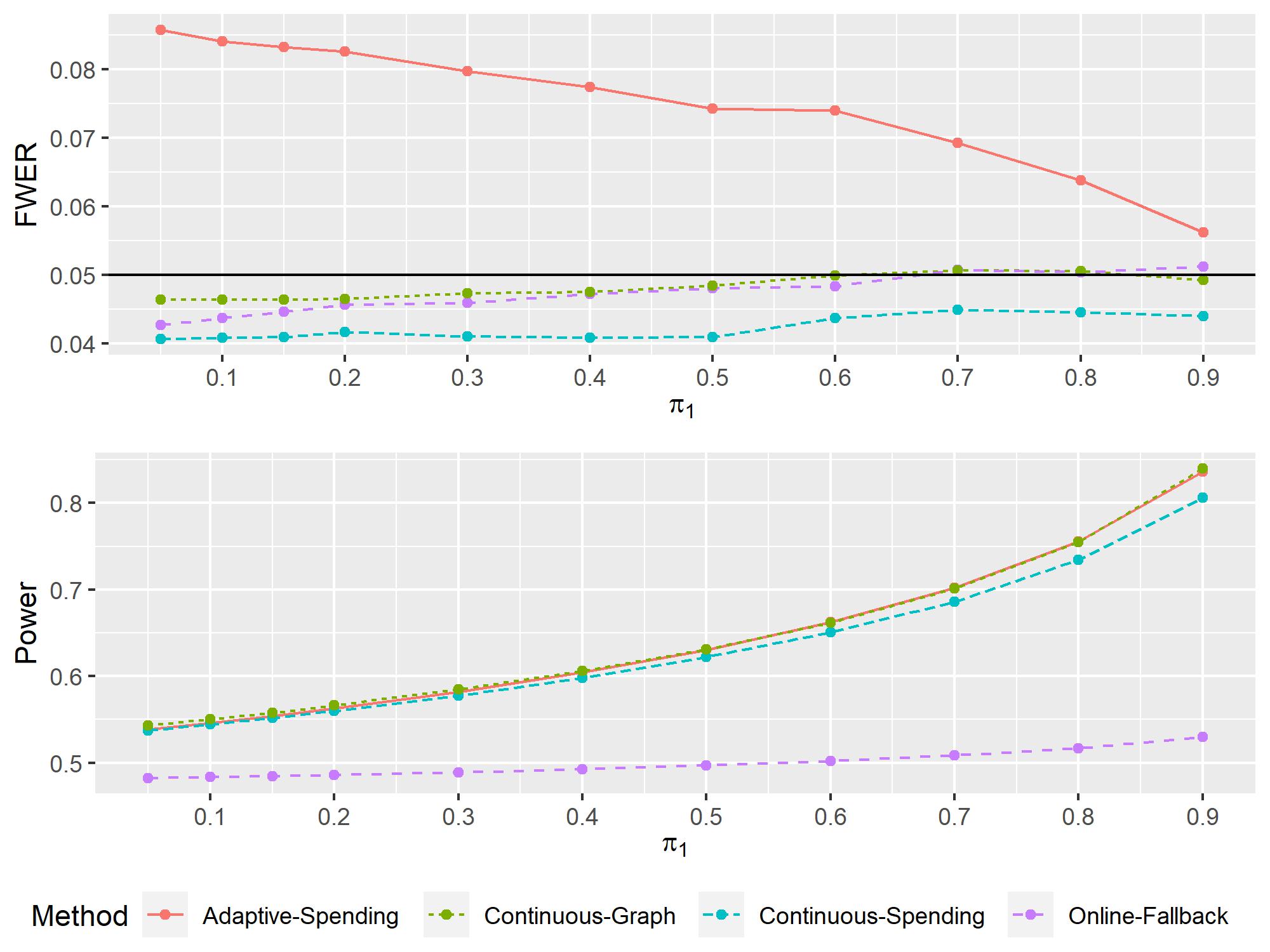
Figure 2: Estimated FWER and power in an autocorrelation set-up with $\rho=0.8$ and target level $\alpha=0.05$ plotted over the proportion of false null hypotheses $\pi_{1}$.

It can be seen in Figure 2 that the Continuous-Spending, Continuous-Graph and Online-Fallback seem to control the FWER at the nominal level $\alpha$. Only the Adaptive-Spending shows a substantial inflation of 60 %, when the proportion of false null hypotheses is small, that decreases gradually to 20 %, as the proportion of false null hypotheses increases. In terms of power, it is apparent that the Online-Fallback procedure performs considerably worse than the other three procedures, which is no surprise, as it is the only procedure without a proper built-in mechanism for adaption to the number of true null hypotheses. Here, the Continuous-Graph and the Adaptive-Spending are virtually indistinguishable, while both of them seem to be slightly more powerful than the Continuous-Spending, where the difference becomes clearer for larger values of $\pi_{1}$. Overall, the procedures for asymptotic error control seem to work well even with a finite sample size. One illustrative explanation is that the usage of the consistent weights, or more concretely the low intensity bootstrap, in a sense reduces the degree of dependence within the information used to construct the test levels, so that the resulting procedures are comparatively more robust to correlations within the $p$-values.

4.2 Platform trial

We follow the set-up described in [14]. Let $T_{1},\dots,T_{N}$ be treatments that enter the platform trial at time points $t_{1},\dots,t_{N}$, respectively. Throughout the trial patients are allocated at a uniform rate to the active treatment arms and the common control arm $C$. The responses are given as gaussian random variables $X_{ij}\sim\mathcal{N}(\mu_{i},\sigma^{2})$, $i=0,\dots,N$ with known standard deviation $\sigma$. The index 0 corresponds to the control patients. A treatment is generated as effective with probability $\pi_{1}$. We set $\mu_{i}=0$ if $T_{i}$ is ineffective, $\mu_{i}=0.5$ if it is effective and $\mu_{0}=0$. For simplicity we assume that there will be $n$ patients recruited to each treatment arm $T_{i}$, when the according test is eventually performed. Due to the uniform recruitment rate, there will be also $n$ concurrent control patients for each treatment arm. Let $\mathcal{J}_{i}$ be the index set of the concurrent control observations for the treatment arm $T_{i}$. The test statistic for the $i$-th test is of the form

$$Z_{i}=\frac{\overline{X}_{i}-\overline{X}^{(i)}_{0}}{\sigma\sqrt{\frac{2}{n}}},$$

where $\overline{X}_{i}=\frac{1}{n}\sum_{j=1}^{n}X_{ij}$ and $\overline{X}^{(i)}_{0}=\frac{1}{n}\sum_{j\in\mathcal{J}_{i}}X_{0j}$. We assume that per unit time there will be 10 patients allocated to all active treatment arms and the control arm. The time point, when the treatment $T_{i}$ enters the trial is given by $t_{i}=2(i-1)$. Similar to the previous setting, the random variables $\xi_{i,n}$ are calculated via a parametric low intensity bootstrap in treatment and control group, respectively (see Appendix for the derivation). We choose $\alpha=0.05$, $\sigma=1$ and $n=100$ (so every treatment arm stays in the trial for 10 units of time). For the number of overall treatments we consider $N\in\{30,50,100\}$ and in each case we perform 20000 independent runs for the estimation of the FWER and power.

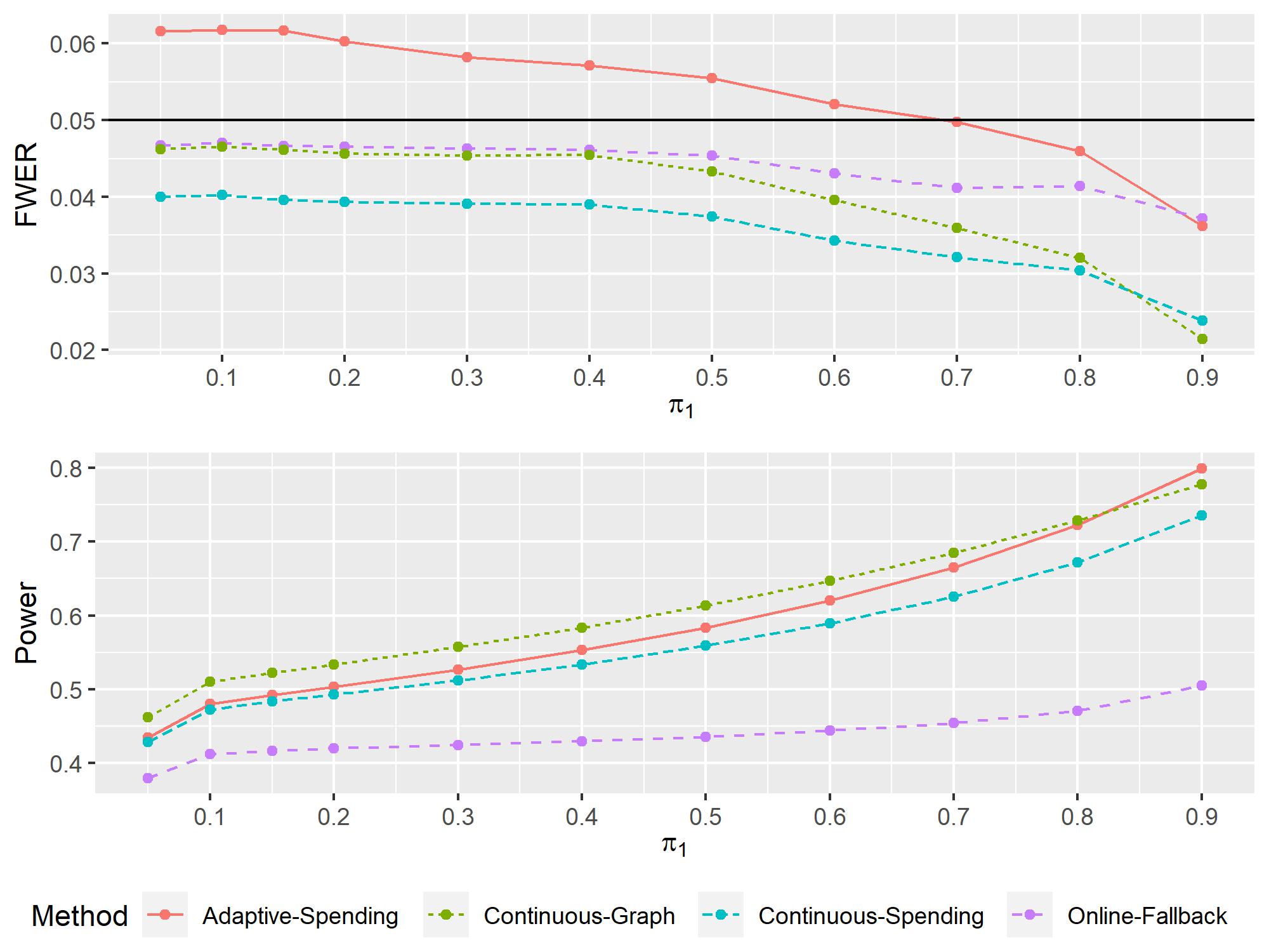
Figure 3: Estimated FWER and power in a platform trial scenario with $N=50$ and target level $\alpha=0.05$ plotted over the proportion of false null hypotheses $\pi_{1}$.

As can be seen in Figure 3, all procedures besides Adaptive-Spending control the FWER. The latter has a moderate error inflation, when $\pi_{1}$ is smaller than $0.6$. It is noticeable that the procedures (especially Continuous-Graph and Continuous-Spending) become quiet conservative when the proportion of true alternatives is high. One possible reason for this is, that the number of actually tested hypotheses in this set-up is comparatively small and a considerable proportion of the regained test level is „wasted“ on future hypotheses. This might be counteracted by a different choice of the hyperparameters $(\gamma_{i}),(g_{j,i})$ and $f$. Like in the first setting, we further see that Adaptive-Spending and the Continuous-Graph are the most powerful procedures, after that comes the Continuous-Spending and Online-Fallback is again the least powerful method by far.

5 Discussion

Existing advanced online multiple testing procedures only guarantee FWER control under the assumption of either independent or at most locally dependent $p$-values. In practice, independence is an unrealistic assumption and even methods that work for local dependence can not be applied in some situations, e.g. when the dependence of $p$-values cannot be linked to the intervening time alone or when there is little or no information about the dependency structure at all. In this work we proposed a way to derive online procedures that asymptotically control the familywise error rate, regardless of the underlying dependency structure. To this end, we established general rules for deriving new procedures and gave concrete examples. Moreover, we showed how to obtain further improvements of those procedures by using the online closure principle. In a simulation study, we showed that the asymptotic results are also satisfactory for a moderate finite sample size.

One current shortcoming is that, although the most powerful procedures developed for the case of independent (or locally dependent) $p$-values use a combination of adaptivity and discarding, only the concept of adaptivity could be transferred to this new setting, so far. This has the consequence that the proposed procedures for dependent $p$-values will lose power, when the $p$-values are conservative, i.e. being stochastically larger than a standard uniform random variable. Interesting is, that in [14] Robertson et al. did not detect any error inflation of the ADDIS-Spending procedure, which grants formal FWER control only for independent $p$-values, while we saw in Section 4 that the Adaptive-Spending exceeds the nominal test level in a similar simulation set-up. So, it seems that the additional discarding not only improves the power, but somehow also helps to maintain the nominal test level in this case. It might be interesting to investigate how this would behave if the $p$-values were negatively dependent. In any case, it would be desirable to incorporate any form of discarding or another method for dealing with conservative $p$-values into the new framework.

Another task for the future would be the extension to more general test set-ups, as only one-sided 1-sample and 2-sample hypothesis tests have been considered in this work. Similar resampling schemes can probably be used to obtain consistent weights in different situations, e.g. regression models.

In addition, there is still interest in developing more efficient methods for testing an initially unknown but finite number of hypotheses. Improvements could be expected here if the design of the procedures takes into account that ultimately only finitely many hypotheses are tested.

Appendix

Deferred proofs and derivations

Proof that the continuous Adaptive-Graph fulfills condition (6): Since no asymptotic arguments are required within this proof, we omit the index $n$ throughout. We follow the corresponding proof for the ADDIS-Graph in [6]. Let $(\alpha_{i})_{i\in\mathbb{N}}$ be the test levels of the continuous Adaptive-Graph as defined in (9). We need to show that for every $i\in\mathbb{N}$ it holds that

$$\sum_{j=1}^{i}\frac{\alpha_{j}}{1-\lambda_{j}}\xi_{j}\leq\alpha.$$

We fix an $i\in\mathbb{N}$ and define $U_{j}=1-\xi_{j}$ for $j\in\{1,\dots,i\}$. Then the claim is equivalent to

$$F_{i}(U_{1:i}):=\sum_{j=1}^{i}\left(\alpha\gamma_{j}+\sum_{k=1}^{j-1}g_{k,j}U_{k}\alpha_{k}(U_{1:k-1})\frac{1}{1-\lambda_{k}}\right)\cdot(1-U_{j})\leq\alpha$$ (15)

for any $U_{1:i}=(U_{1},\dots,U_{i})^{T}\in[0,1]^{i}$. First, consider the special case $U_{1:i}^{0}:=(0,\dots,0)^{T}\in[0,1]^{i}$, which obviously satisfies (15), since $F_{i}(U_{1:i}^{0})=\sum_{j=1}^{i}\alpha\gamma_{j}\leq\alpha$. Now, let $U_{1:i}=(U_{1},\dots,U_{i})^{T}\in[0,1]^{i}$ be arbitrary but fixed. The plan is to show that $F_{i}(U_{1:i})\leq F_{i}(U_{1:i}^{0})$, which would conclude the proof. Without loss of generality, we assume that $U_{j}>0$ for at least one $j\in\{1,\dots,i\}$ as we have already dealt with the case of all entries being zero. Furthermore, define $l=\max\{j\in\{1,\dots,i\}:U_{j}>0\}$ and consider $U_{1:i}^{l}=(U_{1}^{l},\dots,U_{i}^{l})^{T}$, where $U_{j}^{l}=U_{j}$ if $j\neq l$ and $U_{l}^{l}=0$. For ease of notation we write from now on $\alpha_{j}$ and $\alpha_{j}^{l}$ instead of $\alpha_{j}(U_{1:j-1})$ and $\alpha_{j}(U_{1:j-1}^{l})$, respectively. By the definition of $l$ and $U_{1:i}^{l}$, for every $j\leq i$ we have that $U_{j}^{l}=0$ for $j\geq l$, $U_{j}=0$ for $j\geq l+1$ and $\alpha_{j}^{l}=\alpha_{j}$ for $j\leq l$. Thus, we obtain

$$F_{i}(U_{1:i}^{l})-F_{i}(U_{1:i}) =\sum_{j=1}^{i}\alpha\gamma_{j}(U_{j}-U_{j}^{l})+\sum_{j=1}^{i}\left(\sum_{k=1}^{j-1}g_{k,j}U_{k}^{l}\alpha_{k}^{l}\frac{1}{1-\lambda_{k}}\right)\cdot(1-U_{j}^{l})$$

$$\leavevmode\nobreak\ \leavevmode\nobreak\ \leavevmode\nobreak\ \leavevmode\nobreak\ -\sum_{j=1}^{i}\left(\sum_{k=1}^{j-1}g_{k,j}U_{k}\alpha_{k}\frac{1}{1-\lambda_{k}}\right)\cdot(1-U_{j})$$

$$=\alpha\gamma_{l}U_{l}+\sum_{k=1}^{l-1}g_{k,l}U_{k}^{l}\alpha_{k}^{l}\frac{1}{1-\lambda_{k}}-(1-U_{l})\sum_{k=1}^{l-1}g_{k,l}U_{k}\alpha_{k}\frac{1}{1-\lambda_{k}}$$

$$\leavevmode\nobreak\ \leavevmode\nobreak\ \leavevmode\nobreak\ \leavevmode\nobreak\ +\sum_{j=l+1}^{i}\left(\sum_{k=1}^{j-1}g_{k,j}U_{k}^{l}\alpha_{k}^{l}\frac{1}{1-\lambda_{k}}\right)-\sum_{j=l+1}^{i}\left(\sum_{k=1}^{j-1}g_{k,j}U_{k}\alpha_{k}\frac{1}{1-\lambda_{k}}\right)$$

$$=\alpha\gamma_{l}U_{l}+U_{l}\sum_{k=1}^{l-1}g_{k,l}U_{k}\alpha_{k}\frac{1}{1-\lambda_{k}}-\sum_{j=l+1}^{i}g_{l,j}U_{l}\alpha_{l}\frac{1}{1-\lambda_{l}}$$

$$\geq U_{l}\left(\alpha\gamma_{l}+\sum_{k=1}^{l-1}g_{k,l}U_{k}\alpha_{k}\frac{1}{1-\lambda_{k}}-\alpha_{l}\frac{1}{1-\lambda_{l}}\right)\stackrel{{\scriptstyle\eqref{def_test_levels_dependent_graphgeneral_case}}}{{=}}0,$$

where the inequality holds, because $\sum_{j>l}g_{l,j}\leq 1$ and $U_{l},\alpha_{l},(1-\lambda_{l})^{-1}\geq 0$. So, we have $F_{i}(U_{1:i})\leq F_{i}(U_{1:i}^{l})$. Iterating this process, it follows that $F_{i}(U_{1:i})\leq F_{i}(U_{1:i}^{0})$, which completes the proof.

$\square$

Proof that the continuous Adaptive-Graph is a generalization of the procedure in Example 3.8: Let $\lambda_{i},\Pi\in(0,1)$, $\gamma_{i}=\Pi(1-\Pi)^{i-1},i\in\mathbb{N}$, and $g_{j,i}=\gamma_{i-j}$ for all $j\in\mathbb{N},i>j$. Further, let $\alpha_{i,n}^{\text{Graph}}$ and $\tilde{\alpha}_{i,n}$ denote the test levels of the continuous Adaptive-Graph (9) and the geometric spending algorithm (7), respectively. We give a proof by induction. By definition it holds that

$$\alpha_{1,n}^{\text{Graph}}=(1-\lambda_{1})\gamma_{1}\alpha=(1-\lambda_{1})\Pi\alpha=\tilde{\alpha}_{1,n}.$$

Now assume that $\alpha_{i,n}^{\text{Graph}}=\tilde{\alpha}_{i,n}$ holds for an $i\in\mathbb{N}$. Then,

$$\alpha_{i+1,n}^{\text{Graph}} =(1-\lambda_{i+1})\left(\gamma_{i+1}\alpha+\sum_{j=1}^{i}\gamma_{i-j+1}(1-\xi_{j,n})\frac{\alpha_{j,n}^{\text{Graph}}}{1-\lambda_{j}}\right)$$

$$=(1-\lambda_{i+1})\left((1-\Pi)\gamma_{i}\alpha+\Pi(1-\xi_{i,n})\frac{\alpha_{i,n}^{\text{Graph}}}{1-\lambda_{i}}+(1-\Pi)\sum_{j=1}^{i-1}\gamma_{i-j}(1-\xi_{j,n})\frac{\alpha_{j,n}^{\text{Graph}}}{1-\lambda_{j}}\right)$$

$$=(1-\lambda_{i+1})\left(\Pi(1-\xi_{i,n})\frac{\alpha_{i,n}^{\text{Graph}}}{1-\lambda_{i}}+(1-\Pi)\frac{\alpha_{i,n}^{\text{Graph}}}{1-\lambda_{i}}\right)$$

$$=(1-\lambda_{i+1})\frac{\alpha_{i,n}^{\text{Graph}}}{1-\lambda_{i}}(1-\Pi\xi_{i,n})$$

$$=(1-\lambda_{i+1})\frac{\tilde{\alpha}_{i,n}}{1-\lambda_{i}}(1-\Pi\xi_{i,n})$$

$$\stackrel{{\scriptstyle\eqref{def_testlevel_uniform_recursion}}}{{=}}\tilde{\alpha}_{i+1,n}.$$

The recursion formula (8) holds, because for the general test levels (7) we have that

$$\alpha_{i+1,n} =\Pi_{i+1}(1-\lambda_{i+1})\cdot\left(\alpha-\sum_{j<i+1}\frac{\alpha_{j,n}}{1-\lambda_{j}}\xi_{j,n}\right)$$

$$=\Pi_{i+1}(1-\lambda_{i+1})\cdot\left(\frac{\alpha_{i,n}}{(1-\lambda_{i})\Pi_{i}}-\frac{\alpha_{i,n}}{1-\lambda_{i}}\xi_{i,n}\right)$$

$$=\Pi_{i+1}(1-\lambda_{i+1})\cdot\frac{\alpha_{i,n}(1-\Pi_{i}\xi_{i,n})}{(1-\lambda_{i})\Pi_{i}}.$$

$\square$

Computation of the constant for the interpolation procedure (12): We compute

$$\int_{1}^{\infty}f_{\gamma}(x)dx =\sum_{k=1}^{\infty}\int_{k}^{k+1}f_{\gamma}(x)dx$$

$$=\sum_{k=1}^{\infty}\int_{k}^{k+1}\left(\gamma_{k}+(x-k)\cdot(\gamma_{k+1}-\gamma_{k})\right)dx$$

$$=\sum_{k=1}^{\infty}\left(\gamma_{k}+\int_{0}^{1}x\cdot(\gamma_{k+1}-\gamma_{k})dx\right)$$

$$=\frac{1}{2}\left(\sum_{k=1}^{\infty}\gamma_{k}+\sum_{k=2}^{\infty}\gamma_{k}\right)$$

$$=1-\frac{\gamma_{1}}{2}.$$

Since $f_{\gamma}(1)=\gamma_{1}$, we have $s=(1-\lambda)f_{\gamma}(1)+\int_{1}^{\infty}f_{\gamma}(x)dx=1+\gamma_{1}(0.5-\lambda)$.

Proof of Lemma 3.10: Let $j_{1}<j_{2}<\dots<j_{k}$ denote the indices corresponding to the true null hypotheses among the first $N$ hypotheses and let $0<\varepsilon<1-\lambda$. Due to (5) there exists an $n_{0}\in\mathbb{N}$ such that for all $n\geq n_{0}$ we have $\mathbb{P}(1-\lambda-\xi_{i,n}\geq\varepsilon)\leq\frac{\varepsilon}{k}$ (for all $i\in\mathcal{H}^{0}=\mathcal{H}^{0}(N)$). For the test levels defined in (10) it holds that

$$\mathbb{E}\left(\sum_{i\in\{1,\dots,k\}}\alpha_{j_{i},n}\right) \leq\mathbb{E}\left(\frac{\alpha}{s}\cdot\sum_{i\in\{1,\dots,k\}}(1-\lambda)f(1+\sum_{l<i}\xi_{j_{l},n})\right)$$

$$=\frac{\alpha}{s}\cdot\mathbb{E}\left((1-\lambda)f(1)+\sum_{i\in\{2,\dots,k\}}\mathds{1}\{\xi_{j_{i-1},n}>1-\lambda-\varepsilon\}(1-\lambda)f(1+\sum_{l<i}\xi_{j_{l},n})\right)$$

$$\phantom{{}=1}+\frac{\alpha}{s}\cdot\mathbb{E}\left(\sum_{i\in\{2,\dots,k\}}\mathds{1}\{\xi_{j_{i-1},n}\leq 1-\lambda-\varepsilon\}(1-\lambda)f(1+\sum_{l<i}\xi_{j_{l},n})\right)$$

$$\leq\frac{\alpha}{s}\cdot\mathbb{E}\left((1-\lambda)f(1)+\sum_{i\in\{2,\dots,k\}}\mathds{1}\{\xi_{j_{i-1},n}>1-\lambda-\varepsilon\}\frac{1-\lambda}{\xi_{j_{i-1},n}}\int_{1+\sum_{l<i-1}\xi_{j_{l},n}}^{1+\sum_{l<i}\xi_{j_{l},n}}f(x)dx\right)$$

$$\phantom{{}=1}+\frac{\alpha}{s}\cdot(1-\lambda)\cdot f(1)\sum_{i\in\{2,\dots,k\}}\mathbb{P}(\xi_{j_{i-1},n}\leq 1-\lambda-\varepsilon)$$

$$\leq\frac{\alpha}{s}\cdot\mathbb{E}\left((1-\lambda)f(1)+\sum_{i\in\{2,\dots,k\}}\frac{1-\lambda}{1-\lambda-\varepsilon}\int_{1+\sum_{l<i-1}\xi_{j_{l},n}}^{1+\sum_{l<i}\xi_{j_{l},n}}f(x)dx\right)$$

$$\phantom{{}=1}+\alpha\cdot\sum_{i\in\{2,\dots,k\}}\frac{\varepsilon}{k}$$

$$\leq\frac{\alpha}{s}\cdot\mathbb{E}\left(\frac{1-\lambda}{1-\lambda-\varepsilon}\cdot(1-\lambda)f(1)+\sum_{i\in\{2,\dots,k\}}\frac{1-\lambda}{1-\lambda-\varepsilon}\int_{1+\sum_{l<i-1}\xi_{j_{l},n}}^{1+\sum_{l<i}\xi_{j_{l},n}}f(x)dx\right)+\varepsilon$$

$$\leq\frac{\alpha}{s}\cdot\frac{1-\lambda}{1-\lambda-\varepsilon}\cdot\mathbb{E}\left((1-\lambda)f(1)+\int_{1}^{\infty}f(x)dx\right)+\varepsilon$$

$$=\alpha\cdot\frac{(1-\lambda)}{1-\lambda-\varepsilon}+\varepsilon.$$

Here, in the first and second inequality it is used, that $f$ is non-increasing. As $\varepsilon$ was arbitrary, we conclude $\lim_{n\rightarrow\infty}\mathbb{E}\left(\sum_{i\in\{1,\dots,k\}}\alpha_{j_{i},n}\right)\leq\alpha$. Since $\alpha_{i,n}\stackrel{{\scriptstyle\text{a.s.}}}{{\rightarrow}}\alpha_{i}$, we also have $\sum_{i\in\mathcal{H}^{0}}\alpha_{i,n}\stackrel{{\scriptstyle\text{a.s.}}}{{\rightarrow}}\sum_{i\in\mathcal{H}^{0}}\alpha_{i}$. The dominated convergence theorem plus the fact that $\sum_{i\in\mathcal{H}^{0}}\alpha_{i,n}\leq k$ then yield

$$\alpha\geq\mathbb{E}(\sum_{i\in\mathcal{H}^{0}}\alpha_{i})=\sum_{i\in\mathcal{H}^{0}}\alpha_{i}.$$

$\square$

Derivation of the closed procedures (13) and (14): Based on the test levels (9), for every $I\subseteq\mathbb{N}$ we consider the intersection test that rejects the intersection hypothesis $H_{I}=\bigcap_{i\in I}H_{i}$ if and only if for at least one $i\in I$ it holds that

$$P_{i,n}\leq\alpha_{i,n}^{I}:=(1-\lambda_{i})\left(\alpha\gamma_{i}+\sum_{j\in I,j<i}g_{j,i}(1-\xi_{j,n})\frac{\alpha_{j,n}^{I}}{1-\lambda_{j}}+\sum_{j\notin I,j<i}g_{j,i}\frac{\alpha_{j,n}^{(I\cup\{j\})}}{1-\lambda_{j}}\right).$$

Note that $\alpha_{1,n}^{I}=(1-\lambda_{1})\cdot\alpha\gamma_{i}$ if $1\in I$ and all further test levels are defined recursively. It is easy to see, that this defines a predictable and consonant intersection test (with the terminology as in [5]), since the test levels depend only on previous indices and for any $i\in I$ it holds that $\alpha_{i,n}^{I}\leq\alpha_{i,n}^{J}$ for all $J\subseteq I$ with $i\in J$. Moreover, it is an (asymptotical) level $\alpha$ test, as it fulfills (6) (with the summation only taking place over the index set $I$), because the original procedure (9) does and the case $j\notin I$ can be interpreted as $\xi_{j,n}=0$. Now, we recursively define $I_{1}=\{1\}$ and $I_{i}=\{j\in\mathbb{N}:j<i,P_{j,n}>\alpha_{j,n}^{I_{j}}\}\cup\{i\}$ for $i\geq 2$. The short-cut procedure according to [5] is then given by

$$\alpha_{i,n}=\alpha_{i,n}^{I_{i}}=(1-\lambda_{i})\left(\alpha\gamma_{i}+\sum_{j<i}g_{j,i}\max\{1-\xi_{j,n},R_{j,n}\}\frac{\alpha_{j,n}}{1-\lambda_{j}}\right).$$

Analogous, the test levels for the intersection tests based on the procedure (10) are defined as

$$\alpha_{i,n}^{I}:=\alpha\cdot\frac{(1-\lambda)}{s}\cdot f\left(1+\sum_{j\in I,j<i}\xi_{j,n}\right).$$

Again, it is easy to verify that these intersection tests are predictable and consonant. Furthermore, they are asymptotical level $\alpha$ tests, as can be seen by slightly modifying the proof of Lemma 3.10. With $I_{i}$ as above, the short-cut procedure is given by

$$\alpha_{i,n}=\alpha_{i,n}^{I_{i}}=\alpha\cdot\frac{(1-\lambda)}{s}\cdot f\left(1+\sum_{j<i}\xi_{j,n}\cdot(1-R_{j,n})\right).$$

Obtaining consistent weights in a 2-sample design: Assume that the observed data $\mathcal{X}$ consists of independent random variables $X_{1},\dots,X_{n_{1}}\sim\mathcal{N}(\mu^{X},1),Y_{1},\dots,Y_{n_{2}}\sim\mathcal{N}(\mu^{Y},1)$ and we want to test the hypothesis $H:\mu^{X}-\mu^{Y}\leq 0$ versus the alternative $H^{\prime}:\mu^{X}-\mu^{Y}>0$. Here, $n_{1}=n_{1}(n)$ and $n_{2}=n_{2}(n)$ are the sample sizes for the respective groups, which depend implicitly on the overall asymptotic parameter $n$. The test statistic and the corresponding one-sided $p$-value are given by $Z_{n}=(1/n_{1}+1/n_{2})^{-0.5}(\overline{X}_{n_{1}}-\overline{Y}_{n_{2}})$ and $P_{n}=1-\Phi(Z_{n})$, respectively. Similar to Example 3.2 consider the parametric bootstrap variables $X_{1}^{*},\dots,X_{m(n_{1})}^{*},Y_{1}^{*},\dots,Y_{m(n_{2})}^{*}$, which are independently drawn from the distributions $\mathcal{N}(\overline{X}_{n_{1}},1)$ and $\mathcal{N}(\overline{Y}_{n_{2}},1)$, respectively. As before, $m:\mathbb{N}\longrightarrow\mathbb{N}$ is a non-decreasing map s.t. $m(n)\to\infty$ and $\frac{m(n)}{n}\to 0$ as $n\to\infty$. Furthermore, we construct the (low intensity) bootstrap test statistic

$$Z_{m(n)}^{*}=\frac{1}{\sqrt{1/m(n_{1})+1/m(n_{2})}}\left(m(n_{1})^{-1}\sum_{j=1}^{m(n_{1})}X_{j}^{*}-m(n_{2})^{-1}\sum_{j=1}^{m(n_{2})}Y_{j}^{*}\right),$$

whose conditional distribution is given by a normal distribution with variance 1 and mean

$$\sqrt{\frac{1/n_{1}+1/n_{2}}{1/m(n_{1})+1/m(n_{2})}}Z_{n}.$$

Moreover, we define the low intensity bootstrap version of the $p$-value $P_{n}$ by $P_{m(n)}^{*}=1-\Phi(Z^{*}_{m(n)})$. For any $\lambda\in(0,1)$, we can now define the consistent weights by $\xi_{n}=\mathbb{P}(P_{m(n)}^{*}>\lambda|\mathcal{X})$. The consistency condition (5) can be shown completely analogous to Example 3.2 if $n_{1}=n_{2}$. In general, it is necessary that the groups are at least asymptotically balanced, i.e. $\frac{n_{1}}{n_{2}}\to 1$ as $n\to\infty$.

Further simulation results

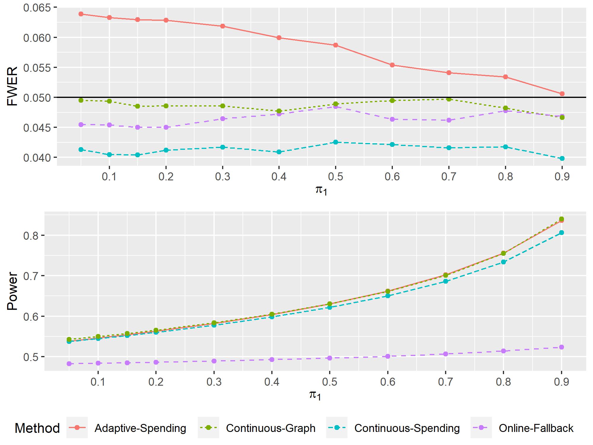
Figure 4: Estimated FWER and power in an autocorrelation set-up with $\rho=0.5$ and target level $\alpha=0.05$ plotted over the proportion of false null hypotheses $\pi_{1}$.

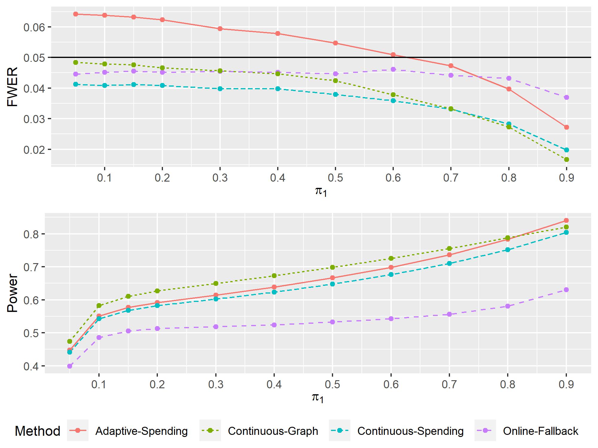
Figure 5: Estimated FWER and power in a platform trial scenario with $N=30$ and target level $\alpha=0.05$ plotted over the proportion of false null hypotheses $\pi_{1}$.

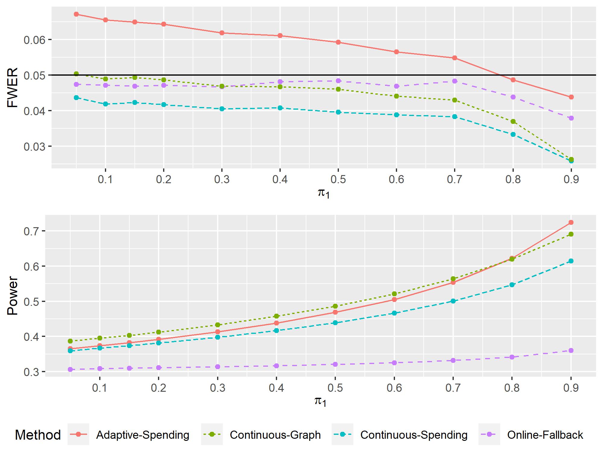
Figure 6: Estimated FWER and power in a platform trial scenario with $N=100$ and target level $\alpha=0.05$ plotted over the proportion of false null hypotheses $\pi_{1}$.

Supplementary Material

The R source code used for the simulations is available under https://github.com/vijankovic/Online-Procedures-Dependency.

References

- [1] Ehud Aharoni and Saharon Rosset. Generalized -investing: definitions, optimality results and application to public databases. Journal of the Royal Statistical Society: Series B: Statistical Methodology, pages 771–794, 2014.
- [2] Peter J Bickel, Friedrich Götze, and Willem R van Zwet. Resampling fewer than n observations: gains, losses, and remedies for losses. Springer, 2012.
- [3] Peter J Bickel and Anat Sakov. On the choice of m in the m out of n bootstrap and confidence bounds for extrema. Statistica Sinica, pages 967–985, 2008.
- [4] Jean Feng, Gene Pennllo, Nicholas Petrick, Berkman Sahiner, Romain Pirracchio, and Alexej Gossmann. Sequential algorithmic modification with test data reuse. In Uncertainty in Artificial Intelligence, pages 674–684. PMLR, 2022.
- [5] Lasse Fischer, Marta Bofill Roig, and Werner Brannath. The online closure principle. arXiv preprint arXiv:2211.11400, 2022.
- [6] Lasse Fischer, Marta Bofill Roig, and Werner Brannath. An adaptive-discard-graph for online error control. arXiv preprint arXiv:2301.11711, 2023.
- [7] Aaron Fisher. Saffron and lord ensure online control of the false discovery rate under positive dependence. arXiv preprint arXiv:2110.08161, 2021.
- [8] Dean P Foster and Robert A Stine. -investing: a procedure for sequential control of expected false discoveries. Journal of the Royal Statistical Society: Series B (Statistical Methodology), 70(2):429–444, 2008.
- [9] Adel Javanmard and Andrea Montanari. Online rules for control of false discovery rate and false discovery exceedance. The Annals of statistics, 46(2):526–554, 2018.
- [10] Ruth Marcus, Peritz Eric, and K Ruben Gabriel. On closed testing procedures with special reference to ordered analysis of variance. Biometrika, 63(3):655–660, 1976.
- [11] André Neumann, Taras Bodnar, and Thorsten Dickhaus. Estimating the proportion of true null hypotheses under dependency: A marginal bootstrap approach. Journal of Statistical Planning and Inference, 210:76–86, 2021.
- [12] Aaditya Ramdas, Tijana Zrnic, Martin Wainwright, and Michael Jordan. Saffron: an adaptive algorithm for online control of the false discovery rate. In International conference on machine learning, pages 4286–4294. PMLR, 2018.
- [13] David S Robertson, James Wason, and Aaditya Ramdas. Online multiple hypothesis testing for reproducible research. arXiv preprint arXiv:2208.11418, 2022.
- [14] David S Robertson, James MS Wason, Franz König, Martin Posch, and Thomas Jaki. Online error rate control for platform trials. Statistics in Medicine, 2023.
- [15] Anat Sakov. Using the m out of n bootstrap in hypothesis testing. University of California, Berkeley, 1998.
- [16] Jan WH Swanepoel. A note on proving that the (modified) bootstrap works. Communications in Statistics-Theory and Methods, 15(11):3193–3203, 1986.
- [17] Jinjin Tian and Aaditya Ramdas. Online control of the familywise error rate. Statistical Methods in Medical Research, 30(4):976–993, 2021.
- [18] Sonja Zehetmayer, Martin Posch, and Franz Koenig. Online control of the false discovery rate in group-sequential platform trials. Statistical Methods in Medical Research, 31(12):2470–2485, 2022.
- [19] Tijana Zrnic, Aaditya Ramdas, and Michael I Jordan. Asynchronous online testing of multiple hypotheses. The Journal of Machine Learning Research, 22(1):1585–1623, 2021.