Port-Hamiltonian Neural ODE Networks on Lie Groups For Robot Dynamics Learning and Control

Abstract

Accurate models of robot dynamics are critical for safe and stable control and generalization to novel operational conditions. Hand-designed models, however, may be insufficiently accurate, even after careful parameter tuning. This motivates the use of machine learning techniques to approximate the robot dynamics over a training set of state-control trajectories. The dynamics of many robots are described in terms of their generalized coordinates on a matrix Lie group, e.g. on $SE(3)$ for ground, aerial, and underwater vehicles, and generalized velocity, and satisfy conservation of energy principles. This paper proposes a (port-)Hamiltonian formulation over a Lie group of the structure of a neural ordinary differential equation (ODE) network to approximate the robot dynamics. In contrast to a black-box ODE network, our formulation guarantees energy conservation principle and Lie group’s constraints by construction and explicitly accounts for energy-dissipation effect such as friction and drag forces in the dynamics model. We develop energy shaping and damping injection control for the learned, potentially under-actuated Hamiltonian dynamics to enable a unified approach for stabilization and trajectory tracking with various robot platforms.

Supplementary Material

Software and videos supplementing this paper:

https://thaipduong.github.io/LieGroupHamDL

I Introduction

Motion planning and optimal control algorithms depend on the availability of accurate system dynamics models. Models obtained from first principles and calibrated over a small set of parameters via system identification [1] are widely used for unmanned ground vehicles (UGVs), unmanned aerial vehicles (UAVs), and unmanned underwater vehicles (UUVs). Such models may over-simplify or even incorrectly describe the underlying structure of the dynamical system, leading to bias and modeling errors that cannot be corrected by adjusting a few parameters. Data-driven techniques [2, 3, 4, 5, 6] have emerged as a powerful approach to approximate system dynamics with an over-parameterized machine learning model, trained over a dataset of system state and control trajectories. Neural networks are expressive function approximation models, capable of identifying and generalizing interaction patterns from the training data. Training neural network models, however, typically requires large amounts of data and computation time, which may be impractical in mobile robotics applications. Recent works [7, 8, 9, 10, 11, 12, 13, 14] have considered a hybrid approach, where prior knowledge of the physics, governing the system dynamics, is used to assist the learning process. The dynamics of physical systems obey kinematic constraints and energy conservation laws. These laws are known to be universally true but a black-box machine learning model might struggle to infer them from the training data, causing poor generalization. Instead, prior knowledge may be encoded into the learning model, e.g., using a prior distribution [3], a graph-network forward kinematic model [15], or a network architecture reflecting the structure of Lagrangian [16] or Hamiltonian [10] mechanical systems. Moreover, many physical robot platforms are composed of rigid-body interconnections and their state evolution respects the structure of a Lie group [17], e.g., the position and orientation kinematics of a rigid body evolve on the $SE(3)$ Lie group [18].

The goal of this paper is to incorporate both the kinematic structure and the energy conservation properties of physical systems with Lie group states into the structure of a dynamics learning model. We also aim to design a control approach that achieves stabilization or trajectory tracking using the learned model without requiring prior knowledge of its parameters. In other words, the same control design should enable trajectory tracking for learned models of different rigid-body UGVs, UAVs, or UUVs.

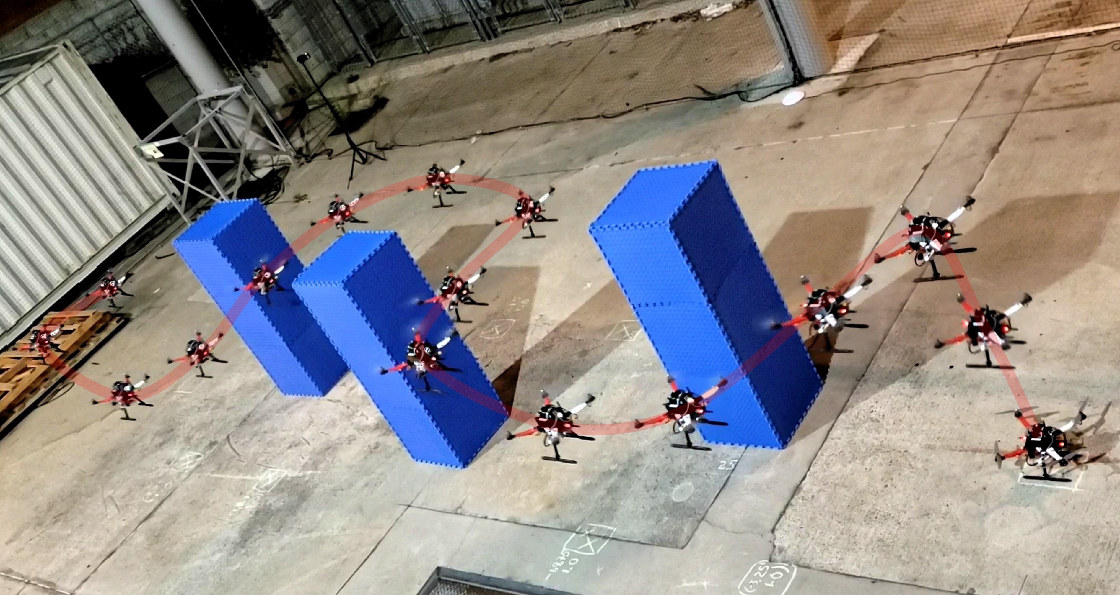
Figure 1: Quadrotor trajectory tracking using a learned port-Hamiltonian dynamics model.

Lagrangian and Hamiltonian mechanics [19, 20] provide physical system descriptions that can be integrated into the structure of a neural network [10, 21, 11, 22, 23, 24]. Prior work, however, has only considered vector-valued states, when designing Lagrangian- or Hamiltonian-structured neural networks. This limits the applicability of these techniques as many common robot systems have states on a Lie group. For example, Hamiltonian equations of motion are available for orientation but existing formulations rely predominantly on $3$ dimensional vector parametrizations, such as Euler angles [25, 26], which suffer from singularities. In our preliminary work [27], we design a neural ordinary differential equation (ODE) network [28], whose structure captures Hamiltonian dynamics over the $SE(3)$ manifold [29]. Our model guarantees by construction that long-term trajectory predictions satisfy $SE(3)$ constraints and conserve total energy. Inspired by [23, 30], we model kinetic energy and potential energy by separate neural networks, each governed by a set of Hamiltonian equations on $SE(3)$. The Hamiltonian formulation can be generalized to a Port-Hamiltonian one [31], enabling us to design an energy-based controller for trajectory tracking. Our preliminary work [27] is developed specifically for the $SE(3)$ manifold and does not consider dissipation elements that drain energy from the system, such as friction or drag forces. In this paper, we generalize our port-Hamiltonian neural ODE network to embed general matrix Lie group constraints and introduce an energy dissipation term, represented by another neural network, to model friction and air drag in physical systems. We verify our approach extensively with simulated robot systems, including a pendulum and a Crazyflie quadrotor, and with several real quadrotor platforms. In summary, this paper makes the following contributions.

• We design a neural ODE model that respects port-Hamiltonian dynamics over a matrix Lie group to enable data-driven learning of rigid-body system dynamics.

• We develop a unified control policy for port-Hamiltonian dynamics on a Lie group that achieves trajectory tracking if permissible by the system’s degree of underactuation.

• We demonstrate our dynamics learning and control approach with simulated robot systems (a pendulum and a quadrotor) and several real quadrotor robots.

II Related Work

Data-driven techniques [32, 33, 34, 35, 36] have shown impressive results in learning robot dynamics models from state-control trajectories. Neural networks offer especially expressive system models but their training requires large amounts of data, which may be impractical in mobile robot applications. Recently, a hybrid approach [7, 8, 9, 10, 11, 12, 13, 14, 24, 37, 38, 39] has been considered where prior knowledge about a physical system is integrated into the design of a machine learning model. Models designed with structure respecting kinematic constraints [15], symmetry [40, 41], Lagrangian mechanics [12, 16, 8, 9, 42, 7, 13] or Hamiltonian mechanics [10, 21, 11, 22, 23, 24, 14, 43, 44] guarantee that the laws of physics are satisfied by construction, regardless of the training data.

Sanchez-Gonzalez et al. [15] design graph neural networks to represent the kinematic structure of complex dynamical systems and demonstrate forward model learning and online planning via gradient-based trajectory optimization. Ruthotto et al. [40] propose a partial differential equation (PDE) interpretation of convolutional neural networks and derive new parabolic and hyperbolic ResNet architectures guided by PDE theory. Wang et al. [41] design symmetry equivariant neural network models, encoding rotation, scaling, and uniform motion, to learn physical dynamics that are robust to symmetry group distributional shifts.

Lagrangian-based methods [12, 16, 8, 9, 42, 7, 13] design neural network models for physical systems based on the Euler-Lagrange differential equations of motion [19, 20], in terms of generalized coordinates $\mathbf{{\boldsymbol{\mathfrak{q}}}}$, their velocity $\dot{\mathbf{{\boldsymbol{\mathfrak{q}}}}}$ and a Lagrangian function $\mathcal{L}(\mathbf{{\boldsymbol{\mathfrak{q}}}},\dot{\mathbf{{\boldsymbol{\mathfrak{q}}}}})$, defined as the difference between the kinetic and potential energies. The energy terms are modeled by neural networks, either separately [16, 42, 7] or together [9].

Hamiltonian-based methods [10, 21, 11, 22, 23, 24, 14] use a Hamiltonian formulation [19, 20] of the system dynamics, instead, in terms of generalized coordinates $\mathbf{{\boldsymbol{\mathfrak{q}}}}$, generalized momenta $\mathbf{{\boldsymbol{\mathfrak{p}}}}$, and a Hamiltonian function, $\mathcal{H}(\mathbf{{\boldsymbol{\mathfrak{q}}}},\mathbf{{\boldsymbol{\mathfrak{p}}}})$, representing the total energy of the system. Greydanus et al. [10] model the Hamiltonian as a neural network and update its parameters by minimizing the discrepancy between its symplectic gradients and the time derivatives of the states $(\mathbf{{\boldsymbol{\mathfrak{q}}}},\mathbf{{\boldsymbol{\mathfrak{p}}}})$. This approach, however, requires that the state time derivatives are available in the training data set. Chen et al. [11], Zhong et al. [23] relax this assumption by using differentiable leapfrog integrators [45] and differentiable ODE solvers [28], respectively. The need for time derivatives of the states is eliminated by back-propagating a loss function measuring state discrepancy through the ODE solvers via the adjoint method. Our work extends the approach in [23, 30] by formulating the Hamiltonian dynamics over a matrix Lie group, which enforces kinematic constraints in the neural ODE network used to learn the dynamics. Toth et al. [46] and Mason et al. [47] show that, instead of from state trajectories, the Hamiltonian function can be learned from high-dimensional image observations. Finzi et al. [22] show that using Cartesian coordinates with explicit constraints improves both the accuracy and data efficiency for the Lagrangian- and Hamiltonian-based approaches. In a closely related work, Zhong et al. [30] showed that dissipating elements, such as friction or air drag, can be incorporated in a Hamiltonian-based neural ODE network by reformulating the system dynamics in port-Hamiltonian form [31]. The continuous-time equations of motions in Lagrangian or Hamiltonian dynamics can also be discretized using variational integrators [48] to learn discrete-time Lagrangian and Hamiltonian systems [49, 50, 51, 52] and provide long-term prediction for control methods such as model predictive control [53]. This approach eliminates the need to use an ODE solver to roll out the dynamics but its prediction accuracy depends on the discretization time step.

While most existing dynamics learning approaches focus on Euclidean dynamics, many robot systems have states evolving on a matrix Lie group. We develop a neural ODE framework that incorporates both the law of energy conservation, via a Hamiltonian formulation, and the matrix Lie group constraints in the model. Furthermore, few dynamics learning papers consider control design based on the learned model. We develop a general trajectory tracking controller for Lie group Hamiltonian dynamics.

The Hamiltonian formulation and its port-Hamiltonian generalization [31] are built around the notion of system energy and, hence, are naturally related to control techniques for stabilization aiming to minimize the total energy. Since the minimum point of the Hamiltonian might not correspond to a desired regulation point, the control design needs to inject additional energy to ensure that the minimum of the total energy is at the desired equilibrium. For fully-actuated (port-)Hamiltonian systems, it is sufficient to shape the potential energy only using an energy-shaping and damping-injection (ES-DI) controller [31]. For underactuated systems, both the kinetic and potential energies needs to be shaped, e.g., via interconnection and damping assignment passivity-based control (IDA-PBC) [31, 54, 55, 56]. Wang and Goldsmith [57] extend the IDA-PBC controller from stabilization to trajectory tracking. Closely related to our controller design, Souza et. al. [58] apply this technique to design a controller for an underactuated quadrotor robot but use Euler angles as the orientation representation. Port-Hamiltonian structure and energy-based control design are also used to learn distributed control policies from state-control trajectories [59, 60, 61].

We connect Hamiltonian-dynamics learning with the idea of IDA-PBC control to allow stabilization of any rigid-body robot without relying on its model parameters a priori. We design a trajectory-tracking controller for underactuated systems, e.g., quadrotor robots, based on the IDA-PBC approach and show how to construct desired pose and momentum trajectories given only desired position and yaw. We demonstrate the tight integration of dynamics learning and control to achieve closed-loop trajectory tracking with underactuated quadrotor robots.

III Problem Statement

Consider a robot with state $\mathbf{x}$ consisting of generalized coordinates ${\boldsymbol{\mathfrak{q}}}$ evolving on a Lie group $\mathsf{G}$ and generalized velocity $\boldsymbol{\xi}$ on the Lie algebra ${\boldsymbol{\mathfrak{g}}}$ of $\mathsf{G}$. Let $\dot{\mathbf{x}}=\mathbf{f}(\mathbf{x},\mathbf{u})$ characterize the robot dynamics with control input $\mathbf{u}\in\mathbb{R}^{m}$. For example, the state of rigid-body mobile robot, such as a UGV or UAV, may be modeled by its pose on the $SE(3)$ group, consisting of position and orientation, and its twist on the $\mathfrak{se}(3)$ Lie algebra, consisting of linear and angular velocity. The control input of an Ackermann-drive UGV may include its linear acceleration and steering angle rate, and that of a quadrotor UAV may include the total thrust and moment generated by the propellers. See Sec. IV-C for more details.

We assume that the function $\mathbf{f}$ specifying the robot dynamics is unknown and aim to approximate it using a dataset $\mathcal{D}$ of state and control trajectories. Specifically, let ${\cal D}=\{t_{0:N}^{(i)},\mathbf{x}^{(i)}_{0:N},\mathbf{u}^{(i)}\}_{i=1}^{D}$ consist of $D$ state sequences $\mathbf{x}^{(i)}_{0:N}$, obtained by applying a constant control input $\mathbf{u}^{(i)}$ to the system with initial condition $\mathbf{x}^{(i)}_{0}$ at time $t_{0}^{(i)}$ and sampling its state $\mathbf{x}^{(i)}(t_{n}^{(i)})=:\mathbf{x}^{(i)}_{n}$ at times $t_{0}^{(i)}<t_{1}^{(i)}<\ldots<t_{N}^{(i)}$. Using the dataset $\mathcal{D}$, we aim to find a function $\bar{\mathbf{f}}_{\boldsymbol{\theta}}$ with parameters $\boldsymbol{\theta}$ that approximates the true dynamics $\mathbf{f}$ well. To optimize $\boldsymbol{\theta}$, we roll out the approximate dynamics $\bar{\mathbf{f}}_{\boldsymbol{\theta}}$ with initial state $\mathbf{x}_{0}^{(i)}$ and constant control $\mathbf{u}^{(i)}$ and minimize the discrepancy between the computed state sequence $\bar{\mathbf{x}}^{(i)}_{1:N}$ and the true state sequence $\mathbf{x}^{(i)}_{1:N}$ in ${\cal D}$.

Problem 1.

Given a dataset ${\cal D}=\{t_{0:N}^{(i)},\mathbf{x}^{(i)}_{0:N},\mathbf{u}^{(i)}\}_{i=1}^{D}$ and a function $\bar{\mathbf{f}}_{\boldsymbol{\theta}}$, find the parameters $\boldsymbol{\theta}$ that minimize:

$$\min_{\boldsymbol{\theta}} \sum_{i=1}^{D}\sum_{n=1}^{N}\ell(\mathbf{x}^{(i)}_{n},\bar{\mathbf{x}}^{(i)}_{n})$$ (1)

s.t. $$\dot{\bar{\mathbf{x}}}^{(i)}(t)=\bar{\mathbf{f}}_{\boldsymbol{\theta}}(\bar{\mathbf{x}}^{(i)}(t),\mathbf{u}^{(i)}),\;\;\bar{\mathbf{x}}^{(i)}(t_{0})=\mathbf{x}^{(i)}_{0},$$

$$\bar{\mathbf{x}}^{(i)}_{n}=\bar{\mathbf{x}}^{(i)}(t_{n}),\;\;\forall n=1,\ldots,N,\;\;\forall i=1,\ldots,D,$$

where $\ell$ is a distance metric on the state space.

Further, we aim to design a feedback controller capable of tracking a desired state trajectory $\mathbf{x}^{*}(t)$, $t\geq t_{0}$, for the learned model $\bar{\mathbf{f}}_{\boldsymbol{\theta}}$ of the robot dynamics.

Problem 2.

Given an initial condition $\mathbf{x}_{0}$ at time $t_{0}$, desired state trajectory $\mathbf{x}^{*}(t)$, $t\geq t_{0}$, and learned dynamics $\bar{\mathbf{f}}_{\boldsymbol{\theta}}$, design a feedback control law $\mathbf{u}=\boldsymbol{\pi}(\mathbf{x},\boldsymbol{\theta},\mathbf{x}^{*}(t))$ such that $\limsup_{t\to\infty}\ell(\mathbf{x}(t),\mathbf{x}^{*}(t))$ is bounded.

We consider robot kinematics on the Lie group $\mathsf{G}$ such that when there is no control input, $\mathbf{u}=\bf 0$, the dynamics $\mathbf{f}(\mathbf{x},\mathbf{u})$ respect the law of energy conservation. We embed these constraints in the structure of the parametric function $\bar{\mathbf{f}}_{\boldsymbol{\theta}}$. We review matrix Lie groups, with the $SE(3)$ manifold as an example, and Hamiltonian dynamics equations next.

IV Preliminaries

IV-A Matrix Lie Groups

In this section, we cover the background needed to define Hamiltonian dynamics on a Lie group. Please refer to [17, 29, 62] for a more detailed overview of matrix Lie groups.

Definition 1 (Dot Product).

The dot product $\langle\cdot,\cdot\rangle$ between two matrices $\boldsymbol{\xi}$ and $\boldsymbol{\psi}$ in $\mathbf{R}^{n\times m}$ is defined as:

$$\langle\boldsymbol{\xi},\boldsymbol{\psi}\rangle=\operatorname{tr}(\boldsymbol{\xi}^{\top}\boldsymbol{\psi}).$$ (2)

Definition 2 (General Linear Group [17]).

The general linear group $\mathsf{GL}(n,\mathbb{R})$ is the group of $n\times n$ invertible real matrices.

Definition 3 (Matrix Lie Group [17]).

A matrix Lie group $\mathsf{G}$ is a subgroup of $\mathsf{GL}(n,\mathbb{R})$ with identity element $\mathbf{e}$ such that if any sequence of matrices $\{A_{n}\}_{n=0}^{\infty}$ in $\mathsf{G}$ converges to a matrix $A$, then either $A$ is in $\mathsf{G}$ or $A$ is not invertible. A matrix Lie group is also a smooth embedded submanifold on $\mathbb{R}^{n\times n}$.

Definition 4 (Tangent Space and Bundle).

The tangent space $\mathsf{T}_{\boldsymbol{\mathfrak{q}}}\mathsf{G}$ is the set of all tangent vectors $\boldsymbol{\xi}$ to the manifold $\mathsf{G}$ at ${\boldsymbol{\mathfrak{q}}}$. The tangent bundle $\mathsf{T}\mathsf{G}$ is the set of all the pairs $({\boldsymbol{\mathfrak{q}}},\boldsymbol{\xi})$ with ${\boldsymbol{\mathfrak{q}}}\in\mathsf{G}$ and $\boldsymbol{\xi}\in\mathsf{T}_{\boldsymbol{\mathfrak{q}}}\mathsf{G}$.

Definition 5 (Lie Algebra and Lie Bracket).

A Lie algebra is a vector space ${\boldsymbol{\mathfrak{g}}}$, equipped with a Lie bracket operator $[\cdot,\cdot]:{\boldsymbol{\mathfrak{g}}}\times{\boldsymbol{\mathfrak{g}}}\rightarrow{\boldsymbol{\mathfrak{g}}}$ that satisfies:

$$\text{bilinearity:}\phantom{-}[a\boldsymbol{\xi}_{1}+b\boldsymbol{\xi}_{2},\boldsymbol{\xi}_{3}]=a[\boldsymbol{\xi}_{1},\boldsymbol{\xi}_{3}]+b[\boldsymbol{\xi}_{2},\boldsymbol{\xi}_{3}],$$

$$\phantom{bilinearity:}[\boldsymbol{\xi}_{3},a\boldsymbol{\xi}_{1}+b\boldsymbol{\xi}_{2}]=a[\boldsymbol{\xi}_{3},\boldsymbol{\xi}_{1}]+b[\boldsymbol{\xi}_{3},\boldsymbol{\xi}_{2}],$$

$$\text{skew-symmetry:}\phantom{-}[\boldsymbol{\xi}_{1},\boldsymbol{\xi}_{2}]=-[\boldsymbol{\xi}_{2},\boldsymbol{\xi}_{1}],$$

Jacobi identity:

$$\phantom{bilinearity:}[\boldsymbol{\xi}_{1},[\boldsymbol{\xi}_{2},\boldsymbol{\xi}_{3}]]+[\boldsymbol{\xi}_{2},[\boldsymbol{\xi}_{3},\boldsymbol{\xi}_{1}]]+[\boldsymbol{\xi}_{3},[\boldsymbol{\xi}_{1},\boldsymbol{\xi}_{2}]]=0.$$

Every matrix Lie group $\mathsf{G}$ is associated with a Lie algebra ${\boldsymbol{\mathfrak{g}}}$, which is the tangent space at the identity element $\mathsf{T}_{\mathbf{e}}\mathsf{G}$. An element ${\boldsymbol{\mathfrak{q}}}\in\mathsf{G}$ is linked with an element $\boldsymbol{\xi}\in{\boldsymbol{\mathfrak{g}}}$ via the exponential map $\exp_{\mathsf{G}}:{\boldsymbol{\mathfrak{g}}}\rightarrow\mathsf{G}$ and the logarithm map $\log_{\mathsf{G}}:\mathsf{G}\rightarrow{\boldsymbol{\mathfrak{g}}}$ [17]. Since tangent spaces of $\mathsf{G}$, and in particular the Lie algebra ${\boldsymbol{\mathfrak{g}}}$, are isomorphic to Euclidean space, we can define a linear mapping $(\cdot)^{\wedge}:\mathbb{R}^{n}\rightarrow{\boldsymbol{\mathfrak{g}}}$ and its inverse $(\cdot)^{\vee}:\mathsf{g}\rightarrow\mathbb{R}^{n}$, where $n$ is the dimension of $\mathsf{G}$. Thus, we can map between $\mathsf{G}$ and $\mathbb{R}^{n}$ using the compositions:

$$\exp^{\wedge}_{\mathsf{G}}=\exp_{\mathsf{G}}\circ\;^{\wedge},\quad\log_{\mathsf{G}}^{\vee}=\;^{\vee}\circ\log_{\mathsf{G}}.$$ (3)

Definition 6 (Left Translation and Invariant Vectors).

The left translation $\mathsf{L}_{{\boldsymbol{\mathfrak{q}}}}:\mathsf{G}\rightarrow\mathsf{G}$ with ${\boldsymbol{\mathfrak{q}}}\in\mathsf{G}$ is defined as:

$$\mathsf{L}_{\boldsymbol{\mathfrak{q}}}(\mathbf{h})={\boldsymbol{\mathfrak{q}}}\mathbf{h}.$$ (4)

The left-invariant vector $\mathsf{T}_{\mathbf{e}}\mathsf{L}_{{\boldsymbol{\mathfrak{q}}}}(\boldsymbol{\xi})$ is defined as the derivative of the left translation $\mathsf{L}_{{\boldsymbol{\mathfrak{q}}}}$ at $\mathbf{h}=\mathbf{e}$ in the direction of $\boldsymbol{\xi}$. This vector describes the kinematics of the Lie group, which relates the velocity $\boldsymbol{\xi}\in{\boldsymbol{\mathfrak{g}}}$ to the change $\dot{{\boldsymbol{\mathfrak{q}}}}\in\mathsf{T}_{\boldsymbol{\mathfrak{q}}}\mathsf{G}$ of coordinates ${\boldsymbol{\mathfrak{q}}}$:

$$\dot{{\boldsymbol{\mathfrak{q}}}}=\mathsf{T}_{\mathbf{e}}\mathsf{L}_{\boldsymbol{\mathfrak{q}}}(\boldsymbol{\xi})={\boldsymbol{\mathfrak{q}}}\boldsymbol{\xi}.$$ (5)

Definition 7 (Adjoint Operator).

The adjoint $\mathsf{A}\mathsf{d}_{\boldsymbol{\mathfrak{q}}}:{\boldsymbol{\mathfrak{g}}}\rightarrow{\boldsymbol{\mathfrak{g}}}$ is defined as:

$$\mathsf{A}\mathsf{d}_{\boldsymbol{\mathfrak{q}}}(\boldsymbol{\psi})={\boldsymbol{\mathfrak{q}}}\boldsymbol{\psi}{\boldsymbol{\mathfrak{q}}}^{-1}.$$ (6)

The algebra adjoint $\mathsf{a}\mathsf{d}_{\boldsymbol{\mathfrak{q}}}:{\boldsymbol{\mathfrak{g}}}\rightarrow{\boldsymbol{\mathfrak{g}}}$ is the directional derivative of $\mathsf{A}\mathsf{d}_{\boldsymbol{\mathfrak{q}}}$ at ${\boldsymbol{\mathfrak{q}}}=\mathbf{e}$ in the direction of $\boldsymbol{\xi}\in{\boldsymbol{\mathfrak{g}}}$:

$$\mathsf{a}\mathsf{d}_{\boldsymbol{\xi}}(\boldsymbol{\psi})=\left.{\frac{d}{dt}\mathsf{A}\mathsf{d}_{\exp_{\mathsf{G}}({t\boldsymbol{\xi}})}(\boldsymbol{\psi})}\right|_{t=0}=[\boldsymbol{\xi},\boldsymbol{\psi}].$$ (7)

Definition 8 (Cotangent Space and Bundle).

The dual space of the tangent space $\mathsf{T}_{\boldsymbol{\mathfrak{q}}}\mathsf{G}$, i.e., the space of all linear functionals from $\mathsf{T}_{\boldsymbol{\mathfrak{q}}}\mathsf{G}$ to $\mathbb{R}$, is called the cotangent space $\mathsf{T}^{*}_{\boldsymbol{\mathfrak{q}}}\mathsf{G}$. At the identity $\mathbf{e}$, the cotangent space of the Lie algebra ${\boldsymbol{\mathfrak{g}}}=\mathsf{T}_{\mathbf{e}}\mathsf{G}$ is denoted ${\boldsymbol{\mathfrak{g}}}^{*}$. The cotangent bundle $\mathsf{T}^{*}\mathsf{G}$ is the set of all the pairs $({\boldsymbol{\mathfrak{q}}},\bf{\boldsymbol{\mathfrak{p}}})$ with ${\boldsymbol{\mathfrak{q}}}\in\mathsf{G}$ and ${\boldsymbol{\mathfrak{p}}}\in\mathsf{T}^{*}_{\boldsymbol{\mathfrak{q}}}\mathsf{G}$.

Definition 9 (Coadjoint Operator).

The coadjoint $\mathsf{A}\mathsf{d}^{*}_{\boldsymbol{\mathfrak{q}}}:{\boldsymbol{\mathfrak{g}}}^{*}\rightarrow{\boldsymbol{\mathfrak{g}}}^{*}$ is defined as: $\langle\mathsf{A}\mathsf{d}^{*}_{\boldsymbol{\mathfrak{q}}}(\boldsymbol{\varphi}),\boldsymbol{\psi}\rangle=\langle\boldsymbol{\varphi},\mathsf{A}\mathsf{d}_{\boldsymbol{\mathfrak{q}}}(\boldsymbol{\psi})\rangle$. The algebra coadjoint $\mathsf{a}\mathsf{d}^{*}_{\boldsymbol{\xi}}:{\boldsymbol{\mathfrak{g}}}^{*}\rightarrow{\boldsymbol{\mathfrak{g}}}^{*}$ is the dual map of $\mathsf{a}\mathsf{d}_{\boldsymbol{\xi}}$, satisfying: $\langle\mathsf{a}\mathsf{d}^{*}_{\boldsymbol{\xi}}(\boldsymbol{\varphi}),\boldsymbol{\psi}\rangle=\langle\boldsymbol{\varphi},\mathsf{a}\mathsf{d}_{\boldsymbol{\xi}}(\boldsymbol{\psi})\rangle$.

The next section describes the $SE(3)$ Lie group to illustrate the definitions above. The $SE(3)$ Lie group is used to represent the position and orientation of a rigid body.

IV-B Example: SE(3) Manifold

Consider a fixed world inertial frame of reference and a rigid body with a body-fixed frame attached to its center of mass. The pose of the body-fixed frame in the world frame is determined by the position $\mathbf{p}=[x,y,z]^{\top}\in\mathbb{R}^{3}$ of the center of mass and the orientation of the body-fixed frame’s coordinate axes:

$$\mathbf{R}=\begin{bmatrix}\mathbf{r}_{1}&\mathbf{r}_{2}&\mathbf{r}_{3}\end{bmatrix}^{\top}\in SO(3),$$ (8)

where $\mathbf{r}_{1},\mathbf{r}_{2},\mathbf{r}_{3}\in\mathbb{R}^{3}$ are the rows of the rotation matrix $\mathbf{R}$. A rotation matrix is an element of the special orthogonal group:

$$SO(3)=\left\{\mathbf{R}\in\mathbb{R}^{3\times 3}:\mathbf{R}^{\top}\mathbf{R}=\mathbf{I},\det(\mathbf{R})=1\right\}.$$ (9)

The rigid-body position and orientation can be combined in a single pose matrix ${\boldsymbol{\mathfrak{q}}}\in SE(3)$, which is an element of the special Euclidean group:

$$SE(3)=\left\{\begin{bmatrix}\mathbf{R}&\mathbf{p}\\ \bf 0^{\top}&1\end{bmatrix}\in\mathbb{R}^{4\times 4}:\mathbf{R}\in SO(3),\mathbf{p}\in\mathbb{R}^{3}\right\}.$$ (10)

The kinematic equations of motion of the rigid body are determined by the linear velocity $\mathbf{v}\in\mathbb{R}^{3}$ and angular velocity $\boldsymbol{\omega}\in\mathbb{R}^{3}$ of the body-fixed frame with respect to the world frame, expressed in body-frame coordinates. The generalized velocity $\boldsymbol{\zeta}=[\mathbf{v}^{\top}\!,\,\boldsymbol{\omega}^{\top}]^{\top}\in\mathbb{R}^{6}$ determines the rate of change of the rigid-body pose according to the $SE(3)$ kinematics:

$$\dot{{\boldsymbol{\mathfrak{q}}}}={\boldsymbol{\mathfrak{q}}}\boldsymbol{\xi}={\boldsymbol{\mathfrak{q}}}\hat{\boldsymbol{\zeta}}=:{\boldsymbol{\mathfrak{q}}}\begin{bmatrix}\hat{\boldsymbol{\omega}}&\mathbf{v}\\ \bf 0^{\top}&0\end{bmatrix},$$ (11)

where we overload $\hat{\cdot}$ to denote the mapping from a vector $\boldsymbol{\zeta}\in\mathbb{R}^{6}$ to a $4\times 4$ twist matrix $\boldsymbol{\xi}=\hat{\boldsymbol{\zeta}}$ in the Lie algebra $\mathfrak{se}(3)$ of $SE(3)$ and from a vector $\boldsymbol{\omega}\in\mathbb{R}^{3}$ to a $3\times 3$ skew-symmetric matrix $\hat{\boldsymbol{\omega}}$ in the Lie algebra $\mathfrak{so}(3)$ of $SO(3)$:

$$\hat{\boldsymbol{\omega}}=\begin{bmatrix}0&-\omega_{3}&\omega_{2}\\ \omega_{3}&0&-\omega_{1}\\ -\omega_{2}&\omega_{1}&0\end{bmatrix}.$$ (12)

Please refer to [63] for an excellent introduction to the use of $SE(3)$ in robot state estimation problems.

IV-C Hamiltonian Dynamics on Matrix Lie Groups

In this section, we describe Hamilton’s equations of motion on a matrix Lie group [62, 29]. Our neural network architecture design in Sec. V is based on Lie group Hamiltonian dynamics, which enables guarantees for both kinematic constraint satisfaction and energy conservation.

Consider a system with generalized coordinates ${\boldsymbol{\mathfrak{q}}}$ in a matrix Lie group $\mathsf{G}$ and generalized velocity $\dot{{\boldsymbol{\mathfrak{q}}}}\in\mathsf{T}_{\boldsymbol{\mathfrak{q}}}\mathsf{G}$. The dynamics of the state $\mathbf{x}=({\boldsymbol{\mathfrak{q}}},\dot{{\boldsymbol{\mathfrak{q}}}})\in\mathsf{T}\mathsf{G}$ satisfy:

$$\dot{{\boldsymbol{\mathfrak{q}}}}=\mathsf{T}_{\mathbf{e}}\mathsf{L}_{\boldsymbol{\mathfrak{q}}}(\boldsymbol{\xi})={\boldsymbol{\mathfrak{q}}}\boldsymbol{\xi},$$ (13)

where $\boldsymbol{\xi}$ is a element in the Lie algebra ${\boldsymbol{\mathfrak{g}}}$.

The Lagrangian on a Lie group ${\cal L}:\mathsf{G}\times{\boldsymbol{\mathfrak{g}}}\rightarrow\mathbb{R}$ is defined as the difference between the kinetic energy ${\cal T}:\mathsf{G}\times{\boldsymbol{\mathfrak{g}}}\rightarrow\mathbb{R}$ and the potential energy ${\cal V}:\mathsf{G}\rightarrow\mathbb{R}$:

$${\cal L}({\boldsymbol{\mathfrak{q}}},\boldsymbol{\xi})={\cal T}({\boldsymbol{\mathfrak{q}}},\boldsymbol{\xi})-{\cal V}({\boldsymbol{\mathfrak{q}}}).$$ (14)

The Hamiltonian is obtained using a Legendre transformation:

$${\cal H}({\boldsymbol{\mathfrak{q}}},{\boldsymbol{\mathfrak{p}}})={\boldsymbol{\mathfrak{p}}}\cdot\boldsymbol{\xi}-{\cal L}({\boldsymbol{\mathfrak{q}}},\boldsymbol{\xi}),$$ (15)

where the momentum ${\boldsymbol{\mathfrak{p}}}$ is defined as:

$${\boldsymbol{\mathfrak{p}}}=\frac{\partial{\cal L}({\boldsymbol{\mathfrak{q}}},\boldsymbol{\xi})}{\partial\boldsymbol{\xi}}.$$ (16)

The state $({\boldsymbol{\mathfrak{q}}},{\boldsymbol{\mathfrak{p}}})\in\mathsf{T}^{*}\mathsf{G}$ evolves according to the Hamiltonian dynamics [29] as:

$$\dot{{\boldsymbol{\mathfrak{q}}}} =\mathsf{T}_{\mathbf{e}}\mathsf{L}_{\boldsymbol{\mathfrak{q}}}\left(\frac{\partial{\cal H}({\boldsymbol{\mathfrak{q}}},{\boldsymbol{\mathfrak{p}}})}{\partial{\boldsymbol{\mathfrak{p}}}}\right),$$ (17a)

$$\dot{{\boldsymbol{\mathfrak{p}}}} =\mathsf{a}\mathsf{d}^{*}_{\boldsymbol{\xi}}({\boldsymbol{\mathfrak{p}}})-\mathsf{T}_{\mathbf{e}}^{*}\mathsf{L}_{\boldsymbol{\mathfrak{q}}}\left(\frac{\partial{\cal H}({\boldsymbol{\mathfrak{q}}},{\boldsymbol{\mathfrak{p}}})}{\partial{\boldsymbol{\mathfrak{q}}}}\right)+\mathbf{B}({\boldsymbol{\mathfrak{q}}})\mathbf{u},$$ (17b)

where $\mathsf{T}_{\mathbf{e}}^{*}\mathsf{L}_{\boldsymbol{\mathfrak{q}}}$ is the dual map of $\mathsf{T}_{\mathbf{e}}\mathsf{L}_{\boldsymbol{\mathfrak{q}}}$ and satisfies

$$\langle\boldsymbol{\xi},\mathsf{T}_{\mathbf{e}}^{*}\mathsf{L}_{\boldsymbol{\mathfrak{q}}}(\boldsymbol{\eta})\rangle=\langle\mathsf{T}_{\mathbf{e}}\mathsf{L}_{\boldsymbol{\mathfrak{q}}}(\boldsymbol{\xi}),\boldsymbol{\eta}\rangle,$$ (18)

for any $\boldsymbol{\eta}\in{\boldsymbol{\mathfrak{g}}}^{*}$ and $\boldsymbol{\xi}\in{\boldsymbol{\mathfrak{g}}}$. By comparing Eq. (13) and Eq. (17), we have:

$$\boldsymbol{\xi}=\frac{\partial{\cal H}({\boldsymbol{\mathfrak{q}}},{\boldsymbol{\mathfrak{p}}})}{\partial{\boldsymbol{\mathfrak{p}}}}.$$ (19)

Let $\boldsymbol{\eta}=\frac{\partial{\cal H}({\boldsymbol{\mathfrak{q}}},{\boldsymbol{\mathfrak{p}}})}{\partial{\boldsymbol{\mathfrak{q}}}}$. When there is no control input, i.e., $\mathbf{u}=0$, the conservation of energy is guaranteed as:

$$\frac{d{\cal H}({\boldsymbol{\mathfrak{q}}},{\boldsymbol{\mathfrak{p}}})}{dt} =\langle\boldsymbol{\eta},\dot{{\boldsymbol{\mathfrak{q}}}}\rangle+\langle\boldsymbol{\xi},\dot{{\boldsymbol{\mathfrak{p}}}}\rangle,$$

$$=\langle\boldsymbol{\eta},\mathsf{T}_{\mathbf{e}}\mathsf{L}_{\boldsymbol{\mathfrak{q}}}\left(\boldsymbol{\xi}\right)\rangle-\langle\boldsymbol{\xi},\mathsf{T}_{\mathbf{e}}^{*}\mathsf{L}_{\boldsymbol{\mathfrak{q}}}\left(\boldsymbol{\eta}\right)\rangle+\langle\boldsymbol{\xi},\mathsf{a}\mathsf{d}^{*}_{\boldsymbol{\xi}}({\boldsymbol{\mathfrak{p}}})\rangle,$$

$$=0,$$ (20)

because of Eq. (18) and, by definition,

$$\langle\boldsymbol{\xi},\mathsf{a}\mathsf{d}^{*}_{\boldsymbol{\xi}}({\boldsymbol{\mathfrak{p}}})\rangle=\langle\mathsf{a}\mathsf{d}_{\boldsymbol{\xi}}(\boldsymbol{\xi}),{\boldsymbol{\mathfrak{p}}}\rangle=\langle[\boldsymbol{\xi},\boldsymbol{\xi}],{\boldsymbol{\mathfrak{p}}}\rangle=0.$$ (21)

IV-D Reformulation as Port-Hamiltonian Dynamics

The notion of energy in dynamical systems is shared across multiple domains, including mechanical, electrical, and thermal. A port-Hamiltonian generalization [31] of Hamiltonian mechanics is used to model systems with energy-storing elements (e.g., kinetic and potential energy), energy-dissipating elements (e.g., friction or resistance), and external energy sources (e.g., control inputs), connected via energy ports. An input-state-output port-Hamiltonian system has the form:

$$\begin{bmatrix}\dot{{\boldsymbol{\mathfrak{q}}}}\\ \dot{{\boldsymbol{\mathfrak{p}}}}\\ \end{bmatrix}=(\mathbf{{\cal J}}({\boldsymbol{\mathfrak{q}}},{\boldsymbol{\mathfrak{p}}})-\mathbf{{\cal R}}({\boldsymbol{\mathfrak{q}}},{\boldsymbol{\mathfrak{p}}}))\begin{bmatrix}\frac{\partial\mathcal{H}}{\partial{\boldsymbol{\mathfrak{q}}}}\\ \frac{\partial\mathcal{H}}{\partial{\boldsymbol{\mathfrak{p}}}}\end{bmatrix}+\mathbf{{\cal G}}({\boldsymbol{\mathfrak{q}}},{\boldsymbol{\mathfrak{p}}})\mathbf{u},$$ (22)

where $\mathbf{{\cal J}}({\boldsymbol{\mathfrak{q}}},{\boldsymbol{\mathfrak{p}}})$ is a skew-symmetric interconnection matrix, representing the energy-storing elements, $\mathbf{{\cal R}}({\boldsymbol{\mathfrak{q}}},{\boldsymbol{\mathfrak{p}}})\succeq 0$ is a positive semi-definite dissipation matrix, representing the energy-dissipating elements, and ${\cal G}({\boldsymbol{\mathfrak{q}}},{\boldsymbol{\mathfrak{p}}})$ is an input matrix such that $\mathbf{{\cal G}}({\boldsymbol{\mathfrak{q}}},{\boldsymbol{\mathfrak{p}}})\mathbf{u}$ represents the external energy sources. In the absence of energy-dissipating elements and external energy sources, the skew-symmetry of $\mathbf{{\cal J}}({\boldsymbol{\mathfrak{q}}},{\boldsymbol{\mathfrak{p}}})$ guarantees the energy conservation of the system.

To model energy dissipating elements such as friction or drag forces, we reformulate the Hamiltonian dynamics on a matrix Lie group (17) in Port-Hamiltonian form (22). Such elements are often modeled [64] as a linear transformation $\mathbf{D}({\boldsymbol{\mathfrak{q}}},{\boldsymbol{\mathfrak{p}}})\succeq 0$ of the velocity $\boldsymbol{\xi}$ and only affect the generalized momenta ${\boldsymbol{\mathfrak{p}}}$, i.e.,

$$\bf\mathcal{R}({\boldsymbol{\mathfrak{q}}},{\boldsymbol{\mathfrak{p}}})=\begin{bmatrix}\bf 0&\bf 0\\ \bf 0&\mathbf{D}({\boldsymbol{\mathfrak{q}}},{\boldsymbol{\mathfrak{p}}})\end{bmatrix}.$$ (23)

The Hamiltonian dynamics (17) is a special case of (22), where the dissipation matrix is $\mathbf{D}({\boldsymbol{\mathfrak{q}}},{\boldsymbol{\mathfrak{p}}})=\bf 0$, the input matrix is ${\cal G}({\boldsymbol{\mathfrak{q}}},{\boldsymbol{\mathfrak{p}}})=\begin{bmatrix}\bf 0^{\top}&\mathbf{B}({\boldsymbol{\mathfrak{q}}})^{\top}\end{bmatrix}^{\top}$ and the interconnection matrix ${\cal J}({\boldsymbol{\mathfrak{q}}},{\boldsymbol{\mathfrak{p}}})$ can be obtained by rearranging (17) with $\mathbf{u}=0$ and is guaranteed to be skew-symmetric due to the energy conservation (IV-C).

IV-E Example: Hamiltonian Dynamics on the SE(3) Manifold

In this section, we consider the generalized coordinate ${\boldsymbol{\mathfrak{q}}}$ of a mobile robot consisting of its position $\mathbf{p}\in\mathbb{R}^{3}$ and orientation $\mathbf{R}\in SO(3)$. Let ${\boldsymbol{\mathfrak{q}}}=(\mathbf{p},\mathbf{R})$ be the generalized coordinates and $\boldsymbol{\zeta}=(\mathbf{v},\boldsymbol{\omega})\in\mathbb{R}^{6}$ be the generalized velocity, consisting of the body-frame linear velocity $\mathbf{v}\in\mathbb{R}^{3}$ and the body-frame angular velocity $\boldsymbol{\omega}\in\mathbb{R}^{3}$. The coordinate ${\boldsymbol{\mathfrak{q}}}$ evolves on the Lie group $SE(3)$ while the generalized velocity satisfies $\dot{{\boldsymbol{\mathfrak{q}}}}={\boldsymbol{\mathfrak{q}}}\boldsymbol{\xi}$, where $\boldsymbol{\xi}=\hat{\boldsymbol{\zeta}}$ is a twist matrix in ${\boldsymbol{\mathfrak{s}}\boldsymbol{\mathfrak{e}}}(3)$, as shown in Eq. (11).

The isomorphism between ${\boldsymbol{\mathfrak{s}}\boldsymbol{\mathfrak{e}}}(3)$ and $\mathbb{R}^{6}$ via (11) simplifies the Hamiltonian (17) and its port-Hamiltonian formulation (22) as follows. The Lagrangian function on $SE(3)$ can be expressed in terms of ${\boldsymbol{\mathfrak{q}}}$ and $\boldsymbol{\zeta}$, instead of ${\boldsymbol{\mathfrak{q}}}$ and $\boldsymbol{\xi}$:

$$\mathcal{L}({\boldsymbol{\mathfrak{q}}},\boldsymbol{\zeta})=\frac{1}{2}\boldsymbol{\zeta}^{\top}\mathbf{M}({\boldsymbol{\mathfrak{q}}})\boldsymbol{\zeta}-{\cal V}({\boldsymbol{\mathfrak{q}}}).$$ (24)

The generalized mass matrix has a block-diagonal form when the body frame is attached to the center of mass [29]:

$$\mathbf{M}({\boldsymbol{\mathfrak{q}}})=\begin{bmatrix}\mathbf{M}_{\mathbf{v}}({\boldsymbol{\mathfrak{q}}})&\bf 0\\ \bf 0&\mathbf{M}_{\boldsymbol{\omega}}({\boldsymbol{\mathfrak{q}}})\end{bmatrix}\in\mathbb{S}_{\succ 0}^{6\times 6},$$ (25)

where $\mathbf{M}_{\mathbf{v}}({\boldsymbol{\mathfrak{q}}}),\mathbf{M}_{\boldsymbol{\omega}}({\boldsymbol{\mathfrak{q}}})\in\mathbb{S}_{\succ 0}^{3\times 3}$. The generalized momenta are defined, as before, via the partial derivative of the Lagrangian with respect to the twist:

$${\boldsymbol{\mathfrak{p}}}=\begin{bmatrix}{{\boldsymbol{\mathfrak{p}}}}_{\mathbf{v}}\\ {{\boldsymbol{\mathfrak{p}}}}_{\boldsymbol{\omega}}\end{bmatrix}=\frac{\partial\mathcal{L}({\boldsymbol{\mathfrak{q}}},\boldsymbol{\zeta})}{\partial\boldsymbol{\zeta}}=\mathbf{M}({\boldsymbol{\mathfrak{q}}})\boldsymbol{\zeta}\in\mathbb{R}^{6}.$$ (26)

The Hamiltonian function of the system becomes:

$${\cal H}({\boldsymbol{\mathfrak{q}}},{\boldsymbol{\mathfrak{p}}})={\boldsymbol{\mathfrak{p}}}\cdot\boldsymbol{\zeta}-{\cal L}({\boldsymbol{\mathfrak{q}}},\boldsymbol{\zeta})=\frac{1}{2}{\boldsymbol{\mathfrak{p}}}^{\top}\mathbf{M}^{-1}({\boldsymbol{\mathfrak{q}}}){\boldsymbol{\mathfrak{p}}}+{\cal V}({\boldsymbol{\mathfrak{q}}}).$$ (27)

By vectorizing the generalized coordinates ${\boldsymbol{\mathfrak{q}}}=[\mathbf{p}^{\top}\quad\mathbf{r}_{1}^{\top}\quad\mathbf{r}_{2}^{\top}\quad\mathbf{r}_{3}^{\top}]^{\top}$, the Hamiltonian dynamics on $SE(3)$ can be described in port-Hamiltonian form (22) [29, 65, 66] with interconnection matrix:

$$\bf\mathcal{J}({\boldsymbol{\mathfrak{q}}},{\boldsymbol{\mathfrak{p}}})=\begin{bmatrix}\bf 0&{\boldsymbol{\mathfrak{q}}}^{\times}\\ -{\boldsymbol{\mathfrak{q}}}^{\times\top}&{\boldsymbol{\mathfrak{p}}}^{\times}\end{bmatrix},\qquad{\boldsymbol{\mathfrak{p}}}^{\times}=\begin{bmatrix}\bf 0&\hat{{\boldsymbol{\mathfrak{p}}}}_{\mathbf{v}}\\ \hat{{\boldsymbol{\mathfrak{p}}}}_{\mathbf{v}}&\hat{{\boldsymbol{\mathfrak{p}}}}_{\boldsymbol{\omega}}\end{bmatrix},$$ (28)

and input matrix $\qquad\mathcal{G}({\boldsymbol{\mathfrak{q}}},{\boldsymbol{\mathfrak{p}}})=\begin{bmatrix}\bf 0^{\top}&\mathbf{B}({\boldsymbol{\mathfrak{q}}})^{\top}\end{bmatrix}^{\top}$, where ${\boldsymbol{\mathfrak{q}}}^{\times}=\begin{bmatrix}\mathbf{R}^{\top}\!\!\!\!&\bf 0&\bf 0&\bf 0\\ \bf 0&\hat{\mathbf{r}}_{1}^{\top}&\hat{\mathbf{r}}_{2}^{\top}&\hat{\mathbf{r}}_{3}^{\top}\end{bmatrix}^{\top}$. The port-Hamiltonian formulation allows us to model dissipation elements in the dynamics by the dissipation matrix:

$$\mathbf{D}({\boldsymbol{\mathfrak{q}}},{\boldsymbol{\mathfrak{p}}})=\begin{bmatrix}\mathbf{D}_{\mathbf{v}}({\boldsymbol{\mathfrak{q}}},{\boldsymbol{\mathfrak{p}}})&\bf 0\\ \bf 0&\mathbf{D}_{\boldsymbol{\omega}}({\boldsymbol{\mathfrak{q}}},{\boldsymbol{\mathfrak{p}}})\end{bmatrix}\in\mathbb{S}_{\succ 0}^{6\times 6},$$ (29)

where the components $\mathbf{D}_{\mathbf{v}}({\boldsymbol{\mathfrak{q}}},{\boldsymbol{\mathfrak{p}}})$ and $\mathbf{D}_{\boldsymbol{\omega}}({\boldsymbol{\mathfrak{q}}},{\boldsymbol{\mathfrak{p}}})$ correspond to ${\boldsymbol{\mathfrak{p}}}_{\mathbf{v}}$ and ${\boldsymbol{\mathfrak{p}}}_{\boldsymbol{\omega}}$, respectively. The equations of motions on the $SE(3)$ manifold are written in port-Hamiltonian form as:

$$\;\dot{\mathbf{p}} =\;\;\mathbf{R}\frac{\partial{\mathcal{H}({\boldsymbol{\mathfrak{q}}},{\boldsymbol{\mathfrak{p}}})}}{\partial{\boldsymbol{\mathfrak{p}}}_{\mathbf{v}}},$$ (30a)

$$\dot{\mathbf{r}_{i}} =\;\;\mathbf{r}_{i}\times\frac{\partial{\mathcal{H}({\boldsymbol{\mathfrak{q}}},{\boldsymbol{\mathfrak{p}}})}}{\partial{\boldsymbol{\mathfrak{p}}}_{\boldsymbol{\omega}}},\quad i=1,2,3$$ (30b)

$$\dot{{\boldsymbol{\mathfrak{p}}}}_{\mathbf{v}} =\;\;{\boldsymbol{\mathfrak{p}}}_{\mathbf{v}}\times\frac{\partial{\mathcal{H}({\boldsymbol{\mathfrak{q}}},{\boldsymbol{\mathfrak{p}}})}}{\partial{\boldsymbol{\mathfrak{p}}}_{\boldsymbol{\omega}}}-\mathbf{R}^{\top}\frac{\partial{\mathcal{H}({\boldsymbol{\mathfrak{q}}},{\boldsymbol{\mathfrak{p}}})}}{\partial\mathbf{p}}$$ (30c)

$$\qquad-\;\mathbf{D}_{\mathbf{v}}({\boldsymbol{\mathfrak{q}}},{\boldsymbol{\mathfrak{p}}})\frac{\partial{\mathcal{H}({\boldsymbol{\mathfrak{q}}},{\boldsymbol{\mathfrak{p}}})}}{\partial{\boldsymbol{\mathfrak{p}}}_{\mathbf{v}}}+\mathbf{b}_{\mathbf{v}}({\boldsymbol{\mathfrak{q}}})\mathbf{u},$$

$$\dot{{\boldsymbol{\mathfrak{p}}}}_{\boldsymbol{\omega}} =\;\;{\boldsymbol{\mathfrak{p}}}_{\boldsymbol{\omega}}\times\frac{\partial{\mathcal{H}({\boldsymbol{\mathfrak{q}}},{\boldsymbol{\mathfrak{p}}})}}{\partial{\boldsymbol{\mathfrak{p}}}_{\boldsymbol{\omega}}}+{\boldsymbol{\mathfrak{p}}}_{\mathbf{v}}\times\frac{\partial{\mathcal{H}({\boldsymbol{\mathfrak{q}}},{\boldsymbol{\mathfrak{p}}})}}{\partial{\boldsymbol{\mathfrak{p}}}_{\mathbf{v}}}+$$ (30d)

$$\quad\sum_{i=1}^{3}\mathbf{r}_{i}\times\frac{\partial{\mathcal{H}({\boldsymbol{\mathfrak{q}}},{\boldsymbol{\mathfrak{p}}})}}{\partial\mathbf{r}_{i}}-\mathbf{D}_{\boldsymbol{\omega}}({\boldsymbol{\mathfrak{q}}},{\boldsymbol{\mathfrak{p}}})\frac{\partial{\mathcal{H}({\boldsymbol{\mathfrak{q}}},{\boldsymbol{\mathfrak{p}}})}}{\partial{\boldsymbol{\mathfrak{p}}}_{\boldsymbol{\omega}}}+\mathbf{b}_{\boldsymbol{\omega}}({\boldsymbol{\mathfrak{q}}})\mathbf{u},$$

where the input matrix is $\mathbf{B}({\boldsymbol{\mathfrak{q}}})=\begin{bmatrix}\mathbf{b}_{\mathbf{v}}({\boldsymbol{\mathfrak{q}}})^{\top}&\mathbf{b}_{\boldsymbol{\omega}}({\boldsymbol{\mathfrak{q}}})^{\top}\end{bmatrix}^{\top}$.

IV-F Neural ODE Networks

In this section, we briefly describe neural ODE networks [28], which approximate the closed-loop dynamics $\dot{\mathbf{x}}=\mathbf{f}(\mathbf{x},\boldsymbol{\pi}(\mathbf{x}))$ of a system for some unknown control policy $\mathbf{u}=\boldsymbol{\pi}(\mathbf{x})$ by a neural network $\bar{\mathbf{f}}_{\boldsymbol{\theta}}(\mathbf{x})$. The parameters of $\bar{\mathbf{f}}_{\boldsymbol{\theta}}(\mathbf{x})$ are trained using a dataset ${\cal D}=\{t^{(i)}_{0:N},\mathbf{x}_{0:N}^{(i)}\}_{i}$ of state trajectory samples $\mathbf{x}_{n}^{(i)}=\mathbf{x}^{(i)}(t_{n}^{(i)})$ via forward and backward passes through a differentiable ODE solver, where the backward passes provide the gradient of the loss function. Given an initial state $\mathbf{x}_{0}^{(i)}$ at time $t_{0}^{(i)}$, a forward pass returns predicted states at times $t_{1}^{(i)},\ldots,t_{N}^{(i)}$:

$$\{\bar{\mathbf{x}}_{1}^{(i)},\ldots,\bar{\mathbf{x}}_{N}^{(i)}\}=\text{ODESolver}(\mathbf{x}_{0}^{(i)},\bar{\mathbf{f}}_{\boldsymbol{\theta}},t_{1}^{(i)},\ldots,t_{N}^{(i)}).$$ (31)

The gradient of a loss function, $\sum_{i=1}^{D}\sum_{j=1}^{N}\ell(\mathbf{x}_{j}^{(i)},\bar{\mathbf{x}}_{j}^{(i)})$, is back-propagated by solving another ODE with adjoint states. The parameters $\boldsymbol{\theta}$ are updated by gradient descent to minimize the loss. For physical systems, Zhong et al. [23] extends the neural ODE by integrating the Hamiltonian dynamics on $\mathbb{R}^{n}$ into the neural network model $\bar{\mathbf{f}}_{\boldsymbol{\theta}}(\mathbf{x})$, and consider zero-order hold control input $\mathbf{u}$, leading to a neural ODE network with the following approximated dynamics:

$$\begin{bmatrix}\dot{\mathbf{x}}\\ \dot{\mathbf{u}}\end{bmatrix}=\begin{bmatrix}\bar{\mathbf{f}}_{\boldsymbol{\theta}}(\mathbf{x},\mathbf{u})\\ \bf 0\end{bmatrix}.$$ (32)

V Learning Lie Group Hamiltonian Dynamics

We consider a Hamiltonian system with unknown kinetic energy ${\cal T}({\boldsymbol{\mathfrak{q}}})$, potential energy ${\cal V}({\boldsymbol{\mathfrak{q}}})$, input matrix $\mathbf{B}({\boldsymbol{\mathfrak{q}}})$, dissipation matrix $\mathbf{D}({\boldsymbol{\mathfrak{q}}},{\boldsymbol{\mathfrak{p}}})$, and design a structured neural ODE network to learn these terms from state-control trajectories.

V-A Data Collection

We collect a data set ${\cal D}=\{t_{0:N}^{(i)},\mathbf{x}^{(i)}_{0:N},\mathbf{u}^{(i)}\}_{i=1}^{D}$ consisting of state sequences $\mathbf{x}^{(i)}_{0:N}$, where $\mathbf{x}_{n}^{(i)}~{}=~{}[{\boldsymbol{\mathfrak{q}}}_{n}^{(i)\top}\quad\boldsymbol{\xi}_{n}^{(i)\top}]^{\top}$ for $n=0,\ldots,N$. Such data are generated by applying a constant control input $\mathbf{u}^{(i)}$ to the system and sampling the state $\mathbf{x}_{n}^{(i)}=\mathbf{x}^{(i)}(t_{n}^{(i)})$ at times $t_{n}^{(i)}$ for $n=0,\ldots,N$. The generalized coordinates ${\boldsymbol{\mathfrak{q}}}$ and velocity $\boldsymbol{\xi}$ may be obtained from a state estimation algorithm, such as odometry algorithm for mobile robots [67, 68], or from a motion capture system. In physics-based simulation the data can be generated by applying random control inputs $\mathbf{u}^{(i)}$. In real-world applications, where safety is a concern, data may be collected by a human operator manually controlling the robot.

V-B Model Architecture

Since robots are physical systems, their dynamics $\mathbf{f}(\mathbf{x},\mathbf{u})$ satisfy the Hamiltonian formulation (Sec. IV-C). To learn the dynamics $\mathbf{f}(\mathbf{x},\mathbf{u})$ from a trajectory dataset ${\cal D}$, we design a neural ODE network (Sec. IV-F), approximating the dynamics via a parametric function $\bar{\mathbf{f}}_{\boldsymbol{\theta}}(\mathbf{x},\mathbf{u})$ based on Eq. (17).

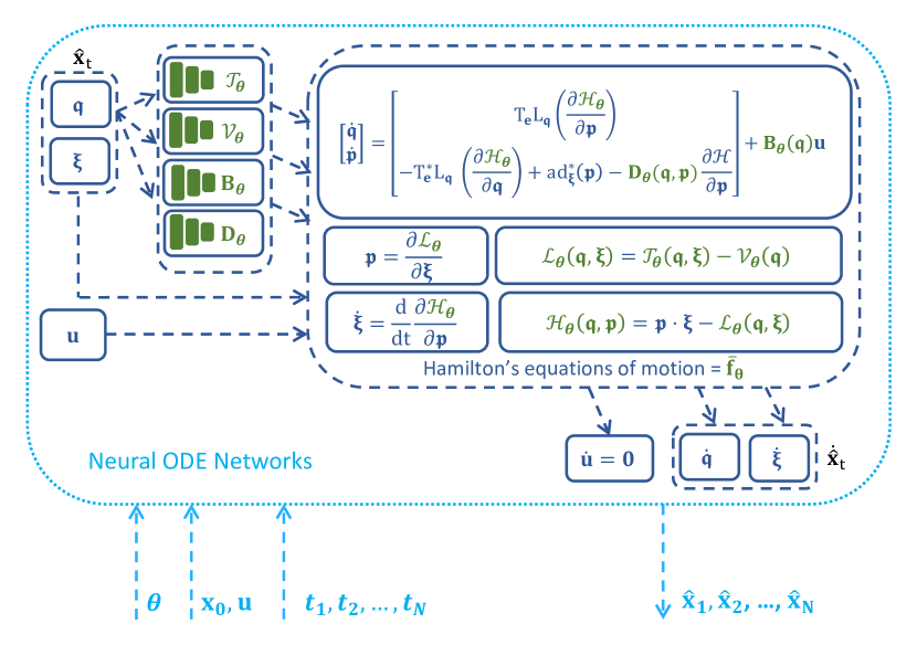
Figure 2: Architecture of port-Hamiltonian neural ODE network on a Lie group. The trainable terms are shown in green.

To integrate the Hamiltonian equations into the structure of $\bar{\mathbf{f}}_{\boldsymbol{\theta}}(\mathbf{x},\mathbf{u})$, we use four neural networks with parameters $\boldsymbol{\theta}=(\boldsymbol{\theta}_{{\cal T}},\boldsymbol{\theta}_{{\cal V}},\boldsymbol{\theta}_{\mathbf{D}},\boldsymbol{\theta}_{\mathbf{B}})$ to approximate the kinetic energy by ${\cal T}_{\boldsymbol{\theta}}({\boldsymbol{\mathfrak{q}}},\boldsymbol{\xi})$, the potential energy by ${\cal V}_{\boldsymbol{\theta}}({\boldsymbol{\mathfrak{q}}})$, the dissipation matrix by $\mathbf{D}_{\boldsymbol{\theta}}({\boldsymbol{\mathfrak{q}}},{\boldsymbol{\mathfrak{p}}})$, and the input matrix by $\mathbf{B}_{\boldsymbol{\theta}}({\boldsymbol{\mathfrak{q}}})$, respectively. Since the generalized momenta ${\boldsymbol{\mathfrak{p}}}$ are not directly available in ${\cal D}$, the time derivative of the generalized velocity $\boldsymbol{\xi}$ is obtained from Eq. (19). The approximated dynamics function $\bar{\mathbf{f}}_{\boldsymbol{\theta}}(\mathbf{x},\mathbf{u})$ is described with an internal state ${\boldsymbol{\mathfrak{p}}}$ as follows:

$$\dot{{\boldsymbol{\mathfrak{q}}}} =\mathsf{T}_{\mathbf{e}}\mathsf{L}_{\boldsymbol{\mathfrak{q}}}\left(\frac{\partial{\cal H}_{\boldsymbol{\theta}}({\boldsymbol{\mathfrak{q}}},{\boldsymbol{\mathfrak{p}}})}{\partial{\boldsymbol{\mathfrak{p}}}}\right),$$ (33a)

$$\dot{{\boldsymbol{\mathfrak{p}}}} =\mathsf{a}\mathsf{d}^{*}_{\boldsymbol{\xi}}({\boldsymbol{\mathfrak{p}}})-\mathbf{D}_{\boldsymbol{\theta}}({\boldsymbol{\mathfrak{q}}},{\boldsymbol{\mathfrak{p}}})\frac{\partial{\cal H}_{\boldsymbol{\theta}}({\boldsymbol{\mathfrak{q}}},{\boldsymbol{\mathfrak{p}}})}{\partial{\boldsymbol{\mathfrak{p}}}}$$

$$\qquad-\mathsf{T}_{\mathbf{e}}^{*}\mathsf{L}_{\boldsymbol{\mathfrak{q}}}\left(\frac{\partial{\cal H}_{\boldsymbol{\theta}}({\boldsymbol{\mathfrak{q}}},{\boldsymbol{\mathfrak{p}}})}{\partial{\boldsymbol{\mathfrak{q}}}}\right)+\mathbf{B}_{\boldsymbol{\theta}}({\boldsymbol{\mathfrak{q}}})\mathbf{u},$$ (33b)

$$\dot{\boldsymbol{\xi}} =\frac{d}{dt}\frac{\partial{\cal H}_{\boldsymbol{\theta}}({\boldsymbol{\mathfrak{q}}},{\boldsymbol{\mathfrak{p}}})}{\partial{\boldsymbol{\mathfrak{p}}}},$$ (33c)

where ${\cal H}_{\boldsymbol{\theta}}({\boldsymbol{\mathfrak{q}}},{\boldsymbol{\mathfrak{p}}})={\boldsymbol{\mathfrak{p}}}\cdot\boldsymbol{\xi}-{\cal L}_{\boldsymbol{\theta}}({\boldsymbol{\mathfrak{q}}},\boldsymbol{\xi})$, and ${\cal L}_{\boldsymbol{\theta}}({\boldsymbol{\mathfrak{q}}},\boldsymbol{\xi})={\cal T}_{\boldsymbol{\theta}}({\boldsymbol{\mathfrak{q}}},\boldsymbol{\xi})-{\cal V}_{\boldsymbol{\theta}}({\boldsymbol{\mathfrak{q}}})$. The time derivative $\frac{d}{dt}\frac{\partial{\cal H}_{\boldsymbol{\theta}}({\boldsymbol{\mathfrak{q}}},{\boldsymbol{\mathfrak{p}}})}{\partial{\boldsymbol{\mathfrak{p}}}}$ is calculated using automatic differentiation, e.g. by Pytorch [69]. The approximated dynamics function $\bar{\mathbf{f}}_{\boldsymbol{\theta}}(\mathbf{x},\mathbf{u})$ is implemented in a neural ODE network architecture for training, shown in Fig. 2.

V-C Training Process

Let $\bar{\mathbf{x}}^{(i)}(t)$ denote the state trajectory predicted with control input $\mathbf{u}^{(i)}$ by the approximate dynamics $\bar{\mathbf{f}}_{\boldsymbol{\theta}}$ initialized at $\bar{\mathbf{x}}^{(i)}(t_{0}^{(i)})=\mathbf{x}_{0}^{(i)}$. For sequence $i$, forward passes through the ODE solver in (31) return the predicted states $\bar{\mathbf{x}}^{(i)}_{0:N}$ at times $t^{(i)}_{0:N}$, where $\bar{\mathbf{x}}_{n}^{(i)}=[\bar{{\boldsymbol{\mathfrak{q}}}}_{n}^{(i)\top}\quad\bar{\boldsymbol{\xi}}_{n}^{(i)\top}]^{\top}$, for $n=1,\ldots,N$. The predicted coordinates $\bar{{\boldsymbol{\mathfrak{q}}}}_{n}^{(i)}$ and the ground-truth ones ${\boldsymbol{\mathfrak{q}}}_{n}^{(i)}$ are used to calculate a loss on the Lie group manifold:

$$L_{{\boldsymbol{\mathfrak{q}}}}(\boldsymbol{\theta})=\sum_{i=1}^{D}\sum_{n=1}^{N}\left\|\log_{\mathsf{G}}^{\vee}\left(\bar{{\boldsymbol{\mathfrak{q}}}}_{n}^{(i)}\left({\boldsymbol{\mathfrak{q}}}_{n}^{(i)}\right)^{-1}\right)\right\|_{2}^{2}.$$ (34)

We use the squared Euclidean norm to calculate losses for the generalized velocity terms:

$$L_{\boldsymbol{\xi}}(\boldsymbol{\theta})=\sum_{i=1}^{D}\sum_{n=1}^{N}\|\boldsymbol{\xi}_{n}^{(i)}-\bar{\boldsymbol{\xi}}_{n}^{(i)}\|^{2}_{2}.$$ (35)

The total loss $L(\boldsymbol{\theta})$ is defined as:

$$L(\boldsymbol{\theta})=L_{{\boldsymbol{\mathfrak{q}}}}(\boldsymbol{\theta})+L_{\boldsymbol{\xi}}(\boldsymbol{\theta}).$$ (36)

The gradient of the total loss function $L(\boldsymbol{\theta})$ is back-propagated by solving an ODE with adjoint states [28]. Specifically, let $\mathbf{a}=\frac{\partial L}{\partial\bar{\mathbf{x}}}$ be the adjoint state and $\mathbf{s}=(\bar{\mathbf{x}},\mathbf{a},\frac{\partial L}{\partial\boldsymbol{\theta}})$ be the augmented state. The augmented state dynamics are [28]:

$$\dot{\mathbf{s}}=\bar{\mathbf{f}}_{\mathbf{s}}=(\bar{\mathbf{f}}_{\boldsymbol{\theta}},-\mathbf{a}^{\top}\frac{\partial\bar{\mathbf{f}}_{\boldsymbol{\theta}}}{\partial\bar{\mathbf{x}}},-\mathbf{a}^{\top}\frac{\partial\bar{\mathbf{f}}_{\boldsymbol{\theta}}}{\partial\boldsymbol{\theta}}).$$ (37)

The predicted state $\bar{\mathbf{x}}$, the adjoint state $\mathbf{a}$, and the derivatives $\frac{\partial L}{\partial\boldsymbol{\theta}}$ can be obtained by a single call to a reverse-time ODE solver starting from $\mathbf{s}_{N}=\mathbf{s}({t_{N}})$:

$$\mathbf{s}_{0}=\left(\bar{\mathbf{x}}_{0},\mathbf{a}_{0},\frac{\partial{\cal L}}{\partial\boldsymbol{\theta}}\right)=\text{ODESolver}(\mathbf{s}_{N},\bar{\mathbf{f}}_{\mathbf{s}},t_{N}),$$ (38)

where at each time $t_{k},k=1,\ldots,N$, the adjoint state $\mathbf{a}_{k}$ at time $t_{k}$ is reset to $\frac{\partial L}{\partial\bar{\mathbf{x}}_{k}}$. The resulting derivative $\frac{\partial L}{\partial\boldsymbol{\theta}}$ is used to update the parameters $\boldsymbol{\theta}$ using gradient descent.

V-D Application to SE(3) Hamiltonian Dynamics Learning

This section applies our Lie group Hamiltonian dynamics learning approach to estimate mobile robot dynamics on the $SE(3)$ manifold (Sec. IV-E).

Neural ODE model architecture

When the Hamiltonian dynamics in (17) are defined on the $SE(3)$ manifold, the equations of motion become (30). The neural ODE network architecture in (33) is simplified as follows. We use five neural networks with parameters $\boldsymbol{\theta}=(\boldsymbol{\theta}_{\mathbf{v}},\boldsymbol{\theta}_{\boldsymbol{\omega}},\boldsymbol{\theta}_{V},\boldsymbol{\theta}_{\mathbf{D}},\boldsymbol{\theta}_{\mathbf{B}})$ to approximate the blocks $\mathbf{M}^{-1}_{\mathbf{v};{\boldsymbol{\theta}}}({\boldsymbol{\mathfrak{q}}})$, $\mathbf{M}^{-1}_{\boldsymbol{\omega};{\boldsymbol{\theta}}}({\boldsymbol{\mathfrak{q}}})$ of the inverse generalized mass in (25), the potential energy ${\cal V}_{\boldsymbol{\theta}}({\boldsymbol{\mathfrak{q}}})$, the dissipation matrix $\mathbf{D}_{\boldsymbol{\theta}}({\boldsymbol{\mathfrak{q}}},{\boldsymbol{\mathfrak{p}}})$, and the input matrix $\mathbf{B}_{\boldsymbol{\theta}}({\boldsymbol{\mathfrak{q}}})$, respectively. The approximated kinetic energy is calculated as ${\cal T}_{\boldsymbol{\theta}}({\boldsymbol{\mathfrak{q}}},{\boldsymbol{\mathfrak{p}}})=\frac{1}{2}{\boldsymbol{\mathfrak{p}}}^{\top}\mathbf{M}^{-1}_{\boldsymbol{\theta}}({\boldsymbol{\mathfrak{q}}}){\boldsymbol{\mathfrak{p}}}$, where $\mathbf{M}_{\boldsymbol{\theta}}({\boldsymbol{\mathfrak{q}}})=\operatorname{diag}(\mathbf{M}_{\mathbf{v};{\boldsymbol{\theta}}}({\boldsymbol{\mathfrak{q}}}),\mathbf{M}_{\boldsymbol{\omega};{\boldsymbol{\theta}}}({\boldsymbol{\mathfrak{q}}}))$.

Neural network design

In many applications, nominal information is available about the generalized mass matrices $\mathbf{M}^{-1}_{\mathbf{v};{\boldsymbol{\theta}}}({\boldsymbol{\mathfrak{q}}})$, $\mathbf{M}^{-1}_{\boldsymbol{\omega};{\boldsymbol{\theta}}}({\boldsymbol{\mathfrak{q}}})$, the potential energy ${\cal V}_{\boldsymbol{\theta}}({\boldsymbol{\mathfrak{q}}})$, the dissipation matrix $\mathbf{D}_{\boldsymbol{\theta}}({\boldsymbol{\mathfrak{q}}},{\boldsymbol{\mathfrak{p}}})$, and the input matrix $\mathbf{B}_{\boldsymbol{\theta}}({\boldsymbol{\mathfrak{q}}})$, and can be included in the neural network design.

Let $\mathbf{M}^{-1}_{\mathbf{v}0}({\boldsymbol{\mathfrak{q}}})$, $\mathbf{M}^{-1}_{\boldsymbol{\omega}0}({\boldsymbol{\mathfrak{q}}})$, and $\mathbf{D}_{0}({\boldsymbol{\mathfrak{q}}},{\boldsymbol{\mathfrak{p}}})$ be the nominal values of the generalized mass matrices $\mathbf{M}^{-1}_{\mathbf{v};\boldsymbol{\theta}}({\boldsymbol{\mathfrak{q}}})$, $\mathbf{M}^{-1}_{\boldsymbol{\omega};\boldsymbol{\theta}}({\boldsymbol{\mathfrak{q}}})$ and the dissipation matrix $\mathbf{D}_{\boldsymbol{\theta}}({\boldsymbol{\mathfrak{q}}},{\boldsymbol{\mathfrak{p}}})$ with Cholesky decomposition:

$$\mathbf{M}^{-1}_{\mathbf{v}0}({\boldsymbol{\mathfrak{q}}}) =\mathbf{L}_{\mathbf{v}0}({\boldsymbol{\mathfrak{q}}})\mathbf{L}^{\top}_{\mathbf{v}0}({\boldsymbol{\mathfrak{q}}}),$$ (39)

$$\mathbf{M}^{-1}_{\boldsymbol{\omega}0}({\boldsymbol{\mathfrak{q}}}) =\mathbf{L}_{\boldsymbol{\omega}0}({\boldsymbol{\mathfrak{q}}})\mathbf{L}^{\top}_{\boldsymbol{\omega}0}({\boldsymbol{\mathfrak{q}}}),$$

$$\mathbf{D}_{0}({\boldsymbol{\mathfrak{q}}}) =\mathbf{L}_{\mathbf{D}0}({\boldsymbol{\mathfrak{q}}})\mathbf{L}^{\top}_{\mathbf{D}0}({\boldsymbol{\mathfrak{q}}}).$$

The learned terms $\mathbf{M}^{-1}_{\mathbf{v};{\boldsymbol{\theta}}}({\boldsymbol{\mathfrak{q}}})$, $\mathbf{M}^{-1}_{\boldsymbol{\omega};{\boldsymbol{\theta}}}({\boldsymbol{\mathfrak{q}}})$, and $\mathbf{D}_{\boldsymbol{\theta}}({\boldsymbol{\mathfrak{q}}},{\boldsymbol{\mathfrak{p}}})$ are obtained using Cholesky decomposition:

$$\mathbf{M}^{-1}_{\mathbf{v};{\boldsymbol{\theta}}}({\boldsymbol{\mathfrak{q}}}) =\left(\mathbf{L}_{\mathbf{v}0}({\boldsymbol{\mathfrak{q}}})+\mathbf{L}_{\mathbf{v}}({\boldsymbol{\mathfrak{q}}})\right)\left(\mathbf{L}_{\mathbf{v}0}({\boldsymbol{\mathfrak{q}}})+\mathbf{L}_{\mathbf{v}}({\boldsymbol{\mathfrak{q}}})\right)^{\top}+\varepsilon_{\mathbf{v}}\mathbf{I},$$ (40)

$$\mathbf{M}^{-1}_{\boldsymbol{\omega};{\boldsymbol{\theta}}}({\boldsymbol{\mathfrak{q}}}) =\left(\mathbf{L}_{\boldsymbol{\omega}0}({\boldsymbol{\mathfrak{q}}})+\mathbf{L}_{\boldsymbol{\omega}}({\boldsymbol{\mathfrak{q}}})\right)\left(\mathbf{L}_{\boldsymbol{\omega}0}({\boldsymbol{\mathfrak{q}}})+\mathbf{L}_{\boldsymbol{\omega}}({\boldsymbol{\mathfrak{q}}})\right)^{\top}+\varepsilon_{\boldsymbol{\omega}}\mathbf{I},$$

$$\mathbf{D}_{\boldsymbol{\theta}}({\boldsymbol{\mathfrak{q}}},{\boldsymbol{\mathfrak{p}}}) =\left(\mathbf{L}_{\mathbf{D}0}({\boldsymbol{\mathfrak{q}}},{\boldsymbol{\mathfrak{p}}})\!+\!\mathbf{L}_{\mathbf{D}}({\boldsymbol{\mathfrak{q}}},{\boldsymbol{\mathfrak{p}}})\right)\left(\mathbf{L}_{\mathbf{D}0}({\boldsymbol{\mathfrak{q}}},{\boldsymbol{\mathfrak{p}}})\!+\!\mathbf{L}_{D}({\boldsymbol{\mathfrak{q}}},{\boldsymbol{\mathfrak{p}}})\right)^{\top}$$

where $\mathbf{L}_{{}_{\mathbf{v}}}({\boldsymbol{\mathfrak{q}}})$, $\mathbf{L}_{\boldsymbol{\omega}}({\boldsymbol{\mathfrak{q}}})$, and $\mathbf{L}_{\mathbf{D}}({\boldsymbol{\mathfrak{q}}},{\boldsymbol{\mathfrak{p}}})$ are lower-triangular matrices implemented as three neural networks with parameters $\boldsymbol{\theta}_{\mathbf{v}}$, $\boldsymbol{\theta}_{\boldsymbol{\omega}}$, and $\boldsymbol{\theta}_{\mathbf{D}}$ respectively, and $\varepsilon_{\mathbf{v}},\varepsilon_{\boldsymbol{\omega}}>0$.

The potential energy ${\cal V}({\boldsymbol{\mathfrak{q}}})$ and the input matrix $\mathbf{B}({\boldsymbol{\mathfrak{q}}})$ are implemented with nominal values ${\cal V}_{0}({\boldsymbol{\mathfrak{q}}})$ and $\mathbf{B}_{0}({\boldsymbol{\mathfrak{q}}})$ as follows:

$${\cal V}_{\boldsymbol{\theta}}({\boldsymbol{\mathfrak{q}}}) ={\cal V}_{0}({\boldsymbol{\mathfrak{q}}})+\text{L}_{{\cal V}}({\boldsymbol{\mathfrak{q}}}),$$ (41)

$$\mathbf{B}_{\boldsymbol{\theta}}({\boldsymbol{\mathfrak{q}}}) =\mathbf{B}_{0}({\boldsymbol{\mathfrak{q}}})+\mathbf{L}_{\mathbf{B}}({\boldsymbol{\mathfrak{q}}}),$$

where $\text{L}_{\cal V}({\boldsymbol{\mathfrak{q}}})$ and $\mathbf{L}_{\mathbf{B}}({\boldsymbol{\mathfrak{q}}})$ are two neural networks with parameters $\boldsymbol{\theta}_{\cal V}$ and $\boldsymbol{\theta}_{\mathbf{B}}$, respectively.

Loss function

The orientation loss is calculated as:

$$L_{\mathbf{R}}(\boldsymbol{\theta})=\sum_{i=1}^{D}\sum_{n=1}^{N}\left\|\log_{SO(3)}^{\vee}(\bar{\mathbf{R}}_{n}^{(i)}\mathbf{R}_{n}^{(i)\top})\right\|_{2}^{2},$$ (42)

We use the squared Euclidean norm to calculate losses for the position and generalized velocity terms:

$$L_{\mathbf{p}}(\boldsymbol{\theta}) = \sum_{i=1}^{D}\sum_{n=1}^{N}\|\mathbf{p}_{n}^{(i)}-\bar{\mathbf{p}}_{n}^{(i)}\|^{2}_{2},$$ (43)

$$L_{\boldsymbol{\zeta}}(\boldsymbol{\theta}) = \sum_{i=1}^{D}\sum_{n=1}^{N}\|\boldsymbol{\zeta}_{n}^{(i)}-\bar{\boldsymbol{\zeta}}_{n}^{(i)}\|^{2}_{2}.$$

The total loss ${\cal L}(\boldsymbol{\theta})$ is defined as:

$$L(\boldsymbol{\theta})=L_{\mathbf{R}}(\boldsymbol{\theta})+L_{\mathbf{p}}(\boldsymbol{\theta})+L_{\boldsymbol{\zeta}}(\boldsymbol{\theta}).$$ (44)

VI Energy-based Control Design

The function $\bar{\mathbf{f}}_{\boldsymbol{\theta}}$ (33) learned in Sec. V satisfies the port-Hamiltonian dynamics in Eq. (22) by design. This section extends the interconnection and damping assignment passivity-based control (IDA-PBC) approach [31, 57, 58] to Lie groups to achieve trajectory tracking (Problem 2) based on the learned port-Hamiltonian dynamics. We further derive a tracking controller specifically for learned Hamiltonian dynamics on the $SE(3)$ manifold in Sec. V-D. In the remainder of the paper, we omit the subscript $\boldsymbol{\theta}$ in the learned model for readability.

VI-A IDA-PBC Control Design for Trajectory Tracking

Consider a desired regulation point $({\boldsymbol{\mathfrak{q}}}^{*},{\boldsymbol{\mathfrak{p}}}^{*})\in\mathsf{T}^{*}\mathsf{G}$ that the system should be stabilized to. The Hamiltonian function $\mathcal{H}({\boldsymbol{\mathfrak{q}}},{\boldsymbol{\mathfrak{p}}})$, representing the total energy of the system, generally does not have a minimum at $({\boldsymbol{\mathfrak{q}}}^{*},{\boldsymbol{\mathfrak{p}}}^{*})$. An IDA-PBC controller [31, 54, 57] is designed to inject additional energy ${\cal H}_{a}({\boldsymbol{\mathfrak{q}}},{\boldsymbol{\mathfrak{p}}})$ such that the desired total energy:

$$\mathcal{H}_{d}({\boldsymbol{\mathfrak{q}}},{\boldsymbol{\mathfrak{p}}})=\mathcal{H}({\boldsymbol{\mathfrak{q}}},{\boldsymbol{\mathfrak{p}}})+\mathcal{H}_{a}({\boldsymbol{\mathfrak{q}}},{\boldsymbol{\mathfrak{p}}})$$ (45)

achieves its minimum at $({\boldsymbol{\mathfrak{q}}}^{*},{\boldsymbol{\mathfrak{p}}}^{*})$. In other words, the closed-loop system obtained by applying the controller to the port-Hamiltonian dynamics in (22) should have the form:

$$\begin{bmatrix}\dot{{\boldsymbol{\mathfrak{q}}}}\\ \dot{{\boldsymbol{\mathfrak{p}}}}\\ \end{bmatrix}=(\mathcal{J}_{d}({\boldsymbol{\mathfrak{q}}},{\boldsymbol{\mathfrak{p}}})-\mathcal{R}_{d}({\boldsymbol{\mathfrak{q}}},{\boldsymbol{\mathfrak{p}}}))\begin{bmatrix}\frac{\partial\mathcal{H}_{d}}{\partial{\boldsymbol{\mathfrak{q}}}}\\ \frac{\partial\mathcal{H}_{d}}{\partial{\boldsymbol{\mathfrak{p}}}}\end{bmatrix}.$$ (46)

to ensure that $({\boldsymbol{\mathfrak{q}}}^{*},{\boldsymbol{\mathfrak{p}}}^{*})$ is an equilibrium. The control input $\mathbf{u}$ should be chosen so that (22) and (46) are equal. This matching equation design does not directly apply to trajectory tracking, especially for underactuated systems [58, 57].

Consider a desired trajectory $({\boldsymbol{\mathfrak{q}}}^{*}(t),{\boldsymbol{\mathfrak{p}}}^{*}(t))$ that the system should track. Let $({\boldsymbol{\mathfrak{q}}}_{e}(t),{\boldsymbol{\mathfrak{p}}}_{e}(t))$ denote the error in the generalized coordinates and momentum, respectively, where ${\boldsymbol{\mathfrak{q}}}_{e}=({\boldsymbol{\mathfrak{q}}}^{*})^{-1}{\boldsymbol{\mathfrak{q}}}\in\mathsf{G}$ and ${\boldsymbol{\mathfrak{p}}}_{e}={\boldsymbol{\mathfrak{p}}}-{\boldsymbol{\mathfrak{p}}}^{*}\in\mathsf{T}_{{\boldsymbol{\mathfrak{q}}}_{e}}^{*}\mathsf{G}$. For trajectory tracking, the desired total energy ${\cal H}_{d}({\boldsymbol{\mathfrak{q}}}_{e},{\boldsymbol{\mathfrak{p}}}_{e})$ is defined in terms of the error state, with desired closed-loop dynamics:

$$\begin{bmatrix}\dot{{\boldsymbol{\mathfrak{q}}}}_{e}\\ \dot{{\boldsymbol{\mathfrak{p}}}}_{e}\\ \end{bmatrix}=(\mathcal{J}_{d}({\boldsymbol{\mathfrak{q}}}_{e},{\boldsymbol{\mathfrak{p}}}_{e})-\mathcal{R}_{d}({\boldsymbol{\mathfrak{q}}}_{e},{\boldsymbol{\mathfrak{p}}}_{e}))\begin{bmatrix}\frac{\partial\mathcal{H}_{d}}{\partial{\boldsymbol{\mathfrak{q}}}_{e}}\\ \frac{\partial\mathcal{H}_{d}}{\partial{\boldsymbol{\mathfrak{p}}}_{e}}\end{bmatrix}.$$ (47)

Matching (47) with (22) leads to the following requirement for the control input:

$$\mathbf{{\cal G}}({\boldsymbol{\mathfrak{q}}},{\boldsymbol{\mathfrak{p}}})\mathbf{u}=( \mathcal{J}_{d}({\boldsymbol{\mathfrak{q}}}_{e},{\boldsymbol{\mathfrak{p}}}_{e})-\mathcal{R}_{d}({\boldsymbol{\mathfrak{q}}}_{e},{\boldsymbol{\mathfrak{p}}}_{e}))\begin{bmatrix}\frac{\partial\mathcal{H}_{d}}{\partial{\boldsymbol{\mathfrak{q}}}_{e}}\\ \frac{\partial\mathcal{H}_{d}}{\partial{\boldsymbol{\mathfrak{p}}}_{e}}\end{bmatrix}$$ (48)

$$-( \mathbf{{\cal J}}({\boldsymbol{\mathfrak{q}}},{\boldsymbol{\mathfrak{p}}})-\mathbf{{\cal R}}({\boldsymbol{\mathfrak{q}}},{\boldsymbol{\mathfrak{p}}}))\begin{bmatrix}\frac{\partial\mathcal{H}}{\partial{\boldsymbol{\mathfrak{q}}}}\\ \frac{\partial\mathcal{H}}{\partial{\boldsymbol{\mathfrak{p}}}}\end{bmatrix}+\begin{bmatrix}\dot{{\boldsymbol{\mathfrak{q}}}}\\ \dot{{\boldsymbol{\mathfrak{p}}}}\end{bmatrix}-\begin{bmatrix}\dot{{\boldsymbol{\mathfrak{q}}}}_{e}\\ \dot{{\boldsymbol{\mathfrak{p}}}}_{e}\end{bmatrix}.$$

The control input can be obtained from (48) as the sum $\mathbf{u}=\mathbf{u}_{ES}+\mathbf{u}_{DI}$ of an energy-shaping component $\mathbf{u}_{ES}$ and a damping-injection component $\mathbf{u}_{DI}$:

$$\mathbf{u}_{ES} =\mathbf{{\cal G}}^{\dagger}({\boldsymbol{\mathfrak{q}}},{\boldsymbol{\mathfrak{p}}})\left((\mathcal{J}_{d}({\boldsymbol{\mathfrak{q}}}_{e},{\boldsymbol{\mathfrak{p}}}_{e}))\begin{bmatrix}\frac{\partial\mathcal{H}_{d}}{\partial{\boldsymbol{\mathfrak{q}}}_{e}}\\ \frac{\partial\mathcal{H}_{d}}{\partial{\boldsymbol{\mathfrak{p}}}_{e}}\end{bmatrix}-\begin{bmatrix}\dot{{\boldsymbol{\mathfrak{q}}}}_{e}\\ \dot{{\boldsymbol{\mathfrak{p}}}}_{e}\end{bmatrix}\right.$$ (49a)

$$\left.\qquad-(\mathbf{{\cal J}}({\boldsymbol{\mathfrak{q}}},{\boldsymbol{\mathfrak{p}}})-\mathbf{{\cal R}}({\boldsymbol{\mathfrak{q}}},{\boldsymbol{\mathfrak{p}}}))\begin{bmatrix}\frac{\partial\mathcal{H}}{\partial{\boldsymbol{\mathfrak{q}}}}\\ \frac{\partial\mathcal{H}}{\partial{\boldsymbol{\mathfrak{p}}}}\end{bmatrix}+\begin{bmatrix}\dot{{\boldsymbol{\mathfrak{q}}}}\\ \dot{{\boldsymbol{\mathfrak{p}}}}\end{bmatrix}\right),$$

$$\mathbf{u}_{DI} =-\mathbf{{\cal G}}^{\dagger}({\boldsymbol{\mathfrak{q}}},{\boldsymbol{\mathfrak{p}}})\mathcal{R}_{d}({\boldsymbol{\mathfrak{q}}}_{e},{\boldsymbol{\mathfrak{p}}}_{e})\begin{bmatrix}\frac{\partial\mathcal{H}_{d}}{\partial{\boldsymbol{\mathfrak{q}}}_{e}}\\ \frac{\partial\mathcal{H}_{d}}{\partial{\boldsymbol{\mathfrak{p}}}_{e}}\end{bmatrix},$$ (49b)

where $\mathbf{{\cal G}}^{\dagger}({\boldsymbol{\mathfrak{q}}},{\boldsymbol{\mathfrak{p}}})=\left(\mathbf{{\cal G}}^{\top}({\boldsymbol{\mathfrak{q}}},{\boldsymbol{\mathfrak{p}}})\mathbf{{\cal G}}({\boldsymbol{\mathfrak{q}}},{\boldsymbol{\mathfrak{p}}})\right)^{-1}\mathbf{{\cal G}}^{\top}({\boldsymbol{\mathfrak{q}}},{\boldsymbol{\mathfrak{p}}})$ is the pseudo-inverse of $\mathbf{{\cal G}}({\boldsymbol{\mathfrak{q}}},{\boldsymbol{\mathfrak{p}}})$. The control input $\mathbf{u}_{ES}$ exists as long as the desired interconnection matrix $\mathcal{J}_{d}$, dissipation matrix $\mathcal{R}_{d}$, and total energy $\mathcal{H}_{d}$ satisfy the following matching condition for all $({\boldsymbol{\mathfrak{q}}},{\boldsymbol{\mathfrak{p}}})\in\mathsf{T}^{*}\mathsf{G}$ and $({\boldsymbol{\mathfrak{q}}}_{e},{\boldsymbol{\mathfrak{p}}}_{e})\in\mathsf{T}^{*}\mathsf{G}$:

$${\cal G}^{\dagger}({\boldsymbol{\mathfrak{q}}},{\boldsymbol{\mathfrak{p}}}) \left(\mathcal{J}_{d}({\boldsymbol{\mathfrak{q}}}_{e},{\boldsymbol{\mathfrak{p}}}_{e})-\mathcal{R}_{d}({\boldsymbol{\mathfrak{q}}}_{e},{\boldsymbol{\mathfrak{p}}}_{e}))\begin{bmatrix}\frac{\partial\mathcal{H}_{d}}{\partial{\boldsymbol{\mathfrak{q}}}_{e}}\\ \frac{\partial\mathcal{H}_{d}}{\partial{\boldsymbol{\mathfrak{p}}}_{e}}\end{bmatrix}\right.$$ (50)

$$- \left.({\cal J}({\boldsymbol{\mathfrak{q}}},{\boldsymbol{\mathfrak{p}}})-{\cal R}({\boldsymbol{\mathfrak{q}}},{\boldsymbol{\mathfrak{p}}}))\begin{bmatrix}\frac{\partial\mathcal{H}}{\partial{\boldsymbol{\mathfrak{q}}}}\\ \frac{\partial\mathcal{H}}{\partial{\boldsymbol{\mathfrak{p}}}}\end{bmatrix}+\begin{bmatrix}\dot{{\boldsymbol{\mathfrak{q}}}}\\ \dot{{\boldsymbol{\mathfrak{p}}}}\end{bmatrix}-\begin{bmatrix}\dot{{\boldsymbol{\mathfrak{q}}}}_{e}\\ \dot{{\boldsymbol{\mathfrak{p}}}}_{e}\end{bmatrix}\right)=0.$$

where ${\cal G}^{\perp}({\boldsymbol{\mathfrak{q}}},{\boldsymbol{\mathfrak{p}}})$ is a maximal-rank left annihilator of ${\cal G}({\boldsymbol{\mathfrak{q}}},{\boldsymbol{\mathfrak{p}}})$, i.e., ${\cal G}^{\perp}({\boldsymbol{\mathfrak{q}}},{\boldsymbol{\mathfrak{p}}}){\cal G}({\boldsymbol{\mathfrak{q}}},{\boldsymbol{\mathfrak{p}}})=\bf 0$.

VI-B Tracking Control for Port-Hamiltonian Dynamics on the SE(3) Manifold

Consider a desired state trajectory $\mathbf{x}^{*}(t)=({\boldsymbol{\mathfrak{q}}}^{*}(t),\boldsymbol{\zeta}^{*}(t))$ that the system should track where ${\boldsymbol{\mathfrak{q}}}^{*}(t)\in SE(3)$ is the desired pose and $\boldsymbol{\zeta}^{*}(t)=\begin{bmatrix}\mathbf{v}^{*}(t)^{\top}&\boldsymbol{\omega}^{*}(t)^{\top}\end{bmatrix}^{\top}$ is the desired generalized velocity expressed in the desired frame. Let ${\boldsymbol{\mathfrak{p}}}^{*}=\mathbf{M}\begin{bmatrix}\mathbf{R}^{\top}\mathbf{R}^{*}\mathbf{v}^{*}\\ \mathbf{R}^{\top}\mathbf{R}^{*}\boldsymbol{\omega}^{*}\end{bmatrix}$ denote the desired momentum, defined based on (26) with the desired velocity expressed in the body frame. Let $\mathbf{p}_{e}=\mathbf{p}-\mathbf{p}^{*}$ and $\mathbf{R}_{e}=\mathbf{R}^{*\top}\mathbf{R}=\begin{bmatrix}\mathbf{r}_{e1}&\mathbf{r}_{e2}&\mathbf{r}_{e3}\end{bmatrix}^{\top}$ be the position error and rotation error between the current orientation $\mathbf{R}$ and the desired one $\mathbf{R}^{*}$, respectively. The vectorized error ${\boldsymbol{\mathfrak{q}}}_{e}$ in the generalized coordinates is:

$${\boldsymbol{\mathfrak{q}}}_{e}=\begin{bmatrix}\mathbf{p}_{e}^{*\top}&\mathbf{r}_{e1}^{\top}&\mathbf{r}_{e2}^{\top}&\mathbf{r}_{e3}^{\top}\end{bmatrix}^{\top}.$$ (51)

The error in the generalized momenta is ${\boldsymbol{\mathfrak{p}}}_{e}={\boldsymbol{\mathfrak{p}}}-{\boldsymbol{\mathfrak{p}}}^{*}$, described in the body frame. The desired total energy is defined in terms of the error state as:

$${\cal H}_{d}({\boldsymbol{\mathfrak{q}}}_{e},{\boldsymbol{\mathfrak{p}}}_{e})=\frac{1}{2}{\boldsymbol{\mathfrak{p}}}_{e}^{\top}\mathbf{M}_{d}^{-1}({\boldsymbol{\mathfrak{q}}}_{e}){\boldsymbol{\mathfrak{p}}}_{e}+V_{d}({\boldsymbol{\mathfrak{q}}}_{e}),$$ (52)

where $\mathbf{M}_{d}({\boldsymbol{\mathfrak{q}}}_{e})$ and $V_{d}({\boldsymbol{\mathfrak{q}}}_{e})$ are the desired generalized mass and potential energy. Choosing the following desired inter-connection matrix and dissipation matrix:

$$\mathcal{J}_{d}({\boldsymbol{\mathfrak{q}}}_{e},{\boldsymbol{\mathfrak{p}}}_{e})=\begin{bmatrix}\bf 0&\mathbf{J}_{1}\\ -\mathbf{J}_{1}^{\top}&\mathbf{J}_{2}\end{bmatrix},\quad\mathcal{R}_{d}({\boldsymbol{\mathfrak{q}}}_{e},{\boldsymbol{\mathfrak{p}}}_{e})=\begin{bmatrix}\bf 0&\bf 0\\ \bf 0&\mathbf{K}_{\mathbf{d}}\end{bmatrix},$$ (53)

and plugging ${\cal J}({\boldsymbol{\mathfrak{q}}},{\boldsymbol{\mathfrak{p}}})$ and ${\cal R}({\boldsymbol{\mathfrak{q}}},{\boldsymbol{\mathfrak{p}}})$ from (28) into the matching equations in (48), leads to:

$$\bf 0 = \mathbf{J}_{1}\frac{\partial{\cal H}_{d}}{\partial{\boldsymbol{\mathfrak{p}}}_{e}}-{\boldsymbol{\mathfrak{q}}}^{\times}\frac{\partial{\cal H}}{\partial{\boldsymbol{\mathfrak{p}}}}+\dot{{\boldsymbol{\mathfrak{q}}}}-\dot{{\boldsymbol{\mathfrak{q}}}}_{e},$$ (54)

$$\mathbf{B}({\boldsymbol{\mathfrak{q}}})\mathbf{u} = {\boldsymbol{\mathfrak{q}}}^{\times\top}\frac{\partial{\cal H}}{\partial{\boldsymbol{\mathfrak{q}}}}-\mathbf{J}_{1}^{\top}\frac{\partial{\cal H}_{d}}{\partial{\boldsymbol{\mathfrak{q}}}_{e}}+\mathbf{J}_{2}\frac{\partial{\cal H}_{d}}{\partial{\boldsymbol{\mathfrak{p}}}_{e}}-{\boldsymbol{\mathfrak{p}}}^{\times}\frac{\partial{\cal H}}{\partial{\boldsymbol{\mathfrak{p}}}}$$ (55)

$$-\mathbf{K}_{\mathbf{d}}\frac{\partial{\cal H}_{d}}{\partial{\boldsymbol{\mathfrak{p}}}_{e}}+\mathbf{D}({\boldsymbol{\mathfrak{q}}},{\boldsymbol{\mathfrak{p}}})\frac{\partial{\cal H}}{\partial{\boldsymbol{\mathfrak{p}}}}+\dot{{\boldsymbol{\mathfrak{p}}}}-\dot{{\boldsymbol{\mathfrak{p}}}}_{e}.$$

Assuming $\mathbf{M}_{d}({\boldsymbol{\mathfrak{q}}}_{e})=\mathbf{M}({\boldsymbol{\mathfrak{q}}})$, (54) is satisfied if we choose $\mathbf{J}_{1}=\begin{bmatrix}\mathbf{R}^{\top}\!\!\!\!&\bf 0&\bf 0&\bf 0\\ \bf 0&\hat{\mathbf{r}}_{e1}^{\top}&\hat{\mathbf{r}}_{e2}^{\top}&\hat{\mathbf{r}}_{e3}^{\top}\end{bmatrix}^{\top}$. Indeed, we have $\dot{{\boldsymbol{\mathfrak{q}}}}={\boldsymbol{\mathfrak{q}}}^{\times}\frac{\partial{\cal H}}{\partial{\boldsymbol{\mathfrak{p}}}}$ (from (11) and (19)) and

$$\frac{\partial{\cal H}_{d}}{\partial{\boldsymbol{\mathfrak{p}}}_{e}}=\mathbf{M}^{-1}_{d}{\boldsymbol{\mathfrak{p}}}_{e}=\begin{bmatrix}\mathbf{v}_{e}\\ \boldsymbol{\omega}_{e}\end{bmatrix}=\begin{bmatrix}\mathbf{v}-\mathbf{R}^{\top}\mathbf{R}^{*}\mathbf{v}^{*}\\ \boldsymbol{\omega}-\mathbf{R}^{\top}\mathbf{R}^{*}\boldsymbol{\omega}^{*}\end{bmatrix}.$$

The error dynamics becomes:

$$\dot{{\boldsymbol{\mathfrak{q}}}}_{e}=\begin{bmatrix}\dot{\mathbf{p}}-\dot{\mathbf{p}}^{*}\\ \dot{\mathbf{r}}_{e1}\\ \dot{\mathbf{r}}_{e2}\\ \dot{\mathbf{r}}_{e3}\end{bmatrix}=\begin{bmatrix}\mathbf{R}^{\top}\!\!\!\!&\bf 0&\bf 0&\bf 0\\ \bf 0&\hat{\mathbf{r}}_{e1}^{\top}&\hat{\mathbf{r}}_{e2}^{\top}&\hat{\mathbf{r}}_{e3}^{\top}\end{bmatrix}^{\top}\begin{bmatrix}\mathbf{v}_{e}\\ \boldsymbol{\omega}_{e}\end{bmatrix}=\mathbf{J}_{1}\frac{\partial{\cal H}_{d}}{\partial{\boldsymbol{\mathfrak{p}}}_{e}},$$ (56)

since $\dot{\mathbf{R}}_{e}=\frac{d}{dt}(\mathbf{R}_{e})=\mathbf{R}_{e}\widehat{\boldsymbol{\omega}}_{e}$ as shown in [70, Sec. III-A] and $\dot{\mathbf{p}}-\dot{\mathbf{p}}^{*}~{}=~{}\mathbf{R}\mathbf{v}-\mathbf{R}^{*}\mathbf{v}^{*}=\mathbf{R}\mathbf{v}_{e}$.

The desired control input can be obtained from (55) as $\mathbf{u}=\mathbf{u}_{ES}+\mathbf{u}_{DI}$ with:

$$\mathbf{u}_{ES} =\mathbf{B}^{\dagger}({\boldsymbol{\mathfrak{q}}})\left({\boldsymbol{\mathfrak{q}}}^{\times\top}\frac{\partial{\cal H}}{\partial{\boldsymbol{\mathfrak{q}}}}-\mathbf{\mathbf{J}}_{1}^{\top}\frac{\partial{\cal H}_{d}}{\partial{\boldsymbol{\mathfrak{q}}}_{e}}+\mathbf{J}_{2}\frac{\partial{\cal H}_{d}}{\partial{\boldsymbol{\mathfrak{p}}}_{e}}\right.$$ (57a)

$$\left.\qquad-{\boldsymbol{\mathfrak{p}}}^{\times}\frac{\partial{\cal H}}{\partial{\boldsymbol{\mathfrak{p}}}}+\mathbf{D}({\boldsymbol{\mathfrak{q}}},{\boldsymbol{\mathfrak{p}}})\frac{\partial{\cal H}}{\partial{\boldsymbol{\mathfrak{p}}}}+\dot{{\boldsymbol{\mathfrak{p}}}}-\dot{{\boldsymbol{\mathfrak{p}}}}_{e}\right),$$

$$\mathbf{u}_{DI} =-\mathbf{B}^{\dagger}({\boldsymbol{\mathfrak{q}}})\mathbf{K}_{\mathbf{d}}\frac{\partial{\cal H}_{d}}{\partial{\boldsymbol{\mathfrak{p}}}_{e}},$$ (57b)

where $\mathbf{B}^{\dagger}({\boldsymbol{\mathfrak{q}}})=\left(\mathbf{B}^{\top}({\boldsymbol{\mathfrak{q}}})\mathbf{B}({\boldsymbol{\mathfrak{q}}})\right)^{-1}\mathbf{B}^{\top}({\boldsymbol{\mathfrak{q}}})$ is the pseudo-inverse of $\mathbf{B}({\boldsymbol{\mathfrak{q}}})$. The matching condition (50) becomes:

$$\mathbf{B}^{\perp}({\boldsymbol{\mathfrak{q}}})\left({\boldsymbol{\mathfrak{q}}}^{\times\top}\frac{\partial{\cal H}}{\partial{\boldsymbol{\mathfrak{q}}}}-\mathbf{J}_{1}^{\top}\frac{\partial{\cal H}_{d}}{\partial{\boldsymbol{\mathfrak{q}}}_{e}}+\mathbf{J}_{2}\frac{\partial{\cal H}_{d}}{\partial{\boldsymbol{\mathfrak{p}}}_{e}}\right.$$ (58)

$$-\left.{\boldsymbol{\mathfrak{p}}}^{\times}\frac{\partial{\cal H}}{\partial{\boldsymbol{\mathfrak{p}}}}+\dot{{\boldsymbol{\mathfrak{p}}}}-\dot{{\boldsymbol{\mathfrak{p}}}}_{e}\right) =0.$$

In this paper, we reshape the open-loop Hamiltonian $\mathcal{H}({\boldsymbol{\mathfrak{q}}},{\boldsymbol{\mathfrak{p}}})$ into the following desired total energy $\mathcal{H}_{d}({\boldsymbol{\mathfrak{q}}}_{e},{\boldsymbol{\mathfrak{p}}}_{e})$, minimized along the desired trajectory:

$$\mathcal{H}_{d} ({\boldsymbol{\mathfrak{q}}}_{e},{\boldsymbol{\mathfrak{p}}}_{e})=\frac{1}{2}(\mathbf{p}-\mathbf{p}^{*})^{\top}\mathbf{K}_{\mathbf{p}}(\mathbf{p}-\mathbf{p}^{*})$$ (59)

$$+\frac{1}{2}\operatorname{tr}(\mathbf{K}_{\mathbf{R}}(\mathbf{I}-\mathbf{R}^{*\top}\mathbf{R}))+\frac{1}{2}({\boldsymbol{\mathfrak{p}}}-{\boldsymbol{\mathfrak{p}}}^{*})^{\top}\mathbf{M}^{-1}({\boldsymbol{\mathfrak{q}}})({\boldsymbol{\mathfrak{p}}}-{\boldsymbol{\mathfrak{p}}}^{*}),$$

where $\mathbf{K}_{\mathbf{p}},\mathbf{K}_{\mathbf{R}}\succ 0$ are positive-definite matrices.

For an $SE(3)$ rigid-body system with constant generalized mass matrix $\mathbf{M}_{d}=\mathbf{M}$ and $\mathbf{J}_{2}=0$, which is a common choice, the energy-shaping term in (57a) and the damping-injection term in (57b) simplify as:

$$\mathbf{u}_{ES}({\boldsymbol{\mathfrak{q}}},{\boldsymbol{\mathfrak{p}}}) =\mathbf{B}^{\dagger}({\boldsymbol{\mathfrak{q}}})\left({\boldsymbol{\mathfrak{q}}}^{\times\top}\frac{\partial V}{\partial{\boldsymbol{\mathfrak{q}}}}-\left({\boldsymbol{\mathfrak{p}}}^{\times}-\mathbf{D}({\boldsymbol{\mathfrak{q}}},{\boldsymbol{\mathfrak{p}}})\right)\mathbf{M}^{-1}{\boldsymbol{\mathfrak{p}}}\right.$$

$$\qquad\qquad\qquad\qquad\qquad\left.-\mathbf{e}({\boldsymbol{\mathfrak{q}}},{\boldsymbol{\mathfrak{q}}}^{*})+\dot{{\boldsymbol{\mathfrak{p}}}}^{*}\vphantom{\frac{\partial V}{\partial{\boldsymbol{\mathfrak{q}}}}}\right),$$

$$\mathbf{u}_{DI}({\boldsymbol{\mathfrak{q}}},{\boldsymbol{\mathfrak{p}}}) =-\mathbf{B}^{\dagger}({\boldsymbol{\mathfrak{q}}})\mathbf{K}_{\mathbf{d}}\mathbf{M}^{-1}({\boldsymbol{\mathfrak{p}}}-{\boldsymbol{\mathfrak{p}}}^{*}),$$ (60)

where the generalized coordinate error between ${\boldsymbol{\mathfrak{q}}}$ and ${\boldsymbol{\mathfrak{q}}}^{*}$ is:

$$\mathbf{e}({\boldsymbol{\mathfrak{q}}},{\boldsymbol{\mathfrak{q}}}^{*}):=\mathbf{J}_{1}^{\top}\frac{\partial V_{d}}{\partial{\boldsymbol{\mathfrak{q}}}_{e}}=\begin{bmatrix}\mathbf{R}^{\top}\mathbf{K}_{\mathbf{p}}(\mathbf{p}-\mathbf{p}^{*})\\ \frac{1}{2}\left(\mathbf{K}_{\mathbf{R}}\mathbf{R}^{*\top}\mathbf{R}-\mathbf{R}^{\top}\mathbf{R}^{*}\mathbf{K}_{\mathbf{R}}^{\top}\right)^{\vee}\end{bmatrix},$$ (61)

and the derivative of the desired momentum is:

$$\dot{{\boldsymbol{\mathfrak{p}}}}^{*}=\mathbf{M}\begin{bmatrix}\mathbf{R}^{\top}\ddot{\mathbf{p}}^{*}-\hat{\boldsymbol{\omega}}\mathbf{R}^{\top}\dot{\mathbf{p}}^{*}\\ \mathbf{R}^{\top}\mathbf{R}^{*}\dot{\boldsymbol{\omega}}^{*}-\hat{\boldsymbol{\omega}}_{e}\mathbf{R}^{\top}\mathbf{R}^{*}\boldsymbol{\omega}^{*}\end{bmatrix}.$$ (62)

By expanding the terms in (VI-B), we have:

$${\boldsymbol{\mathfrak{p}}}^{\times}\mathbf{M}^{-1}{\boldsymbol{\mathfrak{p}}} = {\boldsymbol{\mathfrak{p}}}^{\times}\boldsymbol{\zeta}=\begin{bmatrix}\hat{{\boldsymbol{\mathfrak{p}}}}_{\mathbf{v}}\boldsymbol{\omega}\\ \hat{{\boldsymbol{\mathfrak{p}}}}_{\boldsymbol{\omega}}\boldsymbol{\omega}+\hat{{\boldsymbol{\mathfrak{p}}}}_{\mathbf{v}}\mathbf{v}\end{bmatrix},$$ (63)

$$\mathbf{M}^{-1}({\boldsymbol{\mathfrak{p}}}-{\boldsymbol{\mathfrak{p}}}^{*}) = \begin{bmatrix}\mathbf{v}-\mathbf{R}^{\top}\dot{\mathbf{p}}^{*}\\ \boldsymbol{\omega}-\mathbf{R}^{\top}\mathbf{R}^{*}\boldsymbol{\omega}^{*}\end{bmatrix},$$ (64)

$${\boldsymbol{\mathfrak{q}}}^{\times\top}\frac{\partial{\cal V}}{\partial{\boldsymbol{\mathfrak{q}}}} = \begin{bmatrix}\mathbf{R}^{\top}\frac{\partial{\cal V}({\boldsymbol{\mathfrak{q}}})}{\partial\mathbf{p}}\\ \sum_{i=1}^{3}\hat{\mathbf{r}}_{i}\frac{\partial{\cal V}({\boldsymbol{\mathfrak{q}}})}{\partial\mathbf{r}_{i}}\end{bmatrix}.$$ (65)

Theorem 1.

Consider a port-Hamiltonian system on the $SE(3)$ manifold with dynamics (30). Assume that the matching condition (58) is satisfied, the desired momentum’s derivative $\dot{{\boldsymbol{\mathfrak{p}}}}^{*}$ is bounded, and the matrices $\mathbf{K}_{\mathbf{p}}$, $\mathbf{K}_{\mathbf{R}}$, and $\mathbf{K}_{\mathbf{d}}$ are positive-definite. The control policy in (57) leads to closed-loop error dynamics in (47), (53). The tracking error $({\boldsymbol{\mathfrak{q}}}_{e},{\boldsymbol{\mathfrak{p}}}_{e})=\left((\mathbf{p}_{e},\mathbf{R}_{e}),{\boldsymbol{\mathfrak{p}}}_{e}\right)$ asymptotically stabilizes to $\left((\bf 0,\mathbf{I}),\bf 0\right)$ with Lyapunov function given by the desired Hamiltonian ${\cal H}_{d}({\boldsymbol{\mathfrak{q}}}_{e},{\boldsymbol{\mathfrak{p}}}_{e})$ in (59).

Proof.

Since the matching condition is satisfied and the desired momentum’s derivative $\dot{{\boldsymbol{\mathfrak{p}}}}^{*}$ is bounded, the control policy in (57), (57b) exists and achieves the desired closed-loop error dynamics:

$$\begin{bmatrix}\dot{{\boldsymbol{\mathfrak{q}}}}_{e}\\ \dot{{\boldsymbol{\mathfrak{p}}}}_{e}\\ \end{bmatrix}=\begin{bmatrix}\bf 0&\mathbf{J}_{1}\\ -\mathbf{J}_{1}^{\top}&\mathbf{J}_{2}-\mathbf{K}_{d}\end{bmatrix}\begin{bmatrix}\frac{\partial\mathcal{H}_{d}}{\partial{\boldsymbol{\mathfrak{q}}}_{e}}\\ \frac{\partial\mathcal{H}_{d}}{\partial{\boldsymbol{\mathfrak{p}}}_{e}}\end{bmatrix}.$$ (66)

We have $\operatorname{tr}\left(\mathbf{I}-\mathbf{R}^{*\top}\mathbf{R}\right)\geq 0$, as all entries in $\mathbf{R}_{e}\in SO(3)$ are less than $1$. Since $\mathbf{M}$, $\mathbf{K}_{\mathbf{p}}$ and $\mathbf{K}_{\mathbf{R}}$ are positive-definite matrices, the desired Hamiltonian ${\cal H}_{d}$ is positive-definite, and achieves minimum value $0$ only at ${\boldsymbol{\mathfrak{q}}}_{e}=(\bf 0,\mathbf{I})$ and ${\boldsymbol{\mathfrak{p}}}_{e}=\bf 0$, i.e., no position, rotation and momentum errors. The time derivative of ${\cal H}_{d}({\boldsymbol{\mathfrak{q}}}_{e},{\boldsymbol{\mathfrak{p}}}_{e})$ can be computed as:

$$\dot{{\cal H}}_{d}({\boldsymbol{\mathfrak{q}}}_{e},{\boldsymbol{\mathfrak{p}}}_{e}) =\frac{\partial\mathcal{H}_{d}}{\partial{\boldsymbol{\mathfrak{q}}}_{e}}^{\top}\dot{{\boldsymbol{\mathfrak{q}}}}_{e}+\frac{\partial\mathcal{H}_{d}}{\partial{\boldsymbol{\mathfrak{p}}}_{e}}^{\top}\dot{{\boldsymbol{\mathfrak{p}}}}_{e}$$ (67)

$$=-{\boldsymbol{\mathfrak{p}}}_{e}^{\top}\mathbf{M}^{-1}({\boldsymbol{\mathfrak{q}}})\mathbf{K}_{d}\mathbf{M}^{-1}({\boldsymbol{\mathfrak{q}}}){\boldsymbol{\mathfrak{p}}}_{e}.$$

As $\mathbf{K}_{d}$ and $\mathbf{M}({\boldsymbol{\mathfrak{q}}})$ are positive-definite, we have $\dot{{\cal H}}_{d}({\boldsymbol{\mathfrak{q}}}_{e},{\boldsymbol{\mathfrak{p}}}_{e})\leq 0$ for all $({\boldsymbol{\mathfrak{q}}}_{e},{\boldsymbol{\mathfrak{p}}}_{e})$ and equality holds at $\left((\bf 0,\mathbf{I}),\bf 0\right)$. By LaSalle’s invariance principle [71], the tracking errors $({\boldsymbol{\mathfrak{q}}}_{e},{\boldsymbol{\mathfrak{p}}}_{e})$ asymptotically converge to $\left((\bf 0,\mathbf{I}),\bf 0\right)$. ∎

Without requiring a priori knowledge of the system parameters, the control design in (57) offers a unified control approach for $SE(3)$ Hamiltonian systems that achieves trajectory tracking, if permissible by the system’s degree of underactuation. Thus, our control design solves Problem 2 for rigid-body robot systems, such as UGVs, UAVs, and UUVs, with tracking performance guaranteed by Theorem 1.

VII Evaluation

We verify the effectiveness of our port-Hamiltonian neural ODE network for dynamics learning and control on matrix Lie groups using a simulated pendulum, a simulated Crazyflie quadrotor, and a real PX4 quadrotor platform, whose states evolve on the $SE(3)$ manifold. The implementation details for the experiments are provided in Appendix IX-A.

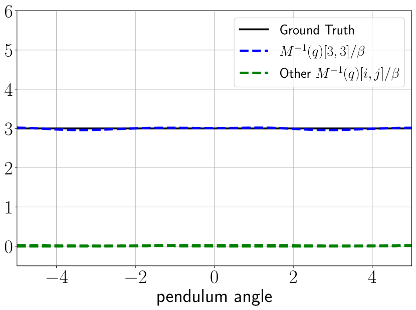
(a) $\mathbf{M}^{-1}(q)/\beta$ versus $\varphi$.

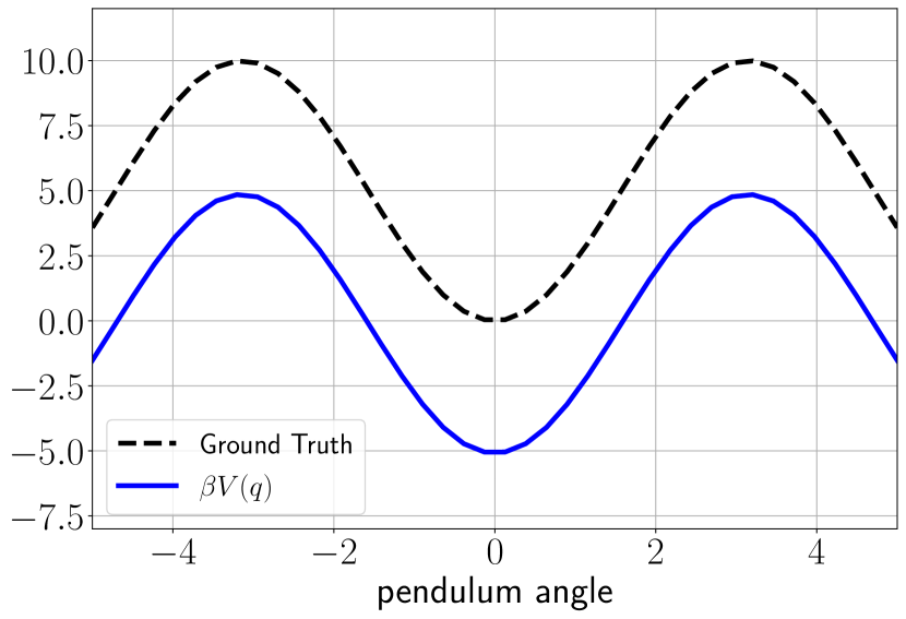
(b) $\beta{\cal V}({\boldsymbol{\mathfrak{q}}})$ versus $\varphi$.

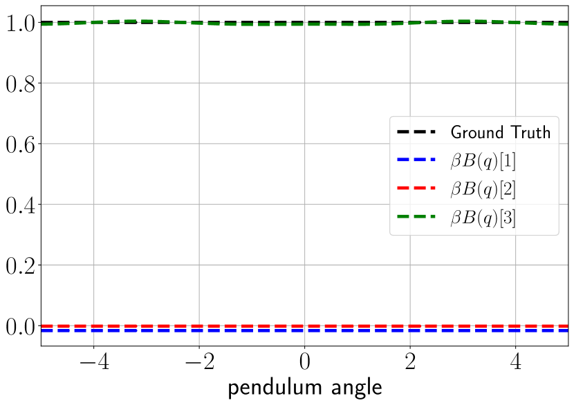
(c) $\beta\mathbf{B}({\boldsymbol{\mathfrak{q}}})$ versus $\varphi$.

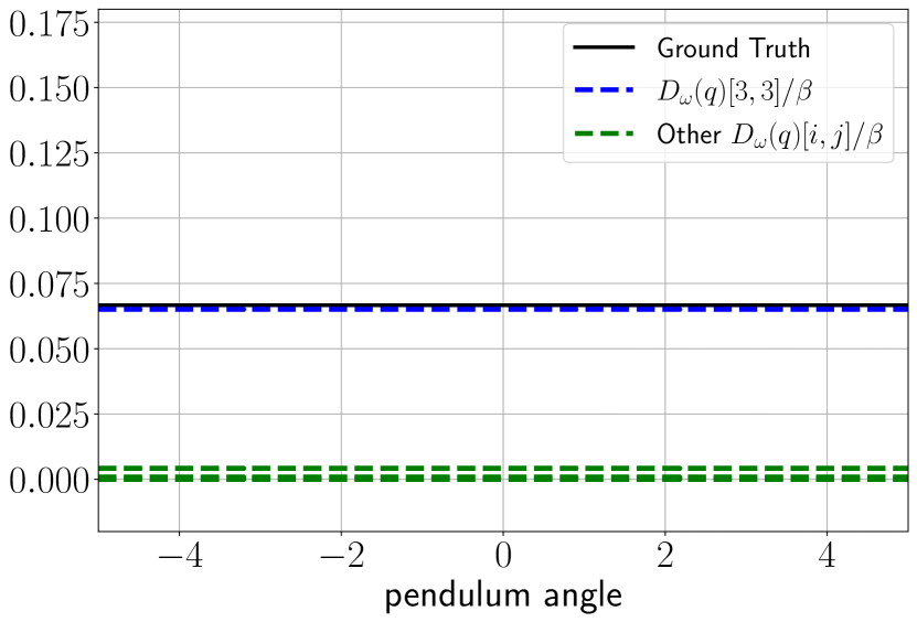
(d) $\mathbf{D}_{\omega}({\boldsymbol{\mathfrak{q}}})/\beta$ versus $\varphi$.

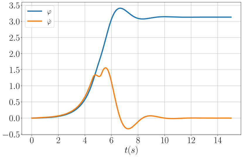
(e) Angle $\varphi$ and velocity $\dot{\varphi}$.

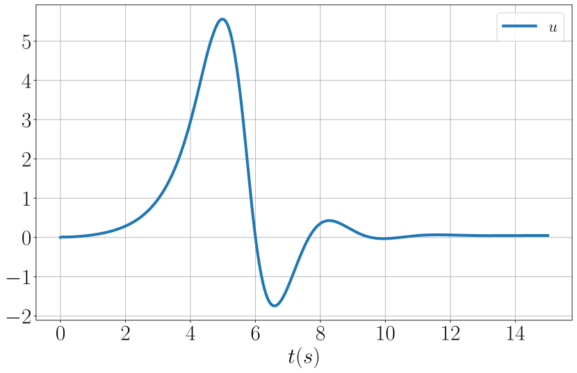
(f) Control input $u$.

Figure 3: Pendulum dynamics estimation using an $SO(3)$ port-Hamiltonian neural ODE network with scale factor $\beta=1.33$.

VII-A Pendulum

We consider a pendulum with the following dynamics:

$$\ddot{\varphi}=-15\sin{\varphi}+3u-0.2\dot{\varphi},$$ (68)

where $\varphi$ is the angle of the pendulum with respect to its vertically-downward position and $u$ is a scalar control input. The ground-truth mass, potential energy, friction coefficient, and the input gain are: $m=1/3$, ${\cal V}(\varphi)=5(1-\cos{\varphi})$, $D(\varphi)=0.2/3$, and $B(\varphi)=1$, respectively. We collected data of the form $\{(\cos{\varphi},\sin{\varphi},\dot{\varphi})\}$ from an OpenAI Gym environment, provided by [23], with the dynamics in (68). To illustrate our Lie group neural ODE learning, we represent the angle $\varphi$ as a rotation matrix:

$$\mathbf{R}=\begin{bmatrix}\cos{\varphi}&-\sin{\varphi}&0\\ \sin{\varphi}&\cos{\varphi}&0\\ 0&0&1\end{bmatrix},$$ (69)

representing the pendulum orientation. We let $\boldsymbol{\omega}=[0,0,\dot{\varphi}]$ and remove position $\mathbf{p}$ and linear velocity $\mathbf{v}$ from the Hamiltonian dynamics in (30), restricting the system to the $SO(3)$ manifold with generalized coordinates $\mathbf{{\boldsymbol{\mathfrak{q}}}}=[\mathbf{r}_{1}^{\top}\quad\mathbf{r}_{2}^{\top}\quad\mathbf{r}_{3}^{\top}]^{\top}$.

As described in Sec. V-D, control inputs $\mathbf{u}^{(i)}$ were sampled randomly and applied to the pendulum for five time intervals of $0.05s$, forming a dataset $\mathcal{D}=\left\{t_{0:N}^{(i)},\mathbf{{\boldsymbol{\mathfrak{q}}}}_{0:N}^{(i)},\boldsymbol{\omega}_{0:N}^{(i)},\mathbf{u}^{(i)})\right\}_{i=1}^{D}$ with $N=5$ and $D=5120$. We trained an $SO(3)$ port-Hamiltonian neural ODE network as described in Sec. V-D for $5000$ iterations without any nominal model, i.e., $\mathbf{M}^{-1}_{\boldsymbol{\omega}0}(\mathbf{{\boldsymbol{\mathfrak{q}}}})=\bf 0$, $\mathbf{D}_{\boldsymbol{\omega}0}({\boldsymbol{\mathfrak{q}}},{\boldsymbol{\mathfrak{p}}})=\bf 0$, $V_{0}({\boldsymbol{\mathfrak{q}}})=\bf 0$ and $\mathbf{B}_{0}({\boldsymbol{\mathfrak{q}}})=\bf 0$.

As noted in [23, 27], since the generalized momenta $\mathbf{{\boldsymbol{\mathfrak{p}}}}$ are not available in the dataset, the dynamics of $\mathbf{{\boldsymbol{\mathfrak{q}}}}$ in (68) do not change if $\mathbf{{\boldsymbol{\mathfrak{p}}}}$ is scaled by a factor $\beta>0$. This is also true in our formulation as scaling $\mathbf{{\boldsymbol{\mathfrak{p}}}}$ leaves the dynamics of $\mathbf{{\boldsymbol{\mathfrak{q}}}}$ in (30) unchanged. To emphasize this scale-invariance, let $\mathbf{M}_{\beta}(\mathbf{{\boldsymbol{\mathfrak{q}}}})=\beta\mathbf{M}(\mathbf{{\boldsymbol{\mathfrak{q}}}})$, ${\cal V}_{\beta}(\mathbf{{\boldsymbol{\mathfrak{q}}}})=\beta{\cal V}(\mathbf{{\boldsymbol{\mathfrak{q}}}})$, $\mathbf{D}_{\beta}(\mathbf{{\boldsymbol{\mathfrak{q}}}},\mathbf{{\boldsymbol{\mathfrak{p}}}})=\beta\mathbf{D}(\mathbf{{\boldsymbol{\mathfrak{q}}}},\mathbf{{\boldsymbol{\mathfrak{p}}}})$ $\mathbf{B}_{\beta}(\mathbf{{\boldsymbol{\mathfrak{q}}}})=\beta\mathbf{B}(\mathbf{{\boldsymbol{\mathfrak{q}}}})$, and:

$$\mathbf{{\boldsymbol{\mathfrak{p}}}}_{\beta} =\mathbf{M}_{\beta}(\mathbf{{\boldsymbol{\mathfrak{q}}}})\boldsymbol{\omega}=\beta\mathbf{{\boldsymbol{\mathfrak{p}}}},\quad\qquad\dot{\mathbf{{\boldsymbol{\mathfrak{p}}}}}_{\beta}=\beta\dot{\mathbf{{\boldsymbol{\mathfrak{p}}}}},$$ (70)

$$\mathcal{H}_{\beta}(\mathbf{{\boldsymbol{\mathfrak{q}}}},\mathbf{{\boldsymbol{\mathfrak{p}}}}) =\frac{1}{2}\mathbf{{\boldsymbol{\mathfrak{p}}}}_{\beta}^{\top}\mathbf{M}_{\beta}^{-1}(\mathbf{{\boldsymbol{\mathfrak{q}}}})\mathbf{{\boldsymbol{\mathfrak{p}}}}_{\beta}+V_{\beta}(\mathbf{{\boldsymbol{\mathfrak{q}}}})=\beta\mathcal{H}(\mathbf{{\boldsymbol{\mathfrak{q}}}},\mathbf{{\boldsymbol{\mathfrak{p}}}}),$$

$$\frac{\partial{\mathcal{H}_{\beta}(\mathbf{{\boldsymbol{\mathfrak{q}}}},\mathbf{{\boldsymbol{\mathfrak{p}}}})}}{\partial\mathbf{{\boldsymbol{\mathfrak{p}}}}_{\beta}} =\mathbf{M}^{-1}_{\beta}(\mathbf{{\boldsymbol{\mathfrak{q}}}})\mathbf{{\boldsymbol{\mathfrak{p}}}}_{\beta}=\frac{\partial{H(\mathbf{{\boldsymbol{\mathfrak{q}}}},\mathbf{{\boldsymbol{\mathfrak{p}}}})}}{\partial\mathbf{{\boldsymbol{\mathfrak{p}}}}},$$

guaranteeing that the equations of motions (30) still hold.

Fig. 3 shows the training and testing behavior of our $SO(3)$ Hamiltonian ODE network. Fig. 3(a) and 3(c) show that the $\left[\mathbf{M}(\mathbf{{\boldsymbol{\mathfrak{q}}}})^{-1}\right]_{3,3}$ entry of the mass inverse and the $\left[\mathbf{B}(\mathbf{{\boldsymbol{\mathfrak{q}}}})\right]_{3}$ entry of the input matrix with scaling factor $\beta=0.75$ are close to their correct values of $3$ and $1$, respectively, while the other entries are close to zero. Fig. 3(b) indicates a constant gap between the learned and the ground-truth potential energy, which can be explained by the relativity of potential energy.

We tested stabilization of the pendulum based on the learned dynamics to the unstable equilibrium at the upward position $\varphi=\pi$, with zero velocity. Since the pendulum is a fully-actuated system, the energy-based controller in (VI-B) exists and is obtained by removing the position error from the desired energy:

$$\mathcal{H}_{d}(\mathbf{{\boldsymbol{\mathfrak{q}}}}_{e},\mathbf{{\boldsymbol{\mathfrak{p}}}}_{e})=\frac{1}{2}\operatorname{tr}(\mathbf{K}_{\mathbf{R}}(\mathbf{I}-\mathbf{R}^{*\top}\mathbf{R}))+\frac{1}{2}{\boldsymbol{\mathfrak{p}}}_{\boldsymbol{\omega}}^{\top}\mathbf{M}^{-1}(\mathbf{{\boldsymbol{\mathfrak{q}}}}){\boldsymbol{\mathfrak{p}}}_{\boldsymbol{\omega}}.$$ (71)

The controlled angle $\varphi$ and angular velocity $\dot{\varphi}$ as well as the control inputs $\mathbf{u}$ with gains $\mathbf{K}_{\mathbf{R}}=2\mathbf{I}$ and $\mathbf{K}_{\mathbf{d}}=\mathbf{I}$ are shown over time in Fig. 3(e) and 3(f). We can see that the controller was able to smoothly drive the pendulum from $\phi=0$ to $\phi=\pi$, relying only on the learned dynamics.

VII-B Crazyflie Quadrotor

In this section, we demonstrate that our $SE(3)$ dynamics learning and control approach can achieve trajectory tracking for an underactuated system. We consider a Crazyflie quadrotor, shown in Fig. 6(a), simulated in the physics-based simulator PyBullet [72]. The control input $\mathbf{u}=[f,\boldsymbol{\tau}]$ includes a thrust $f\in\mathbb{R}_{\geq 0}$ and a torque vector $\boldsymbol{\tau}\in\mathbb{R}^{3}$ generated by the $4$ rotors. The generalized coordinates and velocity are $\mathbf{{\boldsymbol{\mathfrak{q}}}}=[\mathbf{p}^{\top}\quad\mathbf{r}_{1}^{\top}\quad\mathbf{r}_{2}^{\top}\quad\mathbf{r}_{3}^{\top}]^{\top}$ and $\boldsymbol{\zeta}=[\mathbf{v}^{\top}\quad\boldsymbol{\omega}^{\top}]^{\top}$ as before.

The quadrotor was controlled from a random starting point to $18$ different desired poses using a PID controller [72], providing $18$ $2.5$-second trajectories. The trajectories were used to generate a dataset $\mathcal{D}=\{t_{0:N}^{(i)},\mathbf{{\boldsymbol{\mathfrak{q}}}}_{0:N}^{(i)},\boldsymbol{\zeta}_{0:N}^{(i)},\mathbf{u}^{(i)})\}_{i=1}^{D}$ with $N=5$ and $D=1080$. The $SE(3)$ port-Hamiltonian ODE network was trained, as described in Sec. V-D, for $500$ iterations without a nominal model, i.e., $\mathbf{M}^{-1}_{\mathbf{v}0}(\mathbf{{\boldsymbol{\mathfrak{q}}}})=\bf 0$, $\mathbf{M}^{-1}_{\boldsymbol{\omega}0}(\mathbf{{\boldsymbol{\mathfrak{q}}}})=\bf 0$, $\mathbf{D}_{\mathbf{v}0}({\boldsymbol{\mathfrak{q}}},{\boldsymbol{\mathfrak{p}}})=\bf 0$, $\mathbf{D}_{\boldsymbol{\omega}0}({\boldsymbol{\mathfrak{q}}},{\boldsymbol{\mathfrak{p}}})=\bf 0$, $V_{0}({\boldsymbol{\mathfrak{q}}})=\bf 0$ and $\mathbf{B}_{0}({\boldsymbol{\mathfrak{q}}})=\bf 0$. We do not consider energy dissipation such as drag effect in the PyBullet simulator, and we omit the dissipation matrix $\mathbf{D}_{\boldsymbol{\theta}}({\boldsymbol{\mathfrak{q}}},{\boldsymbol{\mathfrak{p}}})$ in the model design.

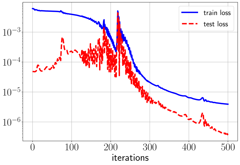
(a) Loss (log scale)

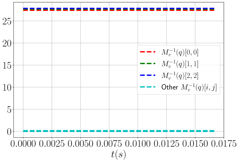
(b) $\mathbf{M}_{\mathbf{v}}^{-1}({\boldsymbol{\mathfrak{q}}})$

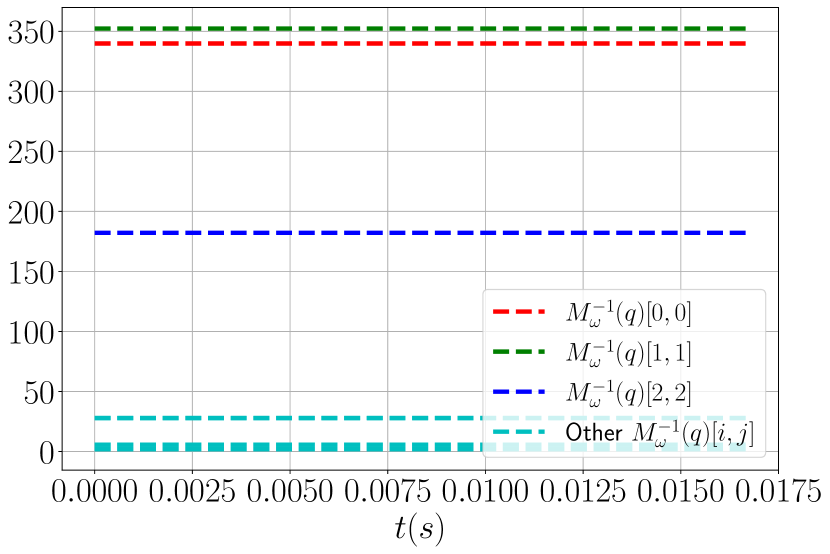
(c) $\mathbf{M}_{\boldsymbol{\omega}}^{-1}({\boldsymbol{\mathfrak{q}}})$

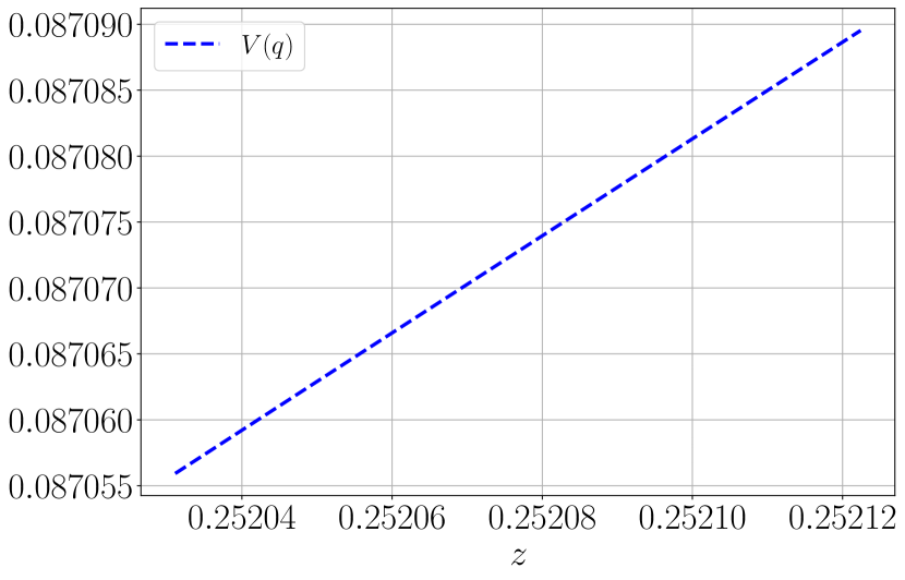
(d) ${\cal V}({\boldsymbol{\mathfrak{q}}})$

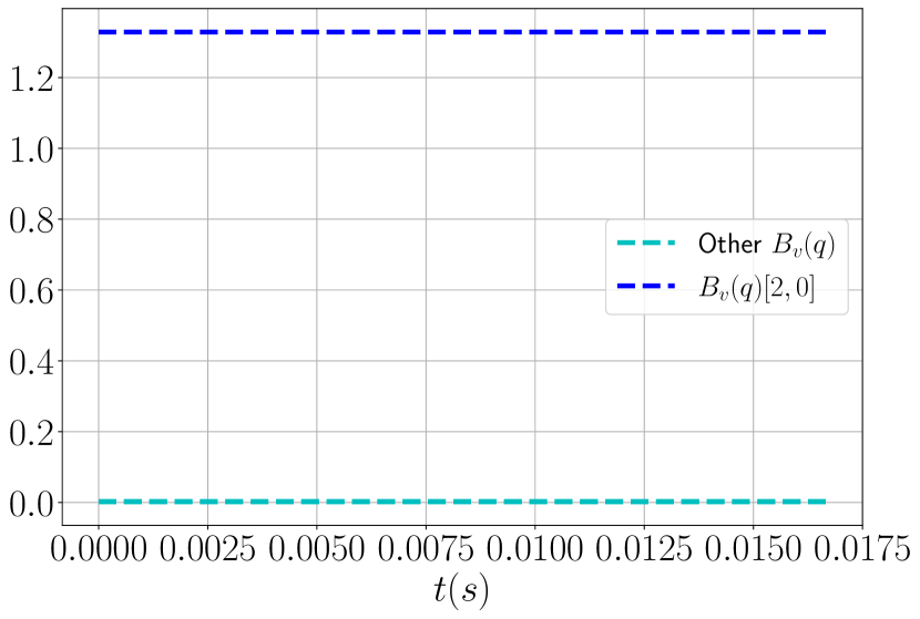
(e) $\mathbf{B}_{\mathbf{v}}({\boldsymbol{\mathfrak{q}}})$

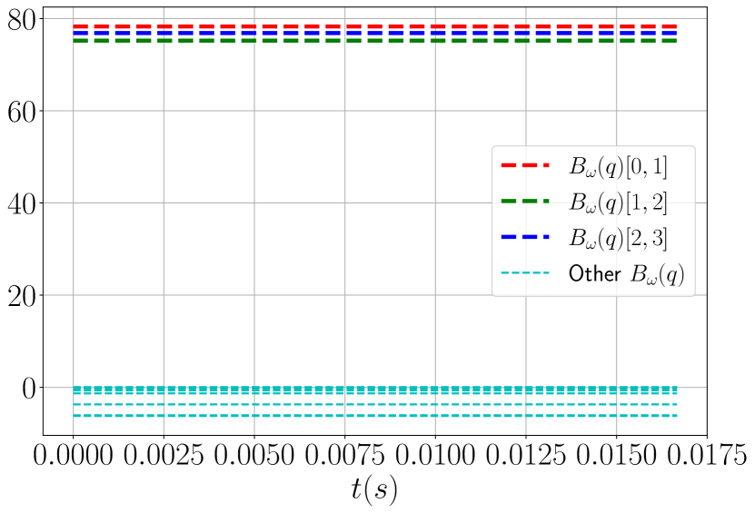
(f) $\mathbf{B}_{\boldsymbol{\omega}}({\boldsymbol{\mathfrak{q}}})$

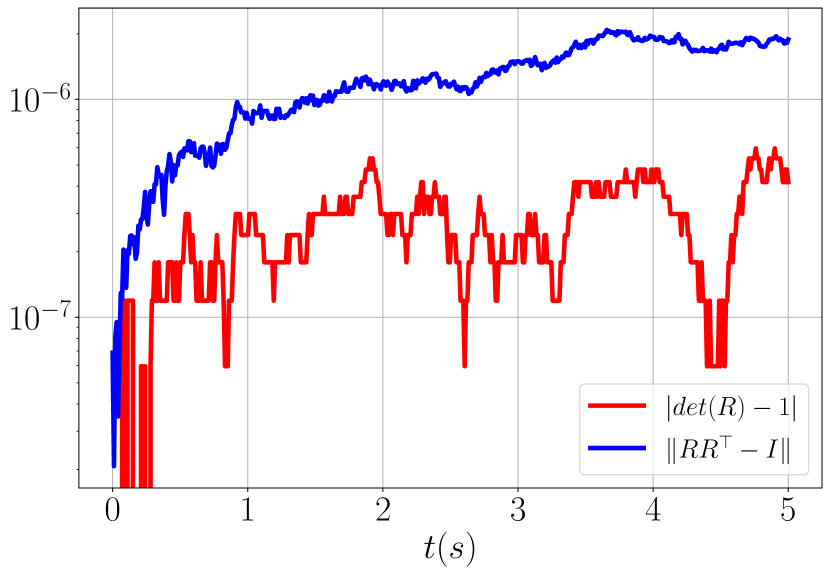
(g) SO(3) constraints.

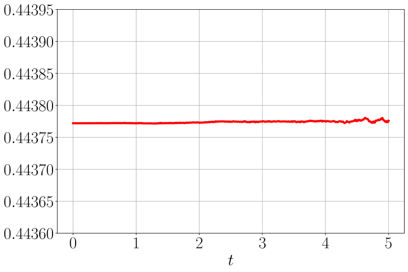
(h) Total energy.

Figure 4: Evaluation of $SE(3)$ port-Hamiltonian neural ODE network on a Crazyflie quadrotor in the PyBullet simulator [72].

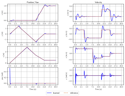
Figure 5: Crazyflie quadrotor trajectory (blue) tracking a desired diamond-shaped trajectory (orange) shown in Fig. 6.

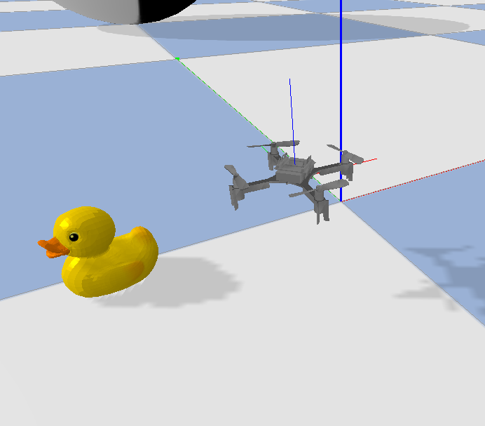
(a) Crazyflie simulator

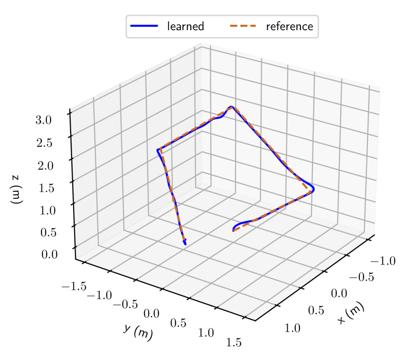
(b) Trajectory tracking

Figure 6: Trajectory tracking experiment with a Crazyflie quadrotor in the PyBullet simulator [72].

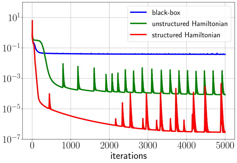
(a) Training loss

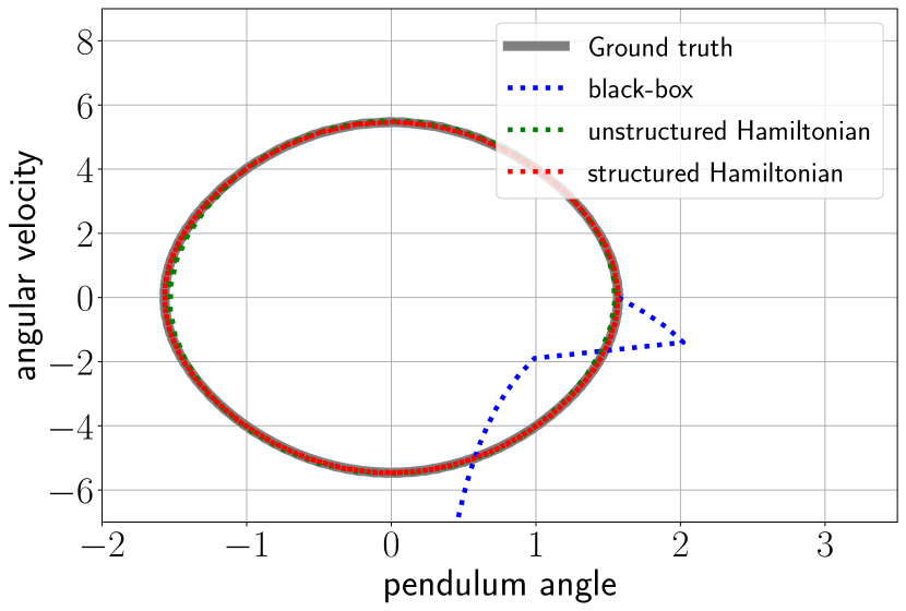
(b) Phase portraits

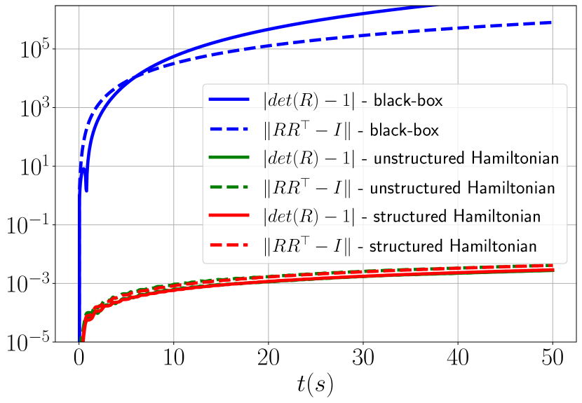
(c) SO(3) constraints

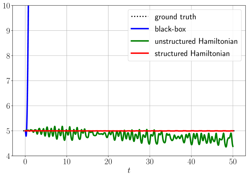
(d) Total energy

Figure 7: Comparison of different neural network architectures to learn pendulum dynamics: 1) black-box, i.e., the dynamics function $\mathbf{f}$ is represented by a multilayer perceptron network; 2) unstructured Hamiltonian, i.e., the Hamiltonian function is represented by a multilayer perceptron network instead of the sum of kinetic and potential energy as shown in Eq. (27); 3) structured Hamiltonian, i.e., the Hamiltonian function has the form of Eq. (27). Initialized at $\phi=\pi/2$, the learned pendulum dynamics are rolled out, showing that our approach with structured Hamiltonian preserves the phase portraits, $SO(3)$ constraints, and the conservation of energy better than the other models.

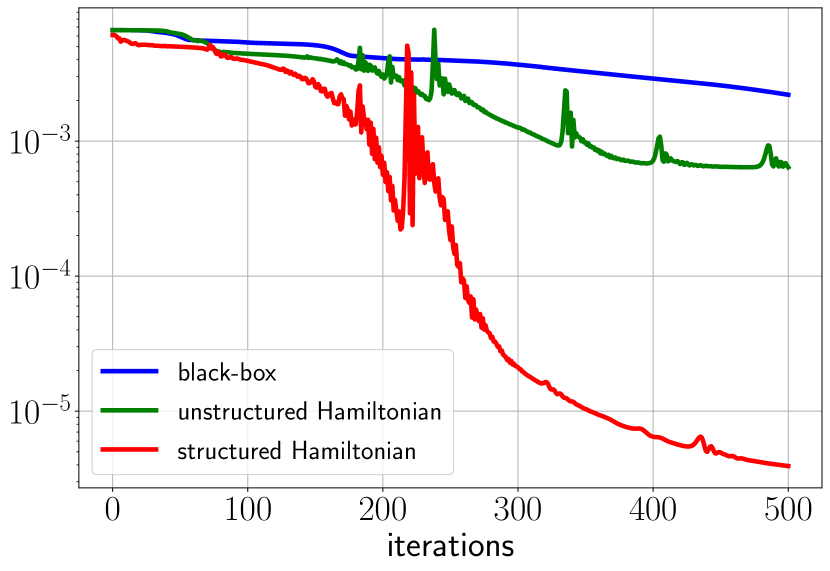
(a) Training loss

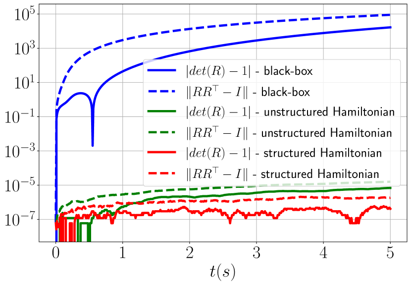
(b) SO(3) constraints

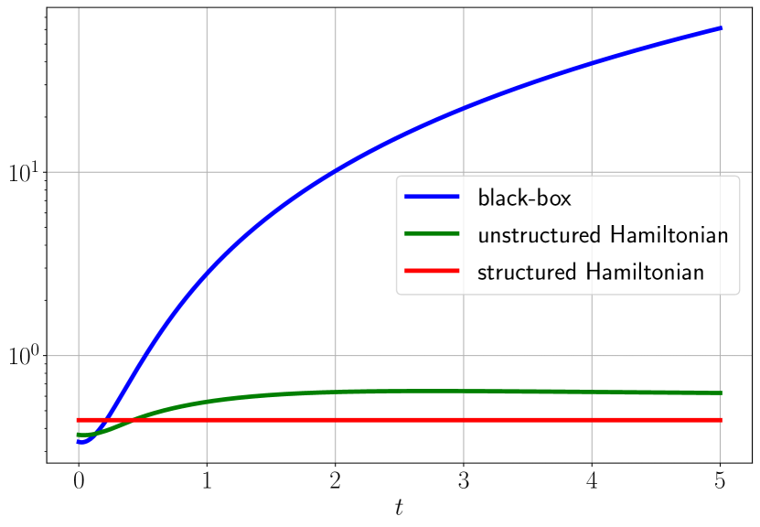
(c) Total energy

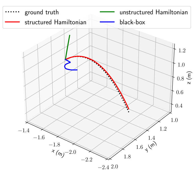
(d) Predicted trajectories

Figure 8: Comparison of different neural network architecture to learn quadrotor dynamics: 1) black-box, i.e., the dynamics function $\mathbf{f}$ is represented by a multilayer perceptron network; 2) unstructured Hamiltonian, i.e., the Hamiltonian function is represented by a multilayer perceptron network instead of the sum of kinetic and potential energy as shown in Eq. (27); 3) structured Hamiltonian, i.e., the Hamiltonian function has the form of Eq. (27). Initialized at a random pose and twist, the learned quadrotor dynamics are rolled out, showing that our approach with structured Hamiltonian preserves $SO(3)$ constraints and the conservation of energy better than the other models, and provides better state predictions.

The training and test results are shown in Fig. 4. The learned generalized mass and inertia converged to constant diagonal matrices: $\mathbf{M}_{\mathbf{v}}^{-1}(\mathbf{{\boldsymbol{\mathfrak{q}}}})\approx 27.5\mathbf{I}$, $\mathbf{M}_{\boldsymbol{\omega}}^{-1}(\mathbf{{\boldsymbol{\mathfrak{q}}}})\approx\text{diag}([351,340,181])$. The input matrix $\mathbf{B}_{\mathbf{v}}(\mathbf{{\boldsymbol{\mathfrak{q}}}})$ converged to a constant matrix with $\begin{bmatrix}\mathbf{B}_{\mathbf{v}}(\mathbf{{\boldsymbol{\mathfrak{q}}}})\end{bmatrix}_{2,0}\approx 1.32$ while the other entries were closed to $0$, consistent with the fact that the quadrotor thrust only affects the linear velocity along the $z$ axis in the body-fixed frame. The input matrix $\mathbf{B}_{\boldsymbol{\omega}}(\mathbf{{\boldsymbol{\mathfrak{q}}}})$ converged to $\sim 76\mathbf{I}$ as the motor torques affects all components of the angular velocity $\boldsymbol{\omega}$. The learned potential energy ${\cal V}(\mathbf{{\boldsymbol{\mathfrak{q}}}})$ was linear in the height $z$, agreeing with the gravitational potential.

We also verified our energy-based control design in Sec. VI by controlling the quadrotor to track a desired trajectory based on the learned dynamics model. Given desired position $\mathbf{p}^{*}$ and heading $\boldsymbol{\psi}^{*}$ (yaw angle), we construct an appropriate $\mathbf{R}^{*}$ and ${\boldsymbol{\mathfrak{p}}}^{*}$ to be used with the energy-based controller in (VI-B). By expanding the terms in (VI-B) and choosing the control gain $\mathbf{K}_{\mathbf{d}}$ of the form $\mathbf{K}_{\mathbf{d}}=\begin{bmatrix}\mathbf{K}_{v}&\bf 0\\ \bf 0&\mathbf{K}_{\omega}\end{bmatrix}$, the control input can be written explicitly as

$$\mathbf{u}=\mathbf{B}^{\dagger}(\mathbf{{\boldsymbol{\mathfrak{q}}}})\begin{bmatrix}\boldsymbol{\tau}_{\mathbf{v}}\\ \boldsymbol{\tau}_{\boldsymbol{\omega}}\end{bmatrix},$$ (72)

where

$$\boldsymbol{\tau}_{\mathbf{v}} = \mathbf{R}^{\top}\frac{\partial{\cal V}(\mathbf{{\boldsymbol{\mathfrak{q}}}})}{\partial\mathbf{p}}-\hat{\mathbf{{\boldsymbol{\mathfrak{p}}}}}_{\mathbf{v}}\boldsymbol{\omega}-\mathbf{R}^{\top}\mathbf{K}_{\mathbf{p}}(\mathbf{p}-\mathbf{p}^{*})$$ (73)

$$-\mathbf{K}_{\mathbf{v}}(\mathbf{v}-\mathbf{R}^{\top}\dot{\mathbf{p}}^{*})+\mathbf{M}_{1}(\mathbf{R}^{\top}\ddot{\mathbf{p}}^{*}-\hat{\boldsymbol{\omega}}\mathbf{R}^{\top}\dot{\mathbf{p}}^{*}),$$

$$\boldsymbol{\tau}_{\boldsymbol{\omega}} = \sum_{i=1}^{3}\hat{\mathbf{r}}_{i}\frac{\partial{\cal V}(\mathbf{{\boldsymbol{\mathfrak{q}}}})}{\partial\mathbf{r}_{i}}-\mathbf{K}_{\boldsymbol{\omega}}(\boldsymbol{\omega}-\mathbf{R}^{\top}\mathbf{R}^{*}\boldsymbol{\omega}^{*})$$ (74)

$$-(\hat{\mathbf{{\boldsymbol{\mathfrak{p}}}}}_{\boldsymbol{\omega}}\boldsymbol{\omega}+\hat{\mathbf{{\boldsymbol{\mathfrak{p}}}}}_{\mathbf{v}}\mathbf{v})-\frac{1}{2}\left(\mathbf{K}_{\mathbf{R}}\mathbf{R}^{*\top}\mathbf{R}-\mathbf{R}^{\top}\mathbf{R}^{*}\mathbf{K}_{\mathbf{R}}^{\top}\right)^{\vee}$$

$$+\mathbf{M}_{2}(\mathbf{R}^{\top}\mathbf{R}^{*}\dot{\boldsymbol{\omega}}^{*}-\hat{\boldsymbol{\omega}}_{e}\mathbf{R}^{\top}\mathbf{R}^{*}\boldsymbol{\omega}^{*}).$$

Note that $\boldsymbol{\tau}_{\mathbf{v}}\in\mathbb{R}^{3}$ is the desired thrust in the body frame and depends only on the desired position $\mathbf{p}^{*}$ and the current pose. The desired thrust is transformed to the world frame as $\mathbf{R}\boldsymbol{\tau}_{\mathbf{v}}$. Inspired by [70], the vector $\mathbf{R}\boldsymbol{\tau}_{\mathbf{v}}$ should be along the $z$ axis of the body frame, i.e., the third column $\mathbf{r}_{3}^{*}$ of the desired rotation matrix $\mathbf{R}^{*}$. The second column $\mathbf{r}^{*}_{2}$ of the desired rotation matrix $\mathbf{R}^{*}$ can be chosen so that it has the desired yaw angle $\psi^{*}$ and is perpendicular to $\mathbf{r}_{3}^{*}$. This can be done by projecting the second column of the yaw’s rotation matrix $\mathbf{r}_{2}^{\psi}=[-\sin{\psi},\cos{\psi},0]$ onto the plane perpendicular to $\mathbf{r}_{3}^{*}$. We have $\mathbf{R}^{*}=[\mathbf{r}_{1}^{*}\quad\mathbf{r}_{2}^{*}\quad\mathbf{r}_{3}^{*}]$ where:

$$\mathbf{r}_{3}^{*}=\frac{\mathbf{R}\boldsymbol{\tau}_{\mathbf{v}}}{\|\mathbf{R}\boldsymbol{\tau}_{\mathbf{v}}\|},\mathbf{r}_{1}^{*}=\frac{\mathbf{r}_{2}^{\psi}\times\mathbf{r}^{*}_{3}}{\|\mathbf{r}_{2}^{\psi}\times\mathbf{r}^{*}_{3}\|},\mathbf{r}_{2}^{*}=\mathbf{r}_{3}^{*}\times\mathbf{r}_{1}^{*},$$ (75)

and $\hat{\boldsymbol{\omega}}^{*}=\mathbf{R}^{*\top}\dot{\mathbf{R}}^{*}$. The derivative $\dot{\mathbf{R}}^{*}$ is calculated as follows:

$$\dot{\mathbf{r}}_{3}^{*} = \mathbf{r}_{3}^{*}\times\frac{\dot{\mathbf{R}\boldsymbol{\tau}_{\mathbf{v}}}}{\|\mathbf{R}\boldsymbol{\tau}_{\mathbf{v}}\|}\times\mathbf{r}_{3}^{*},$$ (76)

$$\dot{\mathbf{r}}_{1}^{*} = \mathbf{r}_{1}^{*}\times\frac{\dot{\mathbf{r}}_{2}^{\psi}\times\mathbf{r}_{3}^{*}+\mathbf{r}_{2}^{\psi}\times\dot{\mathbf{r}}_{3}^{*}}{\|\mathbf{r}_{2}^{\psi}\times\mathbf{r}_{3}^{*}\|}\times\mathbf{r}_{1}^{*},$$ (77)

$$\dot{\mathbf{r}}_{2}^{*} = \dot{\mathbf{r}}_{3}^{*}\times\mathbf{r}_{1}^{*}+\mathbf{r}_{3}^{*}\times\dot{\mathbf{r}}_{1}^{*}.$$ (78)

Plugging $\mathbf{R}^{*}$ and $\boldsymbol{\omega}^{*}$ back in $\boldsymbol{\tau}_{\boldsymbol{\omega}}$, we obtain the complete control input $\mathbf{u}$ in (72).

Fig. 6(b) shows qualitatively that the quadrotor controlled by our energy-based controller achieves successful trajectory tracking. The control gains were chosen as: $\mathbf{K}_{\mathbf{p}}=\operatorname{diag}([0.8,0.8,3.9])$, $\mathbf{K}_{\mathbf{v}}=0.23\mathbf{I},\mathbf{K}_{\mathbf{R}}=\operatorname{diag}([3.6,3.6,6.9])$, $\mathbf{K}_{\boldsymbol{\omega}}=\operatorname{diag}([0.3,0.3,0.6])$. Fig. 4 shows quantitatively the tracking errors in the position, yaw angles, linear velocity, and angular velocity. On an Intel i9 3.1 GHz CPU with 32GB RAM, our controller’s computation time in Python 3.7 was about $2.5$ ms per control input, including forward passes through the neural networks, showing that it is suitable for fast real-time applications.

VII-C Comparison to Unstructured Neural ODE Models

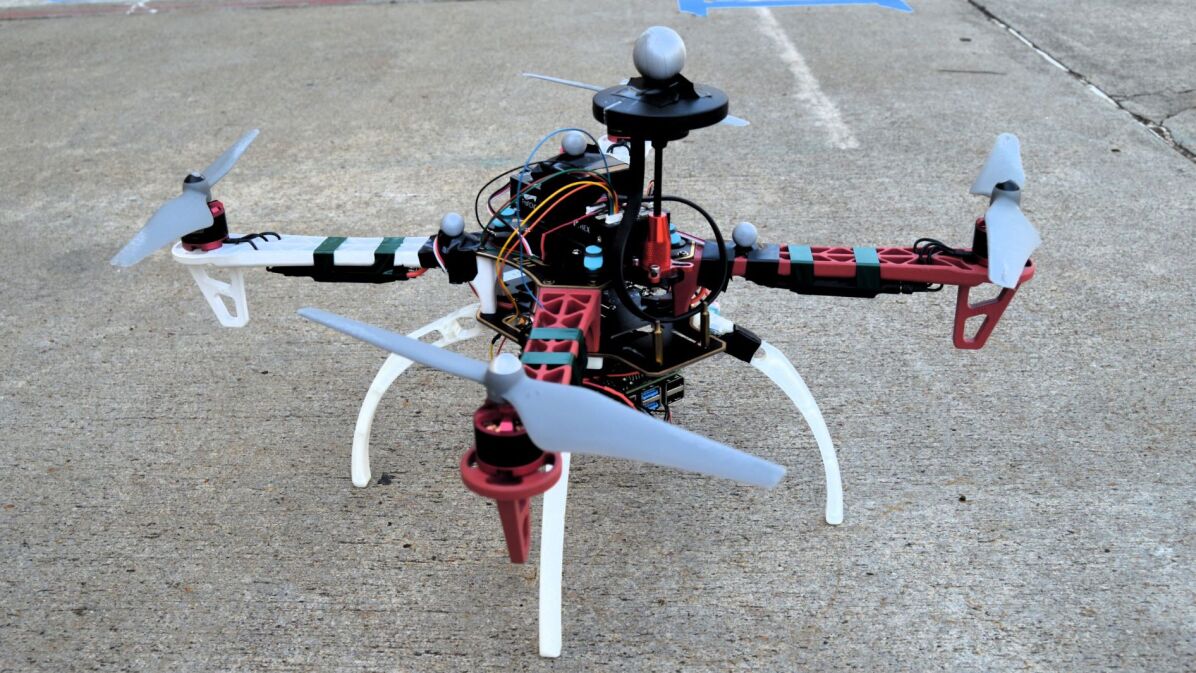
(a) RaspberryPi drone

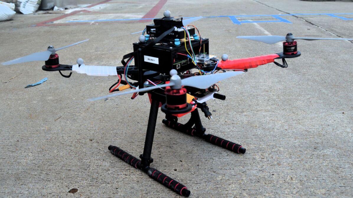
(b) Intel NUC drone

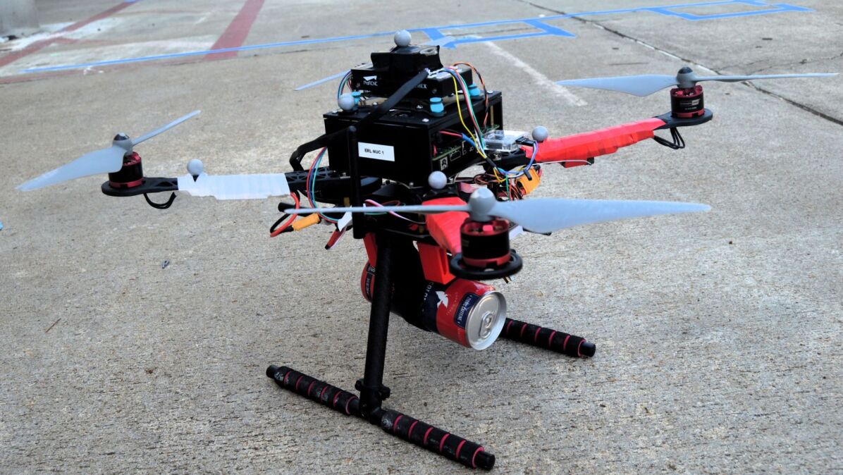
(c) Intel NUC drone with payload

Figure 9: Quadrotor robots used in the experiments: (a) RaspberryPi quadrotor whose mass and inertia matrix serve as nominal values for our learning framework, (b) Intel NUC quadrotor with a different frame, and (c) Intel NUC quadrotor carrying a coffee can as payload.

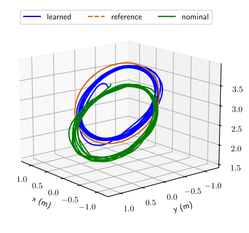
(a) Vertical circle

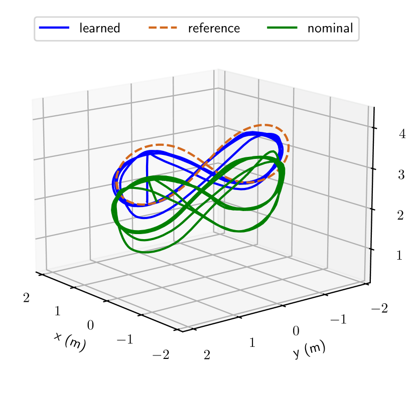
(b) Vertical lemniscate

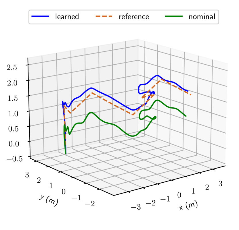
(c) Piecewise linear

Figure 10: Trajectory tracking with real quadrotors: (a) vertical circle, (b) vertical lemniscate, (c) piecewise linear trajectory.

In this section, we show the benefits of our neural ODE architecture by comparing 1) our structured Hamiltonian model, 2) a black-box model, i.e., the approximated dynamics $\mathbf{f}$ is represented by a multilayer perceptron network, and 3) an unstructured Hamiltonian model, i.e., the Hamiltonian function is represented by a multilayer perceptron network instead of using the structure in Eq. (27), in terms of training convergence rates, guarantees of energy conservation principle, and Lie group constraint satisfaction. To verify energy conservation, we rolled out the learned dynamics and calculated the Hamiltonian via (27) along the predicted trajectories for (1) the black-box model using ground-truth mass and potential energy with the predicted states; (2) the unstructured Hamiltonian model using the output of the multilayer perceptron Hamiltonian network; and (3) the structured Hamiltonian model using the learned mass and potential energy networks. We check the $SO(3)$ constraints by verifying that two quantities $|\det{\mathbf{R}}-1|$ and $\|\mathbf{R}\mathbf{R}^{\top}-\mathbf{I}\|$ remain small along the predicted trajectories.

We first use a pendulum as described in Sec. VII-A without energy dissipation. The models are trained for $5000$ iterations from $512$ 0.2-second state-control trajectories and rolled out for a significantly longer horizon of $50$ seconds. Fig. 7 plots the training loss, the phase portraits, the SO(3) constraints and the total energy (Hamiltonian) of the learned models for a pendulum system. As the Hamiltonian structure is imposed in the neural ODE network architecture, our model is able to converge faster with lower loss (Fig. 7(a)) and preserves the phase portraits for state predictions (Fig. 7(b)). Fig. 7(c) shows that the $SO(3)$ constraints are satisfied by our structured and unstructured Hamiltonian models as their values of $|\det{\mathbf{R}}-1|$ and $\|\mathbf{R}\mathbf{R}^{\top}-\mathbf{I}\|$ remain small along a $50$-second trajectory rollout initialized at $\phi=\pi/2$. The constant Hamiltonian in Fig. 7(d) of our structured Hamiltonian verifies that our model obeys the energy conservation law with no control input and no energy dissipation. The Hamiltonian of the black-box model increases along the trajectory while that of the unstructured Hamiltonian model fluctuates and slightly decreases over time.

We also tested the models using the simulated Crazyflie quadtoror with the same dataset ${\cal D}$ of $18$ trajectories as described in Sec. VII-B. The $SE(3)$ port-Hamiltonian ODE network was trained, as described in Sec. V-D, for $500$ iterations. Our structured Hamiltonian model converges faster with significantly lower loss as seen in Fig. 8(a). We verified that the predicted orientation trajectories from our learned models satisfy the $SO(3)$ constraints. Fig. 8(b) shows two near-zero quantities $|\det{\mathbf{R}}-1|$ and $\|\mathbf{R}\mathbf{R}^{\top}-\mathbf{I}\|$, obtained by rolling out our learned dynamics for $5$ seconds, while the learned black-box model violates the constraints after a very short time. Fig. 8(c) shows a constant total energy along the predicted trajectory from our structured Hamiltonian model without control input and dissipation networks, verifying that the learned model obeys the law of energy conservation. Fig. 8(d) shows that our structured Hamiltonian model provides better trajectory predictions compared to the other methods.

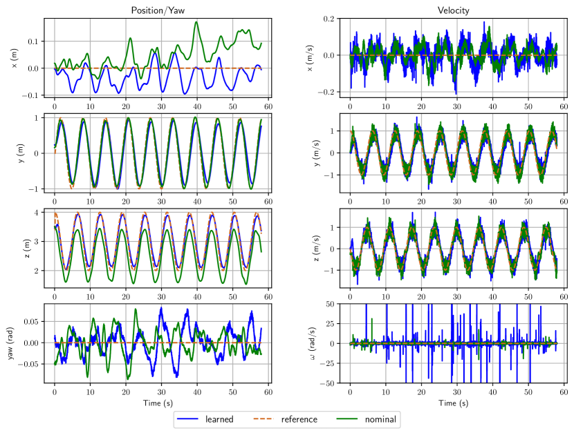
(a) Vertical circle

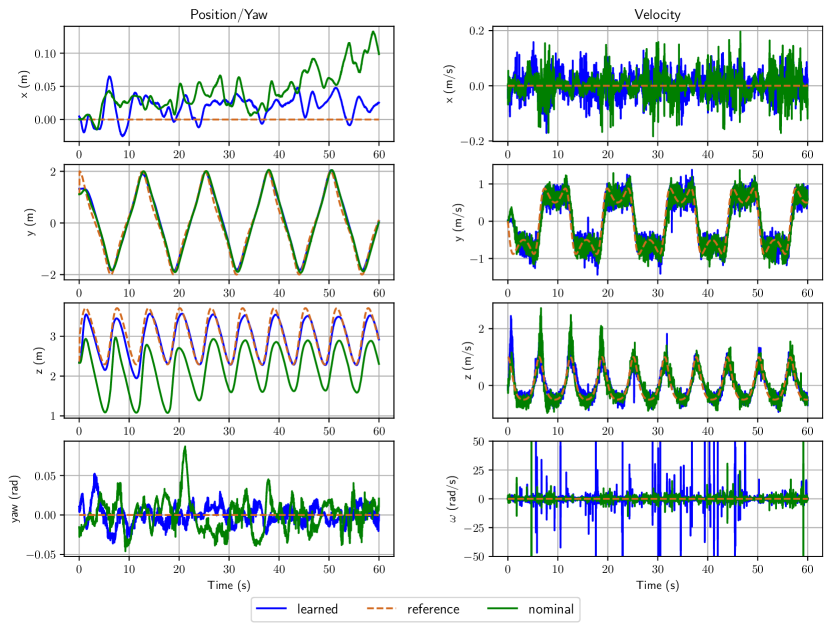
(b) Vertical lemniscate

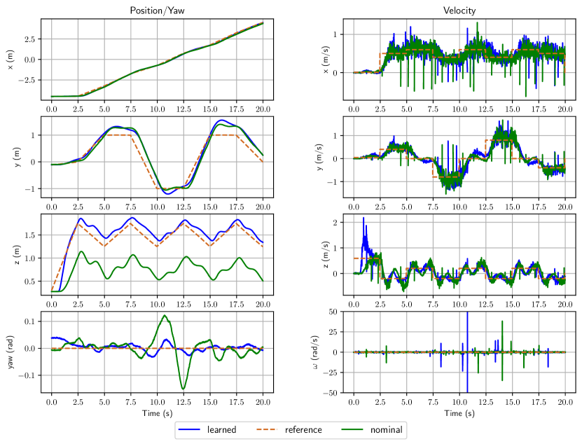
(c) Piecewise-linear

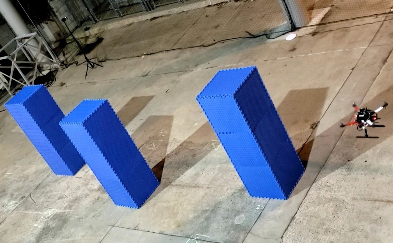
(d) Tracking at $t=0$s

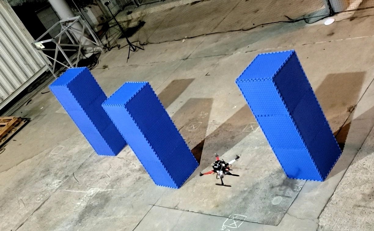
(e) Tracking at $t=3$s

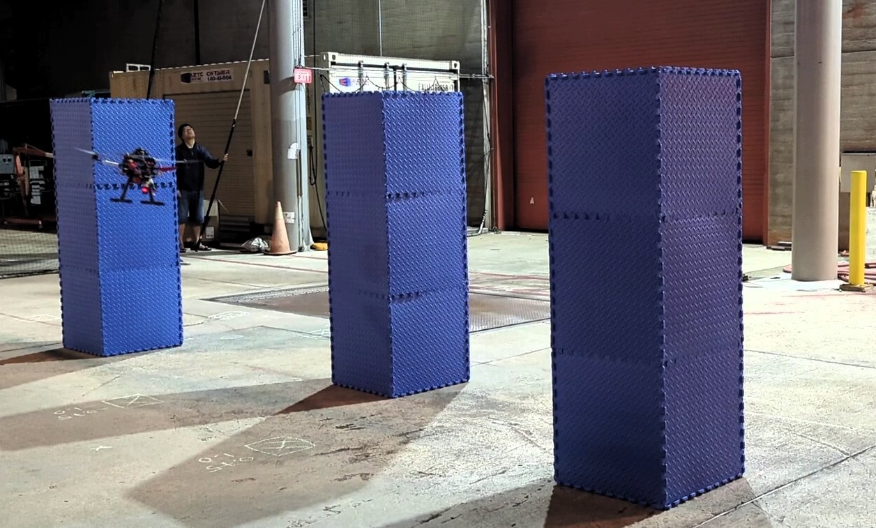
(f) Tracking at $t=9$s

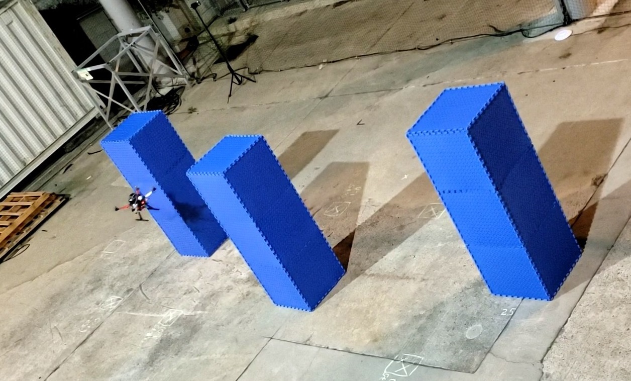
(g) Tracking at $t=12$s

Figure 11: Real quadrotor trajectory using our learned model and controller (blue) and using a nominal model and a geometric controller [70] (green) tracking a desired trajectory.

VII-D Real Quadrotor Experiments

In this section, we verify our approach using a real quadrotor robot, equipped with an onboard i7 Intel NUC computer and a PX4 flight controller (see Fig. 9(b)). The quadrotor’s pose and twist were provided by a motion capture system.

VII-D1 Learning quadrotor dynamics after upgrade

We consider a scenario in which the quadrotor is upgraded with a new frame and a new onboard computer, leading to changes in the robot dynamics that we aim to learn from data. The mass and inertia matrix of a previous model (Fig. 9(a)) with Raspberry Pi computer and an F450 frame were used as the nominal mass $\mathbf{M}_{\mathbf{v}0}=1.3\mathbf{I}$ and inertia matrix $\mathbf{M}_{\boldsymbol{\omega}0}=\operatorname{diag}([0.12,0.12,0.2])$ for the upgraded quadrotor (Fig. 9(b)). The other nominal matrices were set to zero: $\mathbf{D}_{\mathbf{v}0}({\boldsymbol{\mathfrak{q}}},{\boldsymbol{\mathfrak{p}}})=\bf 0$, $\mathbf{D}_{\boldsymbol{\omega}0}({\boldsymbol{\mathfrak{q}}},{\boldsymbol{\mathfrak{p}}})=\bf 0$, $V_{0}({\boldsymbol{\mathfrak{q}}})=\bf 0$ and $\mathbf{B}_{0}({\boldsymbol{\mathfrak{q}}})=\bf 0$. We modified the PX4 firmware [73] to expose the normalized thrust and torque being sent to the motors. The firmware’s normalization of thrust and torque is unknown and, in fact, is learned from data via the input gain matrix $\mathbf{B}({\boldsymbol{\mathfrak{q}}})$. We collected $12$ state-control trajectories by flying the quadrotor from a starting pose to $12$ different poses using a PID controller provided by the PX4 flight controller [73]. The trajectories were used to generate a dataset $\mathcal{D}=\{t_{0:N}^{(i)},\mathbf{{\boldsymbol{\mathfrak{q}}}}_{0:N}^{(i)},\boldsymbol{\zeta}_{0:N}^{(i)},\mathbf{u}^{(i)})\}_{i=1}^{D}$ with $N=1$ and $D=~{}10000$. We trained our model as described in Sec. V-D for $5000$ steps.

The trained model was used with the control policy in Sec. VII-B to track different trajectories: a verticle circle, a vertical lemniscate, and a 3D piecewise-linear trajectories. Fig. 10 and 11 show that we achieve better tracking performance using our learned dynamics model and energy-based control compared to the nominal model and the geometric controller in [70]. The tracking errors of our controller with a learned model improve by $2-4$ times compared to those of geometric control based on the nominal model, as shown in Table I.

TABLE I: Position tracking errors using nominal and learned quadrotor models with and without payload.

Model Train Test Circle Lemniscate Piecewise- with with linear payload payload Nominal - No $0.26~{}(m)$ $0.52~{}(m)$ $0.62~{}(m)$ Learned No No $\mathbf{0.13(m)}$ $\mathbf{0.14(m)}$ $\mathbf{0.22(m)}$ Learned No Yes $0.20~{}(m)$ $0.40~{}(m)$ $0.30~{}(m)$ Learned Yes Yes $\mathbf{0.13~{}(m)}$ $\mathbf{0.12~{}(m)}$ $\mathbf{0.21~{}(m)}$

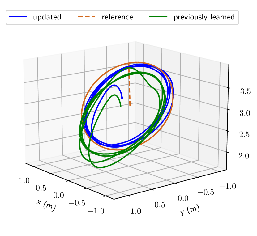
(a) Vertical circle

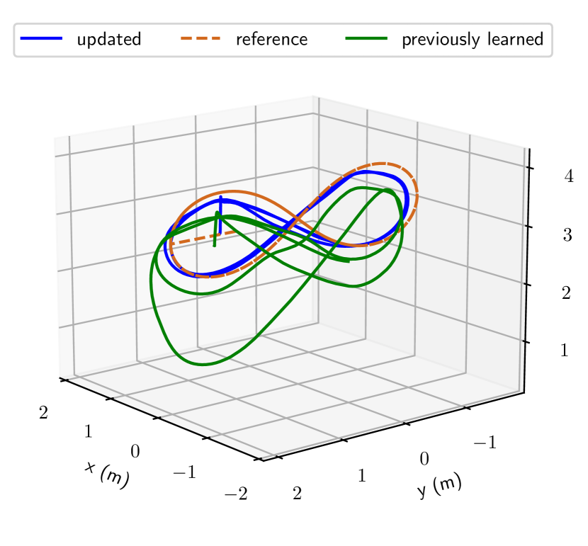
(b) Vertical lemniscate

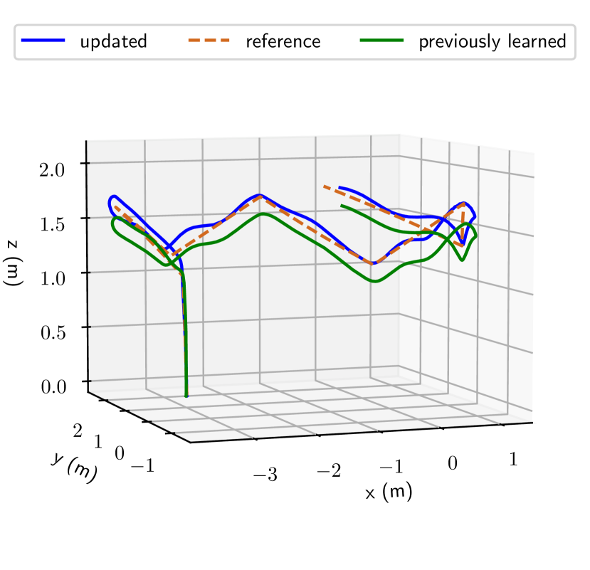
(c) Piecewise linear

Figure 12: Quadrotor trajectory tracking experiment with extra payload: vertical circle (a), vertical lemniscate (b), piecewise linear trajectory (c).

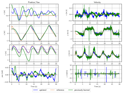
Figure 13: Tracking a piecewise-linear trajectory with extra payload using our previously learned and updated models.

VII-D2 Learning quadrotor dynamics with extra payload

In this section, we demonstrate that after our dynamics model is trained, if there is a change in the quadrotor dynamics, e.g., an extra payload is added, we are able to update the dynamics quickly starting from the previously trained model. We attached a coffee can to the quadrotor frame (Fig. 9(c)) to change the mass and inertia matrix of the robot. We, then, collected a new dataset by driving the quadrotor to $12$ different poses, and trained our dynamics model for only $100$ steps, initialized with the trained model in Sec. VII-D1.

In the presence of the coffee can payload, the tracking performance of the controller with the previously learned model degrades as shown in Fig. 12 and 13. Meanwhile, after a quick model update, the robot is able to track desired trajectories accurately again. Table I shows that our updated model improves the tracking errors by $1.5$–$4$ times compared to the previously learned model.

VIII Conclusion

This paper proposed a neural ODE network design for robot dynamics learning that captures Lie group kinematics, e.g. $SE(3)$, and port-Hamiltonian dynamics constraints by construction. It also developed a general control approach for trajectory tracking based on the learned Lie group port-Hamiltonian dynamics. The learning and control designs are not system-specific and, thus, can be applied to different types of robots whose states evolve on Lie group. These techniques have the potential to enable robots to quickly adapt their models online, in response to changing operational conditions or structural damage, and continue to maintain stability during autonomous operation. Future work will focus on extending our formulation to allow learning multi-rigid-body dynamics, handling contact, and online adaptation to disturbances and structural changes in the dynamics.

IX Appendix

IX-A Implementation Details

We used fully-connected neural networks whose architecture is shown below. The first number is the input dimension while the last number is the output dimension. The numbers in between are the hidden layers’ dimensions and activation functions. The value of $\varepsilon_{\mathbf{v}}$ and $\varepsilon_{\boldsymbol{\omega}}$ in (40) is set to $0.01$.

1. Pendulum:

   • Input dimension: $9$. Action dimension: $1$.

   • $\mathbf{L}(\mathbf{{\boldsymbol{\mathfrak{q}}}})$:
     9 - 300 Tanh - 300 Tanh - 300 Tanh - 300 Linear - 6.

   • ${\cal V}_{\boldsymbol{\theta}}(\mathbf{{\boldsymbol{\mathfrak{q}}}})$: 9 - 50 Tanh - 50 Tanh - 50 Linear - 1.

   • $\mathbf{B}_{\boldsymbol{\theta}}(\mathbf{{\boldsymbol{\mathfrak{q}}}})$: 9 - 300 Tanh - 300 Tanh - 300 Linear - 3.

2. Pybullet quadrotor:

   • Input dimension: $12$. Action dimension: $4$.

   • $\mathbf{L}_{\mathbf{v}}(\mathbf{{\boldsymbol{\mathfrak{q}}}})$ only takes the position $\mathbf{p}\in\mathbb{R}^{3}$ as input:
     3 - 400 Tanh - 400 Tanh - 400 Tanh - 400 Linear - 6.

   • $\mathbf{L}_{\boldsymbol{\omega}}(\mathbf{{\boldsymbol{\mathfrak{q}}}})$ only takes the rotation matrix $\mathbf{R}\in\mathbb{R}^{3\times 3}$ as input:
     9 - 400 Tanh - 400 Tanh - 400 Tanh - 400 Linear - 6.

   • ${\cal V}_{\boldsymbol{\theta}}(\mathbf{{\boldsymbol{\mathfrak{q}}}})$: 12 - 400 Tanh - 400 Tanh - 400 Linear - 1.

   • $\mathbf{B}_{\boldsymbol{\theta}}(\mathbf{{\boldsymbol{\mathfrak{q}}}})$: 12 - 400 Tanh - 400 Tanh - 400 Linear - 24.

3. Real PX4 quadrotor:

   • Input dimension: $12$. Action dimension: $4$.

   • $\mathbf{L}_{\mathbf{v}}(\mathbf{{\boldsymbol{\mathfrak{q}}}})$ only takes the position $\mathbf{p}\in\mathbb{R}^{3}$ as input:
     3 - 20 Tanh - 20 Tanh - 20 Tanh - 20 Linear - 6.

   • $\mathbf{L}_{\boldsymbol{\omega}}(\mathbf{{\boldsymbol{\mathfrak{q}}}})$ only takes the rotation matrix $\mathbf{R}\in\mathbb{R}^{3\times 3}$ as input:
     9 - 20 Tanh - 20 Tanh - 20 Tanh - 20 Linear - 6.

   • $\mathbf{D}_{\mathbf{v};{\boldsymbol{\theta}}}(\mathbf{{\boldsymbol{\mathfrak{q}}}})$ only takes the position $\mathbf{p}\in\mathbb{R}^{3}$ as input:
     3 - 20 Tanh - 20 Tanh - 20 Tanh - 20 Linear - 6.

   • $\mathbf{D}_{\boldsymbol{\omega};{\boldsymbol{\theta}}}(\mathbf{{\boldsymbol{\mathfrak{q}}}})$ only takes the rotation matrix $\mathbf{R}\in\mathbb{R}^{3\times 3}$ as input:
     9 - 20 Tanh - 20 Tanh - 20 Tanh - 20 Linear - 6.

   • $V(\mathbf{{\boldsymbol{\mathfrak{q}}}})$: 12 - 20 Tanh - 20 Tanh - 20 Linear - 1.

   • $\mathbf{B}_{\boldsymbol{\theta}}(\mathbf{{\boldsymbol{\mathfrak{q}}}})$: 12 - 20 Tanh - 20 Tanh - 20 Linear - 24.

Thai Duong is a PhD candidate in Electrical and Computer Engineering at the University of California, San Diego. He received a B.S. degree in Electronics and Telecommunications from Hanoi University of Science and Technology, Hanoi, Vietnam in 2011 and an M.S. degree in Electrical and Computer Engineering from Oregon State University, Corvallis, OR, in 2013. His research interests include machine learning with applications to robotics, mapping and active exploration using mobile robots, robot dynamics learning, planning and control.

Abdullah Altawaitan is a Ph.D. student in Electrical and Computer Engineering at the University of California San Diego, La Jolla, CA, USA. He received both the B.S. and M.S. degrees in Electrical Engineering from Arizona State University, Tempe, AZ, USA. He is also affiliated with the Electrical Engineering Department, College of Engineering and Petroleum, Kuwait University, Safat, Kuwait. His research interests include machine learning, control theory, and their applications to robotics.

Jason Stanley is an undergraduate student in the Electrical and Computer Engineering department at the University of California, San Diego (UCSD). He is pursuing a major in Computer Engineering, and is planning to continue and do a Masters in Electrical Engineering, also at UCSD. His research interests include control theory, machine learning for robotics, and mobile robots.

Nikolay Atanasov (S’07-M’16-SM’23) is an Assistant Professor of Electrical and Computer Engineering at the University of California San Diego, La Jolla, CA, USA. He obtained a B.S. degree in Electrical Engineering from Trinity College, Hartford, CT, USA in 2008 and M.S. and Ph.D. degrees in Electrical and Systems Engineering from the University of Pennsylvania, Philadelphia, PA, USA in 2012 and 2015, respectively. Dr. Atanasov’s research focuses on robotics, control theory, and machine learning, applied to active perception problems for autonomous mobile robots. He works on probabilistic models that unify geometric and semantic information in simultaneous localization and mapping (SLAM) and on optimal control and reinforcement learning algorithms for minimizing probabilistic model uncertainty. Dr. Atanasov’s work has been recognized by the Joseph and Rosaline Wolf award for the best Ph.D. dissertation in Electrical and Systems Engineering at the University of Pennsylvania in 2015, the Best Conference Paper Award at the IEEE International Conference on Robotics and Automation (ICRA) in 2017, the NSF CAREER Award in 2021, and the IEEE RAS Early Academic Career Award in Robotics and Automation in 2023.

References

• [1] L. Ljung, “System identification,” Wiley encyclopedia of electrical and electronics engineering, 1999.
• [2] D. Nguyen-Tuong and J. Peters, “Model learning for robot control: a survey,” Cognitive processing, vol. 12, no. 4, 2011.
• [3] M. Deisenroth and C. E. Rasmussen, “PILCO: A model-based and data-efficient approach to policy search,” in International Conference on Machine Learning (ICML), 2011.
• [4] G. Williams, N. Wagener, B. Goldfain, P. Drews, J. M. Rehg, B. Boots, and E. A. Theodorou, “Information theoretic MPC for model-based reinforcement learning,” in IEEE International Conference on Robotics and Automation (ICRA), 2017.
• [5] M. Raissi, P. Perdikaris, and G. E. Karniadakis, “Multistep neural networks for data-driven discovery of nonlinear dynamical systems,” arXiv preprint arXiv:1801.01236, 2018.
• [6] K. Chua, R. Calandra, R. McAllister, and S. Levine, “Deep reinforcement learning in a handful of trials using probabilistic dynamics models,” in Advances in Neural Information Processing Systems (NeurIPS), 2018.
• [7] M. Lutter and J. Peters, “Combining physics and deep learning to learn continuous-time dynamics models,” The International Journal of Robotics Research, vol. 42, no. 3, pp. 83–107, 2023. [Online]. Available: https://doi.org/10.1177/02783649231169492
• [8] J. K. Gupta, K. Menda, Z. Manchester, and M. J. Kochenderfer, “A general framework for structured learning of mechanical systems,” arXiv preprint arXiv:1902.08705, 2019.
• [9] M. Cranmer, S. Greydanus, S. Hoyer, P. Battaglia, D. Spergel, and S. Ho, “Lagrangian neural networks,” in ICLR 2020 Workshop on Integration of Deep Neural Models and Differential Equations, 2020.
• [10] S. Greydanus, M. Dzamba, and J. Yosinski, “Hamiltonian neural networks,” in Advances in Neural Information Processing Systems (NeurIPS), vol. 32, 2019.
• [11] Z. Chen, J. Zhang, M. Arjovsky, and L. Bottou, “Symplectic recurrent neural networks,” International Conference on Learning Representations (ICLR), 2020.
• [12] M. A. Roehrl, T. A. Runkler, V. Brandtstetter, M. Tokic, and S. Obermayer, “Modeling system dynamics with physics-informed neural networks based on Lagrangian mechanics,” arXiv preprint arXiv:2005.14617, 2020.
• [13] Y. Lu, S. Lin, G. Chen, and J. Pan, “ModLaNets: Learning generalisable dynamics via modularity and physical inductive bias,” in Proceedings of the 39th International Conference on Machine Learning, ser. Proceedings of Machine Learning Research, K. Chaudhuri, S. Jegelka, L. Song, C. Szepesvari, G. Niu, and S. Sabato, Eds., vol. 162.   PMLR, 2022.
• [14] C. Neary and U. Topcu, “Compositional learning of dynamical system models using port-hamiltonian neural networks,” in Learning for Dynamics and Control Conference.   PMLR, 2023, pp. 679–691.
• [15] A. Sanchez-Gonzalez, N. Heess, J. T. Springenberg, J. Merel, M. Riedmiller, R. Hadsell, and P. Battaglia, “Graph networks as learnable physics engines for inference and control,” in International Conference on Machine Learning (ICML), 2018.
• [16] M. Lutter, C. Ritter, and J. Peters, “Deep Lagrangian networks: using physics as model prior for deep learning,” in International Conference on Learning Representations (ICLR), 2018.
• [17] B. C. Hall, Lie groups, Lie algebras, and representations.   Springer, 2013.
• [18] K. M. Lynch and F. C. Park, Modern Robotics: Mechanics, Planning, and Control.   Cambridge University Press, 2017.
• [19] A. I. Lurie, Analytical mechanics.   Springer Science & Business Media, 2013.
• [20] D. D. Holm, Geometric Mechanics.   World Scientific Publishing Company, 2008.
• [21] T. Bertalan, F. Dietrich, I. Mezić, and I. G. Kevrekidis, “On learning Hamiltonian systems from data,” Chaos: An Interdisciplinary Journal of Nonlinear Science, vol. 29, no. 12, 2019.
• [22] M. Finzi, K. A. Wang, and A. G. Wilson, “Simplifying Hamiltonian and Lagrangian neural networks via explicit constraints,” in Advances in Neural Information Processing Systems (NeurIPS), vol. 33, 2020.
• [23] Y. D. Zhong, B. Dey, and A. Chakraborty, “Symplectic ODE-Net: learning Hamiltonian dynamics with control,” in International Conference on Learning Representations (ICLR), 2019.
• [24] J. Willard, X. Jia, S. Xu, M. Steinbach, and V. Kumar, “Integrating physics-based modeling with machine learning: A survey,” arXiv preprint arXiv:2003.04919, 2020.
• [25] A. J. Maciejewski, “Hamiltonian formalism for euler parameters,” Celestial Mechanics, vol. 37, no. 1, 1985.
• [26] R. Shivarama and E. P. Fahrenthold, “Hamilton’s equations with Euler parameters for rigid body dynamics modeling,” Journal of Dynamic Systems, Measurement, and Control, vol. 126, no. 1, 2004.
• [27] T. Duong and N. Atanasov, “Hamiltonian-based Neural ODE Networks on the SE(3) Manifold For Dynamics Learning and Control,” in Proceedings of Robotics: Science and Systems, Virtual, July 2021.
• [28] R. T. Chen, Y. Rubanova, J. Bettencourt, and D. Duvenaud, “Neural ordinary differential equations,” in Advances in Neural Information Processing Systems (NeurIPS), 2018.
• [29] T. Lee, M. Leok, and N. H. McClamroch, Global formulations of Lagrangian and Hamiltonian dynamics on manifolds.   Springer, 2017.
• [30] Y. D. Zhong, B. Dey, and A. Chakraborty, “Dissipative SymODEN: Encoding Hamiltonian dynamics with dissipation and control into deep learning,” in ICLR 2020 Workshop on Integration of Deep Neural Models and Differential Equations, 2020.
• [31] A. Van Der Schaft and D. Jeltsema, “Port-Hamiltonian systems theory: An introductory overview,” Foundations and Trends in Systems and Control, vol. 1, no. 2-3, 2014.
• [32] Y. Song, A. Romero, M. Müller, V. Koltun, and D. Scaramuzza, “Reaching the limit in autonomous racing: Optimal control versus reinforcement learning,” Science Robotics, vol. 8, no. 82, p. eadg1462, 2023. [Online]. Available: https://www.science.org/doi/abs/10.1126/scirobotics.adg1462
• [33] T. Salzmann, E. Kaufmann, J. Arrizabalaga, M. Pavone, D. Scaramuzza, and M. Ryll, “Real-time neural mpc: Deep learning model predictive control for quadrotors and agile robotic platforms,” IEEE Robotics and Automation Letters, vol. 8, no. 4, pp. 2397–2404, 2023.
• [34] D. Scaramuzza and E. Kaufmann, “Learning agile, vision-based drone flight: From simulation to reality,” in The International Symposium of Robotics Research.   Springer, 2022, pp. 11–18.
• [35] A. Loquercio, E. Kaufmann, R. Ranftl, M. Müller, V. Koltun, and D. Scaramuzza, “Learning high-speed flight in the wild,” Science Robotics, vol. 6, no. 59, p. eabg5810, 2021.
• [36] J. Ibarz, J. Tan, C. Finn, M. Kalakrishnan, P. Pastor, and S. Levine, “How to train your robot with deep reinforcement learning: lessons we have learned,” The International Journal of Robotics Research, vol. 40, no. 4-5, pp. 698–721, 2021.
• [37] T. X. Nghiem, J. Drgoňa, C. Jones, Z. Nagy, R. Schwan, B. Dey, A. Chakrabarty, S. Di Cairano, J. A. Paulson, A. Carron et al., “Physics-informed machine learning for modeling and control of dynamical systems,” arXiv preprint arXiv:2306.13867, 2023.
• [38] F. Djeumou, C. Neary, E. Goubault, S. Putot, and U. Topcu, “Neural networks with physics-informed architectures and constraints for dynamical systems modeling,” in Learning for Dynamics and Control Conference.   PMLR, 2022, pp. 263–277.
• [39] A. J. Thorpe, C. Neary, F. Djeumou, M. M. Oishi, and U. Topcu, “Physics-informed kernel embeddings: Integrating prior system knowledge with data-driven control,” arXiv preprint arXiv:2301.03565, 2023.
• [40] L. Ruthotto and E. Haber, “Deep neural networks motivated by partial differential equations,” Journal of Mathematical Imaging and Vision, 2019.
• [41] R. Wang, R. Walters, and R. Yu, “Incorporating symmetry into deep dynamics models for improved generalization,” in International Conference on Learning Representations (ICLR), 2021.
• [42] M. Lutter, K. Listmann, and J. Peters, “Deep Lagrangian Networks for end-to-end learning of energy-based control for under-actuated systems,” in IEEE/RSJ International Conference on Intelligent Robots and Systems (IROS), 2019.
• [43] T. Beckers, J. Seidman, P. Perdikaris, and G. J. Pappas, “Gaussian process port-hamiltonian systems: Bayesian learning with physics prior,” in 2022 IEEE 61st Conference on Decision and Control (CDC).   IEEE, 2022, pp. 1447–1453.
• [44] T. Beckers, “Data-driven Bayesian Control of Port-Hamiltonian Systems,” in IEEE Conference on Decision and Control (CDC), 2023.
• [45] B. Leimkuhler and S. Reich, Simulating Hamiltonian dynamics.   Cambridge University Press, 2004.
• [46] P. Toth, D. J. Rezende, A. Jaegle, S. Racanière, A. Botev, and I. Higgins, “Hamiltonian generative networks,” in International Conference on Learning Representations (ICLR), 2019.
• [47] J. Mason, C. Allen-Blanchette, N. Zolman, E. Davison, and N. Leonard, “Learning interpretable dynamics from images of a freely rotating 3d rigid body,” arXiv preprint arXiv:2209.11355, 2022.
• [48] J. E. Marsden and M. West, “Discrete mechanics and variational integrators,” Acta Numer., vol. 10, pp. 357–514, 2001.
• [49] A. Havens and G. Chowdhary, “Forced variational integrator networks for prediction and control of mechanical systems,” in Learning for Dynamics and Control (L4DC), 2021, pp. 1142–1153.
• [50] V. Duruisseaux, T. Duong, M. Leok, and N. Atanasov, “Lie Group Forced Variational Integrator Networks for Learning and Control of Robot Systems,” in Learning for Dynamics and Control (L4DC), 2023, pp. 731–744.
• [51] R. Chen and M. Tao, “Data-driven prediction of general hamiltonian dynamics via learning exactly-symplectic maps,” in Proceedings of the 38th International Conference on Machine Learning, ser. Proceedings of Machine Learning Research, M. Meila and T. Zhang, Eds., vol. 139.   PMLR, 2021, pp. 1717–1727.
• [52] O. So, G. Li, E. A. Theodorou, and M. Tao, “Data-driven discovery of non-newtonian astronomy via learning non-euclidean hamiltonian,” ICML Machine Learning and the Physical Sciences Workshop, 2022.
• [53] F. Borrelli, A. Bemporad, and M. Morari, Predictive control for linear and hybrid systems.   Cambridge University Press, 2017.
• [54] R. Ortega, M. W. Spong, F. Gómez-Estern, and G. Blankenstein, “Stabilization of a class of underactuated mechanical systems via interconnection and damping assignment,” IEEE Transactions on Automatic Control, vol. 47, no. 8, 2002.
• [55] J. Á. Acosta, M. Sanchez, and A. Ollero, “Robust control of underactuated aerial manipulators via IDA-PBC,” in IEEE Conference on Decision and Control (CDC).   IEEE, 2014.
• [56] O. B. Cieza and J. Reger, “IDA-PBC for underactuated mechanical systems in implicit Port-Hamiltonian representation,” in European Control Conference (ECC), 2019.
• [57] Z. Wang and P. Goldsmith, “Modified energy-balancing-based control for the tracking problem,” IET Control Theory & Applications, vol. 2, no. 4, 2008.
• [58] C. Souza, G. V. Raffo, and E. B. Castelan, “Passivity based control of a quadrotor UAV,” IFAC Proceedings Volumes, vol. 47, no. 3, 2014.
• [59] L. Furieri, C. L. Galimberti, M. Zakwan, and G. Ferrari-Trecate, “Distributed neural network control with dependability guarantees: a compositional port-hamiltonian approach,” in Learning for Dynamics and Control Conference.   PMLR, 2022, pp. 571–583.
• [60] C. L. Galimberti, L. Furieri, L. Xu, and G. Ferrari-Trecate, “Hamiltonian deep neural networks guaranteeing nonvanishing gradients by design,” IEEE Transactions on Automatic Control, vol. 68, no. 5, pp. 3155–3162, 2023.
• [61] E. Sebastián, T. Duong, N. Atanasov, E. Montijano, and C. Sagüés, “LEMURS: Learning distributed multi-robot interactions,” in IEEE International Conference on Robotics and Automation (ICRA), 2023, pp. 7713–7719.
• [62] J. E. Marsden and T. S. Ratiu, Introduction to mechanics and symmetry: a basic exposition of classical mechanical systems.   Springer Science & Business Media, 2013, vol. 17.
• [63] T. D. Barfoot, State Estimation for Robotics.   Cambridge University Press, 2017.
• [64] M. Faessler, A. Franchi, and D. Scaramuzza, “Differential flatness of quadrotor dynamics subject to rotor drag for accurate tracking of high-speed trajectories,” IEEE Robotics and Automation Letters, vol. 3, no. 2, 2017.
• [65] P. Forni, D. Jeltsema, and G. A. Lopes, “Port-Hamiltonian formulation of rigid-body attitude control,” IFAC-PapersOnLine, vol. 48, no. 13, 2015.
• [66] R. Rashad, F. Califano, and S. Stramigioli, “Port-Hamiltonian passivity-based control on SE(3) of a fully actuated UAV for aerial physical interaction near-hovering,” IEEE Robotics and Automation Letters, vol. 4, no. 4, 2019.
• [67] J. Delmerico and D. Scaramuzza, “A benchmark comparison of monocular visual-inertial odometry algorithms for flying robots,” in IEEE International Conference on Robotics and Automation (ICRA), 2018.
• [68] S. A. S. Mohamed, M. Haghbayan, T. Westerlund, J. Heikkonen, H. Tenhunen, and J. Plosila, “A survey on odometry for autonomous navigation systems,” IEEE Access, vol. 7, 2019.
• [69] A. Paszke, S. Gross, F. Massa, A. Lerer, J. Bradbury, G. Chanan, T. Killeen, Z. Lin, N. Gimelshein, L. Antiga, A. Desmaison, A. Kopf, E. Yang, Z. DeVito, M. Raison, A. Tejani, S. Chilamkurthy, B. Steiner, L. Fang, J. Bai, and S. Chintala, “PyTorch: An Imperative Style, High-Performance Deep Learning Library,” in Advances in Neural Information Processing Systems 32, 2019, pp. 8024–8035.
• [70] T. Lee, M. Leok, and N. H. McClamroch, “Geometric tracking control of a quadrotor UAV on SE(3),” in IEEE Conference on Decision and Control (CDC), 2010.
• [71] H. K. Khalil, Nonlinear systems.   Prentice hall, 2002.
• [72] J. Panerati, H. Zheng, S. Zhou, J. Xu, A. Prorok, and A. P. Schöllig, “Learning to fly: a pybullet gym environment to learn the control of multiple nano-quadcopters,” https://github.com/utiasDSL/gym-pybullet-drones, 2020.
• [73] L. Meier, D. Honegger, and M. Pollefeys, “Px4: A node-based multithreaded open source robotics framework for deeply embedded platforms,” in IEEE International Conference on Robotics and Automation (ICRA), 2015, pp. 6235–6240.