Exact Analytical Solution of the One-Dimensional Time-Dependent Radiative Transfer Equation with Linear Scattering

Abstract

The radiative transfer equation (RTE) is a cornerstone for describing the propagation of electromagnetic radiation in a medium, with applications spanning atmospheric science, astrophysics, remote sensing, and biomedical optics. Despite its importance, an exact analytical solution to the RTE has remained elusive, necessitating the use of numerical approximations such as Monte Carlo, discrete ordinate, and spherical harmonics methods.

In this paper, we present an exact solution to the one-dimensional time-dependent RTE. We delve into the moments of the photon distribution, providing a clear view of the transition to the diffusion regime. This analysis offers a deeper understanding of light propagation in the medium.

Furthermore, we demonstrate that the one-dimensional RTE is equivalent to the Klein-Gordon equation with an imaginary mass term determined by the inverse reduced scattering length. Contrary to naive expectations of superluminal solutions, we find that our solution is strictly causal under appropriate boundary conditions, determined by the light transport problem.

We validate the found solution using Monte Carlo simulations and benchmark the performance of the latter. Our analysis reveals that even for highly forward scattering, dozens of random light scatterings are required for an accurate estimate, underscoring the complexity of the problem.

Moreover, we propose a method for faster convergence by adjusting the parameters of Monte Carlo sampling. We show that a Monte Carlo method sampling photon scatterings with input parameters $(\mu_{s},g)$, where $\mu_{s}$ is the inverse scattering length and $g$ is the scattering anisotropy parameter, is equivalent to that with $(\mu_{s}(1-g)/2,-1)$. This equivalence leads to a significantly faster convergence to the exact solution, offering a substantial improvement of the Monte Carlo method for the one-dimensional RTE.

Our findings not only contribute to the theoretical understanding of the RTE but also have potential implications for improving the numerical methods used to approximate it.

I Introduction

The study of light propagation in random media is critical to many fields in fundamental and applied science. The Radiative Transfer Equation (RTE), a classical integro-differential equation, is a useful approximation for describing light propagation in these media. While the one-dimensional RTE is applied to various physical systems, such as atmospheric science [1, 2], astrophysics [3], remote sensing [4], and biomedical optics [5], an exact analytic solution is not available for even simple cases. Although a solution exists for the steady-state one-dimensional RTE [6], there is no known solution for the time-dependent one-dimensional RTE.

The main goal of this study is to derive an analytic solution to the time-dependent one-dimensional RTE for the propagation of light in random media, such as water or ice. Our objective is to use this solution and its generalization to the three-dimensional case to simulate the response of neutrino telescopes [7, 8, 9, 10].

This article presents the exact solution to the one-dimensional RTE. The paper is structured as follows. Section II formulates the one-dimensional RTE and its solution. In section III, we discuss the results. In particular, in section III.1 the moments of the photon’s distribution are discussed which allows to explicitly observe a change to the diffusion regime. In section III.2 we observe that one-dimensional RTE is equivalent to the Klein-Gordon equation with the imaginary mass term determined by the inverse reduced scattering length. However, in a stark contrast to naive expectations of superluminal solution, the solution which we find is strictly casual under appropriate boundary conditions. In section III.3 we benchmark a Monte Carlo method and its convergence to the exact solution. We find that an accurate description requires an accounting for dozens of light scatterings. In section III.4 we also propose a method for faster convergence by changing the parameters of Monte Carlo sampling. Finally, in section III.5 we provide a general discussion of the Monte Carlo convergence rate to the true solution.

The technical details of the derivation of the solution and its validation are presented in Appendix A. In Appendix B, we demonstrate that a new Monte Carlo sampling method is equivalent to the original method for an infinite number of scatterings, while converging to the exact solution faster.

Finally, Section IV concludes our study.

II Solution to one-dimensional RTE

Let us denote by $L(l,x,s)$ the absolute value of a flux of photons (units: $\text{m}^{-2}$) at position $x$, time $t$ and direction $s=\pm 1$, corresponding to photon movement to the right ($s=+1$) or to the left ($s=-1$) along $x$. This function obeys the following time-dependent radiative transfer equation, drastically simplified for one-dimension,

$$\left(\partial_{l}+s\partial_{x}+\mu_{t}\right)L(l,x,s)=\mu_{s}\sum_{s^{\prime}=\pm 1}P(s,s^{\prime})L(l,x,s^{\prime}),$$ (1)

where $\partial_{x}=\partial/\partial x$, $\partial_{l}=\partial/\partial l$ with $l=ct$ being the total path length travelled with speed $c$ during time $t$ along the axis $x$, $c$ is the speed of light in the medium, $\mu_{t}$ is a sum of absorption $\mu_{a}$ and scattering $\mu_{s}$ inverse wavelengths. The probability density scattering function $P(s,s^{\prime})$ takes one of two possible values

$$P(+1,+1) =P(-1,-1)=\frac{1+g}{2},$$ (2)

$$P(+1,-1) =P(-1,+1)=\frac{1-g}{2},$$

with the sum of these quantities equal to one. The parameter $g$ can be interpreted as scattering asymmetry: $g=1$ corresponds to the forward scattering, $g=-1$ to the backward scattering, and $g=0$ to equal chances of scattering back and forth.

Introducing

$$L_{\pm}(l,x)=e^{\mu_{t}l}L(l,x,\pm 1),$$ (3)

eq. 1 could be re-written as a system of coupled equations

$$\partial_{l}L_{+}+\partial_{x}L_{+}=\mu_{s}\left(\frac{1+g}{2}L_{+}+\frac{1-g}{2}L_{-}\right),$$ (4)

$$\partial_{l}L_{-}-\partial_{x}L_{-}=\mu_{s}\left(\frac{1-g}{2}L_{+}+\frac{1+g}{2}L_{-}\right).$$

As one could observe, eq. 1 does not contain the source function. Instead, we shall consider the initial conditions

$$L(0,x,+1) =L_{+}(0,x)=\delta(x),$$ (5)

$$L(0,x,-1) =L_{-}(0,x)=0,$$

which correspond to a photon at the origin $x=0$ moving to the right at $t=0$.

Substitutions

$$L_{+} =e^{\mu_{s}(1+g)l/2}\widetilde{L}_{+},$$ (6)

$$L_{-} =e^{\mu_{s}(1+g)l/2}\widetilde{L}_{-}$$

lead to the following system of equations relating $\widetilde{L}_{\pm}$

$$(\partial_{l}+\partial_{x})\widetilde{L}_{+} =\lambda\widetilde{L}_{-},$$ (7)

$$(\partial_{l}-\partial_{x})\widetilde{L}_{-} =\lambda\widetilde{L}_{+},$$

where

$$\lambda=\mu^{\prime}_{s}/2,\quad\mu_{s}^{\prime}=\mu_{s}(1-g).$$ (8)

The solution to eq. 7 with initial conditions in eq. 5 is found to be

$$\widetilde{L}_{+}(l,x) =\delta(l-x)+\frac{\lambda}{2}\widetilde{\theta}(\tau^{2})\sqrt{\frac{l+x}{l-x}}I_{1}(\lambda\tau),$$ (9)

$$\widetilde{L}_{-}(l,x) =\frac{\lambda}{2}\widetilde{\theta}(\tau^{2})I_{0}(\lambda\tau),$$

with

$$\widetilde{\theta}(\tau^{2})=(1-\theta(-\tau^{2})),\tau=\sqrt{l^{2}-x^{2}},$$ (10)

where $\theta(z)$ and $\widetilde{\theta}(z)$ are two Heaviside functions with a distinct definition at the zero argument

$$\theta(z)=\begin{cases}1,&z\geq 0\\ 0,&z<0\end{cases},\text{ and }\widetilde{\theta}(z)=\begin{cases}1,&z>0\\ 0,&z\leq 0\end{cases}.$$ (11)

The solution to eq. 9 is casual and valid for both domains $l\geq 0$ and $l<0$. Multiplication of $\widetilde{L}_{\pm}$ by $\theta(l)$ ($\theta(-l)$), also proven to be the solution to eq. 7, corresponds to the retarded (advanced) casual Green functions. A derivation of this solution can be found in appendix A.

Functions $I_{n}(z)$ in eq. 9 refer to the modified Bessel functions of the first kind. $I_{n}(z)$ are exponentially growing functions for $z\to\infty$. However, the solution to eq. 1 is finite everywhere because of the additional exponential factor in eq. 6

$$L(l,x,+1)=e^{-(\mu_{a}+\mu^{\prime}_{s}/2)l}\times$$ (12)

$$\times\left(\delta(l-x)+\widetilde{\theta}(\tau^{2})\sqrt{\frac{l+x}{l-x}}\frac{\mu^{\prime}_{s}}{4}I_{1}\left(\mu^{\prime}_{s}\tau/2\right)\right)$$

$$L(l,x,-1)=e^{-(\mu_{a}+\mu^{\prime}_{s}/2)l}\;\widetilde{\theta}(\tau^{2})\frac{\mu^{\prime}_{s}}{4}I_{0}\left(\mu^{\prime}_{s}\tau/2\right),$$

which is the major result of this work.

III Discussion

Let us discuss the obtained solution. (i) For any point $x$ and moment in time $t$ we know the fluxes $L(l,x,\pm 1)$ of photons moving to any direction. (ii) The fluxes are exponentially attenuated by absorption ($\mu_{a}$) and reduced scattering $\mu_{s}^{\prime}=\mu_{s}(1-g)$ inverse lengths. Let us note that the solution does not depend on $\mu_{s}$ alone. (iii) Dirac delta function present in $L(l,x,+1)$ solution corresponds to light keeping its original direction and never experiencing any scattering except on zero angle. The latter observation is supported by the exponential attenuation with reduced scattering $\mu_{s}^{\prime}=\mu_{s}(1-g)$ inverse length rather than by $\mu_{s}$. (iv) The Modifed Bessel functions in both $L(l,x,\pm 1)$ account for all possible scatterings of light. The argument of the Bessel function is a Lorentz invariant $\sqrt{l^{2}-x^{2}}\mu^{\prime}_{s}$. A further insight can be gained examing moments of the photons flux.

III.1 Moments of the flux

Let us study the moments of photons distribution

$$\langle x^{n}(l)\rangle_{s}=\frac{1}{N(l)}\int\limits_{-\infty}^{\infty}dxx^{n}L(l,x,s),$$ (13)

where $L(l,x,s)$ is given by eq. 12, $s=\pm 1$ and

$$N(l)=\int\limits_{-\infty}^{\infty}dx\left(L(l,x,+1)+L(l,x,-1)\right).$$ (14)

After some algebra one can get

$$\langle x^{2m}(l)\rangle_{+} =l^{2m}\frac{\Gamma(m+\frac{1}{2})I_{m-\frac{1}{2}}(\gamma)}{(\gamma/2)^{m-\frac{1}{2}}}e^{-\gamma},$$ (15)

$$\langle x^{2m+1}(l)\rangle_{+} =l^{2m+1}\frac{\Gamma(m+\frac{3}{2})I_{m+\frac{1}{2}}(\gamma)}{(\gamma/2)^{m+\frac{1}{2}}}e^{-\gamma},$$

$$\langle x^{2m}(l)\rangle_{-} =l^{2m}\frac{\Gamma(m+\frac{1}{2})I_{m+\frac{1}{2}}(\gamma)}{(\gamma/2)^{m-\frac{1}{2}}}e^{-\gamma},$$

$$\langle x^{2m+1}(l)\rangle_{-} =0,$$

where

$$\gamma=\mu_{s}^{\prime}l/2$$ (16)

and $\Gamma$ is the Gamma function.

Equation 15 allows us to gain further insight on propagation of light in medium.

(i) The total amount of photons $N(l)$ decreases exponentially

$$N(l)=e^{-\mu_{a}l}$$ (17)

due to the absorption.

(ii) Mean coordinate $\langle x(l)\rangle=\langle x(l)\rangle_{+}+\langle x(l)\rangle_{-}$ of photons grows linearly with time until $l\ll{\mu^{\prime}_{s}}^{-1}$ and at larger times $l\gg{\mu^{\prime}_{s}}^{-1}$ has a well known [11] limit

$$\langle x(l)\rangle =l\frac{I_{\frac{1}{2}}(\gamma)}{(\gamma/2)^{\frac{1}{2}}}\Gamma(\frac{3}{2})e^{-\gamma}.$$ (18)

$$\langle x(l)\rangle \sim\left\{\begin{array}[]{ll}l,&\text{ for }l\ll{\mu^{\prime}_{s}}^{-1},\\ {\mu^{\prime}_{s}}^{-1},&\text{ for }l\gg{\mu^{\prime}_{s}}^{-1}.\end{array}\right.$$

When photon’s mean coordinate $\langle x(l)\rangle$ reaches the critical value ${(\mu^{\prime}_{s})^{-1}}$, the mean velocity of the photon’s flux vanishes. Any further displacement of photons beyond this limit is possible only because of diffusion. To see this one have to examine the second order moment.

(iii) The mean coordinate squared $\langle x^{2}(l)\rangle=\langle x^{2}(l)\rangle_{+}+\langle x^{2}(l)\rangle_{-}$ can be found with help of eq. 15

$$\langle x^{2}(l)\rangle =l^{2}\frac{\left(I_{\frac{3}{2}}(\gamma)+I_{\frac{1}{2}}(\gamma)\right)}{(\gamma/2)^{\frac{1}{2}}}\Gamma(\frac{3}{2})e^{-\gamma}.$$ (19)

$$\langle x^{2}(l)\rangle \sim\left\{\begin{array}[]{ll}l^{2},&\text{ for }l\ll{\mu^{\prime}_{s}}^{-1},\\ l{\mu^{\prime}_{s}}^{-1},&\text{ for }l\gg{\mu^{\prime}_{s}}^{-1}.\end{array}\right.$$

One can notice that $\langle x^{2}(l)\rangle$ grows $\sim l^{2}$ at small times and keeps growing at smaller rate $\sim l$ at larger times $l\gg{\mu^{\prime}_{s}}^{-1}$ when $\langle x(l)\rangle$ stops growing. This is why the photon’s flux diffuses further in space.

The dispersion $D(l)=\langle x^{2}(l)\rangle-\langle x(l)\rangle^{2}$ can be found as follows

$$D(l) =l^{2}\frac{\Gamma(\frac{3}{2})e^{-\gamma}}{(\gamma/2)^{\frac{1}{2}}}\left(I_{\frac{3}{2}}(\gamma)+I_{\frac{1}{2}}(\gamma)-\frac{\Gamma(\frac{3}{2})I^{2}_{\frac{1}{2}}(\gamma)}{(\gamma/2)^{\frac{1}{2}}}\right).$$ (20)

$$D(l) \sim\left\{\begin{array}[]{ll}0,&\text{ for }l\ll{\mu^{\prime}_{s}}^{-1},\\ l{\mu^{\prime}_{s}}^{-1},&\text{ for }l\gg{\mu^{\prime}_{s}}^{-1}.\end{array}\right.$$

Therefore, light keeps expanding further at space beyond ${\mu^{\prime}_{s}}^{-1}$ limit due to diffusion with constant rate $\dot{D}(l)=c{\mu^{\prime}_{s}}^{-1}$ at $l\gg{\mu^{\prime}_{s}}^{-1}$.

III.2 Absence of Superluminal Solutions: A Remarkable Result

A noteworthy observation arises when applying $(\partial_{l}-\partial_{x})$ to the first term and $(\partial_{l}+\partial_{x})$ to the second term of eq. 7. Both $\widetilde{L}_{\pm}$ satisfy the Klein-Gordon equation for one spatial dimension, but with an imaginary “mass-term” $m\to i\lambda$:

$$\left(\partial^{2}_{l}-\partial^{2}_{x}-\lambda^{2}\right)\widetilde{L}_{\pm}=0.$$ (21)

At first glance, one might anticipate a superluminal and exponentially growing solution for this equation, as seen in some examples in [12]. Such a solution would pose a significant problem for a causal light transport problem.

However, our solution in eq. 12, when combined with the appropriate boundary conditions, is strictly causal. Any attempt to replace $\widetilde{\theta}(\tau^{2})$ with the acausal $\theta(-\tau^{2})$ would violate the boundary conditions. Moreover, the solution $\widetilde{L}_{+}$ bears resemblance to the retarded Green function of the Klein-Gordon equation with the replacement $m\to i\lambda$, where $\lambda>0$. This replacement transforms the Bessel function $J_{1}$ into the modified Bessel function $I_{1}$.

Our findings present an unexpected yet profound illustration: the exact analytic solution in eq. 12 for the light transport problem demonstrates that the Klein-Gordon equation with an imaginary “mass-term” can indeed be causal under appropriate boundary conditions. This result stands in stark contrast to naive expectations and underscores the importance of careful analysis in the study of light transport problems.

III.3 Benchmarking the Monte Carlo methods

Exact solutions provide a benchmark to investigate the applicability range of Monte Carlo methods. It is well known that Monte Carlo methods converge asymptotically to the exact solution when the number of photons ($N_{\gamma}$) and the number of scattering events ($n_{\text{scat}}$) are both infinitely large.

To explore this issue, we developed a simple Monte Carlo algorithm that models $n_{\text{scat}}$ random scattering events of a photon:

1. The initial conditions are set as follows: the photon is initially located at the origin ($x_{0}=x(0)=0$) and propagating in the positive direction ($s_{0}=s(0)=+1$).

2. At each scattering event $i$, the algorithm samples the photon’s displacement distance $l_{i}$ and new propagation direction $s_{i}$. The displacement distance is sampled according to the probability density function $e^{-\mu_{s}l}$, and the new direction is sampled according to the probability density function:

   $$s_{i}=\left\{\begin{array}[]{ll}+s_{i-1},&\text{with probability }(1+g)/2,\\ -s_{i-1},&\text{with probability }(1-g)/2.\end{array}\right.$$ (22)

   Here, $g$ is the anisotropy factor, which characterizes the angular distribution of the scattered photons, and $\mu_{s}$ is the scattering coefficient.

3. After $n_{\text{scat}}$ scattering events, the photon’s final position is given by

   $$x=\sum_{i=0}^{n_{\text{scat}}}x_{i}+s_{i}\Delta x_{i},$$ (23)

   where $\Delta x_{i}=|x_{i+1}-x_{i}|$ and $x_{i}$ is the photon’s position after the $i$-th scattering event. The total path length $l$ is given by

   $$l=\sum_{i=0}^{n_{\text{scat}}}l_{i}.$$ (24)

4. We repeated this procedure $N_{\gamma}$ times to compute histograms of $L_{\pm}(l,x)$, where $L_{\pm}$ are the incoming and outgoing light intensities, respectively. The absorption coefficient $\mu_{a}$ was included as a multiplication factor.

In fig. 1, we compare the exact solutions to the Monte Carlo estimates with $N_{\gamma}=10^{7}$ and $n_{\text{scat}}=3,10,20$ for the anisotropy factor $g=0.9$ and $g=-0.9$, as two extreme examples of a highly anisotropic scattering.

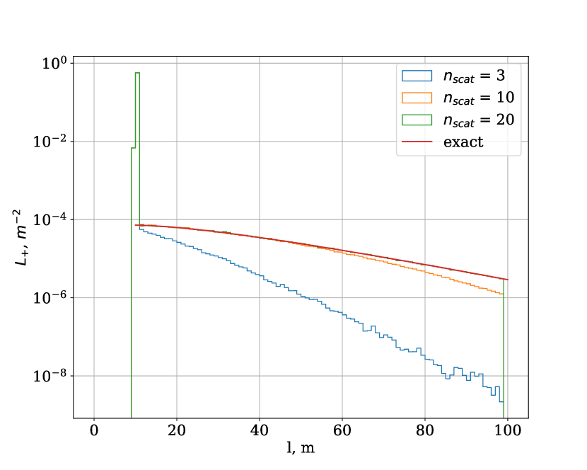
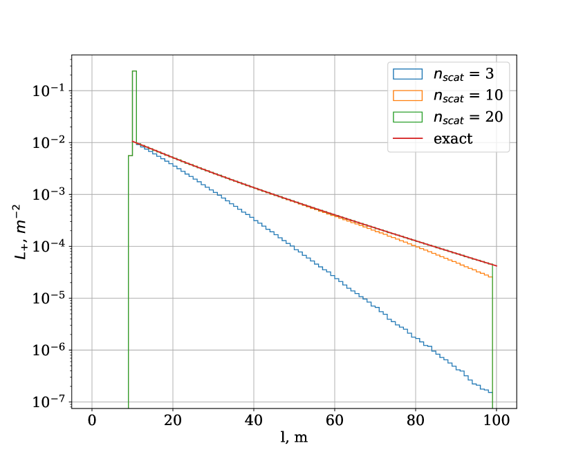
Figure 1: Comparison of the exact solution $L_{+}(l)$, where $l=ct$, (solid line) with the Monte Carlo estimates using $N_{\gamma}=10^{7}$ and $n_{\text{scat}}=3,10,20$, assuming $\mu_{a}=0.05m^{-1}$, $\mu_{s}=0.1m^{-1}$, $x=10\rm{m}$ and $g=0.9$ (upper plot) and $g=-0.9$ (bottom plot).

One can conclude, based on examination of fig. 1, that the Monte Carlo method converges slowly to the exact solution and a dozens of scattering events are required for an accurate estimate of the photon’s flux even for highly forward anisotropy.

III.4 A faster Monte Carlo

An interesting observation is that the exact solution in equation (12) does not depend on $\mu_{s}$ and $g$ separately, but rather on the quantity $\mu^{\prime}_{s}=(1-g)\mu_{s}$. One might wonder if this observation can be used to improve the Monte Carlo algorithm presented earlier. Specifically, one could replace $\mu_{s}$ with $\mu^{\prime}_{s}/2$ and $g$ with some other value. But what value should be chosen for $g$? A plausible guess is that $g=-1$ is the appropriate choice.

Physically, this guess is supported by the fact that an effective inverse scattering length of $(1-g)\mu_{s}$ corresponds to excluding forward scattering, where the direction of a photon remains unchanged. By replacing $\mu_{s}$ with $\mu^{\prime}_{s}/2$, the scattering length becomes longer, but scattering events are still present. In the one-dimensional problem, the only choice available is to change the direction to the opposite direction when such an event occurs. This consideration reinforces the hypothesis that the following replacements are equivalent in the Monte Carlo algorithm:

$$\mu_{s} \to\mu^{\prime}_{s}/2,$$ (25)

$$g \to-1.$$

In appendix B, we prove this statement.

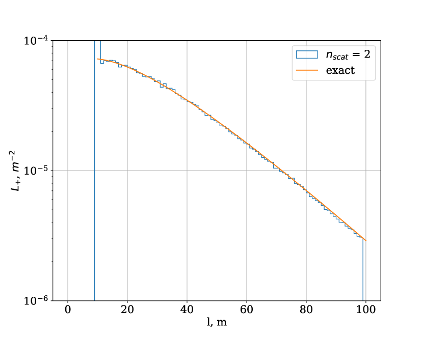
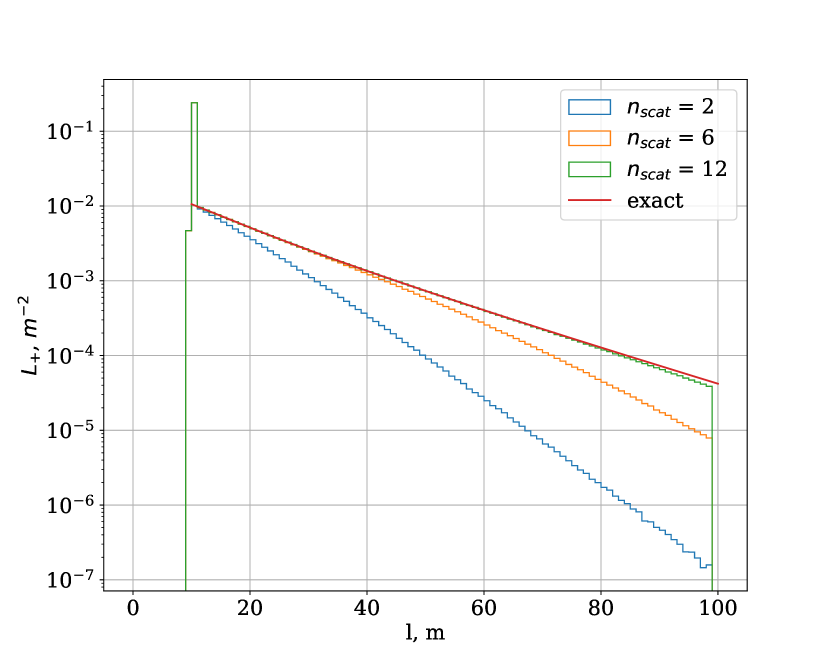
Figure 2: Comparison of the exact solution $L_{+}(l)$, where $l=ct$, (solid line) with the improved Monte Carlo estimates (histograms) using $N_{\gamma}=10^{7}$ and assuming $g=0.9$ (upper, $n_{\text{scat}}=2$) and $g=-0.9$ (bottom, $n_{\text{scat}}=2,6,12$), $\mu_{a}=0.05m^{-1}$, $\mu_{s}=0.1m^{-1}$ and $x=10\rm{m}$.

Although the Monte Carlo algorithm provides equivalent results for both input tuples $(\mu_{s},g)$ and $(\mu^{\prime}_{s},-1)$, the latter demonstrates a much faster convergence rate, as can be observed in the comparison of the Monte Carlo estimates in fig. 2 and the corresponding figure in fig. 1. These figures were generated using the same parameter values for $N_{\gamma}$, $\mu_{a}$ and $\mu_{s}$ and distict asymmetry parameter $g=0.9$ (upper plots) and $g=-0.9$ (bottom plots). A significant increase in the convergence rate can be observed for highly forward scattering ($g=0.9$) where just two scatterings are enough for an accurate estimate of the photon’s flux in the given time domain interval (we remind a reader that $l=ct$). However even for highly backward scattering ($g=-0.9$) the improved version of the Monte Carlo algorithm requires fewer number of scatterings to accurately etimate the photon’s flux: twelth (improved) vs twenty (original). At most extreme case $g=-1$ both Monte Carlo version show identical performance. Therefore, closer asymmetry parameter $g$ approaches to one, fewer scattering are required for the improved version of Monte Carlo.

III.5 Convergence Rate of Monte Carlo Method

Accurately estimating the photon’s flux in a Monte Carlo method requires determining the required number of scattering steps $n_{\text{scat}}$, which can be addressed using the exact solution.

We determine $n_{\text{scat}}$ as follows:

(i) Fix a specific value of the spatial coordinate $x$ expressed in $\mu_{s}^{-1}$.

(ii) Considering the time interval where $l-|x|\leq k\mu_{s}^{-1}$, where $k$ is a free parameter, we require that for any $l\in(|x|,|x|+k\mu_{s}^{-1})$, the following condition holds:

$$|L_{\pm}^{\text{exact}}(l,x)-L_{\pm}^{\text{MC}}(l,x|n_{\text{scat}})|<\varepsilon L_{\pm}^{\text{exact}}(l,x),$$ (26)

Here, $L_{\pm}^{\text{exact}}(l,x)$ represents the exact solution given by eq. 12, and $L_{\pm}^{\text{MC}}(l,x|n_{\text{scat}})$ is the corresponding Monte Carlo approximation that depends on the number of scattering steps $n_{\text{scat}}$. The parameter $\varepsilon$ represents the desired precision. Thus, we estimate $n_{\text{scat}}$ for both the original and faster Monte Carlo algorithms, resulting in two numbers: $n_{\text{scat}}^{orig}$ and $n_{\text{scat}}^{fast}$.

In fig. 3, we present the ratio $n_{\text{scat}}^{\text{orig}}/n_{\text{scat}}^{\text{fast}}$ as a function of the asymmetry parameter $g$ for various values of $k$ and $x$, assuming $\varepsilon=10^{-3}$. This figure illustrates the anticipated trend: a significantly fewer number of steps is required for the faster algorithm as $g\to 1$.

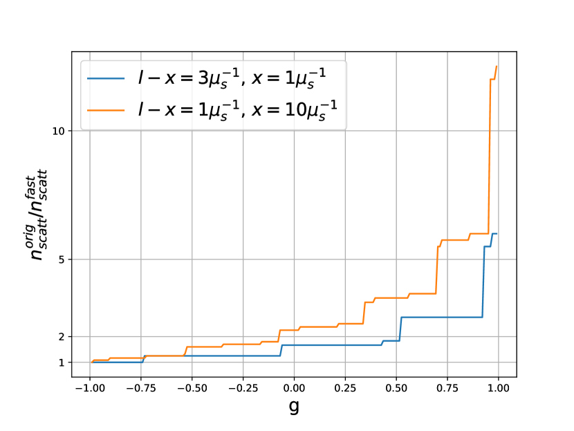
Figure 3: The ratio $n_{\text{scat}}^{\text{orig}}/n_{\text{scat}}^{\text{fast}}$ as a function of the asymmetry parameter $g$ for several values of $k$ and $x$, assuming $\varepsilon=10^{-3}$.

IV Summary

The radiative transfer equation describes how electromagnetic radiation propagates through a medium, and numerical methods are commonly used to approximate its solution. In this paper, we present an exact solution to the one-dimensional time-dependent RTE, which has important practical applications in fields such as atmospheric science, astrophysics, remote sensing, and biomedical optics. The solution is validated using Monte Carlo simulations, and we provide a quantitative analysis of the convergence of the Monte Carlo method to the exact solution.

It is well known that even for highly forward scattering, dozens of random light scatterings are required to obtain an accurate estimate. We demonstrate that a Monte Carlo method with input parameters $(\mu_{s}(1-g)/2,-1)$ can sample photon scatterings much faster than that with $(\mu_{s},g)$ as an input tuple, without sacrificing accuracy. Our study may have implications for other numerical methods used to approximate the RTE.

Interestingly, the exact solution satisfies the Klein-Gordon equation with an imaginary “mass” term, which might suggest a superluminal motion. However, the actual solution is found to be strictly causal.

V Acknowledgements

The authors express their gratitude to the Joint Institute for Nuclear Research for providing financial support for this research. We also appreciate the valuable insights and fruitful discussions contributed by Prof. V. A. Naumov throughout the course of this study.

Appendix A Derivation of solution to one-dimensional RTE

Let us introduce, for the sake of compactness, the differential operators $\hat{K}_{\pm}=\partial_{l}\pm\partial_{x}$. We begin with a guess that $\widetilde{L}_{-}(l,x)$ is actually a function of a single variable $\tau$ defined in eq. 10. Thus, the second eq. 7 reads as follows

$$\widetilde{L}_{+}(l,x)=\frac{1}{\lambda}\hat{K}_{-}\widetilde{L}_{-}(\tau)=\frac{1}{\lambda}\widetilde{L}^{\prime}_{-}(\tau)\frac{l+x}{\tau}.$$ (27)

As one can see, $\widetilde{L}_{+}(l,x)$ is not reduced to a function of $\tau$ only. Substituting eq. 27 into the first eq. 7, one gets

$$\widetilde{L}_{-}^{\prime\prime}+\frac{\widetilde{L}^{\prime}_{-}}{\tau}-\lambda^{2}\widetilde{L}_{-}=0,$$ (28)

which turns out to be a differential equation with the single variable, thus verifying the above assumption.

A solution to eq. 28 is the modified Bessel function of the first order $I_{0}(\lambda\tau)$. However, at $l=0$, this solution does not satisfy the initial condition $\widetilde{L}_{-}(0,x)=0$ since $I_{0}(\lambda\sqrt{-x^{2}})\neq 0$. Multiplying $I_{0}(\lambda\tau)$ by $\widetilde{\theta}(\tau^{2})$ turns out also to be a solution to eq. 28, but it satisfies the initial condition for $\widetilde{L}_{-}$. Lastly, a solution to eq. 28 is determined up to the normalization factor, which we find to be equal to $\lambda/2$:

$$\widetilde{L}_{-}(\tau)=\frac{\lambda}{2}\widetilde{\theta}(\tau^{2})I_{0}(\lambda\tau).$$ (29)

The solution for $\widetilde{L}_{+}$ can be found from the second of eq. 7

$$\widetilde{L}_{+}=\frac{1}{\lambda}\hat{K}_{-}\widetilde{L}_{-}$$ (30)

$$=\frac{1}{2}\left[\left(\hat{K}_{-}\widetilde{\theta}(\tau^{2})\right)I_{0}(\lambda\tau)+\widetilde{\theta}(\tau^{2})\lambda\left(\hat{K}_{-}\tau\right)I^{\prime}_{0}(\lambda\tau)\right]$$

$$=\left[\delta(l-x)+\widetilde{\theta}(\tau^{2})\frac{l+x}{\tau}\frac{\lambda}{2}I_{1}(\lambda\tau)\right],$$

where the following simple relations are handy

$$\hat{K}_{\pm}\tau=\frac{l\mp x}{\tau}=\sqrt{\frac{l\mp x}{l\pm x}},$$ (31)

$$\hat{K}_{\pm}\widetilde{\theta}(\tau^{2})=2\delta(l\pm x).$$

Here we took into account that

$$\frac{dI_{0}}{dx}=I_{1},$$ (32)

$$\frac{dI_{n}}{dx}=I_{n-1}-\frac{n}{x}I_{n}.$$

Finally, we have to make sure that $\widetilde{L}_{+}$ in eq. 30 satisfies the first. of eq. 7

$$\hat{K}_{+}\widetilde{L}_{+}=\left[\hat{K}_{+}\delta(l-x)+(\hat{K}_{+}\frac{l+x}{\tau})\widetilde{\theta}(\tau^{2})\frac{\lambda}{2}I_{1}(\lambda\tau)\right.$$ (33)

$$\left.+\frac{l+x}{\tau}\frac{\lambda}{2}\left((\hat{K}_{+}\widetilde{\theta}(\tau^{2}))I_{1}(\lambda\tau)+\widetilde{\theta}(\tau^{2})\lambda(\hat{K}_{+}\tau)I_{1}^{\prime}(\lambda\tau)\right)\right]$$

$$=\lambda\widetilde{L}_{-},$$

where the following relations are handy

$$\hat{K}_{\pm}\delta(l\mp x)=0,$$ (34)

$$\delta(l\pm x)I_{1}(\lambda\tau)=0,$$

$$\hat{K}_{\pm}\frac{l\pm x}{\tau}=\frac{1}{\tau}.$$

Appendix B Enhancing the Monte Carlo Method

The Monte Carlo algorithm discussed in section III corresponds to the following series:

$$L_{\pm}(l,x)=e^{-(\mu_{a}+\mu_{s})l}\sum_{n=0}^{\infty}\mu_{s}^{n}L^{(n)}_{\pm}(l,x),$$ (35)

where $L^{(n)}_{\pm}(l,x)$ represents the contribution of $n$ scattering events to the photon flux. The form of eq. 35 can be explained as follows: since $l$ is sampled according to the probability density function $e^{-\mu_{s}l}$, this justifies the corresponding exponential factor in eq. 35. The probability of $n$ independent scattering events is proportional to $\mu_{s}^{n}$. Finally, the factor $L^{(n)}_{\pm}(l,x)$ accounts for changes in the photon’s direction during the $n$ scattering events.

The exact solution found in eq. 12 suggests that a Monte Carlo algorithm should have a distinct functional dependence:

$$L_{\pm}(l,x)=e^{-(\mu_{a}+\mu^{\prime}_{s}/2)l}\sum_{n=0}^{\infty}\left(\frac{\mu^{\prime}_{s}}{2}\right)^{n}\widetilde{L}^{(n)}_{\pm}(l,x),$$ (36)

since eq. 12 depends on $\mu^{\prime}_{s}/2$ rather than on $\mu_{s}$ and $g$ separately. By expanding the exact solution as a series of $\mu^{\prime}_{s}/2$ powers, the coefficient functions $\widetilde{L}^{(n)}_{\pm}$ in eq. 36 can be determined. For instance, for the $L_{+}$ function, the coefficients are given by:

$$\widetilde{L}^{(n)}_{+}(l,x)=\begin{cases}\delta(l-x)&\text{for $n=0$}\\ 0&\text{for odd $n$}\\ \widetilde{\theta}(\tau^{2})\sqrt{\frac{l+x}{l-x}}\frac{\tau^{n-1}}{2^{n}(n/2-1)!(n/2)!}&\text{for even $n$}\end{cases}$$ (37)

One can verify that $\widetilde{L}^{(n)}_{\pm}$ does not depend on either $\mu_{s}$ or $g$.

Let us investigate if this series can be obtained from eq. 35 using an appropriate substitution in eq. 25, which was guessed earlier. To demonstrate this, we can start from the exact solution in eq. 12 and rewrite it as:

$$L_{+}=e^{-(\mu_{a}+\mu_{s})l}e^{+\mu_{s}l(1+g)/2}\times$$ (38)

$$\times\left(\delta(l-x)+\widetilde{\theta}(\tau^{2})\sqrt{\frac{l+x}{l-x}}\frac{\mu^{\prime}_{s}}{4}I_{1}\left(\mu^{\prime}_{s}\tau/2\right)\right).$$

Let’s apply the substitution $g=-1$ in eq. 38. Then,

$$e^{+\mu_{s}l(1+g)/2} \to 1,$$ (39)

$$\mu^{\prime}_{s}/2 \to\mu_{s}$$

and

Expanding the $I_{1}$ function in eq. 40 as a series, we obtain the exact form of eq. 36 with coefficients given by eq. 37. This confirms our guess that the Monte Carlo algorithms with input tuples $(\mu_{s},g)$ and $(\mu_{s}(1-g)/2,-1)$ are identical.

To compare the performance improvement of the Monte Carlo algorithm using this simple substitution in eq. 25, the coefficients $L^{(n)}_{\pm}$ in eq. 35 must also be determined for arbitrary $\mu_{s}$ and $g$. Considering $L^{(n)}_{+}$ for definiteness and assuming $g\neq-1$, we find:

$$L^{(0)}_{+} =\delta(l-x),$$ (41)

$$L^{(1)}_{+} =\frac{(1+g)l}{2}\delta(l-x),$$

$$L^{(n)}_{+} =\frac{l^{n}(1+g)^{n}}{2^{n}n!}\delta(l-x)+\widetilde{\theta}(\tau^{2})(l+x)\times$$

$$\times\frac{1}{4}(1-g)^{2}l^{n-2}(1+g)^{n-2}\frac{F_{1}(a_{n},b_{n};2;4z^{2})}{2^{n-2}(n-2)!}$$

where $z=\frac{(1-g)}{2(1+g)}\sqrt{1-\frac{x^{2}}{l^{2}}}$ and $F_{1}(a_{n},b_{n},c,x)$ is the hypergeometric function. The parameters $a_{n}$ and $b_{n}$ are defined as follows.

$$a_{n}=\frac{5-2n+(-1)^{n}}{4},\quad b_{n}=\frac{5-2n+(-1)^{n+1}}{4}.$$ (42)

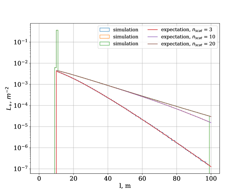
Figure 4: Comparison between the analytic expansion of the exact solution $L_{+}(l)$, where $l=ct$, and the numerical result of Monte-Carlo for $x=10m$ with $g=0,\mu_{a}=0.05m^{-1},\mu_{s}=0.1m^{-1}$.

In fig. 4, we compare the results for $L_{+}$ estimated with the Monte Carlo algorithm discussed in section III to eq. 35, with $L^{(n)}_{+}$ coefficient functions given by eq. 41 for several orders, assuming $g=0$. All terms up to $n$ are summed up in eq. 35 for this comparison. Excellent agreement can be observed, confirming the correctness of eq. 41. One can note that about $n_{\text{scat}}=20$ terms are required to achieve an accurate estimate.

In fig. 5, we display a similar comparison for the improved Monte Carlo as given by eqs. 36 and 37, assuming the same set of parameters.

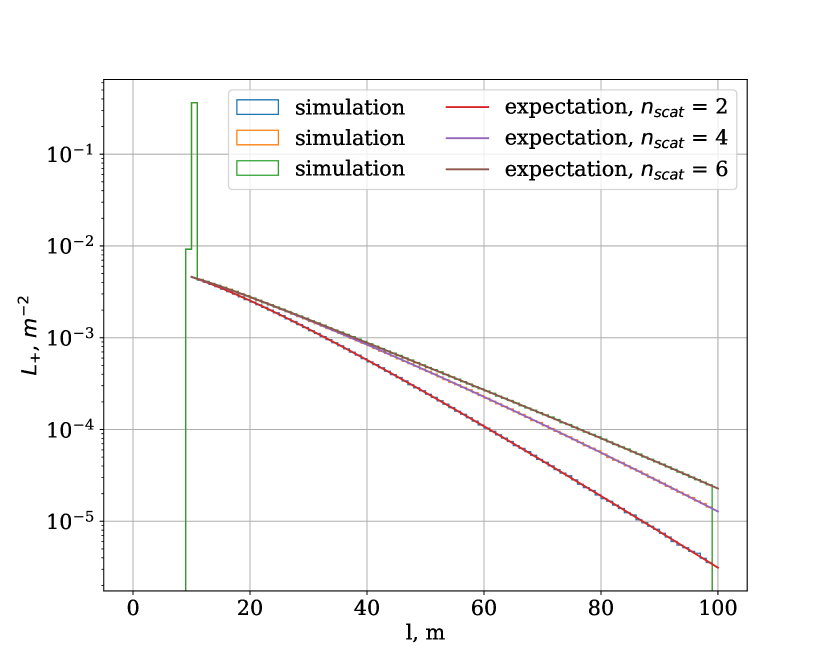
Figure 5: Comparison between the analytic expansion of the exact solution $L_{+}(l)$, where $l=ct$, and the numerical result of improved Monte-Carlo for $x=10m$ with $g=0,\mu_{a}=0.05m^{-1},\mu_{s}=0.1m^{-1}$.

We can conclude that there is excellent agreement between the analytic coefficients in eq. 37 and Monte Carlo expectations, confirming eqs. 36 and 37. Furthermore, we can observe a much faster convergence to the exact solution with the improved Monte Carlo algorithm.

References

- [1] Craig Bohren. Fundamentals of Atmospheric Radiation: an Introduction with 400 Problems. John Wiley & Sons, 2006.
- [2] Jacqueline Lenoble. Radiative Transfer in Scattering and Absorbing Atmospheres: Standard Computational Procedures. A. Deepak Publishing, Hamden, CT, 1985.
- [3] George B. Rybicki and Alan P. Lightman. Radiative Processes in Astrophysics. Wiley-Interscience, 1985.
- [4] Leung Tsang and JA Kong. Radiative transfer theory for active remote sensing of half-space random media. Radio Science, 13(5):763–773, 1978.
- [5] L. V. Wang and H.-I. Wu. Biomedical Optics. Wiley, 2007.
- [6] D. Adamson. The role of multiple scattering in one-dimensional radiative transfer. 1975.
- [7] M. G. Aartsen et al. Observation and Characterization of a Cosmic Muon Neutrino Flux from the Northern Hemisphere using six years of IceCube data. Astrophys. J., 833:3, 2016.
- [8] S. Adrián-Martínez et al. Letter of Intent for KM3NeT 2.0. J. Phys. G, 43(8):084001, 2016.
- [9] Javier Alvarez Sánchez et al. Letter of Intent for the Pacific Ocean Neutrino Explorer (P-ONE). J. Phys. G, 46(11):115103, 2019.
- [10] A. Avrorin et al. The Baikal-GVD Project: Status and Prospects. Universe, 7(9):383, 2021.
- [11] G. Zaccanti et al. Pure and Applied Optics, 3:897, 1994.
- [12] Y. Aharonov, A. Komar, and L. Susskind. Superluminal behavior, causality, and instability. Phys. Rev., 182:1400–1403, Jun 1969.