4D-ONIX: A deep learning approach for reconstructing 3D movies from sparse X-ray projections

Abstract

The X-ray flux provided by X-ray free-electron lasers and storage rings offers new spatiotemporal possibilities to study in-situ and operando dynamics, even using single pulses of such facilities. X-ray Multi-Projection Imaging (XMPI) is a novel technique that enables volumetric information using single pulses of such facilities and avoids centrifugal forces induced by state-of-the-art time-resolved 3D methods such as time-resolved tomography. As a result, XMPI can acquire 3D movies (4D) at least three orders of magnitude faster than current methods. However, it is exceptionally challenging to reconstruct 4D from highly sparse projections as acquired by XMPI with current algorithms. Here, we present 4D-ONIX, a Deep Learning (DL)-based approach that learns to reconstruct 3D movies (4D) from an extremely limited number of projections. It combines the computational physical model of X-ray interaction with matter and state-of-the-art DL methods. We demonstrate the potential of 4D-ONIX to generate high-quality 4D by generalizing over multiple experiments with only two projections per timestamp for binary droplet collisions. We envision that 4D-ONIX will become an enabling tool for 4D analysis, offering new spatiotemporal resolutions to study processes not possible before.

Introduction

X-ray tomography is a non-destructive 3D imaging technique that enables the study of the internal structure and composition of opaque materials [1, 2, 3]. It has been widely applied in various research areas, such as materials science [4, 5], medical imaging [6], biology [7], geology [8], fluid dynamics [9, 10], and also industrial diagnostics [11, 12]. By utilizing X-rays to scan a sample from multiple angles, tomography generates a comprehensive 3D image of the object. The recent advancement of modern Synchrotron Radiation (SR) facilities and X-ray Free-Electron Lasers has opened the way for time-resolved tomography experiments, where exploring dynamics in 4D, i.e., in real-time and in 3D space, has become possible [13]. Time-resolved tomography experiments have demonstrated the capabilities of capturing dynamics with sub-millisecond temporal resolution and micrometer spatial resolution [14, 15]. However, the imaging process of tomography introduces centrifugal forces to the sample during acquisition that can potentially alter or even damage the sample and the dynamics studied. Achieving $1\text{\,}\mathrm{ms}$ temporal resolution would necessitate rotating the sample 500 times per second, generating a substantial centrifugal force that is hundreds of times the gravitational acceleration. This rapid rotation also presents a challenge in developing sample environments that can withstand such speeds. Consequently, the necessary rotation process for collecting a full set of projections often restricts the types of samples that can be used and limits the temporal resolution of X-ray tomography experiments. Additionally, the nature of tomography is not adaptable to single-shot imaging approaches. Various techniques have been developed to overcome this limitation, which aim to achieve higher temporal resolutions while preserving high-quality 3D images of the sample. X-ray Multi-Projection Imaging (XMPI) [16, 17, 18, 19] is developed among others as a time-resolved imaging technique. Unlike conventional scanning-based techniques, XMPI records volumetric information without scanning by generating different beamlets that illuminate the sample simultaneously from different angles. By combining the concept of XMPI with the unique capabilities of the fourth generation SR sources [20, 21] and XFELs [22], one can record 3D information of dynamical processes from kHz [23, 24] up to MHz rate [25], exploiting the possibility of imaging 3D using single-pulses of XFELs. This opens up new possibilities for studying the high-speed dynamics of various materials. However, unlike tomography which records hundreds of projections of a sample, XMPI records no more than eight projections due to practical constraints [16, 18, 24], and a reconstruction algorithm is required to recover 4D (3D + time) information from the extremely sparse data collected from XMPI.

It is unlikely to solve this problem using traditional methods due to the highly ill-defined nature of the problem [26]. Recent advancements in DL approaches provide a potential solution to this problem. DL algorithms, such as Convolutional Neural Networks [27] and Generative Adversarial Networks [28], can be trained to learn the underlying structure of the sample and produce high-quality reconstructions from sparse inputs [29, 30, 31]. Specifically, approaches based on Neural Radiance Fields (NeRF) [32] have recently shown promise in optical and X-ray imaging for reconstructing high-resolution 3D / 4D structures from sparse views [33, 34, 35, 36, 37, 38, 39]. Instead of relying on voxels, these methods learn the shape of an object as an implicit function of the 3D spatial coordinates, offering a potential solution to the longstanding memory issues associated with 3D reconstructions. The recently developed ONIX algorithm showed the 3D reconstruction from eight views for the experimental and simulated tomographic experiments [36]. However, there is a need for a 4D reconstruction algorithm to investigate ultrafast dynamical processes using highly sparse X-ray projections acquired through XMPI.

Here we report 4D-ONIX, a self-supervised DL model that learns to reconstruct high-quality temporal and spatial information of the sample from the extremely sparse projections collected with XMPI. It does not require 3D ground truth or prior dynamic description of the sample at any stage - neither during the training nor during its deployment. Once trained, it can reconstruct a 3D movie showing the refractive index of the sample as a function of time from only the recorded projections. The capability of 4D-ONIX is achieved by i) incorporating the physics of X-ray propagation into the model, ii) having a continuous representation of the sample that describes the refractive index as a function of position and time, iii) learning the latent features of the sample by generalizing over all timestamps, and iv) applying adversarial learning to enforce consistency between measured and predicted projections. We demonstrate our approach to dynamical processes of binary water droplet collisions [40, 41, 42]. We validate the performance of our approach using simulated droplet collision datasets modeled using the Navier-Stokes Cahn-Hilliard equations [43, 44]. Volumetric information of binary droplet collision was retrieved from two projections of simulated XMPI experiments. This approach has also been applied to experimental XMPI data collected at European Synchrotron Radiation Facility (ESRF) and European X-Ray Free-Electron Laser Facility (European XFEL) with kHz up to MHz acquisition rates  [24, 25]. We envision that 4D-ONIX will be pivotal for the implementation and applications of XMPI, and it will enable new spatiotemporal resolutions for time-resolved 3D X-ray imaging through novel acquisition approaches based on sparse projections. The 4D reconstructions offered by 4D-ONIX will provide valuable observations for in-situ and operando testing for a plethora of systems, e.g., the characteristics and dynamic studies in fluid dynamics and material science, which are important for various applications such as the study of atmospheric aerosols [45, 46], advancements in fuel cell technologies [47] and improvements in additive manufacturing [48, 49, 50, 51]. It is worth mentioning that our approach can also be extended to single-shot phase contrast imaging [52, 53, 54] and coherent diffraction imaging [55, 56] experiments where the propagation model is explicitly known. Furthermore, the availability of 4D reconstruction from 4D-ONIX opens up the possibility of directly constraining the dynamics in the reconstruction process, e.g., through the use of Physics-Informed Neural Networks [57].

Results

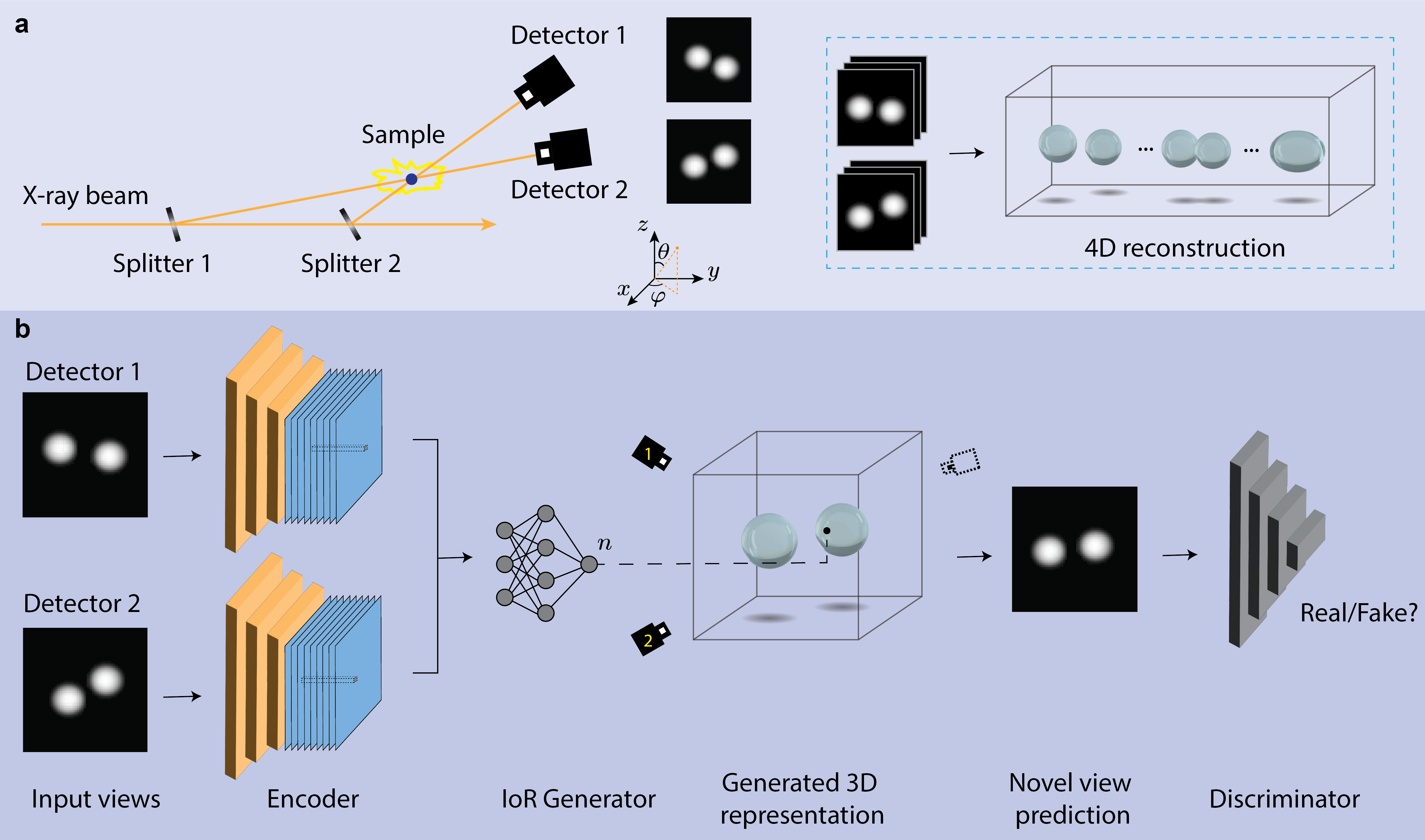
Figure 1: Demonstration of XMPI experiment and the reconstruction approach. a Conceptual illustration of the XMPI setup. The dashed blue box on the right shows the goal of the reconstruction approach. b Overview of the 4D-ONIX approach.

Concept of XMPI and overview of the approach

The concept of XMPI is depicted in Figure 1 a. Unlike tomography measurements which rotate the sample in a period of 180° or 360° and record, typically, hundreds to thousands of projections in between, the measurement of XMPI does not require rotations of the sample. XMPI relies on high-brilliance X-ray sources and a group of beam splitters to generate multiple beams that illuminate the sample simultaneously from different angles and a set of kHz/MHz detectors to record the different sample projections. In this way, one can record volumetric information on the fast dynamics of the sample, ultimately limited by the speed of the detector and the flux of the X-ray source. Inset marked by the blue box of Figure 1 a shows the goal of XMPI, which is to achieve a continuous 3D movie of the sample being studied from the projections recorded, exploiting excellent temporal characteristics provided by XFELs or the fourth-generation SR sources. This opens up possibilities for observing in 3D kHz up to MHz dynamics of the sample. As shown in Figure 1 a, the data used here comes from applying XMPI to water droplet collisions using two split beamlets.

We designed a self-supervised DL algorithm, 4D-ONIX, to reconstruct temporal and spatial information from XMPI. It combines neural implicit representation [32] and generative adversarial mechanism [28] with the physics of X-ray interaction with matter, resulting in a mapping between the spatial-temporal coordinates and the distribution of the refractive index of the sample. By enforcing consistency between the recorded projections and the estimated projections generated by the model, the model learns by itself the 3D volumetric information of the sample at each measured time point from only the given projections without needing real 3D information about the sample. Once trained, it provides a 3D movie showing the structure and dynamics of the sample.

Self-supervised 4D reconstruction approach

The architecture of the self-supervised 4D reconstruction model (4D-ONIX) is depicted in Figure 1 b. The goal of the model is to learn the Index of Refraction (IoR) of the sample at any spatial-temporal point. The 4D-ONIX model is based on three neural networks: an encoder, a 4D IoR (index of refraction) generator, and a discriminator. The encoder and the discriminator are built up on CNNs, whereas the IoR generator is formed by fully connected Multilayer Perceptrons. The IoR generator learns the local features of each object, while the encoder and the discriminator capture both the local features and global features across all timestamps and experiments. The recorded projections are first sent into the encoder, which interprets the images (2D) into stacks of downscaled feature maps (3D). For each spatial-temporal point, feature encoding was performed in the camera space where we applied an affine coordinate transformation to transfer from the global coordinate system to the local coordinate system of each view. The IoR generator receives extracted feature maps from the encoder and predicts the value of the index of refraction at each spatial point. In this way, we can predict the value of the index of refraction of the sample at any spatial-temporal point. Please note that the IoR generator relies on neural implicit representation which learns a continuous function of the refractive index, which differs from many common 3D reconstruction approaches that learn the value of each isolated voxel. We apply a physics-based forward propagation model to predict projections from different angles in the plane of incoming X-rays. The forward model is based on the projection approximation (weak scattering) [58], where secondary scattering caused by the X-ray photons is ignored. Note that this can also be extended to multiple scattering conditions by using multi-slice methods [58]. The discriminator constrains the predictions by differentiating them from the real ones and minimizing the differences between them. The networks are trained by an adversarial loss function. We use the same encoder, generator, and discriminator for the training of the sequence of all 3D movies. Therefore, the networks are trained by all of the recorded projections so that these networks, especially the convolutional layers in the encoder and the discriminator, learn generalized features across the whole sequence. Further details of the network implementation and the loss function are included in the 4D-ONIX algorithm and Network and training details sections.

4D-ONIX performance evaluation

We assess the performance of 4D-ONIX using simulated datasets of droplet collisions modeled with the Navier-Stokes Cahn-Hilliard equations. We refer the readers to the Simulation of water droplet collision section for details about the droplet collision simulation. The simulations provided multiple sequences of 3D objects, each sequence illustrating the collision process between two water droplets. Two projections were generated from each 3D object to mimic the experimental conditions of the XMPI experiment performed at the European XFEL [25]. For brevity, we refer to each collision sequence as an XMPI experiment or simply an experiment. The geometry of the projection generation in the simulated XMPI experiment is illustrated in Figure 2 a. We evaluate 4D-ONIX using the simulated datasets under two scenarios, as visualized in Figure 2 b.

1. Reproducible processes. It involves multiple identical experiments of the same dynamical process; as shown in Figure 2 b, the samples may exhibit a variety of orientations throughout the experiments. This can arise from various factors such as random sample orientations, samples arriving from different directions, or manual rotation of the sample stage. For instance, assuming we set the projection from detector 1 of the first experiment as $0\mathrm{°}$ and denote the relative angle between the two projections as $\Delta\varphi$, in the first experiment, the dynamics process is measured at $\varphi_{1}=$$$ and $\varphi_{2}=\Delta\varphi$. In the second experiment, the sample orientation is shifted by $\phi=$$$, and the two projections are measured at $\varphi_{1}^{\prime}=$$$ and $\varphi_{2}^{\prime}=$$+\Delta\varphi$. The third experiment can be measured at $\varphi_{1}^{\prime\prime}=$$$ and $\varphi_{2}^{\prime\prime}=$$+\Delta\varphi$, and so on. This allows for obtaining volumetric information of the collision process from different angles of the sample without rotation.

2. Quasi-reproducible processes. In many cases, measuring perfectly reproducible processes is challenging or impractical. It is more realistic to measure several experiments capturing similar dynamical processes within experimental tolerances, with each process being measured only once — resulting in only one 4D sequence available for each process. As illustrated in Figure 2 b, similar to the first scenario, the dynamical processes are measured from different orientations. However, the dynamical processes themselves are not identical. For example, in the first experiment, both droplets have the same size, whereas in the second experiment, one droplet is larger than the other. In the third experiment, the droplets may be moving faster than in the first experiment, and so forth.

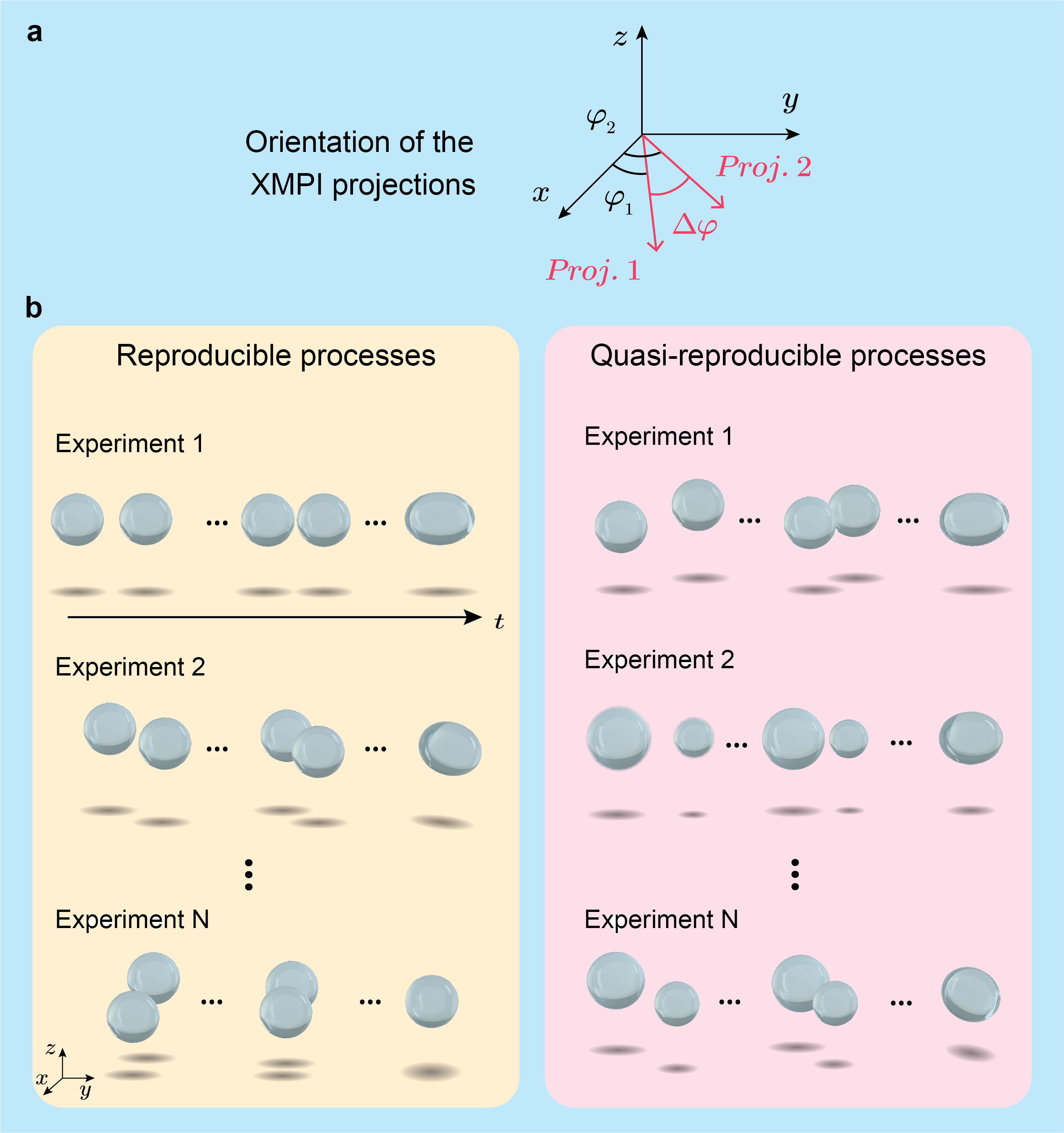
Figure 2: Demonstration of the simulated XMPI data. a Geometry of the simulated XMPI projections. Projection pairs are generated on the x-y plane with a fixed angle between them. b Comparison of the two training scenarios. In the reproducible processes scenario, the processes are identical, while in the quasi-reproducible processes scenario, dynamical processes can differ. For example, the size of droplets may vary among experiments, as shown here.

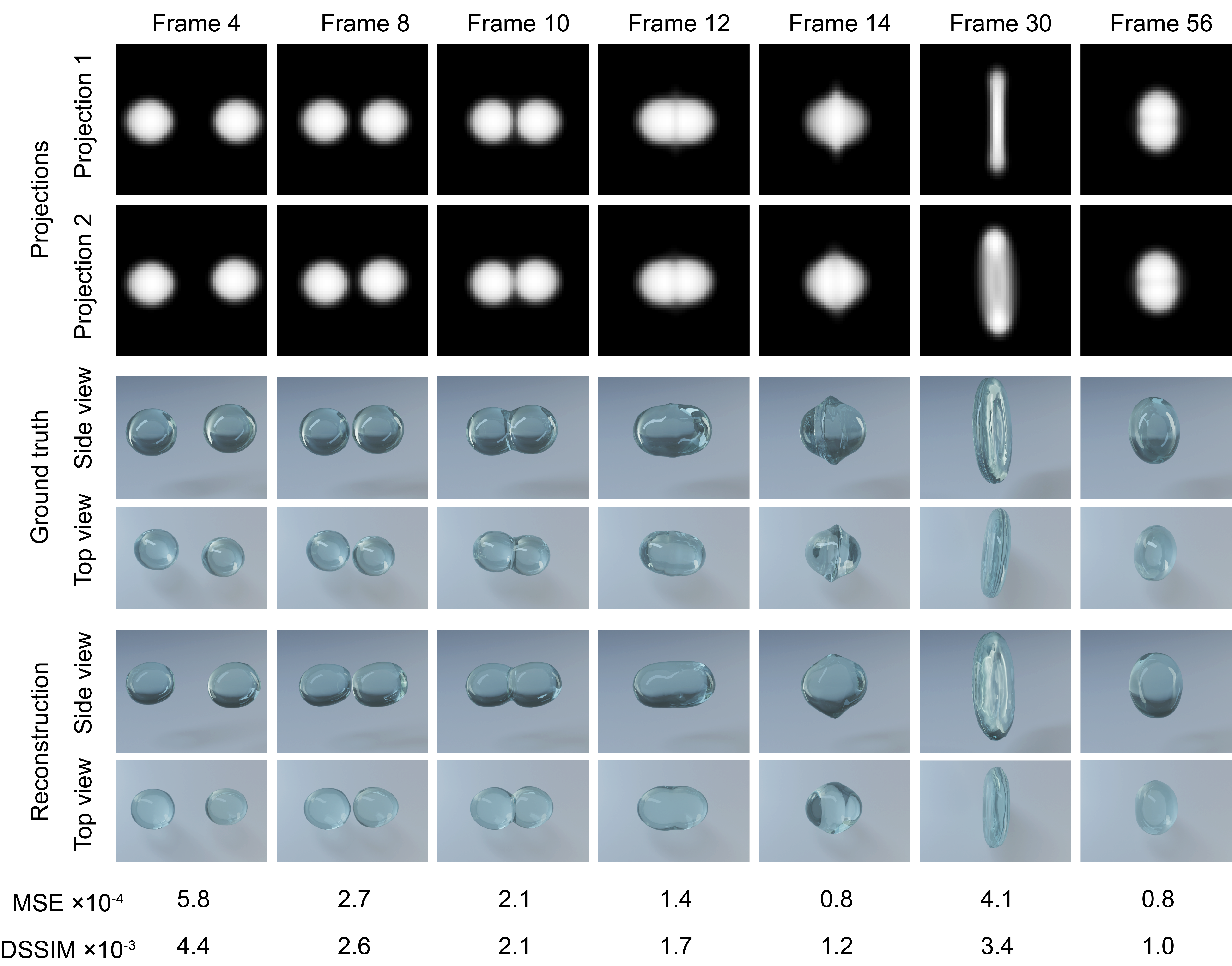
Figure 3: Demonstration of the 4D reconstruction for a reproducible process. Seven timestamps are shown, illustrating different stages of the droplet collision process. The two generated projections are shown in rows 1-2, corresponding to $0\mathrm{°}$ and $23.8\mathrm{°}$, respectively. The top view and side view of the 3D ground truth are shown in rows 3-4. The top and side views of the 4D-ONIX reconstructions are shown in rows 5-6. The bottom two rows show the MSE and DSSIM between the 4D-ONIX reconstruction and the ground truth for each corresponding timestamp.

Two training datasets were generated for the two scenarios. The first dataset was based on a single simulation, mimicking 16 experiments of a reproducible process. Each experiment contains a pair of projections with random $\varphi$ angles and fixed $\Delta\varphi$ for each timestamp. The second dataset was simulated for quasi-reproducible processes. It was based on 16 simulations, where a single projection pair with random orientation of the sample was selected from each simulation to form a training dataset. All 16 simulations simulated the collision process of binary droplets, with 10% variance in collision velocities and 10% variance in droplet size based on the tolerance of the droplets collision experiment conducted at European XFEL [25]. For both datasets, the relative angle between the projection pairs was selected as $23.8\mathrm{°}$ to match the experimental conditions of the XMPI setup at the European XFEL [25]. Each simulation contained 75 timestamps, and both datasets contained 1200 timestamps in total.

We trained 4D-ONIX with different numbers experiments, from 1, 2, 4, 8, to 16, for both scenarios. The reconstruction results and their quality improvement as a function of increasing the number of experiments are presented in the Supplementary Information. Here, we only present the best results trained with 16 experiments. First, we present the results of training with reproducible processes. Figure 3 shows examples of the 4D-ONIX performance trained on reproducible processes. It shows the two projections, the 3D of the ground truth and the reconstruction rendered from the side and top views. The side view corresponds to the x-axis, while the top view aligns with the z-axis, which is perpendicular to the acquisition plane. Seven timestamps are shown, demonstrating the crucial stages in the collision process for one of the collision experiments. In this collision experiment, two identical water droplets were accelerated and collided center-to-center at the same speed. A full movie of the reconstruction is provided in Supplementary Information. Please note that the 3D ground truth shown here was only used for comparison, and they were never shown to the network at any stage. The reconstructions were quantified by Mean Squared Error (MSE) and Dissimilarity Structure Similarity Index Metric (DSSIM) [59], and their values for selected timestamps are shown in Figure 3. Both of the metrics calculate the difference between the 4D-ONIX reconstructions and the ground truth. Therefore, a value closer to zero indicates a better reconstruction. Furthermore, we analyzed the evolution of errors throughout the collision process for each 3D timestamp, with the results displayed in Figure S1 (Supplementary Information). In addition to 3D metrics, we also computed metrics in the 4D domain. We calculated the 4D MSE and 4D DSSIM for all 75 timestamps of the demonstrating experiment, resulting in MSE=$2.6\times 10^{-4}$ and DSSIM=$2.3\times 10^{-3}$. Apart from evaluating data correlation in the object space, we also evaluated the performance of the reconstructions in the frequency space using Fourier Shell Correlation (FSC) and Fourier Ring Correlation (FRC) [60, 61]. FSC and FRC calculate the normalized cross-correlation between the reconstructions and the ground truth in frequency space over shells (3D) and rings (2D), respectively. The resolution of the reconstructions can be retrieved from the correlation curves. Here, we used the half-bit threshold criterion for resolution determination. The retrieved 3D spatial resolution was 4 $\pm$ 1 voxels, with the voxel side size being equivalent to the pixel size of the input projections. The 2D resolution was separately calculated for the training views and unseen views. For the unseen views, resolution was 6.0 $\pm$ 1.6 pixels, while for the training views, it was 4.7 $\pm$ 1.6 pixels. Please refer to Figure S2 (Supplementary Information) for the plots of FSC and FRC for example timestamps.

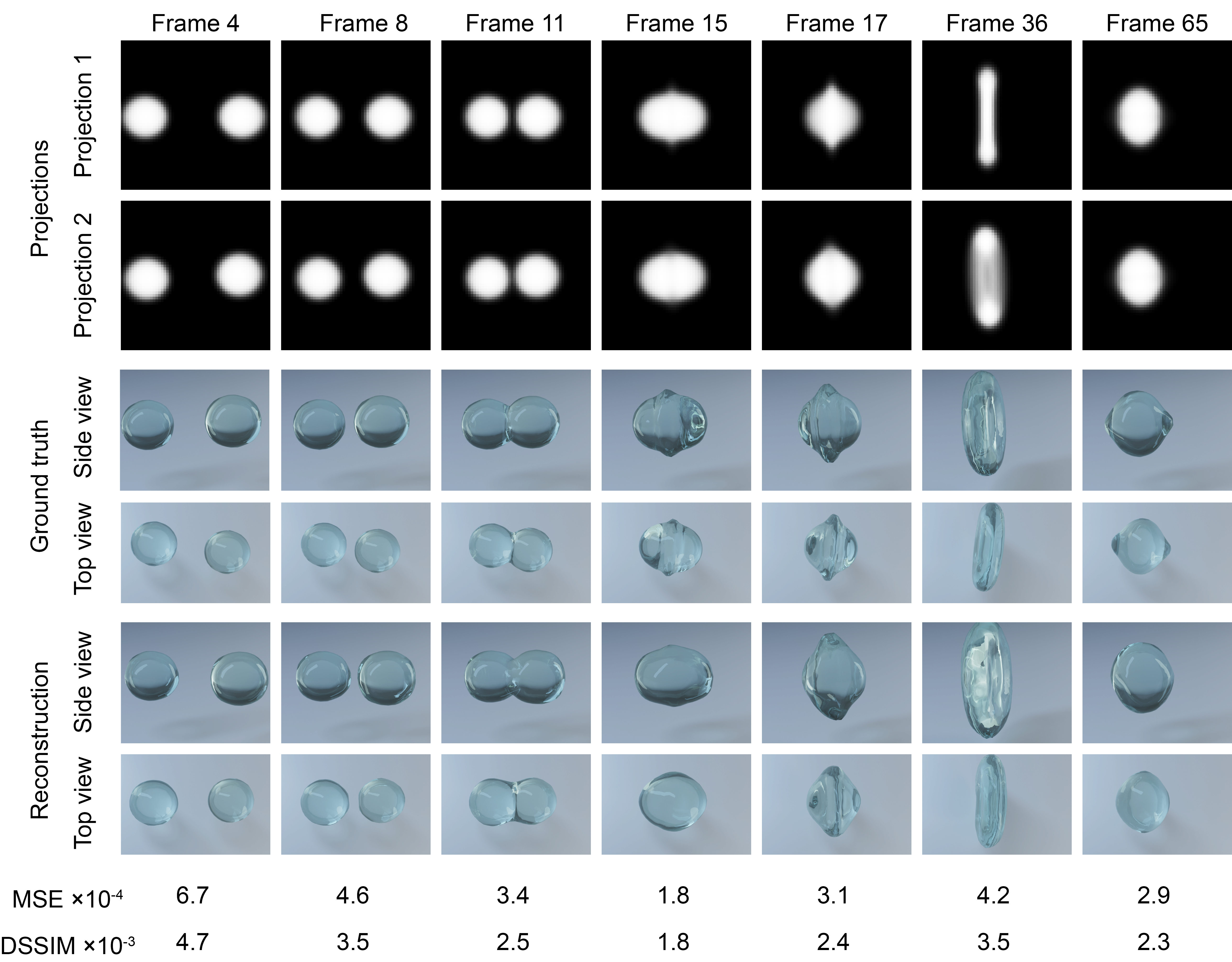
Figure 4: Demonstration of the 4D reconstruction for a quasi-reproducible processes. In this demonstrating experiment, the droplet on the right is bigger and moves faster than the one on the left. The seven timestamps shown here depict different stages of the droplet collision process. The two projections are shown in rows 1-2, corresponding to $0\mathrm{°}$ and $23.8\mathrm{°}$, respectively. The top view and side view of the 3D ground truth are shown in rows 3-4. The top and side views of the 4D-ONIX reconstructions are shown in rows 5-6. The bottom two rows show the MSE and DSSIM between the 4D-ONIX reconstruction and the ground truth for each corresponding timestamp.

Second, we present the results obtained from training with the dataset of quasi-reproducible processes, comprising multiple simulations featuring similar but not identical samples. Figure 4 demonstrate the performance of 4D-ONIX trained on quasi-reproducible processes. Analogously to the reproducibility test, the figure presents the two projections, the 3D representation of the ground truth, and the reconstruction rendered from side and top views, providing a representation of the collision process between two water droplets. A full 3D movie of the reconstruction can be found in the Supplementary Information. In this specific experiment, one of the water droplets (the one on the right) was 7% larger than the other, and the larger droplet also moved 7% faster than its counterpart. The 4D metrics for the reconstructions were calculated, resulting in MSE=$4.3\times 10^{-4}$ and DSSIM=$3.2\times 10^{-3}$. The distribution of errors throughout the collision process for each timestamp is visualized in Figure S1 (Supplementary Information). We determined the 3D spatial resolution using FSC, resulting in a resolution of 6 $\pm$ 1 voxels. The 2D resolution was found to be 7 $\pm$ 2 pixels for the training views and 10 $\pm$ 4 pixels for the unseen views. Please refer to Figure S4 (Supplementary Information) for additional figures of FSC and FRC.

Discussion

We have demonstrated the application of 4D-ONIX, a self-supervised DL 4D reconstruction model to reconstruct 4D data of water droplet collisions using simulated XMPI datasets. We evaluated the performance of 4D-ONIX under two scenarios: with reproducible processes and with quasi-reproducible processes. As depicted in Figure 3 and Figure 4, we reconstructed 3D movies of water droplet collision using 16 experiments. Each experiment contained only two 2D projections over 75 different timestamps. The reconstructions accurately captured the dynamics of the water droplet collision process. Even the top view, which was perpendicular to the projection plane, was effectively reconstructed. This view was experimentally unobservable and never shown to the networks. We evaluated the MSE, DSSIM, and the resolution of the reconstructions. The MSE was $2.6\times 10^{-4}$ for the training with reproducible processes and $4.3\times 10^{-4}$ for the training with quasi-reproducible processes. The DSSIM was $2.3\times 10^{-3}$ and $3.2\times 10^{-3}$ for the training with reproducible and quasi-reproducible processes, respectively. This suggests that our approach effectively reconstructs the collision processes of the water droplets. The ability to reconstruct 3D from two projections is largely attributed to 4D-ONIX’s capacity to generalize across all timestamps of various experiments using an encoder. Furthermore, 4D-ONIX learns not only the self-consistency of the two projections in 3D but also the shared features of the samples through the discriminator. Regarding the resolution of the 3D reconstructions, 4D-ONIX achieved a resolution of approximately 4 voxels for training with reproducible processes and 6 voxels for training with quasi-reproducible processes. Further investigation found that the reconstructions had a superior resolution for the trained views over unseen views for both scenarios. This is mainly due to the fact that the projections were only recorded in the plane formed by the two beamlets, providing very limited information from the top. As shown in Figure 3, Figure 4, and Figure S1, the error distribution with time suggested that the timestamps prior to the collision process appear to be more difficult to reconstruct. This difficulty may come from the distortion of the droplets induced by the acceleration process within the simulation and the inadequacy of training data available for this particular stage. Comparing the training results between reproducible and quasi-reproducible processes, it is observed that the training shows better performance for reproducible processes than quasi-reproducible processes. Learning the features of a single experiment is a less complex task than generalizing across multiple experiments with different parameters within the experimental tolerance. Introducing multiple experiments may introduce additional variability and complexity, making it more challenging for the networks to capture and reconstruct essential features. Nevertheless, obtaining reproducible samples or processes is not always guaranteed, making quasi-reproducible processes a more common scenario and closer to experimental conditions. We also conducted comparisons by training 4D-ONIX with different numbers of experiments, and the corresponding metrics for the reconstructions are detailed in Table S1 and Table S2. The results indicated that the performance was less favorable with 1-2 experiments, but improved greatly when more than 4 experiments were available. Reconstructions with fewer than four experiments may lead to a range of diverse and incorrect solutions for the sparse-view reconstruction problem. This variability, particularly noticeable in the top view (the unseen view), resulted in reconstructions that deviated from the ground truth, as illustrated in Figure S3 and Figure S5. Our results with water droplet collision demonstrated that 16 experiments were adequate for training an accurate model. For more complicated processes, more experiments may be needed to achieve satisfactory results.

4D-ONIX has also been applied to experimental data collected at European XFEL, where collisions of binary droplets were recorded at 10 keV in 1.128 MHz frame rate using XMPI with two split beamlets [25]. 4D-ONIX can reconstruct a complete 3D movie capturing the collision of water droplets from the experimental XMPI dataset, using just two projections for each dynamical process. The temporal resolution of the 3D movie retrieved was $0.89\text{\,}\mathrm{\SIUnitSymbolMicro s}$, which is three orders of magnitude faster than state-of-the-art time-resolved tomography [15]. Unfortunately, the retrieved reconstructions may suffer from imperfections as i) only two sequences of the droplet collision were captured, with a minimal shift in sample orientation ($23.8^{\circ}$), and ii) the recorded projections suffered from noise and imaging artifacts.

4D-ONIX is a data-driven approach, and its performance is determined by the quality and quantity of the training dataset. In this work, 4D-ONIX has been trained using just two projections, which is an extremely ill-posed problem that can limit the accuracy of the reconstruction. Setups of XMPI have also been demonstrated on SR sources at Super Photon Ring – 8 GeV (SPring-8) in Japan and ESRF in France, which generate more than two projections and can capture dynamical processes at sub-millisecond timescales with $\sim$ $10\text{\,}\mathrm{\SIUnitSymbolMicro m}$ spatial resolution [23, 24]. These extra projections as well as increasing the angular separation between projections ($\Delta\varphi$) can improve the performance of 4D-ONIX and reduce the number of experiments required to satisfactorily reconstruct 4D information. Thus, such advancements in XMPI will improve 4D-ONIX’s performance. The number of experiments is a crucial factor that affects the accuracy of the reconstruction. We have evaluated its effect for this specific scientific case, as illustrated in Figures S1, S3, and S5. One can observe that the model’s efficacy may be compromised when trained with only one or two experiments. Increasing the number of experiments for identical or similar samples is key to improving both convergence and the accuracy of the reconstructions. This way, the neural networks receive more information about the sample, contributing to improved model performance. Up to this point, our approach has been validated on water droplets. With advancements in the experimental setup and increased availability of training datasets, it should be feasible to extend our reconstruction capabilities to more complex samples, such as metallic foams [15] or additive manufacturing [48].

The 4D nature and the inclusion of X-ray physics in 4D-ONIX offer opportunities for further development. First, the temporal information available from 4D-ONIX’s reconstructions provides opportunities for improvement by introducing additional constraints. For instance, if the sample dynamics adhere to a Partial Differential Equation (PDE), incorporating an extra PDE loss term into the loss function using PINNs [57] can not only better align the model with the laws of physics but also facilitate the interpolation between the dynamical processes. This will enable the generation of a continuous 3D movie with temporal resolution surpassing the recording rate of the XMPI experiment. Furthermore, the inclusion of a frame variation regularizer can further improve the reconstruction quality [35]. The 4D-ONIX code provides the option to include a frame variation regularizer in the time domain, minimizing the variance of adjacent timestamps. This can be particularly beneficial when dealing with high temporal resolutions or rapidly evolving samples. Second, 4D-ONIX offers adaptability and flexibility to be applied to other types of time-resolved imaging experiments, such as coherent diffraction imaging [55, 56] and phase-contrast experiments [52, 53, 54]. The propagation and interaction model implemented in 4D-ONIX can be readily adapted to suit different experiments’ specific imaging formation processes, e.g., to directly perform 4D phase reconstructions.

In conclusion, we have presented 4D-ONIX, a novel physics-based self-supervised deep learning approach capable of reconstructing high-quality temporal and spatial information of the sample from extremely sparse projections. 4D-ONIX provides an innovative solution for single-shot time-resolved X-ray imaging techniques like XMPI, which rely on recording a sparse number of sample projections simultaneously to avoid the scanning processes, as used in X-ray tomography. With the application of 4D-ONIX on simulated XMPI data of water droplet collision, we have demonstrated the capacity of our approach to reconstruct high-resolution 3D movies from only two projections per timestamp, preserving the critical dynamics of the observed phenomenon. We envision that 4D-ONIX will open up unprecedented possibilities for more sophisticated time-resolved X-ray imaging experiments and push the limits of time-resolved imaging when combining the use with XMPI and advanced high-brilliant X-ray sources such as the fourth-generation SR sources and XFELs. The reconstructions provided by 4D-ONIX will allow for an in-depth exploration of rapid physical phenomena in fluid dynamics and material science, potentially impacting fields like atmospheric aerosol research and additive manufacturing. Additionally, the self-supervised learning approach demonstrated by 4D-ONIX has the potential to provide new spatiotemporal resolutions through novel acquisition approaches that only acquire a sparse number of projections. Finally, the possibility to directly reconstruct 3D processes provides a framework to implement physics-based methods for dynamic studies.

Methods

Simulation of water droplet collision

Consider the domain $\Omega$ and time $t\in(0,T]$, denote $\Omega_{T}=\Omega\times(0,T]$. In this paper, we use $\psi\in[-1,1]$ as the phase variable, with $\psi=1$ to label phase $1$ (i.e. water) and $\psi=-1$ to label phase $2$ (i.e. air), and $\psi\in(-1,1)$ representing the interface.

Consider the non-dimensional Reynolds and Weber numbers defined as

$$Re:=\frac{\rho_{r}UL}{\mu_{r}}\quad\text{ and }\quad We:=\frac{\rho_{r}U^{2}L}{\sigma}\quad,$$ (1)

with $U$ the characteristic velocity, $L$ the characteristic length scale, $\sigma$ the surface tension and $\rho_{r}=\rho_{1}$ and $\mu_{r}=\mu_{1}$ as the reference density and viscosity for non-dimensionalization.

Following [43, 44], using volume averaged densities and viscosities

$$\rho(\psi)=\frac{1}{2}\big{(}(1+\psi)\rho_{1}+(1-\psi)\rho_{2}\big{)}\quad\text{ and }\quad\mu(\psi)=\frac{1}{2}\big{(}(1+\psi)\mu_{1}+(1-\psi)\mu_{2}\big{)}$$ (2)

the fluid flow is described by the incompressible Navier-Stokes equations in non-dimensionalized form with potential surface tension $\eta\nabla\psi$

$$\rho(\psi)\big{(}\partial_{t}\mathbf{u}+\mathbf{u}\cdot\nabla\mathbf{u}\big{)}-\frac{\mu(\psi)}{Re}\nabla\cdot\nabla\mathbf{u}+\nabla p =-\frac{1}{We}\eta\nabla\psi \quad\mbox{ in }\Omega_{T},$$ (3)

$$\nabla\cdot\mathbf{u} =0 \quad\mbox{ in }\Omega_{T},$$ (4)

with an appropriate combination of boundary conditions for velocity $\mathbf{u}$ and pressure $p$.

The movement and shape of the interface is described by the Cahn-Hilliard equations, given the double well potential $W(\psi)=\frac{1}{4}(\psi^{2}-1)^{2}$ and thus $\partial_{\psi}W(\psi)=(\psi^{2}-1)\psi$:

$$\partial_{t}\psi+\nabla\cdot(\mathbf{u}\psi-\omega\nabla\eta) =0\quad\mbox{ in }\Omega_{T}$$ (5)

$$\eta-\partial_{\psi}W(\psi)-\varepsilon^{2}\Delta\psi =0\quad\mbox{ in }\Omega_{T}$$ (6)

where $\psi$ is the phase variable, $\eta$ the chemical potential, and $\omega$ a mobility parameter and $\varepsilon$ is an artificial parameter describing the interface thickness. The equations are, in our case, equipped with natural boundary conditions.

Similar to [44], low-order Finite Element techniques are used to discretize the Navier-Stokes Cahn-Hilliard equations. For the Navier-Stokes equations (3),(4) a pressure-correction projection method with second order backward differencing formula (BDF2) in time, described in [62], and a Taylor-Hood conforming Finite Element pair $(\mathbb{P}_{2},\mathbb{P}_{1})$ for $(\mathbf{u},p)$ in space are used. For the Cahn-Hilliard equation (5),(6) a conforming Finite Element pair $(\mathbb{P}_{1},\mathbb{P}_{1})$ for $(\psi,\eta)$ and Crank-Nicholson in time with mass lumping is used. The equations are decoupled by solving sequentially first the interface motion using the velocity from the previous time step followed by a Navier-Stokes solve using the updated phase variable. This works well for reasonably small time steps. The resulting linear systems are solved with a (S)SOR preconditioned GMRes or CG method from the DUNE-ISTL module [63] with a tolerance of $10^{-8}$. To reduce the computational effort, mesh adaptation based on the newest vertex bisection is applied [64, 65]. The refinement indicator is based on the phase variable $\psi$ and defined as $\theta(\psi)=2(\psi+1)(1-\psi)$. A mesh element is refined when $\theta(\psi)>0.15$ and coarsened whenever $\theta(\psi)<0.0525$. The implementation is done in the open-source framework DUNE and in particular DUNE-FEM [66, 67] using the Python based user interfaces, which allows the description of weak forms using UFL [68].

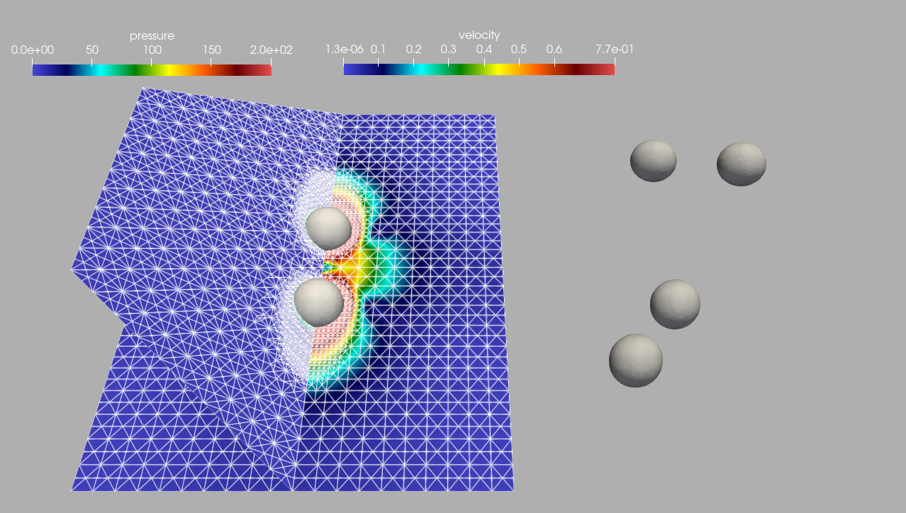
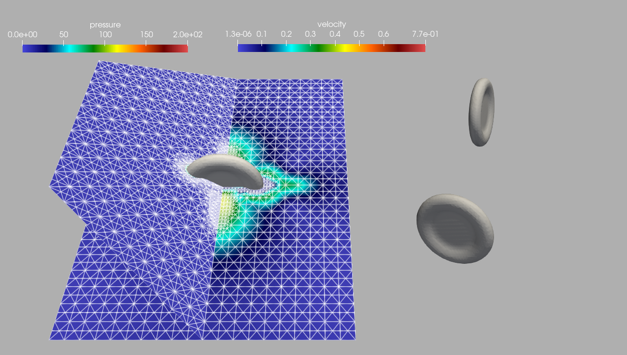
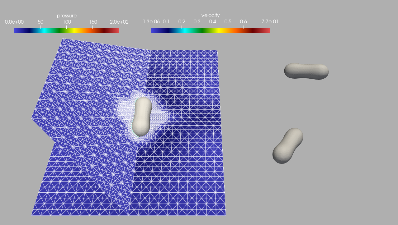
Figure 5: Equal sized centered collision of two droplets viewed from different angles. Dynamic grid adaptation is used which reduces the computational effort by a factor of $40$.

For the simulations carried out in this work, parameters resembling the experiment were used. In particular, $Re=200$, $We=6.94$, $U=2.5\,m/s$, $L=8\cdot 10^{-5}m$, $\rho_{1}=1000\,kg/m^{3}$, $\rho_{2}=1\,kg/m^{3}$, $\mu_{1}=10^{-3}\,Ns/m^{2}$ and $\mu_{2}=10^{-5}\,Ns/m^{2}$. For the Cahn-Hilliard equation we used $\varepsilon=4h$ with $h$ being the initial grid width. Figure 5 shows the droplet simulation at different stages. $144$ cores were used for one simulation and the average run time per simulation was $3$ hours. In total, $16$ simulations were carried out with volume ratios of the two droplets varying between $0\%$, $3.\bar{3}\%$, $6.\bar{6}\%$, and $10\%$. The same initial data variation was applied for the initial droplet velocities.

4D-ONIX algorithm

As shown in Figure 1(b), 4D-ONIX comprises three networks. The first network is an encoder ($\mathrm{\mathbf{E}}$ ), implemented using CNNs. The encoder sees all of the input projection images and extracts latent features of the sample from the projections. By transferring knowledge across different timestamps, it learns the general features of the sample, which is crucial for accurate 3D reconstruction from sparse projections. The second network is an IoR generator ($\mathrm{\mathbf{G}}$ ), formed by a MLP. It learns the mapping from 4D spatial-temporal coordinates (x ,t ) to the refractive index of the sample ($n$ ), with the assistance of the encoder. The generator takes as input the extracted latent features from the encoder and the 4D coordinates at each spatial-temporal point. It is trained to output the value of the refractive index at each 4D point. Predicted projections can be calculated by integrating the output refractive index along the line of propagation, following the law of X-ray propagation and interaction with matter [58]. The third network is a CNN discriminator ($\mathrm{\mathbf{D}}$ ). The discriminator learns to minimize the difference between the image patches from the real projections and the predictions generated by 4D-ONIX. It sees both the image patches from the real projections and the 4D-ONIX predictions, and it learns to distinguish the fake ones from the real images. The encoder and the generator are optimized based on the feedback from the discriminator. They are trained to fool the discriminator by generating indistinguishable images, leading to high-quality 3D reconstruction of the sample.

4D-ONIX is trained by optimizing a loss function based on adversarial learning, as expressed in Equation 7.

$${\mathcal{L}_{\mathrm{GAN}}}=\mathbb{E}_{\mathbf{c}_{v}\sim p_{D}}\log(\mathrm{\mathbf{D}}(\mathbf{c}_{v}))+\mathbb{E}_{\mathbf{\hat{c}_{\nu}}\sim p_{\nu}}\log(1-\mathrm{\mathbf{D}}(\mathbf{\hat{c}_{\nu}}))~{},$$ (7)

where $\mathbf{c}_{v}$ and $\mathbf{\hat{c}_{\nu}}$ refer to image patches from the real and predicted projections, respectively. The simulation dataset included both absorption and phase contrast, resulting in two-channel representations of $\mathbf{c}_{v}$ and $\mathbf{\hat{c}_{\nu}}$ . Since the phase contrast in our simulations was directly proportional to the absorption contrast, only the absorption images were shown in the present work. In the case of the experimental XMPI data, only absorption-contrast images were obtained. Therefore, $\mathbf{c}_{v}$ and $\mathbf{\hat{c}_{\nu}}$ are representations of absorption contrast. The discriminator is trained to minimize the difference between these two patches. The data distribution, denoted as $p_{D}$ , represents the distribution over the collected projections in our experiments, which are considered real projections by the discriminator. On the other hand, $p_{\nu}$ represents the distribution over all generated predictions, which are considered fake projections by the discriminator. $\mathbb{E}$ represents the expectation of a function. By minimizing the difference between the real and predicted projections, the discriminator provides feedback to the generator and the encoder networks, enabling them to generate more accurate and realistic 3D reconstructions.

Network and training details

For the implementation, we used ResNet34 [69] as encoders and PatchGAN discriminator [30] as the discriminator. The generator was built by five layers of ResBlocks [69], where the first three layers contain multiple parallel weight-sharing ResBlocks, with the number of parallel blocks equals to the number of constraints used. An average pooling operation was applied after the first three layers to take the average, and the last two layers introduced new learning parameters to the networks. We used the same sampling method as in [33] to extract image patches, where each image patch was formed by sampling a $32\times 32$ square grid with a flexible scale, position, and stride.

GANs are known to have the problem of local equilibria and mode collapse [70, 71]. Therefore, in the first five epochs of the training, we force 4D-ONIX to learn only the self-consistency over the two recorded projections. This consistency is enforced by optimizing an MSE loss function between the recorded projections and the network predictions, as expressed in Equation 8.

$$\mathcal{L}_{\mathrm{MSE}}=\sum_{\nu\in\left\{\alpha,\beta\right\}}\left\|\mathbf{c}_{v}-\mathbf{\hat{c}_{\nu}}\right\|^{2}_{2},$$ (8)

where $\mathbf{c}_{v}$ and $\mathbf{\hat{c}_{\nu}}$ denote image patches from the real and predicted projections, respectively. $\alpha$ and $\beta$ denote the two angles from which the projections were recorded, and $\nu$ stands for the view angle used in training. The adversarial loss was applied starting from the sixth epoch, once a convergence was obtained from the consistency of the two projections. The ADAM optimizer  [72] with a mini-batch size of 8 was used throughout the training. We set the learning rates to be 0.0001 for all of the networks and decayed the learning rate by 0.1 every 100 epochs. The results presented in the 4D-ONIX performance evaluation section were the results of 200 epochs, which took around 70 hours of training on a NVIDIA V100 GPU with 32 GB of RAM.

Data availability

The data that support the findings of this study will be publicly available.

Code availability

The code developed in this study is available at https://github.com/yuhez/ONIX_XMPI_Recon.git.

References

- [1] SR Stock. X-ray microtomography of materials. International materials reviews, 44(4):141–164, 1999.
- [2] Eric Maire and Philip John Withers. Quantitative x-ray tomography. International materials reviews, 59(1):1–43, 2014.
- [3] Philip J Withers, Charles Bouman, Simone Carmignato, Veerle Cnudde, David Grimaldi, Charlotte K Hagen, Eric Maire, Marena Manley, Anton Du Plessis, and Stuart R Stock. X-ray computed tomography. Nature Reviews Methods Primers, 1(1):18, 2021.
- [4] José Baruchel, Jean-Yves Buffiere, and Eric Maire. X-ray tomography in material science. 2000.
- [5] Martin Ebner, Federica Marone, Marco Stampanoni, and Vanessa Wood. Visualization and quantification of electrochemical and mechanical degradation in li ion batteries. Science, 342(6159):716–720, 2013.
- [6] William R Hendee. Physics and applications of medical imaging. Reviews of Modern Physics, 71(2):S444, 1999.
- [7] Ryuta Mizutani and Yoshio Suzuki. X-ray microtomography in biology. Micron, 43(2-3):104–115, 2012.
- [8] Florias Mees, Rudy Swennen, M Van Geet, and P Jacobs. Applications of x-ray computed tomography in the geosciences. Geological Society, London, Special Publications, 215(1):1–6, 2003.
- [9] Martina Bieberle and Frank Barthel. Combined phase distribution and particle velocity measurement in spout fluidized beds by ultrafast x-ray computed tomography. Chemical Engineering Journal, 285:218–227, 2016.
- [10] Sebastian Schug and Wolfgang Arlt. Imaging of fluid dynamics in a structured packing using x-ray computed tomography. Chemical Engineering & Technology, 39(8):1561–1569, 2016.
- [11] Erik Östman and Sture Persson. Application of x-ray tomography in non-destructive testing of fibre reinforced plastics. Materials & Design, 9(3):142–147, 1988.
- [12] Aslam Hussain and Saleem Akhtar. Review of non-destructive tests for evaluation of historic masonry and concrete structures. Arabian Journal for Science and Engineering, 42(3):925–940, 2017.
- [13] Julie Villanova, Rémi Daudin, Pierre Lhuissier, David Jauffres, Siyu Lou, Christophe L Martin, Sylvain Labouré, Rémi Tucoulou, Gema Martínez-Criado, and Luc Salvo. Fast in situ 3d nanoimaging: a new tool for dynamic characterization in materials science. Materials Today, 20(7):354–359, 2017.
- [14] Ashwin J Shahani, Xianghui Xiao, Erik M Lauridsen, and Peter W Voorhees. Characterization of metals in four dimensions. Materials Research Letters, 8(12):462–476, 2020.
- [15] Francisco García-Moreno, Paul Hans Kamm, Tillmann Robert Neu, Felix Bülk, Mike Andreas Noack, Mareike Wegener, Nadine von der Eltz, Christian Matthias Schlepütz, Marco Stampanoni, and John Banhart. Tomoscopy: Time-resolved tomography for dynamic processes in materials. Advanced Materials, 33(45):2104659, 2021.
- [16] Masato Hoshino, Kentaro Uesugi, James Pearson, Takashi Sonobe, Mikiyasu Shirai, and Naoto Yagi. Development of an x-ray real-time stereo imaging technique using synchrotron radiation. Journal of synchrotron radiation, 18(4):569–574, 2011.
- [17] M Hoshino, T Sera, K Uesugi, and N Yagi. Development of x-ray triscopic imaging system towards three-dimensional measurements of dynamical samples. Journal of Instrumentation, 8(05):C05002, 2013.
- [18] P Villanueva-Perez, B Pedrini, R Mokso, P Vagovic, VA Guzenko, SJ Leake, PR Willmott, P Oberta, C David, HN Chapman, et al. Hard x-ray multi-projection imaging for single-shot approaches. Optica, 5(12):1521–1524, 2018.
- [19] Wolfgang Voegeli, Kentaro Kajiwara, Hiroyuki Kudo, Tetsuroh Shirasawa, Xiaoyu Liang, and Wataru Yashiro. Multibeam x-ray optical system for high-speed tomography. Optica, 7(5):514–517, 2020.
- [20] Donald H Bilderback, Pascal Elleaume, and Edgar Weckert. Review of third and next generation synchrotron light sources. Journal of Physics B: Atomic, molecular and optical physics, 38(9):S773, 2005.
- [21] Seunghwan Shin. New era of synchrotron radiation: fourth-generation storage ring. AAPPS Bulletin, 31(1):21, 2021.
- [22] Brian WJ McNeil and Neil R Thompson. X-ray free-electron lasers. Nature photonics, 4(12):814–821, 2010.
- [23] Xiaoyu Liang, Wolfgang Voegeli, Hiroyuki Kudo, Etsuo Arakawa, Tetsuroh Shirasawa, Kentaro Kajiwara, Tadashi Abukawa, and Wataru Yashiro. Sub-millisecond 4d x-ray tomography achieved with a multibeam x-ray imaging system. Applied Physics Express, 16(7):072001, 2023.
- [24] Eleni Myrto Asimakopoulou, Valerio Bellucci, Sarlota Birnsteinova, Zisheng Yao, Yuhe Zhang, Ilia Petrov, Carsten Deiter, Andrea Mazzolari, Marco Romagnoni, Dusan Korytar, et al. Development towards high-resolution khz-speed rotation-free volumetric imaging. Optics Express, 32(3):4413–4426, 2024.
- [25] Pablo Villanueva-Perez, Valerio Bellucci, Yuhe Zhang, Sarlota Birnsteinova, Rita Graceffa, Luigi Adriano, Eleni Myrto Asimakopoulou, Ilia Petrov, Zisheng Yao, Marco Romagnoni, et al. Megahertz x-ray multi-projection imaging. arXiv preprint arXiv:2305.11920, 2023.
- [26] Chris Jacobsen. X-ray Microscopy. Cambridge University Press, 2019.
- [27] Yann LeCun, Yoshua Bengio, and Geoffrey Hinton. Deep learning. nature, 521(7553):436–444, 2015.
- [28] Ian Goodfellow, Jean Pouget-Abadie, Mehdi Mirza, Bing Xu, David Warde-Farley, Sherjil Ozair, Aaron Courville, and Yoshua Bengio. Generative adversarial networks. Communications of the ACM, 63(11):139–144, 2020.
- [29] Dmitry Ulyanov, Andrea Vedaldi, and Victor Lempitsky. Deep image prior. In Proceedings of the IEEE conference on computer vision and pattern recognition, pages 9446–9454, 2018.
- [30] Christian Ledig, Lucas Theis, Ferenc Huszár, Jose Caballero, Andrew Cunningham, Alejandro Acosta, Andrew Aitken, Alykhan Tejani, Johannes Totz, Zehan Wang, and Wenzhe Shi. Photo-realistic single image super-resolution using a generative adversarial network. In Proc. Computer Vision and Pattern Recognition, pages 4681–90, 2017.
- [31] Emmanuel Ahishakiye, Martin Bastiaan Van Gijzen, Julius Tumwiine, Ruth Wario, and Johnes Obungoloch. A survey on deep learning in medical image reconstruction. Intelligent Medicine, 1(03):118–127, 2021.
- [32] Ben Mildenhall, Pratul P Srinivasan, Matthew Tancik, Jonathan T Barron, Ravi Ramamoorthi, and Ren Ng. Nerf: Representing scenes as neural radiance fields for view synthesis. Communications of the ACM, 65(1):99–106, 2021.
- [33] Katja Schwarz, Yiyi Liao, Michael Niemeyer, and Andreas Geiger. Graf: Generative radiance fields for 3d-aware image synthesis. Advances in Neural Information Processing Systems, 33:20154–20166, 2020.
- [34] Alex Yu, Vickie Ye, Matthew Tancik, and Angjoo Kanazawa. pixelnerf: Neural radiance fields from one or few images. In Proceedings of the IEEE/CVF Conference on Computer Vision and Pattern Recognition, pages 4578–4587, 2021.
- [35] Albert Pumarola, Enric Corona, Gerard Pons-Moll, and Francesc Moreno-Noguer. D-nerf: Neural radiance fields for dynamic scenes. In Proceedings of the IEEE/CVF Conference on Computer Vision and Pattern Recognition (CVPR), pages 10318–10327, June 2021.
- [36] Yuhe Zhang, Zisheng Yao, Tobias Ritschel, and Pablo Villanueva-Perez. Onix: an x-ray deep-learning tool for 3d reconstructions from sparse views. arXiv preprint arXiv:2203.00682, 2022.
- [37] Kirsten WH Maas, Nicola Pezzotti, Amy JE Vermeer, Danny Ruijters, and Anna Vilanova. Nerf for 3d reconstruction from x-ray angiography: Possibilities and limitations. In VCBM 2023: Eurographics Workshop on Visual Computing for Biology and Medicine, pages 29–40. Eurographics Association, 2023.
- [38] Abril Corona-Figueroa, Jonathan Frawley, Sam Bond-Taylor, Sarath Bethapudi, Hubert PH Shum, and Chris G Willcocks. Mednerf: Medical neural radiance fields for reconstructing 3d-aware ct-projections from a single x-ray. In 2022 44th Annual International Conference of the IEEE Engineering in Medicine & Biology Society (EMBC), pages 3843–3848. IEEE, 2022.
- [39] Yanjie Zheng and Kelsey B Hatzell. Ultrasparse view x-ray computed tomography for 4d imaging. ACS Applied Materials & Interfaces, 15(29):35024–35033, 2023.
- [40] JR Adam, NR Lindblad, and CD Hendricks. The collision, coalescence, and disruption of water droplets. Journal of Applied Physics, 39(11):5173–5180, 1968.
- [41] Carole Planchette, Elise Lorenceau, and Günter Brenn. The onset of fragmentation in binary liquid drop collisions. Journal of fluid mechanics, 702:5–25, 2012.
- [42] H Grzybowski and R Mosdorf. Modelling of two-phase flow in a minichannel using level-set method. In Journal of Physics: Conference Series, volume 530, page 012049. IOP Publishing, 2014.
- [43] Babak S. Hosseini, Stefan Turek, Matthias Möller, and Christian Palmes. Isogeometric analysis of the navier–stokes–cahn–hilliard equations with application to incompressible two-phase flows. Journal of Computational Physics, 348:171–194, 2017.
- [44] Aleksander Lovri’c, Wulf G. Dettmer, and Djordje Peri’c. Low order finite element methods for the navier-stokes-cahn-hilliard equations. arXiv: Computational Physics, 2019.
- [45] Yujie Wang, Xin Liu, Kyoung-Su Im, Wah-Keat Lee, Jin Wang, Kamel Fezzaa, David LS Hung, and James R Winkelman. Ultrafast x-ray study of dense-liquid-jet flow dynamics using structure-tracking velocimetry. Nature Physics, 4(4):305–309, 2008.
- [46] ND Loh, Christina Y Hampton, Andrew V Martin, Dmitri Starodub, Raymond G Sierra, Anton Barty, Andrew Aquila, Joachim Schulz, Lukas Lomb, Jan Steinbrener, et al. Fractal morphology, imaging and mass spectrometry of single aerosol particles in flight. Nature, 486(7404):513–517, 2012.
- [47] Minna Bührer, Hong Xu, Jens Eller, Jan Sijbers, Marco Stampanoni, and Federica Marone. Unveiling water dynamics in fuel cells from time-resolved tomographic microscopy data. Scientific reports, 10(1):16388, 2020.
- [48] Aiden A Martin, Nicholas P Calta, Saad A Khairallah, Jenny Wang, Phillip J Depond, Anthony Y Fong, Vivek Thampy, Gabe M Guss, Andrew M Kiss, Kevin H Stone, et al. Dynamics of pore formation during laser powder bed fusion additive manufacturing. Nature communications, 10(1):1987, 2019.
- [49] Aiden A Martin, Nicholas P Calta, Joshua A Hammons, Saad A Khairallah, Michael H Nielsen, Richard M Shuttlesworth, Nicholas Sinclair, Manyalibo J Matthews, Jason R Jeffries, Trevor M Willey, et al. Ultrafast dynamics of laser-metal interactions in additive manufacturing alloys captured by in situ x-ray imaging. Materials Today Advances, 1:100002, 2019.
- [50] Sachin Kumar, T Gopi, N Harikeerthana, Munish Kumar Gupta, Vidit Gaur, Grzegorz M Krolczyk, and ChuanSong Wu. Machine learning techniques in additive manufacturing: a state of the art review on design, processes and production control. Journal of Intelligent Manufacturing, 34(1):21–55, 2023.
- [51] Zeqing Jin, Zhizhou Zhang, Kahraman Demir, and Grace X Gu. Machine learning for advanced additive manufacturing. Matter, 3(5):1541–1556, 2020.
- [52] Margie P Olbinado, Xavier Just, Jean-Louis Gelet, Pierre Lhuissier, Mario Scheel, Patrik Vagovic, Tokushi Sato, Rita Graceffa, Joachim Schulz, Adrian Mancuso, et al. Mhz frame rate hard x-ray phase-contrast imaging using synchrotron radiation. Optics express, 25(12):13857–13871, 2017.
- [53] Johannes Hagemann, Malte Vassholz, Hannes Hoeppe, Markus Osterhoff, Juan M Rosselló, Robert Mettin, Frank Seiboth, Andreas Schropp, Johannes Möller, Jörg Hallmann, et al. Single-pulse phase-contrast imaging at free-electron lasers in the hard x-ray regime. Journal of synchrotron radiation, 28(1):52–63, 2021.
- [54] Yuhe Zhang, Mike Andreas Noack, Patrik Vagovic, Kamel Fezzaa, Francisco Garcia-Moreno, Tobias Ritschel, and Pablo Villanueva-Perez. Phasegan: a deep-learning phase-retrieval approach for unpaired datasets. Optics express, 29(13):19593–19604, 2021.
- [55] Jose A Rodriguez, Rui Xu, C-C Chen, Zhifeng Huang, Huaidong Jiang, Allan L Chen, Kevin S Raines, Alan Pryor Jr, Daewoong Nam, Lutz Wiegart, et al. Three-dimensional coherent x-ray diffractive imaging of whole frozen-hydrated cells. IUCrJ, 2(5):575–583, 2015.
- [56] Jiadong Fan, Jianhua Zhang, and Zhi Liu. Coherent diffraction imaging of cells at advanced x-ray light sources. TrAC Trends in Analytical Chemistry, page 117492, 2023.
- [57] M. Raissi, P. Perdikaris, and G.E. Karniadakis. Physics-informed neural networks: A deep learning framework for solving forward and inverse problems involving nonlinear partial differential equations. Journal of Computational Physics, 378:686–707, 2019.
- [58] David Maurice Paganin. Coherent X-Ray Optics, pages 71–77. Oxford University Press, 1 edition, 2006.
- [59] Zhou Wang, Alan Conrad Bovik, Hamid Rahim Sheikh, and Eero P. Simoncelli. Image quality assessment: From error visibility to structural similarity. IEEE Transactions on Image Processing, 13(4):600–612, apr 2004.
- [60] W. O. Saxton and W. Baumeister. The correlation averaging of a regularly arranged bacterial cell envelope protein. Journal of Microscopy, 127(2):127–138, 1982.
- [61] Marin van Heel and Michael Schatz. Fourier shell correlation threshold criteria. Journal of Structural Biology, 151(3):250 – 262, 2005.
- [62] J.-L. Guermond and L. Quartapelle. A Projection FEM for Variable Density Incompressible Flows. Journal of Computational Physics, 165(1):167–188, 2000.
- [63] Markus Blatt and Peter Bastian. On the Generic Parallelisation of Iterative Solvers for the Finite Element Method. Int. J. Comput. Sci. Engrg., 4(1):56–69, 2008.
- [64] M. Alkämper and R. Klöfkorn. Distributed newest vertex bisection. Journal of Parallel and Distributed Computing, 104:1 – 11, 2017.
- [65] M. Alkämper, A. Dedner, R. Klöfkorn, and M. Nolte. The DUNE-ALUGrid Module. Archive of Numerical Software, 4(1):1–28, 2016.
- [66] P. Bastian, M. Blatt, M. Dedner, N.-A. Dreier, R. Engwer, Ch. Fritze, C. Gräser, Ch. Grüninger, D. Kempf, R. Klöfkorn, M. Ohlberger, and O. Sander. The Dune framework: Basic concepts and recent developments. CAMWA, 81:75–112, 2021.
- [67] A. Dedner and R. Klöfkorn. Extendible and Efficient Python Framework for Solving Evolution Equations with Stabilized Discontinuous Galerkin Method. Commun. Appl. Math. Comput., 2021.
- [68] Martin S. Alnæs, Anders Logg, Kristian B. Ølgaard, Marie E. Rognes, and Garth N. Wells. Unified Form Language: A Domain-specific Language for Weak Formulations of Partial Differential Equations. ACM Trans. Math. Softw., 40(2):9:1–9:37, March 2014.
- [69] Kaiming He, Xiangyu Zhang, Shaoqing Ren, and Jian Sun. Deep residual learning for image recognition. In Proceedings of the IEEE conference on computer vision and pattern recognition, pages 770–778, 2016.
- [70] Ian Goodfellow, Yoshua Bengio, and Aaron Courville. Deep learning. MIT press, 2016.
- [71] Naveen Kodali, Jacob Abernethy, James Hays, and Zsolt Kira. On convergence and stability of gans. arXiv preprint arXiv:1705.07215, 2017.
- [72] Diederik P Kingma and Jimmy Ba. Adam: A method for stochastic optimization. arXiv preprint arXiv:1412.6980, 2014.