Coded Quantum Chemical Calculations with Improved Machine-Learning Models

Abstract

Easy and effective usage of computational resources is crucial for scientific calculations. Following our recent work of machine-learning (ML) assisted scheduling optimization [Ref: J. Comput. Chem. 2023, 44, 1174], we further propose 1) the improve ML models for the better predictions of computational loads, and as such, more elaborate load-balancing calculations can be expected; 2) the idea of coded computation, i.e. the integration of gradient coding, in order to introduce fault tolerance during the distributed calculations; and 3) their applications together with re-normalized exciton model with time-dependent density functional theory (REM-TDDFT) for calculating the excited states. Illustrated benchmark calculations include P38 protein, and solvent model with one or several excitable centers. The results show that the improved ML-assisted coded calculations can further improve the load-balancing and cluster utilization, and owing primarily profit in fault tolerance that aiming at the automated quantum chemical calculations for both ground and excited states.

Keywords: Coded computing, load-balancing, interacting energy, fragmented approach, exciton model.  

(75 words.) We present a procedure for easy and effective implementations of coded quantum chemical calculations with improved machine-learning (ML) models. Employing this procedure, we showed that the improved ML-assisted coded calculations can further improve the load-balancing and cluster utilization, and owing primarily profit in fault tolerance that aiming at the automated quantum chemical calculations for both ground and excited states.

1 Introduction

The reliable descriptions of various properties for different molecular systems has always been the main goal of quantum chemical calculations. However, the complexity of traditional quantum mechanics (QM) methods, i.e. the electron repulsion integrals (ERIs) computed in terms of atomic basis functions, limits their usages when encountering large molecular systems. Currently, there’s a growing interest in using quantum chemical calculations for studying biological macromolecular system. The QM methods, while normally limited to relatively small systems (tens of atoms), can be extended using fragment-based techniques ^{1, 2, 3, 4, 5, 6} or linear scaling strategies ^{7, 8, 9, 10, 11, 12, 13, 14, 15, 16, 17} when combined with efficient load-balancing schemes. For instance, analysis of interactions and the identification of the SARS-CoV-2 spike protein at QM level can be routinely implemented using fragment molecular orbitals (FMO) and molecular fractionation with conjugate caps (MFCC). ^{18, 19, 20, 21, 22, 23} These advanced computational techniques provide a more detailed understanding of the electronic aspects of large molecules, or even bio-pharmaceutical systems.

As exascale supercomputing advances, high-performance computing (HPC) is assuming an increasingly crucial role in scientific calculations. Amdahl’s law asserts that when resources increase in parallel computing, the theoretical speed-up also increases. In quantum chemistry (QC) calculations, many algorithms can theoretically be parallelized effectively, such as the fragmentation calculations used in bio-pharmaceutical ²⁴ and solvent systems,²⁵ as well as the high-throughput calculations that highly demanded in the materials genome project or the machine-learning/artificial intelligence (ML/AI) tasks. ^{26, 27, 28, 29, 30}

Effective load balancing in scientific computing on HPC systems becomes crucial to ensure efficient resource utilization, it involves distributing sub-tasks across computing units to optimize response times and prevent overloading some nodes while leaving others idle. ^{31, 32, 33, 34} Prior to the load scheduling or distributing, normally the computational costs should be roughly predicted. There are two ways which are used to predict job computational costs. One assumes that similar tasks have similar costs, using time series analysis and heuristic load balancing. ^{35, 36} The other relies on computer system architecture, using ML with component performance data for cost prediction. ^{37, 38} Very recently, several state-of-art parallel schemes are also emerged. Such as the multi-level parallelization which is developed for large scale QM calculation and the load-balancing can be effectively handled at each level ³⁹, and the ML-assisted parallelization that proposed by some of us, in which the ML/AI models can be used to give more reliable predictions for computational costs. ²³

In the ML-assisted parallelization, the static load balancing (SLB) can be pre-scheduled basing on the predictions of computational times for subsystems that to be calculated. ²³ Several ways may be used in predicting the computational costs, such as the quantum ML approach that proposed by Heinen and co-workers⁴⁰, and the pre- and post-processing mechanism that proposed by Wei and co-workers. ⁴¹ In fact, the strong generalization ML models inspiring by the multiverse anastz was proposed by some of us ⁴², and was already introduced in the previous ML-assisted parallelization. ²³ It can be notice that the precision of predictions affect the parallel efficiency. Although the dynamical load balancing (DLB) can be employed as the remedy for improving the efficiency, more reliable SLB scheme remains the major factor that concerning the parallel efficiency. And as such, this work will unfold the influence of fine descriptors on model predicting in our previous work, so that improve the precision of predictions, and correspondingly, the parallel efficiency.

Nevertheless, one should notice that the advanced parallel schemes can normally generate a high computational efficiency. However, it is not the only factor that can affect the whole computational flow path. In distributed systems, some nodes may experience failures, referred to as ”straggler nodes” ⁴³. The presence of straggler nodes can lead to unpredictable delays as one awaits feedback from these nodes, significantly impacting the overall efficiency of the distributed system ⁴⁴.

In recent years, researchers have ingeniously applied coding theory to the field of distributed computing, leading to the concept of coded distributed computing (CDC). ⁴⁵ CDC leverages the flexibility of coding to design redundant computations that reduce data exchange between nodes. This type of approaches not only reduces communication time and load, but also mitigates the latency issues caused by straggler nodes. Attia et al. proposed an almost optimal data shuffling coding communication scheme for distributed learning, achieving the best storage and communication balance with fewer than 5 working threads. ⁴⁶ To mitigate straggler node latency in distributed computing, S. Kianidehkordi et al. applied hierarchical coding to matrix multiplication, linking the task allocation problem of coding matrix multiplication to the geometric problem of rectangular partitioning, resulting in significant performance improvements in computation, decoding, and communication times ⁴⁷. Sun et al. introduced the hierarchical short-dot (HSD) distributed computing scheme based on hierarchical coding, allowing straggler nodes to undertake fewer computing tasks. Furthermore, coding computations have notable applications in secure and trustworthy distributed computing, enhancing system security and ensuring the safety and privacy of user data. ⁴⁸

The so-called ”fault tolerance” in distributed computing is one of the core aspects of CDC and can somewhat correct performance losses introduced by lagging or disconnected nodes. ^{49, 50, 51} Similarly, in distributed scientific computing, ”fault tolerance” involves not only lagging or disconnected nodes but also the ability to tolerate nodes with computational errors to some degree and return the correct overall computational result. In the field of communication, there are common coding methods, such as Hamming code, ⁵² that can ensure ”fault tolerance” and enhance stability. Similarly, in the domain of distributed computation, various coding techniques are employed to provide ”fault tolerance” throughout the entire computing process. Herein, we refer to the gradient coding scheme proposed by Tandon et al.⁴⁴, and introduce it the quantum chemical calculations in order to bring the ”fault tolerance” during the distributed computing process. This scheme utilizes additional computation and storage by working nodes, allowing the distributed ML process to tolerate partially lagging or erroneous nodes. It can greatly improve the stability of distributed cluster computing, and as the demonstrations, the ML-assisted coded computation are employed in both the ground state and the excited states calculations.

The paper is scheduled as follows: in Section 2, we briefly describe 1) improved ML-assisted time predictions, 2) coded computing, ML-assisted coded scheduling optimization 3) integration with re-normalized exciton model with time-dependent density functional theory (REM-TDDFT) and 4) the implementations and workflow. Next, benchmark calculations of P38 protein, and solvent model with one or several excitable centers are presented in Section 3. Finally, we draw our conclusions in Section 4.

2 Methodology and Implementation

2.1 Improved ML-assisted time predictions

In our previous work of predicting computational time, the vector that send to the fully connected layer is the concatenation, which contains the molecular structure feature vector and the total number of the basis sets. ⁴² Obviously, only one number for restoring the information of basis sets are too coarse to give elaborate description. As a result, the total number of basis set can only be used as a vague descriptor for the molecule to be evaluated in the specific chemical space. Therefore, if more elaborate descriptor for basis sets can be employed in the ML model, more accurate results in predictions can be expected. Actually, similar techniques were already employed in various quantum tensor learning models. ^{53, 54, 55, 56, 57, 58}

According to the ansatz of linear combination of atomic orbitals (LCAO),⁵⁹ the expansion of which is the basis sets representing all atomic orbitals. All kinds of AOs involved in calculation can be determined once the basis sets are specified, so that one can easily count the total number of the basis sets before the practical calculations. Actually, it is what we have done in our previous works when training the ML-models ^{42, 23} (denoted as ”original” in this work), albeit in a quite coarse form. Herein, two progressive descriptors for describing the basis sets factor are introduced as shown in Fig.1. The first one records the sub-total numbers of different type of AOs, i.e. the subtotal numbers of $s$, $p$, $d$, etc. orbitals, separately (denoted as ”augmented-vector”, or ”aug-V” for abbreviation). And as such, the fully connected layer in time prediction ML-model is the molecular structure feature vector together with the vector containing subtotal numbers of different type of AOs for a molecule. The other keeps the sub-total numbers of different type of AOs for individual atoms (denoted as ”augmented-matrix”, or ”aug-M” for abbreviation). And the row vector in the matrix is each atom’s AOs, adding into the nodes features in the graph. So the input graph is together with vector containing these of sub-total numbers for individual atoms in a molecule.

Figure 1: The idea for the improvement of basis set/AOs descriptors in predicting models.

In the ”aug-V” variant, the sub-total numbers of different type of AOs for a molecule can be made into a vector in a batch, i.e.

$$vector=[n_{s},n_{p},n_{d},n_{f},n_{g},\cdots].$$

The topological structure of ”aug-V” variant in working models is illustrated in Fig.2, in which the vector is already embedded in a sample message-passing neural network (MPNN) model. ⁶⁰ In the ”aug-M” variant, the sub-total numbers of different type of AOs for every atoms can be made into a matrix in a batch, i.e.

$$matrix=\begin{bmatrix}n_{s}^{1}&n_{p}^{1}&n_{d}^{1}&n_{f}^{1}&n_{g}^{1}&\cdots\\ n_{s}^{2}&n_{p}^{2}&n_{d}^{2}&n_{f}^{2}&n_{g}^{2}&\cdots\\ \cdots&\cdots&\cdots&\cdots&\cdots&\cdots\\ n_{s}^{N}&n_{p}^{N}&n_{d}^{N}&n_{f}^{N}&n_{g}^{N}&\cdots\\ \end{bmatrix}.$$

Notice that the sub-total numbers of different type of AOs would not be added in the array of basis functions number, while they are directly combined with the features of the nodes in molecular topology diagram. Therefore, this variant can only be used in graph-based models, e.g. MPNN and multilevel graph convolutional neural network (MGCN),⁶¹ which accept molecular topology diagram as the input. For long short-term memory (LSTM)⁶² or random forest models, which coordinating the simplified molecular-input line-entry system (SMILES) code, can not be adapted within this framework. The topological structure of ”aug-M” variant in working models is illustrated in Fig.2 with embedding in a sample MPNN model.

Figure 2: The process structure of variant MPNN models using original (upper), augmented-vector (middle), and augmented-matrix (bottom) descriptors, separately. Other graph-based models, e.g. MGCN, can shares the similar process structure when using the improved descriptors.

2.2 Coded computing and coded scheduling optimization

2.2.1 Coded computing

Coded computing is similar to distributed data storage, both of which increase the availability of the entire system by increasing the redundancy. The redundancy of distributed data storage ensures that the data would not be lost as the result of the unexpected failure, while code computing redundancy grantees that the final result would not be affect by the wrong answer of few nodes or drop-out event.^{49, 63, 64, 51} The following will take the gradient coding proposed by Tandon et al. ⁴⁴ as an example to introduce the specific principle and overall process of coded computing.

In general, conventional distributed computing tasks can be simplified as the model shown in Fig.3(a) : individual nodes ($W_{i}$) are assigned different computing tasks ($D_{i}$), and nodes compute properties ($g_{i}$) of the overall system, which are then aggregated to obtain the overall properties of the system ($g$). It is important to note that, in the current scenario, the final aggregation operation is summation.

In the framework of coding computation as shown in Fig.3(b), each node is allocated with an additional computing task ($D_{j,j!=i}$), and the results of the two tasks undertaken by nodes are multiplied by different coefficients, i.e. the so-called coding and de-coding procedures. Thus, even if one node outputs an incorrect result or drop-out, the correct overall properties can still be obtained through the calculated results of other nodes. Tandon et al. pointed out that the above process can be realized by constructing two special matrices. Suppose there are $n$ computing nodes, the number of computing tasks is $k$, and the maximum number of error-correctable nodes is $s$. One can construct two special matrices which satisfy $A$ $\cdot$ $B$ = $1_{f\times k}$ , where $f$ is the number of combinations of non-leaving nodes, $1_{f\times k}$ is an all-one matrix with dimensionality $f\times k$, and $A\in R^{f\times n}$ , $B\in R^{n\times k}$. Each row in matrix $A$ represents a group of non-leaving nodes, and the element in row $i$ and column $j$ of matrix $B$ represent the coefficient of the calculation result of task $j$ of $i$th computing node. We then take the results of $k$ computing tasks and construct a column matrix $C$ with $k$ rows. When all nodes are running normally, the result array $R$ (defined as $A\cdot B\cdot C$) is $k$ rows, and each element in $R$ array is the decoded result.

(a) Naive synchronous gradient descent

(b) Gradient coding: The vector g1 + g2 + g3 is in the span of any two out of the vectors g1/2 + g2, g2 - g3 and g1/2 + g3.

Figure 3: The idea of gradient coding

For the case of $n=3,k=3,s=1$ as shown in Fig.3(b), the matrices $A$, $B$ and $C$ can be expressed as the following,

$$A=\begin{bmatrix}0&1&2\\ 1&0&1\\ 2&-1&0\\ \end{bmatrix},B=\begin{bmatrix}1/2&1&0\\ 0&1&-1\\ 1/2&0&1\\ \end{bmatrix},C=\begin{bmatrix}g_{1}\\ g_{2}\\ g_{3}\\ \end{bmatrix}$$

If all nodes work normally at this time, then the $R$ array turns to

$$R=A\cdot B\cdot C=\begin{bmatrix}g_{1}+g_{2}+g_{3}\\ g_{1}+g_{2}+g_{3}\\ g_{1}+g_{2}+g_{3}\\ \end{bmatrix}.$$

It means three identical results can be decoded out. If the 1st node falls behind or produces an incorrect result, which mean that different rows in the $B$ matrix will compute with the $C$ matrix containing incorrect data, the $R$ array will turn to

$$R=A\cdot B\cdot C=\begin{bmatrix}g_{1}+g_{2}+g_{3}\\ err\\ err\\ \end{bmatrix}.$$

There is still one result can be correctly decoded. Actually, the discrepant decoded results in $R$ array can reflect the broken node(s) (if elements missing in $R$) or convergence problem (if deviations are observed in $R$) in quantum chemical calculations, respectively.

2.2.2 Coded scheduling optimization

To enhance the stability of distributed quantum chemical calculations, the encoding-decoding process are integrated into the ML-assisted scheduling optimization. As mentioned earlier, the matrix $B$ is used for encoding, while the matrix $A$ is used for decoding. The pseudo-codes listed in Algorithm 1 and 2 can be used for generating the encoding and decoding matrix, respectively.

Algorithm 1 Calculate matrix $B$

0:  $n,s(<n)$

0:  $B\in R^{n\times n}$ with $(s+1)$ non-zeros in each row

  $H=$randn$(s,n)$

  $H(:,n)=-$sum$(H(:,1:n-1),2)$;

  $B=$ zeros$(n)$;

  for $i=1:n$ do

     $j=$ mod$(i-1:s+i-1,n)+1$ ;

     $B(i,j)=[1;-H(:,j(2:s+1))\backslash H(:,j(1))]$;

  end for

Algorithm 2 Calculate matrix $A$

0:  matrix$B$

0:  matrix$A$

  for $I\subseteq[n]$, $|I|=(n-s)$ do

     $a=$ zeros$(1,n)$ ;

     $x=$ ones$(1,n)/B(I,:)$;

     $a(I)=x$;

     $A=[A;a]$;

  end for

Nevertheless, it is often the case that only few specific regions in molecular systems experiences some instability in the calculation (e.g. binding domain, excited states), and encoding calculations are computationally intensive, not all tasks are need to be encoded. Therefore, in the subsequent process, the distributed tasks can be categorized into two parts: encoded tasks and non-encoded tasks. These two types of tasks are processed step-wisely, i.e. 1) specify the encoded tasks and their computing groups 2) scheduling optimization for all tasks.

Below, we take an example to explain how the scheduling is accomplished based on the $B$ matrix. According to Algorithm 1, one can assume that s = 1 and n = 4. In this case, one of valid $B$ matrix can be generated as bellow,

$$B=\begin{bmatrix}1&-2.8104&0&0\\ 0&1&-0.3356&0\\ 0&0&1&0.4388\\ 2.4159&0&0&1\\ \end{bmatrix}$$

In this $B$ matrix, the indices of non-zero elements in the $i$-th row indicate the fragment numbers that need to be computed on computing node number $i$. For instance, in the third row of the matrix above, tasks-3 and task-4 have copies that can be computed on node 3; and the coefficients 1, 0.4388 are used to encode the results of these tasks. Once the encoding tasks are specified, the SLB scheduling optimization for all tasks can be carried out using the planning algorithms, e.g. the greedy algorithm in our previous work. ²³

2.3 REM-TDDFT approach with coded optimization

In our very recent work, the coded framework for calculating ground state binding energy in protein-ligand systems is preliminary reported. Herein, we combine the ML-assisted coded computing with real-space re-normalization approach, i.e. REM-DFT/TDDFT, aiming for the automatic calculation of both ground and excited states.

The REM approach is a type of real-space or fragment-based method. In REM, the whole system can be divided into many sub-systems or blocks (usually tens or hundreds), as illustrated in Fig.4 . Here the $I,J,K$ and $L$ are the monomers just like in the Frenkel exciton model, and additionally, the adjacent monomers form the dimers.

Figure 4: Partition of the whole system into various blocks.

In previous works,^{65, 66} we have gave the detailed descriptions of constructing the various REM Hamiltonian using the sub-systems’ canonical or Kohn-Sham MOs. The REM Hamiltonian can be solved as the generalized eigenvalue problem

$$H^{eff}C^{eff}=S_{m}C^{eff}E$$ (1)

where $E$ is the excitation energy for the whole systems, $S_{m}$ is the overlap matrix between model space basis functions, and $C^{eff}$ is the REM wave functions that represent the distribution of each excited state, separately.

The key point in REM approaches is constructing the projectors in the re-normalized basis as the first step, i.e. the projector in the model space,

$$\stackrel{{\scriptstyle\sim}}{{P_{0}}}=|\Psi_{REM}\rangle S^{-1}_{m}\langle\Psi_{REM}| =\sum\limits_{I=1}^{N}|\Psi^{*}_{I}\rangle(S^{-1}_{m})_{II^{\prime}}\sum\limits_{I^{\prime}=1}^{N}\langle\Psi^{*}_{I^{\prime}}|$$ (2)

$$=\sum\limits_{I=1}^{N}[|\psi^{*}_{I}\rangle\prod\limits_{J\neq 1}|\psi_{J}^{0}\rangle](S_{m}^{-1})_{II^{\prime}}\sum\limits_{I^{\prime}=1}^{N}[\langle\psi^{*}_{I^{\prime}}|\prod\limits_{J\neq I^{\prime}}\langle\psi^{0}_{J^{\prime}}|]$$

The $S_{m}$ can be treated as identity matrix when calculating the molecular cluster or crystals, otherwise the exact overlap between bond-breaking fragments should be calculated using the pseudo-atoms with projected hybrid orbitals. Once the projector of model space is constructed, the eigenvalues of monomers and the $N$-body ($N=1,2,...$) interaction terms can be used to construct the $H^{eff}$ using the following expressions,

$$H^{eff}=\sum\limits_{I=1}^{N}H^{eff}_{I}+\sum\limits_{I>J}H^{eff}_{I,J}+\cdots$$ (3)

How to solve the $N$-body ($N=1,2,...$) interaction terms may be the most complicated part in the $ab$ $initio$ REM strategy. For example, the $2$-body interaction terms ($H^{eff}_{I,J}$) can be obtained by $H^{eff}_{IJ}-(H^{eff}_{I}+H^{eff}_{J})$. Herein, the $H^{eff}_{IJ}$ can be constructed using the only two lowest excited-state energies ${\varepsilon^{*}_{IJ}}^{1}$ and ${\varepsilon^{*}_{IJ}}^{2}$ as an example, as shown in Fig.5. The projected matrix $C_{IJ}$ is obtained from the projection operation by

$$\stackrel{{\scriptstyle\sim}}{{P_{0}}}|\Psi^{*}_{IJ}\rangle=\sum\limits_{I=1}^{N}|\Psi^{*}_{I}\rangle(S^{-1}_{m})_{II^{\prime}}\sum\limits_{I^{\prime}=1}^{N}\langle\Psi^{*}_{I^{\prime}}|\Psi^{*}_{IJ}\rangle=[\sum\limits_{I^{\prime}=1}^{N}(S_{m}^{-1})_{II^{\prime}}\langle\Psi^{*}_{I^{\prime}}|\Psi^{*}_{IJ}\rangle]\sum\limits^{N}_{I=1}|\Psi^{*}_{I}\rangle$$ (4)

Where $[\sum\limits_{I^{\prime}=1}^{N}(S_{m}^{-1})_{II^{\prime}}\langle\Psi^{*}_{I^{\prime}}|\Psi^{*}_{IJ}\rangle]$ is defined as matrix $C_{IJ}$ ($N\times 2$). In the simplified case with $S_{m}$ equal to identity, $C_{IJ}$ can be obtained using the isolated fragment wave function, i.e. $\langle\psi_{I}\psi_{J}|\psi_{IJ}\rangle$ ($2\times 2$). One can refer to the Ref.67, 65, 66, 68, 69 for more detailed illustrations.

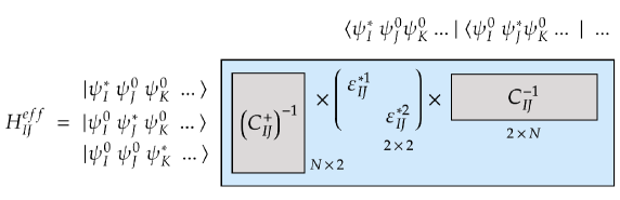
Figure 5: Schematic illustration of the construction of $H_{IJ}^{eff}$

When combine the ML-assisted coded computing with REM-TDDFT, one can first assign the possible excited monomers, then the excitable dimers can also be determined by considering the interacting monomers within a given distance, e.g. 4 Å. Basing on an specific excitable monomer, all the dimers that contains this monomer, and the all other monomers in the corresponding dimers can be treated as a group in coded computing. All sub-tasks (monomers and dimers) in a group can be encoded via the $A$, $B$ matrix basing on the Algorithm 1 and 2. After that, the coded and the no-coded sub-tasks can be assembled together, then the greedy algorithm can be used to optimize the scheduling basing on the predicted timing for the DFT/TDDFT calculations.

2.4 Implementation and workflow

The Fcst_sys package ⁴² is adapted for the augmented descriptor, so that the improved ML models can be employed for giving more accurate predictions. At the meantime, simple Matlab or Python script can be used to generate the coding and decoding matrices, which only involving the part/desired sub-tasks to be computed in the forthcoming distributed calculations. After encoding the desired sub-tasks, the encoded task-row, i.e. sub-tasks that was reflected as a row in the $B$ matrix, is treated as a single task. The predicted computational costs are the summation of individual sub-tasks in the task-row.

Once obtaining the predicted computational costs for all sub-tasks, including both no-coded and encoded ones, the planning algorithms like greedy can be employed to get the proposed SLB scheduling. The Python script is used to implement the scheduling, and supply the suggested scheduling for the distributed HPC calculations. The ParaEngine package, ²³ which is developed as a demonstrative engine for ML-assisted quantum chemical calculations, can be directly re-used as the coded quantum chemical engine with improved SLB scheduling. After all the calculations are done, the REM-TDDFT approach can be used to evaluate the excited states of the whole systems. Although the ground state can also the evaluated basing on the REM framework by simplifying the model space, the energy-based framework like MFCC, FMO approaches are more convenient.

The whole workflow is also illustrated in Fig.6 for a visual illustration.

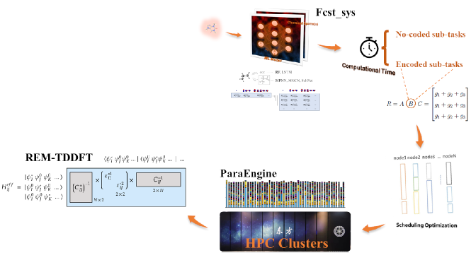
Figure 6: Workflow of the coded quantum chemical calculations with improved ML models.

3 RESULTS

3.1 Term-wise assessments

3.1.1 Improved ML models

The ”original”, ”aug-V”, and ”aug-M” ML models, which are proposed in sub-section 2.1, are evaluated using the same reference data obtained by B3LYP functional and several different basis sets, i.e. Pople’s 6-31g, 6-31g*, and 6-31+g*, separately. Additionally, evaluations in order of molecular weight (e.g. small: 1-200; middle: 200-400; large: $>$ 400), are also checked.

The results of bi-LSTM model with ”aug-V” treatment are showed in Fig.7(a) and Fig.7(b). It can be found that it changes little compared with its original form, whatever with different basis sets or with different system sizes. It is due to the augmented AOs information can not work well together with text-based models like bi-LSTM. Unlike the bi-LSTM model, obvious improvement can be observed for the graph-based models. The Fig.8(a) shows the results of MPNN models with ”aug-V and ”aug-M” amendments. It can be noticed that the MPNN model with ”aug-V” has better performance than that of original model, whatever for different basis sets (Fig.8(a)) or different system size (Fig.8(b)). The mean relative errors (MREs) show better convergence behaviour during the epoch iterations in this case. On the contrary, MPNN models with ”aug-M” does not change its curves much compared with that of its original model.The possible reason should be that the ”aug-M” combines new feature with its molecular features and then processes them for four levels, which makes the feature data lose its characteristics. On the other hand, it also means that the molecular feature data stream is mainly for the identification of molecular structure in calculation, rather than the identification of the AOs informations in a given chemical space.

\begin{overpic}[scale={0.50},bb=0 0 400 320]{Figs/LSTM_B3LYP_origin.eps} \put(63.0,54.0){original} \end{overpic}\begin{overpic}[scale={0.50},bb=0 0 400 310]{Figs/LSTM_B3LYP_bg.eps} \put(63.0,54.0){aug-V} \end{overpic}

(a) Different basis sets

\begin{overpic}[scale={0.50},bb=0 0 400 320]{Figs/LSTM_B3LYP_size_origin.eps} \put(68.0,54.0){original} \end{overpic}\begin{overpic}[scale={0.50},bb=0 0 400 310]{Figs/LSTM_B3LYP_size_bg.eps} \put(68.0,54.0){aug-V} \end{overpic}

(b) Different molecular weights

Figure 7: The calculated MRE in the training process with ”original” (upper) and ”aug-V” (bottom) bi-LSTM models, respectively.

\begin{overpic}[scale={0.50},bb=0 0 400 310]{Figs/MPNN_B3LYP_origin.eps} \put(50.0,64.0){original} \end{overpic}\begin{overpic}[scale={0.50},bb=0 0 400 310]{Figs/MPNN_B3LYP_bg.eps} \put(50.0,64.0){aug-V} \end{overpic}\begin{overpic}[scale={0.50},bb=0 0 400 310]{Figs/MPNN_B3LYP_ms.eps} \put(50.0,69.0){aug-M} \end{overpic}

(a) Different basis sets

\begin{overpic}[scale={0.50},bb=0 0 400 310]{Figs/MPNN_B3LYP_size_origin.eps} \put(59.0,64.0){original} \end{overpic}\begin{overpic}[scale={0.50},bb=0 0 400 310]{Figs/MPNN_B3LYP_size_bg.eps} \put(59.0,64.0){aug-V} \end{overpic}\begin{overpic}[scale={0.50},bb=0 0 400 310]{Figs/MPNN_B3LYP_size_ms.eps} \put(59.0,64.0){aug-M} \end{overpic}

(b) Different molecular weights

Figure 8: The calculated MRE in the training process with ”original” (left), ”aug-V” (middle), and ”aug-M” (right) MPNN models, separately.

3.1.2 Improved ML-assisted static load balancing

In the Fig.9 of Ref.23, we show that the ”ML-assisted SLB + DLB ” scheme can show the highest computational efficiency, and the SLB benefits the overall computational efficiency a lot in these distributed MFCC calculations of P38 protein. Once obtaining the improved ML models, the same P38 system (shown in Fig.9) can be used as the theoretical benchmark, in order to show the performance of improved models in scheduling. Because the existence of DLB may confuse the contributions that from SLB, only different SLB schemes are used in benchmarking.

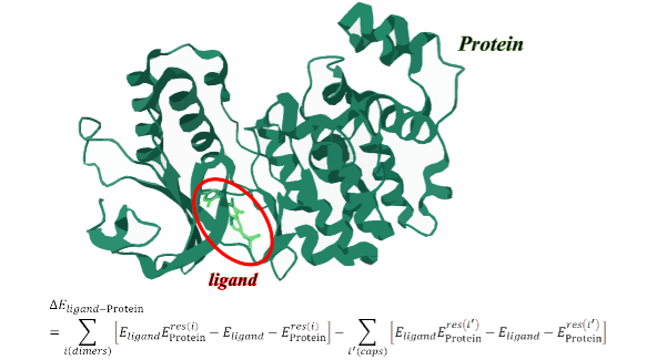
Figure 9: The P38 protein (PDB ID: 3FLY) is used when benchmarking various SLB schemes, and in checking the fault tolerance of coded MFCC calculations.

The default training suits in Fcst_sys ⁴² are used in training ML-models, and the ”aug-V” variants are also employed as the improved ML-models. These SLB schemes are denoted as SLB(LSTM, original, Fcst_sys), SLB(LSTM, aug-V, Fcst_sys), and SLB(MPNN, aug-V, Fcst_sys), separately. Moreover, the system-specific training suits, i.e. protein systems, are also used together with the same ”aug-V” variants, and denoted as SLB(LSTM, original, protein), SLB(LSTM, aug-V, protein), and SLB(MPNN, aug-V, protein), separately.

All the results of elapsed times using different SLB schemes by 50 distributed nodes are illustrated in Fig.10, and the analysis by the largest elapsed time and standard deviation are presented in Fig.11. It can be found that both the system-specific ML models and the ”aug-V” variants can improve the task distribution. The best combination is SLB(MPNN, aug-V, protein) scheme, in which the largest elapsed time in node is 4539 sec. with a small standard deviation.

\begin{overpic}[scale={0.3750},bb=10 0 1400 700]{Figs/ML-assisted_SLB.eps} \put(40.0,47.5){(A)} \put(40.0,30.5){(B)} \put(40.0,13.5){(C)} \put(50.0,47.5){(D)} \put(50.0,30.5){(E)} \put(50.0,13.5){(F)} \end{overpic}

Figure 10: The illustration of elapsed times for M06-2x/6-31G** snapshot of P38 protein using MFCC computational approach in the distributed case with 50 HPC nodes. Different scheduling schemes are employed, they are (A) SLB(LSTM, original, Fcst_sys), (B) SLB(LSTM, aug-V, Fcst_sys), (C) SLB(MPNN, aug-V, Fcst_sys), (D) SLB(LSTM, original, protein), (E) SLB(LSTM, aug-V, protein), (F) SLB(MPNN, aug-V, protein), separately. The (A), (D) are from Ref.23

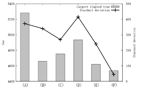
Figure 11: The largest elapsed time and the standard deviation for all the distributed HPC nodes when using different SLB schemes.

3.1.3 Coded quantum chemical calculations

The coded quantum chemical calculation is implemented with the MFCC and REM framework. The calculation of ligand-protein interaction of P38 protein (PDB ID: 3FLY), which is illustrated in Fig.9, is used as the example in checking the fault tolerance of coded calculation. It can be noticed that the binding/interaction energy can be treated as the ligand-dimer interaction minus the ligand-cap interaction, so that the no-redundant fragments in most calculations are the $E_{ligand}E^{res(i)}_{Protein}$, $E^{res(i)}_{Protein}$, $E_{ligand}E^{res(i^{\prime})}_{Protein}$, and $E^{res(i^{\prime})}_{Protein}$, separately. Notice that the $i$ and $i^{\prime}$ indexes the dimers and caps, respectively, and the no-redundant 4 fragments with same index of i/i’ can be treated as a minimum group unit for calculating protein-ligand interactions.

Basing on the idea of gradient coding, the task number $n$ can be set to 4, assuming the tolerable straggler node $s$ be 1, then the $B$ matrix listed in subsection 2.2.2 can be used as the encoding matrix. With the encoding-decoding process, there are 4 results can be obtained for the computation of a particular group unit. The decoded binding energies is compared with the reference energy that obtained in Ref.²³, and the few randomly selected results are presented in Table.1. For the fragments group with i/i’ as 0029, the encoding computations yield 4 identical results, indicating that all 4 computing nodes have correctly obtained the results. For the fragments group with i/i’ as 0062, calculations for one set of data on one node exceeded the threshold we had set, resulting in no returned result. However, from the remaining three computing nodes, the correct result can still be decoded.

Table 1: Checking the fault tolerance in the coded MFCC calculations for the binding energies in the randomly selected fragment groups.

Fragments group (i/i’)	Reference	Decoded binding energy
0029	$9.29399e^{-5}$	$9.29399e^{-5}$ $9.29399e^{-5}$ $9.29399e^{-5}$ $9.29399e^{-5}$
0062	$-6.86651e^{-5}$	$-6.86651e^{-5}$ (no result) (no result) (no result)

Once done the assessments of fault tolerance, the errors that may introduced by the encoding-decoding process are also checked. This time all the sampled fragments’ groups, as well as the derivations between results from encoding-decoding and these from reference, are shown in Fig.12. It can be notice that most derivations caused by encoding-decoding are less than 1.0e-10, and the largest derivation is in 1.0e-8 level. Actually, the 3.0e-8, 2.0e-8, 1.0e-8, and 1.0e-10 derivations for this specific coded fragments’ group may also reflect the very tiny convergence mismatch.

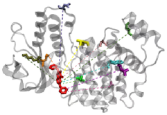
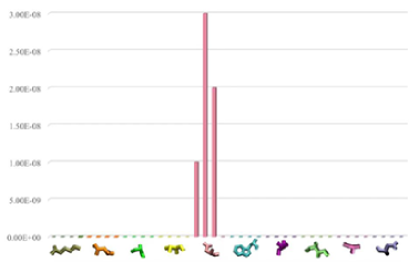
Figure 12: Derivations that may introduced by the encoding-decoding process are evaluated. Several fragment groups in coded calculating protein-ligand interactions are illustrated, and the derivations between results from encoding-decoding process and these from Ref.23 are also shown.

3.2 Applying in fragmented-based excited-state calculations

Once done the term-wise assessments for all components (improved ML-models, scheduling optimizing, coded computing, etc.) that may assist the practical quantum chemical calculations, we turns to the calculation of excited states with one or several excitable centers. The green fluorescent protein anion (GFPA) dye in water solvent, and the drug-water mixed molecular clusters are used as the benchmark systems, respectively.

3.2.1 Absorption spectra of GFPA in water solvent

Before the calculation of excited states of GFP solvent model, the reasonable structures should be obtained firstly using the molecular dynamic (MD) simulations. ⁷⁰ Herein, the generalized AMBER force field (GAFF) ⁷¹ for solute apart from water, which is described by the TIP3P model. ⁷² For the central dyes in question, we use the ANTECHAMBER program ⁷¹ to generate appropriate force field parameters, where the input structures are optimized in vacuum at the M06-2x/6-31G* level. The MD simulation is implemented by Amber using Langevin dynamics approach with a collision frequency of 1 $ps^{-1}$, then it start at 0K and target temperature of 300K and take several snapshot at this temperature.

Once the snapshot is obtained, the 100 waters that close to the central GFPA dye are picked up, and all the monomers within a inter-distance of 4Å are chosen as the dimers. If any dimers contain the central GFGA dye molecule, then both the dimers and the related monomers (waters and GFPA dye) are encoded during the excited states calculations using the TDDFT approach. Both the decoded and encoded sub-systems are handled together by the ParaEngine package for the convenience. ²³ After done the calculation, the REM-TDDFT approached can be invoked for obtaining the excited states for the whole systems. The result for a sampled snapshot is shown in Table.2. It can be notice that the adsorption is mainly located in the GFPA molecule in the solvent system, which is match the results of previous works. ⁷⁰

Nevertheless, we should mentioned that the encoding-decoding process can be applied to any observable parameters. In previous MFCC calculation of binding energy, the coded fragmented have the specific physical meanings, i.e. the binding energy from fragment group units. Actually, any related observables, e.g. excitation energies here, can be chosen as the markers that can be used in coded part. For example, the dimers that contains GFPA, specific waters in these dimers can be coded as a fragments group, upon which the $B$ matrix can be generated. The $B$ is a typical sparse matrix and can dot multiple with the position-specific non-redundant and redundant markers (i.e. excitation energies) to generate $B_{M}$, then the $A$ matrix can multiple with $B_{M}$ to get the $C_{M}$. If no abnormal occurs, all the vectors in $C_{M}$ are identical with each other as shown in subsection 2.2.2, it means no extra efforts needed to be introduced to correct the possible errors.

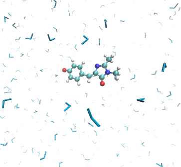
Figure 13: The illustration of GFPA in water solvent.

3.2.2 Low-lying excited states for clusters with several excitable centers

As the last calculations, the clusters with several excitable centers are used. The cluster models were packed by PackMol package ⁷³ using water and drug molecules from the DrugBank library. ⁷⁴ This system was also used in our previous work for the purpose of illustration of ”ML-assisted SLB + DLB” solvation effect calculations, and in this work the low-lying excited states that can beyond the ground state interactions are considered as well. There are 203 monomers including various drug molecules and waters. Due to this cluster is too large to get a reliable reference, a reduced cluster is picked up using some monomers from this original cluster. Both of the two molecular clusters (denoted as Cluster-1 and Cluster-2) are illustrated in Fig.14.

\begin{overpic}[scale={0.75},bb=00 0 200 200]{Figs/sol-ex-small1.eps} \put(24.0,75.0){Cluster-1} \end{overpic}

\begin{overpic}[scale={1.00},bb=00 0 200 200]{Figs/sol-ex-large1.eps} \put(-20.0,74.0){Cluster-2} \end{overpic}

Figure 14: The illustration of two molecular clusters with several excitable centers.

For the reduced molecular cluster, both the coded REM-TDDFT and the normal TDDFT calculations can be implemented by ParaEngine and Gaussian,⁷⁵ respectively. The calculated results are listed in Table.2. It can be noticed that the excitation energies for these two clusters are almost the same since is mainly stemmed from a specific monomer. However, the excitable monomers can be identified for more than this one specific monomer for both REM-TDDFT and TDDFT approaches in Cluster-1 systems. The wave functions of REM-TDDFT imply that more excitable monomers can be involved in the more complicated systems of Cluster-2.

Table 2: Calculated excitation energies of the lowest singlet excited states of the two cluster systems with REM-TDDFT and TDDFT approaches. The possible excited monomers are also listed for REM-TDDFT calculations with their coefficients are shown in brackets.

		REM-TDDFT				TDDFT
		eV	excitable monomers’ ID (weight)			eV
GFPA
$S_{1}$		3.104	1(1)			-
Cluster-1
$S_{1}$		2.518	12(0.76)    9(0.65)			2.509
Cluster-2
$S_{1}$		2.517	141(0.21)   138(0.39)  113(0.47)			-
			110(0.39)  65(0.39)  46(0.33)  6(0.39)

4 CONCLUSIONS

Basing on the recent work of ML-assisted scheduling optimization, we further propose 1) the improve ML models for the better predictions of computational loads; 2) the idea of coded computation to introduce fault tolerance during the distributed calculations; and 3) their applications together with REM framework for calculating the excited states. In the improved ML models, the descriptor for the basis sets is extended from a point to a vector (aug-V) or matrix (aug-M), and as such, obvious improvement for the accuracy in predictions can be observed. For example, about 50% reduction in MRE values when comparing the predicted results of MPNN(aug-V) to these of MPNN(original). For the coded computing, the gradient coding is introduced in order to provide fault tolerance during the distributed calculations, thus abnormal results caused by the convergence behavior or anomaly node can be detected or corrected. Both the improved ML models and the coded technique can be integrated in the ParaEngine package, in which the REM-TDDFT utility have already implemented for describing the excited states of large molecule and molecular clusters.

Illustrated benchmark calculations include P38 protein, and solvent model with one or several excitable centers. The results show that the both the computational efficiency and the capacity of fault tolerance can be improved. For instance, the SLB assignments can be at least improved by 10% $\sim$ 15% when the improved ML models are employed, and the coded computing can guarantee the abnormal results can be easily located with some of them can be corrected automatically. Additionally, their preliminary integration with MFCC and REM-TDDFT approaches show its potential usage in the ML-assisted automated fault-tolerant calculation for large systems.

Reaching the end, we should mention that the current implements are better work within HPC clusters. The cross-domain calculation is not implemented yet. Working on these direction is currently in progress in our laboratory. We hope the computational scheme can be finally evolved like Folding@Home⁷⁶ or Seti@Home,⁷⁷ so that more computational resources can be utilized to accelerate the related research.

ACKNOWLEDGMENTS

Y. Ma thank Prof. Haili Xiao for the en-lighting discussions of fault-tolerant. This work was supported by National Natural Science Foundation of China (No.22173114, 22333003 to Y. Ma and No.41971366, 42371476 to D. Guo), Strategic Priority Research Program of Chinese Academy of Sciences (XDB0500001), Youth Innovation Promotion Association of Chinese Academy of Sciences (No.2022168), Network and Information Foundation of Chinese Academy of Sciences (CAS$-$WX2021SF$-$0103$-$02), and Project of Computer Network Information Center, Chinese Academy of Science (CNIC20230201). K. Yuan also thank the support from College Students Innovative Practice Training Program of Chinese Academy of Sciences. Most of the computational experiments were implemented in the ”ORISE” and ”ERA” supercomputers, we are also highly appreciated the helps from the supporting team.

Data Availability Statement

The data that support the findings of this study are available from the corresponding author upon reasonable request.

References

- 1 Kitaura, K.; Ikeo, E.; Asada, T.; Nakano, T. and Uebayasi, M., Chem. Phys. Lett., 1999, 313(3-4), 701–706.
- 2 He, X. and Zhang, J. Z., J. Chem. Phys., 2005, 122(3), 031103.
- 3 He, X. and Zhang, J. Z., J. Chem. Phys., 2006, 124(18), 184703.
- 4 Fedorov, D. and Kitaura, K., The fragment molecular orbital method: practical applications to large molecular systems, CRC press, 2009.
- 5 Mayhall, N. J. and Raghavachari, K., J. Chem. Theory Comput., 2011, 7(5), 1336–1343.
- 6 Wang, X.; Liu, J.; Zhang, J. Z. and He, X., J. Phys. Chem. A, 2013, 117(32), 7149–7161.
- 7 Saebo, S. and Pulay, P., Annu. Rev. Phys. Chem., 1993, 44(1), 213–236.
- 8 Aquilante, F.; Bondo Pedersen, T.; Sanchez de Meras, A. and Koch, H., J. Chem. Phys., 2006, 125(17), 174101.
- 9 Li, W.; Piecuch, P.; Gour, J. R. and Li, S., J. Chem. Phys., 2009, 131(11), 114109.
- 10 Cole, D.; Skylaris, C.-K.; Rajendra, E.; Venkitaraman, A. and Payne, M., EPL, 2010, 91(3), 37004.
- 11 Wu, F.; Liu, W.; Zhang, Y. and Li, Z., J. Chem. Theory Comput., 2011, 7(11), 3643–3660.
- 12 Li, W., J. Chem. Phys., 2013, 138(1), 014106.
- 13 Riplinger, C.; Sandhoefer, B.; Hansen, A. and Neese, F., J. Chem. Phys., 2013, 139(13), 134101.
- 14 Li, Z.; Li, H.; Suo, B. and Liu, W., Accounts Chem. Res., 2014, 47(9), 2758–2767.
- 15 Li, W. and Li, S., J. Chem. Phys., 2005, 122(19), 194109.
- 16 Li, H.; Liu, W. and Suo, B., J. Chem. Phys., 2017, 146(10), 104104.
- 17 Ni, Z.; Li, W. and Li, S., J. Comput. Chem., 2019, 40(10), 1130–1140.
- 18 Kato, K.; Honma, T. and Fukuzawa, K., J. Mol. Graph. Model., 2020, 100, 107695.
- 19 Akisawa, K.; Hatada, R.; Okuwaki, K.; Mochizuki, Y.; Fukuzawa, K.; Komeiji, Y. and Tanaka, S., RSC Adv., 2021, 11(6), 3272–3279.
- 20 Akisawa, K.; Hatada, R.; Okuwaki, K.; Kitahara, S.; Tachino, Y.; Mochizuki, Y.; Komeiji, Y. and Tanaka, S., Jpn. J. Appl. Phys, 2021, 60(9), 090901.
- 21 Fukuzawa, K.; Kato, K.; Watanabe, C.; Kawashima, Y.; Handa, Y.; Yamamoto, A.; Watanabe, K.; Ohyama, T.; Kamisaka, K.; Takaya, D. and others, , J. Chem. Inf. Model., 2021, 61(9), 4594–4612.
- 22 Wannipurage, D.; Deb, I.; Abeysinghe, E.; Pamidighantam, S.; Marru, S.; Pierce, M. and Frank, A. T., arXiv preprint arXiv:2201.12237, 2022.
- 23 Ma, Y.; Li, Z.; Chen, X.; Ding, B.; Li, N.; Lu, T.; Zhang, B.; Suo, B. and Jin, Z., Journal of Computational Chemistry, 2023, 44(12), 1174–1188.
- 24 Li, Z.; Li, H.; Yu, K. and Luo, H.-B., National Science Review, 2021, 8(12), nwab105.
- 25 Chen, X.; Liu, M. and Gao, J., J. Chem. Theory Comput., 2022, 18(3), 1297–1313.
- 26 Green, M. L.; Choi, C.; Hattrick-Simpers, J.; Joshi, A.; Takeuchi, I.; Barron, S.; Campo, E.; Chiang, T.; Empedocles, S.; Gregoire, J. and others, , Applied Physics Reviews, 2017, 4(1).
- 27 de Pablo, J. J.; Jackson, N. E.; Webb, M. A.; Chen, L.-Q.; Moore, J. E.; Morgan, D.; Jacobs, R.; Pollock, T.; Schlom, D. G.; Toberer, E. S. and others, , npj Computational Materials, 2019, 5(1), 41.
- 28 Liu, Y.; Niu, C.; Wang, Z.; Gan, Y.; Zhu, Y.; Sun, S. and Shen, T., Journal of Materials Science & Technology, 2020, 57, 113–122.
- 29 Suh, C.; Fare, C.; Warren, J. A. and Pyzer-Knapp, E. O., Annual Review of Materials Research, 2020, 50, 1–25.
- 30 Pyzer-Knapp, E. O.; Pitera, J. W.; Staar, P. W.; Takeda, S.; Laino, T.; Sanders, D. P.; Sexton, J.; Smith, J. R. and Curioni, A., npj Computational Materials, 2022, 8(1), 84.
- 31 Fujita, T. and Mochizuki, Y., J. Phys. Chem. A, 2018, 122(15), 3886–3898.
- 32 Ni, Z.; Wang, Y.; Li, W.; Pulay, P. and Li, S., J. Chem. Theory Comput., 2019, 15(6), 3623–3634.
- 33 Abraham, V. and Mayhall, N. J., J. Chem. Theory Comput., 2020, 16(10), 6098–6113.
- 34 Wang, K.; Xie, Z.; Luo, Z. and Ma, H., J. Phys. Chem. Lett., 2022, 13(2), 462–470.
- 35 Alexeev, Y.; Mahajan, A.; Leyffer, S.; Fletcher, G. and Fedorov, D. G. In SC’12: Proceedings of the International Conference on High Performance Computing, Networking, Storage and Analysis, pages 1–13. IEEE, 2012.
- 36 Gaussier, E.; Glesser, D.; Reis, V. and Trystram, D. In Proceedings of the International Conference for High Performance Computing, Networking, Storage and Analysis, pages 1–10, 2015.
- 37 Helmy, T.; Al-Azani, S. and Bin-Obaidellah, O. In 2015 3rd International Conference on Artificial Intelligence, Modelling and Simulation (AIMS), pages 3–8. IEEE, 2015.
- 38 Shulga, D.; Kapustin, A.; Kozlov, A.; Kozyrev, A. and Rovnyagin, M. In 2016 IEEE NW Russia Young Researchers in Electrical and Electronic Engineering Conference (EIConRusNW), pages 345–348. IEEE, 2016.
- 39 Fedorov, D. G. and Pham, B. Q., The Journal of Chemical Physics, 2023, 158(16).
- 40 Heinen, S.; Schwilk, M.; von Rudorff, G. F. and von Lilienfeld, O. A., Machine Learning: Science and Technology, 2020, 1(2), 025002.
- 41 Wei Jianwen, Wang Liuzhen, W. Y. e. a. In Proceedings of the 2021 National High Performance Computing Annual Conference, pages 519–527. Zhuhai: China Computer Society, 2021.
- 42 Ma, S.; Ma, Y.; Zhang, B.; Tian, Y. and Jin, Z., ACS omega, 2021, 6(3), 2001–2024.
- 43 Yadwadkar, N. J.; Hariharan, B.; Gonzalez, J. E.; R, and y Katz, , Journal of Machine Learning Research, 2016, 17(106), 1–37.
- 44 Tandon, R.; Lei, Q.; Dimakis, A. G. and Karampatziakis, N. In Precup, D. and Teh, Y. W., Eds., Proceedings of the 34th International Conference on Machine Learning, Vol. 70 of Proceedings of Machine Learning Research, pages 3368–3376. PMLR, 2017.
- 45 Li, S.; Maddah-ali, M. A.; Yu, Q. and Avestimehr, A. S., IEEE Transactions on Information Theory, 2016, 64, 109–128.
- 46 Attia, M. A. and Tandon, R., IEEE Transactions on Information Theory, 2019, 65(11), 7325–7349.
- 47 Kianidehkordi, S.; Ferdinand, N. S. and Draper, S. C., IEEE Transactions on Information Theory, 2021, 67, 726–754.
- 48 Wang, J.; Cao, C.; Wang, J.; Lu, K.; Jukan, A. and Zhao, W., IEEE Transactions on Cloud Computing, 2022, 10(4), 2817–2833.
- 49 Chen, Z.; Fagg, G. E.; Gabriel, E.; Langou, J.; Angskun, T.; Bosilca, G. and Dongarra, J. In Proceedings of the tenth ACM SIGPLAN symposium on Principles and practice of parallel programming, pages 213–223, 2005.
- 50 Fahim, M. and Cadambe, V. R., IEEE Transactions on Information Theory, 2021, 67(5), 2758–2785.
- 51 Li, C.; Zhang, Y. and Tan, C. W., IEEE Transactions on Communications, 2023.
- 52 https://en.wikipedia.org/wiki/Hamming_code, (accessed date Oct. 23, 2023).
- 53 Schütt, K. T.; Gastegger, M.; Tkatchenko, A.; Müller, K.-R. and Maurer, R. J., Nature communications, 2019, 10(1), 5024.
- 54 Gastegger, M.; McSloy, A.; Luya, M.; Schütt, K. T. and Maurer, R. J., The Journal of Chemical Physics, 2020, 153(4).
- 55 Unke, O.; Bogojeski, M.; Gastegger, M.; Geiger, M.; Smidt, T. and Müller, K.-R., Advances in Neural Information Processing Systems, 2021, 34, 14434–14447.
- 56 Li, H.; Wang, Z.; Zou, N.; Ye, M.; Xu, R.; Gong, X.; Duan, W. and Xu, Y., Nature Computational Science, 2022, 2(6), 367–377.
- 57 Gong, X.; Li, H.; Zou, N.; Xu, R.; Duan, W. and Xu, Y., Nature Communications, 2023, 14(1), 2848.
- 58 Li, H.; Tang, Z.; Gong, X.; Zou, N.; Duan, W. and Xu, Y., Nature Computational Science, 2023, 3(4), 321–327.
- 59 https://en.wikipedia.org/wiki/Linear_combination_of_atomic_orbitals, (accessed date Oct. 24, 2023).
- 60 Gilmer, J.; Schoenholz, S. S.; Riley, P. F.; Vinyals, O. and Dahl, G. E. In International Conference on Machine Learning, pages 1263–1272. PMLR, 2017.
- 61 Lu, C.; Liu, Q.; Wang, C.; Huang, Z.; Lin, P. and He, L. In Proceedings of the AAAI Conference on Artificial Intelligence, Vol. 33, pages 1052–1060, 2019.
- 62 Graves, A.; Fernández, S. and Schmidhuber, J. In International conference on artificial neural networks, pages 799–804. Springer, 2005.
- 63 Reisizadeh, A.; Prakash, S.; Pedarsani, R. and Avestimehr, A. S., IEEE Transactions on Information Theory, 2019, 65(7), 4227–4242.
- 64 Li, S.; Avestimehr, S. and others, , Foundations and Trends® in Communications and Information Theory, 2020, 17(1), 1–148.
- 65 Ma, Y.; Liu, Y. and Ma, H., The Journal of Chemical Physics, 2012, 136(2).
- 66 Ma, Y. and Ma, H., The Journal of Physical Chemistry A, 2013, 117(17), 3655–3665.
- 67 Zhang, H.; Malrieu, J.-P.; Ma, H. and Ma, J., 33(1), 34–43.
- 68 Liu, Y.-h.; Wang, K. and Ma, H.-b., 34(6).
- 69 Wang, K.; Xie, Z.; Luo, Z. and Ma, H., 13(2), 462–470.
- 70 Zuehlsdorff, T. J. and Isborn, C. M., The Journal of Chemical Physics, 2018, 148(2).
- 71 Wang, J.; Wolf, R. M.; Caldwell, J. W.; Kollman, P. A. and Case, D. A., Journal of computational chemistry, 2004, 25(9), 1157–1174.
- 72 Jorgensen, W. L.; Chandrasekhar, J.; Madura, J. D.; Impey, R. W. and Klein, M. L., The Journal of chemical physics, 1983, 79(2), 926–935.
- 73 Martínez, L.; Andrade, R.; Birgin, E. G. and Martínez, J. M., J. Comput. Chem., 2009, 30(13), 2157–2164.
- 74 Wishart, D. S.; Feunang, Y. D.; Guo, A. C.; Lo, E. J.; Marcu, A.; Grant, J. R.; Sajed, T.; Johnson, D.; Li, C.; Sayeeda, Z. and others, , Nucleic Acids Res., 2018, 46(D1), D1074–D1082.
- 75 Frisch, M. J.; Trucks, G. W.; Schlegel, H. B.; Scuseria, G. E.; Robb, M. A.; Cheeseman, J. R.; Scalmani, G.; Barone, V.; Mennucci, B.; Petersson, G. A.; Nakatsuji, H.; Caricato, M.; Li, X.; Hratchian, H. P.; Izmaylov, A. F.; Bloino, J.; Zheng, G.; Sonnenberg, J. L.; Hada, M.; Ehara, M.; Toyota, K.; Fukuda, R.; Hasegawa, J.; Ishida, M.; Nakajima, T.; Honda, Y.; Kitao, O.; Nakai, H.; Vreven, T.; Montgomery, Jr., J. A.; Peralta, J. E.; Ogliaro, F.; Bearpark, M.; Heyd, J. J.; Brothers, E.; Kudin, K. N.; Staroverov, V. N.; Kobayashi, R.; Normand, J.; Raghavachari, K.; Rendell, A.; Burant, J. C.; Iyengar, S. S.; Tomasi, J.; Cossi, M.; Rega, N.; Millam, J. M.; Klene, M.; Knox, J. E.; Cross, J. B.; Bakken, V.; Adamo, C.; Jaramillo, J.; Gomperts, R.; Stratmann, R. E.; Yazyev, O.; Austin, A. J.; Cammi, R.; Pomelli, C.; Ochterski, J. W.; Martin, R. L.; Morokuma, K.; Zakrzewski, V. G.; Voth, G. A.; Salvador, P.; Dannenberg, J. J.; Dapprich, S.; Daniels, A. D.; Farkas, Ö.; Foresman, J. B.; Ortiz, J. V.; Cioslowski, J. and Fox, D. J., Gaussian09 Revision D.01, 2009.
- 76 Voelz, V. A.; Pande, V. S. and Bowman, G. R., Biophysical Journal, 2023.
- 77 Anderson, D. P.; Cobb, J.; Korpela, E.; Lebofsky, M. and Werthimer, D., Communications of the ACM, 2002, 45(11), 56–61.