Incorporating Riemannian Geometric Features for Learning Coefficient of Pressure Distributions on Airplane Wings

Abstract

The aerodynamic coefficients of aircrafts are significantly impacted by its geometry, especially when the angle of attack (AoA) is large. In the field of aerodynamics, traditional polynomial-based parameterization uses as few parameters as possible to describe the geometry of an airfoil. However, because the 3D geometry of a wing is more complicated than the 2D airfoil, polynomial-based parameterizations have difficulty in accurately representing the entire shape of a wing in 3D space. Existing deep learning-based methods can extract massive latent neural representations for the shape of 2D airfoils or 2D slices of wings. Recent studies highlight that directly taking geometric features as inputs to the neural networks can improve the accuracy of predicted aerodynamic coefficients. Motivated by geometry theory, we propose to incorporate Riemannian geometric features for learning Coefficient of Pressure ($C_{P}$) distributions on wing surfaces. Our method calculates geometric features (Riemannian metric, connection, and curvature) and further inputs the geometric features, coordinates and flight conditions into a deep learning model to predict the $C_{P}$ distribution. Experimental results show that our method, compared to state-of-the-art Deep Attention Network (DAN), reduces the predicted mean square error (MSE) of $C_{P}$ by an average of 8.41% for the DLR-F11 aircraft test set.

Riemannian space, Geometric feature, Riemannian manifold, Deep learning.

1 INTRODUCTION

The aerodynamic coefficients of an aircraft are significantly influenced by its geometric shape, especially when the angle of attack (AoA) is large. The prevalent approach for aircraft geometry description is polynomial-based parameterization, such as Parametric Section (PARSEC) [1], Class Function/Shape Function Transformation (CST) [2], B-spline curves/surfaces [3], and Bézier curves/surfaces [4], etc. These methods typically utilize a minimal number of essential parameters to represent the geometric structure of an aircraft [5]. For example, a 4th-order CST parameterization method was used to extract 8 essential parameters as features to represent the shape of NACA0012 airfoil [6]. However, using only a small number of parameters as features makes it difficult to represent the entire geometry of wings in 3D space [7]. Instead, massive feature extraction as indicated in studies like [8, 9, 10] may provide a suitable idea for the representation of wings in 3D space.

In recent years, it has been demonstrated that deep learning, as a data-driven approach, can extract massive latent neural representations as features for geometries of objects in 3D space [11, 12, 13]. In the field of aerodynamics, there is a growing trend in utilizing deep learning-based methods to extract neural representations for aircraft shapes. Yang et al. applied a Variational Autoencoder (VAE) to optimize the shape of the GA(W)-1 airfoil according to the distribution of its Coefficient of Pressure ($C_{P}$) [14]. Du et al. combined B-spline curves with a Generative Adversarial Network (GAN) to develop BSpline-GAN, enabling the generation of a wide variety of airfoils [15]. Zahn et al. utilized a Convolutional Neural Network (CNN)-based Autoencoder to extract features from a 3D wing and predict its buffet pressure loads [16]. In the above studies, the shape of an aircraft is typically organized in the form of images or 2D slices [17]. Recent studies indicate that taking massive geometric features extracted from 2D airfoil slices as the inputs of deep learning models can improve the prediction accuracy of Coefficient of Lift ($C_{L}$), Coefficient of Drag ($C_{D}$) and $C_{P}$ [18, 19, 20], which may provide a way to predict $C_{P}$ distributions on wing surfaces in 3D space.

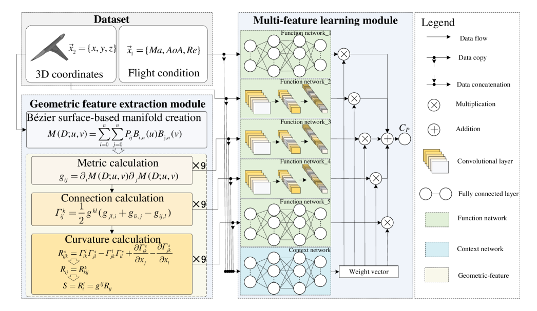
Motivated by both differential geometry and deep learning, we propose a learning method that incorporates Riemannian geometric features for predicting $C_{P}$ distributions on wing surfaces in 3D space . This method comprises two distinct submodules: a geometric feature extraction module and a multi-feature learning module. In the geometric feature extraction module, a set of self-intersection-free Bézier surfaces is used to approximate a wing surface in 3D space to construct a piecewise smooth Riemannian manifold. Subsequently, three geometric features (Riemannian metric, connection, and curvature) at a specific point as well as its 8 neighbors are calculated from the Riemannian manifold to represent the geometry of the wing. Within the multi-feature learning module, flight conditions, coordinates, and geometric features of the wing are incorporated to predict $C_{P}$.

In summary, the contributions of our work are

1. We use a set of self-intersection-free Bézier surface approximating the surface of a wing in 3D space to describe its geometry;

2. We demonstrate that geometric features (Riemannian metric, connection and curvature) can be used to represent the geometry of wings in 3D space;

3. We incorporate flight conditions, coordinates and geometric features of wings in 3D space into a deep learning model to predict $C_{P}$ distributions on the wing surface, which outperforms existing methods.

The remainder of this paper is organized as follows. Section 2 provides an overview of learning methods for aerodynamic coefficient predictions based on two different aircraft shape representations. In Section 3, we introduce the construction of the piecewise smooth manifold for a wing in 3D space, and the calculation of its geometric features. Furthermore, we introduce how to incorporate geometric features, coordinates and flight conditions into a deep learning model to predict $C_{P}$ distributions on the wing surface. In Section 4, a public DLR-F11 aircraft dataset [21] is used to validate the effectiveness of our method. The conclusions of our work are presented in Section 5.

2 RELATED WORKS

In this section, we discuss the state-of-the-arts in the field of aircraft shape representations for aerodynamic coefficient predictions. Specifically, we focus on aerodynamic coefficient predictions based on aircraft image (slice) shape representations and aerodynamic coefficient predictions based on aircraft manifold shape representations.

2.1 Aerodynamic coefficient predictions based on aircraft image (slice) shape representations

This method commonly organize the shape of aircrafts into multiple images or 2D slices and input them into deep learning models to obtain massive latent neural representations for aircraft shapes [22, 23, 24]. Zuo [25] et al. proposed a Deep Attention Network (DAN) model to extract neural representations from airfoil dataset provided by University of Illinois Urbana-Champaign (UIUC) [26]. The core concept of DAN is to generate latent neural representations from airfoil images by utilizing a Vision Transformer (VIT) [27], and then taking the neural representations and flight conditions of airfoils as inputs of a Multi-Layer Perceptron (MLP) submodule to predict the $C_{P}$ distribution on airfoil curves. Li et al. used a Deep Convolution neural network (DCNN)-based geometric filtering model to identify abnormalities in airfoils generated by Wasserstein GAN (WGAN), and further to predicted the $C_{P}$ distributions for normal airfoils. Notably, all input airfoils were structured as images, and the abnormalities detection and the $C_{P}$ prediction are achieved through the classification and regression of DCNN [24]. Qu et al. divided a wing in 3D space into multiple 2D slices and used a DCNN to predict $C_{P}$ distribution for each slice [28]. Similar studies can be found in [29, 30, 31].

The above studies can predict $C_{P}$ distributions for 2D airfoils or slices. However, the aerodynamic coefficient predictions based on shape representations of aircraft manifolds, as discussed below, has been shown to further improve the prediction accuracy.

Figure 1: The structure of our proposed method. The geometric features (Riemannian metric, connection, and curvature) are calculated from an aircraft wing in 3D space by geometric feature extraction submodule. Then the flight conditions, coordinates and geometric features are taken as inputs to a multi-feature submodule to predict the $C_{P}$ distribution on wing surface.

2.2 Aerodynamic coefficient predictions based on aircraft manifold shape representations

In this method, the curved shape of an aircraft is typically mapped into a low dimensional space [32, 33], and the shape representations of aircraft are expressed by calculating geometric features based on parameters defined in the low dimensional space.

Wang et al. used cubic splines to establish a mapping between the original 2D Cartesian coordinates of UIUC airfoils and 1D curvilinear coordinates [34]. Deng et al. utilized a univalent transformation to convert the geometrical information of airfoil mesh from 2D Cartesian coordinates to curvilinear coordinates [19]. The studies mentioned above utilize curvilinear coordinates as features to represent airfoil geometry. However, fundamentally, this approach is not significantly different from using Cartesian coordinates to represent geometries, because there is no further geometric feature extractions. Xiang et al. used a set of Bézier curves to transform UIUC airfoils represented by 2D coordinates into a 1D manifold, and further calculated the Riemannian metric as a geometric feature to represent the geometry of airfoils, which results in a significant reduction in the predicted mean square error (MSE) for $C_{D}$, compared to using images (slices) as inputs [18].

The above studies were carried out on 2D airfoils, and to the best of our knowledge, there has been no studies on constructing manifolds for wing surfaces in 3D space and extracting further geometric features for them.

In summary, compared with aerodynamic coefficient predictions based on aircraft image (slice) shape representations, aerodynamic coefficient predictions based on aircraft manifold shape representations can further reduce the prediction errors of aerodynamic coefficients. However, in aerodynamic coefficient predictions based on aircraft manifold shape representations, existing studies focused on shape representations for 2D airfoils, and the challenge of this method is how to extract massive geometric features for wings in 3D space.

3 METHODOLOGY

3.1 Overview

As shown in Fig.1, our method consists of two submodules: a geometric feature extraction module and a multi-feature learning module. In the geometric feature extraction module, a set of self-intersection-free Bézier surfaces is used to approximate a wing in 3D space to form a piecewise smooth manifold, and then Riemannian metric $g_{ij}$, connection $\mit\Gamma_{ij}^{k}$ and curvature $S$ are calculated as three geometric features to represent the geometry of the wing. Because the relation between wing geometry and its $C_{P}$ distribution is highly nonlinear, and the $C_{P}$ value at a specific point $P_{ab}$ ($a$ and $b$ are the subscripts of control point matrix) is related to a neighborhood around $P_{ab}$, the geometric features of 9 points ($P_{ab}$ and its 8 neighbors) are given as inputs. In the multi-feature learning module, the flight condition $\vec{\mathbf{x}}_{1}$, the coordinate points $\vec{\mathbf{x}}_{2}$ and three geometric features ($g_{ij}$, $\mit\Gamma_{ij}^{k}$ and $S$ related to 9 points) are taken as inputs to function network_1 $\sim$ function network_5, respectively. The context network takes $[\vec{\mathbf{x}}_{1},\vec{\mathbf{x}}_{2},g_{ij},\mit\Gamma_{ij}^{k},S]$ as input. The output is $C_{P}$. The multi-feature learning structure [18, 35, 36] has been shown to be more accurate in predicting aerodynamic coefficients compared to a MLP, which explains why we use the multi-feature learning structure to predict $C_{P}$. We will further test the advantages of the multi-feature learning structure in the experiments.

3.2 The geometric feature extraction module

3.2.1 Construction of the wing manifold

In this section, we use a set of self-intersection-free [18] Bézier surfaces that approximates a wing in 3D space to form a piecewise smooth manifold (we call each part of the piecewise smooth manifold a segment).

To simplify the description, we focus on a specific segment. Consider a set of wing control points in 3D space:

$$D=\begin{bmatrix}P_{00}&P_{01}&\cdots&P_{0n}\\ P_{10}&P_{ab}&\cdots&P_{1n}\\ \vdots&\vdots&\ddots&\vdots\\ P_{m0}&P_{m1}&\cdots&P_{mn}\end{bmatrix}$$

where $P_{ab}=(x_{ab},y_{ab},z_{ab})$, $a=1,2,\cdots,m$ and $b=1,2,\cdots,n$. A Bézier surface can be built:

$$\begin{cases}F(u,v)=\sum_{a=0}^{m}\sum_{b=0}^{n}P_{ab}B_{a,m}(u)B_{b,n}(v)\\ B_{a,m}(u)=\frac{m!}{a!(m-a)!}u^{a}(1-u)^{m-a}\\ B_{b,n}(v)=\frac{n!}{b!(n-b)!}v^{b}(1-v)^{n-b}\end{cases}$$ (1)

where $F(u,v)$ is a Bézier surface function. Since a Bézier surface is formed by the interweaving of two Bézier curves, the Bézier surface function $F(u,v)$ is determined by two parameters $u$ and $v$, $u,v\in[0,1]$. The variables $m$ and $n$ are the degrees of the two Bézier curves, and $B_{a,m}(u)$ and $B_{b,n}(v)$ are two coefficients of the Bézier surface.

Formula (1) can be written as

$$F(u,v)=\vec{B}_{u}\cdot\left[\begin{array}[]{cccc}P_{00}&P_{01}&\cdots&P_{0n}\\ P_{10}&P_{11}&\cdots&P_{1n}\\ \vdots&\vdots&\ddots&\vdots\\ P_{m0}&P_{m1}&\cdots&P_{mn}\end{array}\right]\cdot\vec{B}_{v}$$ (2)

where $\vec{B}_{u}=(B_{0,m}(u),B_{1,m}(u),\cdots,B_{m,m}(u))$ and ${\vec{B}_{v}}^{\top}=(B_{0,n}(v),B_{1,n}(v),\cdots,B_{n,n}(v))$.

The Jacobian matrix of $F(u,v)$ is:

$$\large J_{F}=d(F(u,v))=\begin{bmatrix}\frac{\partial F_{x}}{\partial u}&\frac{\partial F_{x}}{\partial v}\\[6.0pt] \frac{\partial F_{y}}{\partial u}&\frac{\partial F_{y}}{\partial u}\\[6.0pt] \frac{\partial F_{z}}{\partial u}&\frac{\partial F_{z}}{\partial u}\end{bmatrix}.$$ (3)

The rank of $J_{F}$ is determined by the linearity of two vectors $(\frac{\partial F_{x}}{\partial u},\frac{\partial F_{y}}{\partial u},\frac{\partial F_{z}}{\partial u})$ and $(\frac{\partial F_{x}}{\partial v},\frac{\partial F_{y}}{\partial v},\frac{\partial F_{z}}{\partial v})$. When the two vectors are linearly independent, the rank of $J_{F}$ is 2. In this case, $F(u,v)$ is an injection [37, 38] (i.e., $F(u,v)$ is a smooth immersion [39, 38]). If the function $F(u,v)$ has no self-intersections, then $F(u,v)$ is a smooth embedding in $\mathbb{R}^{3}$ [38]. Multiple smooth embeddings are concatenated together to form a piecewise smooth manifold which is denoted as $\mathcal{M}$.

3.2.2 Calculation of geometric features

(1) Riemannian metric: A Riemannian metric $g_{ij}$ defined at an arbitrary point $p_{ab}\in\mathcal{M}$, is a smooth covariant 2-tensor field representing an inner product on the tangent space of $\mathcal{M}$ (denoted as $T_{p_{ab}}\mathcal{M}$). The function $F(u,v)$ maps a parameter combination $\left\{x_{1}=u,x_{2}=v\right\}$ in $\mathbb{R}^{2}$ to a point $P_{ab}\in\mathcal{M}$, i.e., $F(x_{1},x_{2})=P_{ab}$. Therefore, the Riemannian metric can be calculated as

$$g_{ij}= \langle\frac{\partial}{\partial x_{i}}F(u,v),\frac{\partial}{\partial x_{j}}F(u,v)\rangle$$ (4)

$$= \partial_{i}F(u,v)\partial_{j}F(u,v)$$

where $i,j=\left\{1,2\right\}$, and $\partial_{i}=\frac{\partial}{\partial x_{i}}$ denotes the direction of the partial derivative.

(2) Riemannian connection: On a Riemannian manifold $(\mathcal{M},g)$, there exists a unique connection $\nabla$ which satisfies [40]

1. $\nabla$ is compatible with the metric $g$;

2. torsion-free.

This connection is called the Levi-Civita connection [41, 42], and we use this connection in this paper.

The connection $\nabla_{X}Y$ is a derivative of a vector field $Y$ on $(\mathcal{M},g)$ in the direction of another vector field $X$, which is also known as the covariant derivative of $Y$ along $X$ [43]. Suppose that $X=v^{i}(x)\partial_{x^{i}}$ and $Y=w^{i}(x)\partial_{x^{i}}$ are two vector fields on $(\mathcal{M},g)$, then

$$\nabla_{X}Y=\left(X\left(w^{k}\right)+v^{i}w^{j}\Gamma^{k}_{ij}\right)\partial_{x^{k}}.$$ (5)

The connection coefficient $\Gamma^{k}_{ij}$, the Christoffel symbols [44], can be written as

$$\Gamma^{k}_{ij} =\frac{1}{2}g^{kl}\left(\partial_{x^{i}}g_{jl}+\partial_{x^{j}}g_{li}-\partial_{x^{l}}g_{ij}\right)$$ (6)

$$=\frac{1}{2}g^{kl}\left(g_{jl,i}+g_{li,j}-g_{ij,l}\right)$$

where $g^{kl}$ denotes the inverse matrix of $g_{kl}$, and $i,j,k,l=\left\{1,2\right\}$. In Formula (6), we use the Einstein summation conventions [45]. Details of the connection formulas can be found in [40].

(3) Curvature: Curvature is a measure of whether a Riemannian manifold $(\mathcal{M},g)$ is flat or curved. Curvature is defined in the form of covariant derivative by evaluation on three vector fields $X$, $Y$, $Z$:

$$R(X,Y)Z=\nabla_{X}\nabla_{Y}Z-\nabla_{Y}\nabla_{X}Z-\nabla_{[X,Y]}Z$$ (7)

where Lie bracket $[X,Y]$ [46] denotes the anticommutativity of $X$ and $Y$. Suppose that $X=v^{i}(x)\partial_{x^{i}}$, $Y=w^{i}(x)\partial_{x^{i}}$ and $Z=u^{i}(x)\partial_{x^{i}}$, the curvature $R(X,Y)Z$ can also be written as

$$R(X,Y)Z =R(v^{i}(x)\partial_{x^{i}},w^{j}(x)\partial_{x^{j}})u^{k}(x)\partial_{x^{k}}$$ (8)

$$=v^{i}(x)w^{j}(x)u^{k}(x)R(\partial_{x^{i}},\partial_{x^{j}})\partial_{x^{k}}$$

$$=v^{i}(x)w^{j}(x)u^{k}(x)R_{ijk}^{s}\partial_{x^{s}}.$$

Associated with (7) and (8), we get the curvature coefficient $R_{ijk}^{s}$:

$$R_{ijk}^{s}=\left(\Gamma_{ik}^{l}\Gamma_{jl}^{s}-\Gamma_{jk}^{l}\Gamma_{il}^{s}\right)+\frac{\partial\Gamma_{ik}^{s}}{\partial x_{j}}-\frac{\partial\Gamma_{jk}^{s}}{\partial x_{i}}$$ (9)

where $i,j,k,s=\left\{1,2\right\}$. The Ricci curvature and scalar curvature [47] are used to simplify the 4-tensor $R_{ijk}^{s}$:

$$R_{ij}=R_{kij}^{k}$$ (10)

$$S=R_{i}^{i}=g^{ij}R_{ij}$$ (11)

where $R_{ij}$ denotes Ricci curvature and $S$ denotes scalar curvature. Details of curvature, Ricci curvature and scalar curvature can be found in [37].

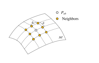
(4) Geometric features for 9 points: We take geometric features of $P_{ab}$ and its 8 neighbors as inputs for the multi-feature learning module. Fig. 2 shows how to select the 8 neighbors for $P_{ab}$. It is worth noting that all points should be on $\mathcal{M}$, and the distance $d$ between points is a hyperparameter. If the value of $d$ is relatively small, the geometric features of neighbors and $P_{ab}$ are relatively similar.

Figure 2: The selection of neighbors.

3.3 The multi-feature learning module

In this section, we introduce the multi-feature learning submodule from two aspects: The structure and the training method.

3.3.1 Structure

As shown in Fig.1, the module consists of five function networks and a context network. The function network_1 learns a nonlinear mapping between flight conditions $\vec{\mathbf{x}}_{1}$ and $C_{P}$, the function network_2 learns a nonlinear mapping between coordinate point $\vec{\mathbf{x}}_{2}$ on a wing surface and $C_{P}$, the function network_3 learns a nonlinear mapping between Riemannian metric $g_{ij}$ at coordinate point $\vec{\mathbf{x}}_{2}$ and $C_{P}$, the function network_4 learns a nonlinear mapping between connection $\mit\Gamma_{ij}^{k}$ at coordinate point $\vec{\mathbf{x}}_{2}$ and $C_{P}$, the function network_5 learns a nonlinear mapping between scalar curvature $S$ at coordinate point $\vec{\mathbf{x}}_{2}$ and $C_{P}$. The context network learns the fusion strategy (i.e., weight vector) for outputs generated by the five function networks.

The input of this module can be expressed as

$$\begin{cases}\vec{\mathbf{x}}_{1}=[Ma,AoA,Re]\\ \vec{\mathbf{x}}_{2}=\left\{x,y,z\right\}\\ \vec{\mathbf{x}}_{3}=\left\{g_{ij}\right\}\\ \vec{\mathbf{x}}_{4}=\left\{\mit\Gamma_{ij}^{k}\right\}\\ \vec{\mathbf{x}}_{5}=\left\{S\right\}\end{cases}$$ (12)

where $Ma$ denotes the incoming Mach number, $AoA$ denotes the Angle of Attack, $Re$ denotes the Reynolds number.

The output of this module is:

$$\hat{C}_{P}=\sum_{z=1}^{5}f_{z\alpha}(\vec{\mathbf{x}}_{z})\times c_{\left(z-1\right)K+\alpha}(\vec{\bm{\xi}})$$ (13)

where $\hat{C}_{P}$ denotes the predicted value, $f_{z\alpha}(\vec{\mathbf{x}}_{z})$ denotes the $\alpha$th component of the output vector from function network_$z$, $K$ denotes the number of output nodes in function networks, $c_{\alpha}(\vec{\bm{\xi}})$ denotes the $\alpha$th component of the output vector from the context network, and $\vec{\bm{\xi}}=[\vec{\mathbf{x}}_{1},\vec{\mathbf{x}}_{2},\vec{\mathbf{x}}_{3},\vec{\mathbf{x}}_{4},\vec{\mathbf{x}}_{5}]$ denotes the concatenation of $\vec{\mathbf{x}}_{1}\sim\vec{\mathbf{x}}_{5}$.

3.3.2 Training method

The loss function of the multi-feature learning module is:

$$L=\frac{1}{M}\sum_{\beta=1}^{M}\left(C_{P_{tr}}^{\beta}-\hat{C}_{P}^{\beta}\right)^{2}$$ (14)

where $M$ denotes the number of data points in training set, $C_{P_{tr}}^{\beta}$ denotes the real $C_{P}$ value of the $\beta$th sample in the training set, and $\hat{C}_{P}^{\beta}$ denotes the predicted value of the $\beta$th sample in the training set.

The training algorithm of the multi-feature learning module is shown as follows.

Input: $\vec{\mathbf{x}}_{1}$, $\vec{\mathbf{x}}_{2}$, $\vec{\mathbf{x}}_{3}$, $\vec{\mathbf{x}}_{4}$, $\vec{\mathbf{x}}_{5}$ and $C_{P_{tr}}$

1 Initialize the learning rate $\eta$, the parameter matrix of function network $\bm{\theta}_{f}$, the parameter matrix of context network $\bm{\theta}_{c}$;

2

3for number of training iterations do

4       $\vec{\bm{\xi}}\leftarrow[\vec{\mathbf{x}}_{1},\vec{\mathbf{x}}_{2},\vec{\mathbf{x}}_{3},\vec{\mathbf{x}}_{4},\vec{\mathbf{x}}_{5}]$;

5       $\hat{C}_{P}\leftarrow\sum_{z=1}^{5}f_{z\alpha}(\vec{\mathbf{x}}_{z})\times c_{\left(z-1\right)K+\alpha}(\vec{\bm{\xi}})$;

6       $L\leftarrow\frac{1}{M}\sum_{\beta=1}^{M}\left(C_{P_{tr}}^{\beta}-\hat{C}_{P}^{\beta}\right)^{2}$;

7       $\bm{\theta}_{f}\leftarrow\bm{\theta}_{f}-\eta\frac{\partial L}{\partial\bm{\theta}_{f}}$;

8       $\bm{\theta}_{c}\leftarrow\bm{\theta}_{c}-\eta\frac{\partial L}{\partial\bm{\theta}_{c}}$;

9      

10 end for

11return $\bm{\theta}_{f}$ and $\bm{\theta}_{c}$;

Algorithm 1 The training algorithm of the multi-feature learning module.

4 EXPERIMENTAL RESULTS AND ANALYSIS

In this section, five different models, namely Multi-task Learning (MTL) [48], Manifold-based Airfoil Geometric Feature Extraction and Discrepant Data Fusion Learning (MDF) [18], our method, MLP [49] and DAN [25] are compared in predicting $C_{P}$ on the wing surface of DLR-F11 aircraft [21].

4.1 DLR-F11 aircraft dataset and preprocessing

The DLR-F11 aircraft dataset, provided by the EUROLIFT programme [21], comprises three parts: geometry part, flight condition part and aerodynamic coefficients.

Figure 3: The smooth segmented manifold $\mathcal{M}$ and span width configurations.

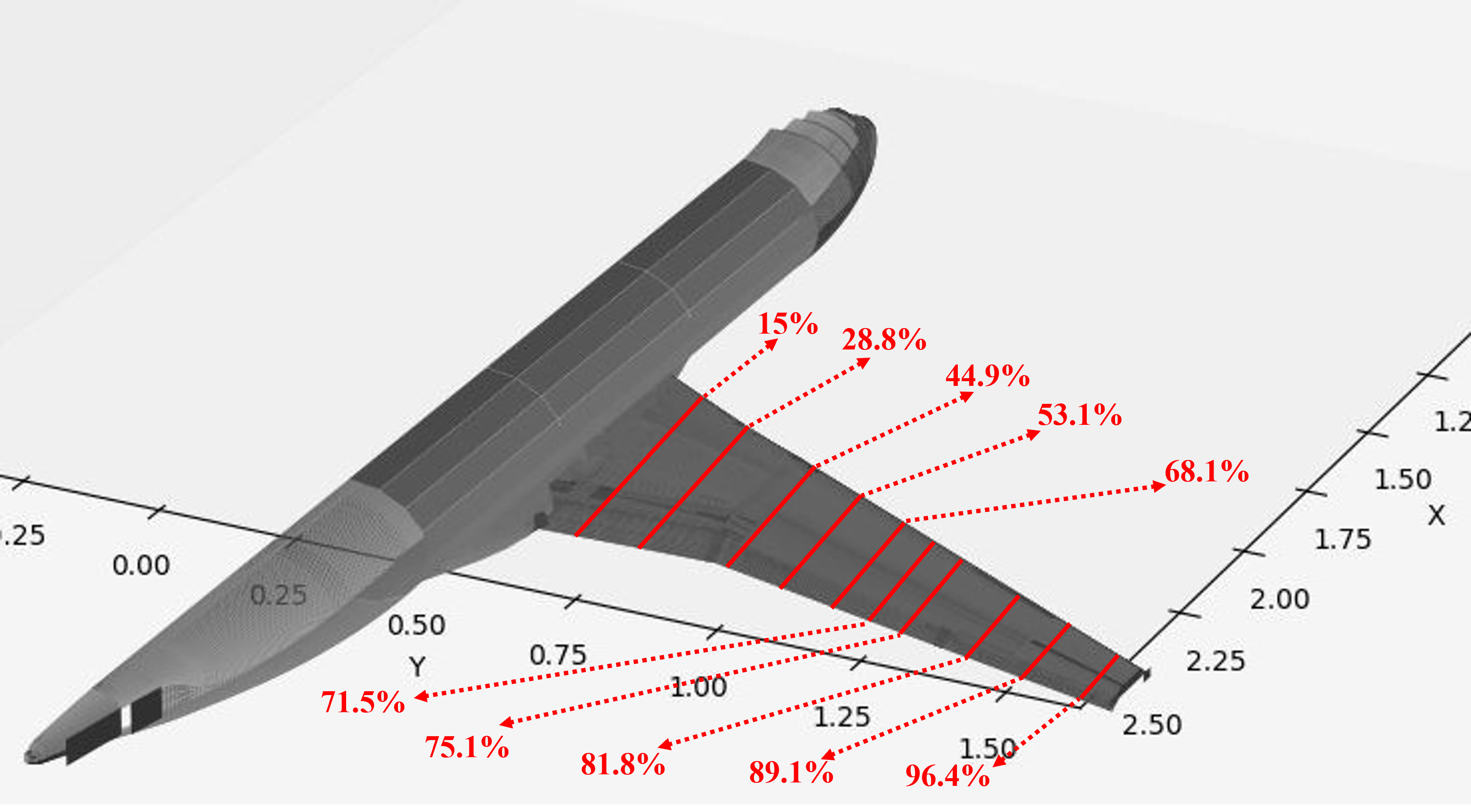
The geometry part provides the shape of a half fuselage with a wing in the form of polynomial surface control points in 3D space. By (1), a smooth manifold is constructed based on a part of DLR-F11 control points. Multiple smooth manifolds can be concatenated as a piecewise smooth manifold $\mathcal{M}$ to represent the entire geometry of DLR-f11 aircraft. The geometry part also provides coordinate points with 10 different span width configurations for $C_{P}$ measurement. The piecewise smooth manifold $\mathcal{M}$ and the span width configurations are shown in Fig. 3. For arbitrary point $P_{ab}\in\mathcal{M}$, geometric features ($g_{ij}$, $\mit\Gamma_{ij}^{k}$ and $S$) can be calculated by (4), (6) and (9), respectively. The dimensions of these geometric features are shown as in Table 1.

Table 1: Dimensions of geometric features.

parameter	Riemannian metric	connection	curvature
dimension	matrix($2\times 2$)	matrix($2\times 2\times 2$)	scalar(1)

The flight condition part describes different flight status of DLR-F11 aircraft, the parameters and their variations are shown as in Table 2. The aerodynamic coefficient is $C_{P}$.

Table 2: Flight conditions in DLR-F11 aircraft dataset.

parameters	$AoA$	$Ma$	$Re$
optional value	0°,7°,12°,16°,18°, 18.5°,19°,20°,21°	0.175	$1.35\times 10^{6}$

4.2 Model settings

In this section, we introduce the structure and the input data of MTL, MDF, our method, MLP and DAN.

Table 3: The optimal structure of comparative models. The symbol “k” denotes “kernel”, and “s” denotes “stride”.

model	input data	the optimal structure
MTL	$\vec{\mathbf{x}}_{1},\vec{\mathbf{x}}_{2}$	$f_{1}$:FC:$16\times 3$ $f_{2}$:FC:$16\times 3$ $c$:FC:$16\times 3$
MDF	$\vec{\mathbf{x}}_{1},\vec{\mathbf{x}}_{2},\vec{\mathbf{x}}_{3},$ $\vec{\mathbf{x}}_{4},\vec{\mathbf{x}}_{5}$	$f_{1}$:FC:$16\times 3$ $f_{2}$:FC:$16\times 3$ $f_{3}$: CV:k=$2\times 2\times 4$,s=$2\times 2$; CV:k=$2\times 2\times 8$,s=$2\times 2$; CV:k=$2\times 2\times 16$,s=$2\times 2$; $f_{4}$: CV:k=$2\times 2\times 4$,s=$2\times 2$; CV:k=$2\times 2\times 8$,s=$2\times 2$; CV:k=$2\times 2\times 16$,s=$2\times 2$; $f_{5}$:FC:$16\times 3$ $c$:FC:$32\times 3$
Our method	$9\times\{\vec{\mathbf{x}}_{1},\vec{\mathbf{x}}_{2},$ $\vec{\mathbf{x}}_{3},\vec{\mathbf{x}}_{4},\vec{\mathbf{x}}_{5}\}$	$f_{1}$:FC:$16\times 3$ $f_{2}$: CV:k=$2\times 2\times 4$,s=$2\times 2$; CV:k=$2\times 2\times 8$,s=$2\times 2$; CV:k=$2\times 2\times 16$,s=$2\times 2$; $f_{3}$: CV:k=$2\times 2\times 4$,s=$2\times 2$; CV:k=$2\times 2\times 8$,s=$2\times 2$; CV:k=$2\times 2\times 16$,s=$2\times 2$; $f_{4}$: CV:k=$2\times 2\times 4$,s=$2\times 2$; CV:k=$2\times 2\times 8$,s=$2\times 2$; CV:k=$2\times 2\times 16$,s=$2\times 2$; $f_{5}$:FC:$16\times 3$ $c$:FC:$16\times 3$
MLP	$9\times\{\vec{\mathbf{x}}_{1},\vec{\mathbf{x}}_{2},$ $\vec{\mathbf{x}}_{3},\vec{\mathbf{x}}_{4},\vec{\mathbf{x}}_{5}\}$	FC:$128\times 6$
DAN	wing section image, $\vec{\mathbf{x}}_{1}$	FC:$128\times 6$

Flight conditions, coordinates on the wing surface, and geometric features are different types of data, and their numerical value, distribution, and physical meaning are different. It has been demonstrated that using a context network to learn the weight vector to fuse $f_{z\alpha}(\vec{\mathbf{x}}_{z})$ outputs more accurate predicted coefficients than with directly concatenates $\vec{\mathbf{x}}_{1}\sim\vec{\mathbf{x}}_{5}$ as inputs [18, 19, 20]. In this paper, MTL, MDF and our method use a weight vector mechanism to predict $C_{P}$, MLP concatenates $\vec{\mathbf{x}}_{1}\sim\vec{\mathbf{x}}_{5}$ as inputs to predict $C_{P}$, and DAN concatenates features extracted from wing section images and flight conditions together as inputs to predict $C_{P}$.

Considering that the above models contain fully connected (FC) layers and convolutional (CV) layers, we design multiple structures for each model according to the number of FC layers, CV layers and hidden nodes. The optional numbers of CV and FC layers are 3 and 6, respectively. For FC layers, the optional numbers of hidden nodes are 16, 32, 64 and 128. For CV layers, the kernel size are $2\times 2$, the channel of each kernel is $2^{1+e}$, where $e$ denotes the sequence number of each CV layer ($e$ starts from 1). For MTL, MDF and our method, the number of hidden layers in each function network are the same (for example, if the function network_1 has 3 layers, the remaining function networks also have 3 hidden layers). Therefore, MTL, MDF and our method have 64 different structures, respectively. MLP and DAN have 8 different structures, respectively. Table 3 only introduce the structures with smallest test errors (the optimal structure).

MTL takes flight conditions $\vec{\mathbf{x}}_{1}$ and coordinates $\vec{\mathbf{x}}_{2}$ as inputs to predict $C_{P}$. The function network_1, taking $\vec{\mathbf{x}}_{1}$ as input, has 3 hidden layers, each of which has 16 nodes, i.e., the structure of function network_1 is set to “FC: $16\times 3$”. The function network_2 takes $\vec{\mathbf{x}}_{2}$ (with shape $batchsize\times 3$) as input, the structure of function network_2 is set to “FC: $16\times 3$”. In addition, the context network takes $[\vec{\mathbf{x}}_{1},\vec{\mathbf{x}}_{2}]$ as input, and the structure of the context network is set to “FC: $16\times 3$”.

MDF in [18] takes $\vec{\mathbf{x}}_{1}$, $\vec{\mathbf{x}}_{2}$ and $\vec{\mathbf{x}}_{3}$ as inputs to predict $C_{L}$ and $C_{D}$. In this experiment, MDF takes $\vec{\mathbf{x}}_{1}$, $\vec{\mathbf{x}}_{2}$ and geometric features ($\vec{\mathbf{x}}_{3}$, $\vec{\mathbf{x}}_{4}$, and $\vec{\mathbf{x}}_{5}$) as inputs to predict $C_{P}$. The function network_1 takes $\vec{\mathbf{x}}_{1}$ as input, and the function network_2 takes $\vec{\mathbf{x}}_{2}$ as input. The structures of function network_1 and function network_2 in MDF are identical to those of function network_1 and function network_2 in MTL. The function network_3 that takes $\vec{\mathbf{x}}_{3}$ (with shape $batchsize\times 1\times 2\times 2$) as input is designed as a 2D CNN. The function network_3 consists of three convolutional layers, each of which have a convolution kernel with shape $2\times 2\times 4$, $2\times 2\times 8$ and $2\times 2\times 16$, respectively. The function network_4 takes $\vec{\mathbf{x}}_{4}$ (with shape $batchsize\times 2\times 2\times 2$) as input. The structure of function network_4 is the same with the structure of function network_3. The stride of all kernels is $2\times 2$. Because $\vec{\mathbf{x}}_{5}$ is a vector with shape $batchsize\times 1$, the structure of the function network_5 is set to “FC: $16\times 3$”. In addition, the structure of the context network is set to “FC: $32\times 3$”.

Figure 4: Vertical and horizontal Euclidean distance among neighbors.

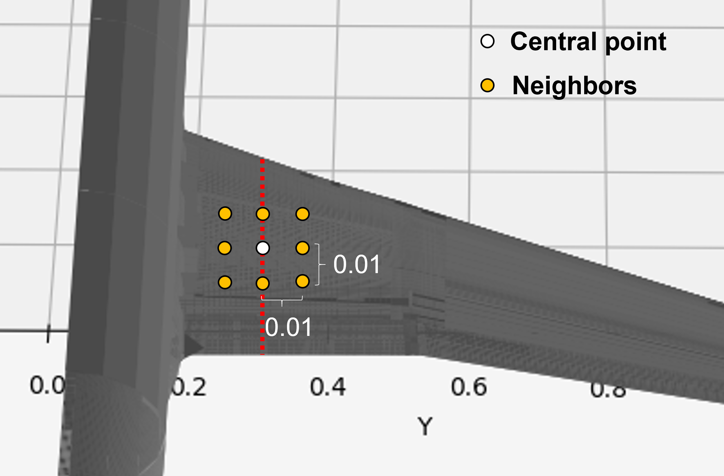
Our method additionally considers geometric features from 8 neighbors around point $P_{ab}$. Fig. 4 describes how to select the 8 neighbors on the DLR-F11 wing. Among the 9 points, the distance $d=0.01$. The input of function network_2 is a matrix (with shape $batchsize\times 1\times 9\times 3$) that contains 9 different $\vec{\mathbf{x}}_{2}$, therefore the function network_2 is a 2D CNN, which consists of three convolutional layers, each of which have a convolution kernel with shape $2\times 2\times 4$, $2\times 2\times 8$ and $2\times 2\times 16$, respectively. Similarly, the inputs of the function network_3 (with shape $batchsize\times 1\times 18\times 2$), function network_4 (with shape $batchsize\times 2\times 18\times 2$) and function network_5 (with shape $batchsize\times 9$) are also matrices contain 9 different $\vec{\mathbf{x}}_{3}$, $\vec{\mathbf{x}}_{4}$ and $\vec{\mathbf{x}}_{5}$, respectively. The structures of function network_1, function network_5 and context network are all set to “FC: $16\times 3$”.

The input data of MLP is exactly the same with our method. The MLP is a multi-layer perceptron with 3 layers and each layer has 128 nodes. The aim of comparing MLP with MTL, MDF and our method is to further verify the effectiveness of the weight vector mechanism. Because the source code of MLP is not published by [49], we implemented MLP for this experiment.

DAN takes wing section images with different span width and $\vec{\mathbf{x}}_{1}$ as input to predict $C_{P}$. DAN consists of two parts, a pre-trained Transformer encoder and a MLP. The pre-trained transformer encoder is used to extract latent features (with shape $batchsize\times 1000$) from airfoil images. The input of the MLP in DAN is the concatenation of extracted features and $\vec{\mathbf{x}}_{1}$. The optimal MLP in DAN has 6 layers and each of which has 128 nodes .

Table 4: Parameters of all models in this paper.

parameter	value
optimization algorithm	Adam(Beta1=0.9 and Beta2=0.999)[50]
data normalization	max-min normalization
activation function	ReLU [51]
batch size	470
learning rate	0.001
epochs	2000
validation	7-fold cross validation

Table 5: Average MSEs of MTL, MDF, our method, MLP and DAN. The average MSE reduction is calculated as the average value for each MSE reduction with different $AoA$.

$AoA$	MTL [48]	MDF [18]	Our method	MLP [49]	DAN [25]	MSE reduction (our mehod V.S. DAN)
7°	$1.49$	$1.53$	$\mathbf{1.46}$	$1.53$	$1.52$	3.95%
12°	$\mathbf{1.19}$	$1.21$	$1.23$	$1.21$	$1.21$	-1.65%
16°	$8.26\times 10^{-1}$	$6.66\times 10^{-1}$	$6.54\times 10^{-1}$	$\mathbf{5.93\times 10^{-1}}$	$6.50\times 10^{-1}$	-0.62%
18°	$3.31\times 10^{-1}$	$2.92\times 10^{-1}$	$\mathbf{2.03\times 10^{-1}}$	$2.22\times 10^{-1}$	$2.29\times 10^{-1}$	11.35%
18.5°	$2.22\times 10^{-1}$	$1.82\times 10^{-1}$	$1.50\times 10^{-1}$	$\mathbf{1.36\times 10^{-1}}$	$1.56\times 10^{-1}$	3.85%
19°	$1.71\times 10^{-1}$	$2.08\times 10^{-1}$	$\mathbf{7.72\times 10^{-2}}$	$1.99\times 10^{-1}$	$7.98\times 10^{-2}$	3.26%
20°	$1.70\times 10^{-1}$	$6.94\times 10^{-2}$	$\mathbf{1.41\times 10^{-2}}$	$1.82\times 10^{-2}$	$2.30\times 10^{-2}$	38.70%
average	$6.29\times 10^{-1}$	$5.94\times 10^{-1}$	$\mathbf{5.41\times 10^{-1}}$	$5.58\times 10^{-1}$	$5.53\times 10^{-1}$	8.41%

The parameters of all models compared in this paper are shown in Table 4. The MSE are chosen as an assessment indicator for the predicted $C_{P}$:

$$MSE=\frac{1}{M}\sum_{\beta=1}^{M}\left(C_{P_{te}}^{\beta}-\hat{C}_{P}^{\beta}\right)^{2}$$

where $C_{P_{te}}^{\beta}$ denotes the true $C_{P}$ value of the $\beta$th sample in the test set, and $\hat{C}_{P}^{\beta}$ denotes the predicted value of the $\beta$th sample in the test set.

Figure 5: Training and validation loss corves for MTL, MDF, our method, MLP and DAN with $AoA=20$°.

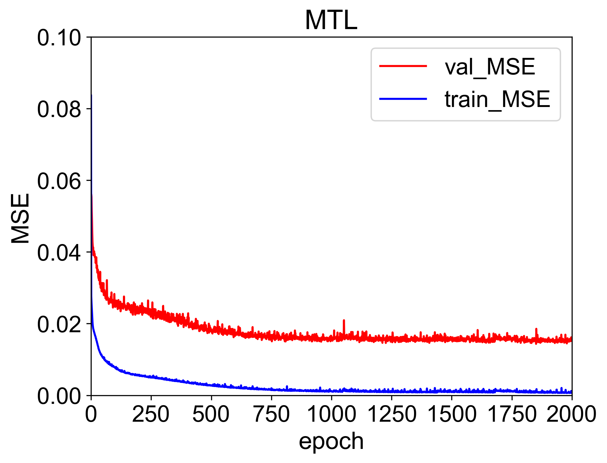
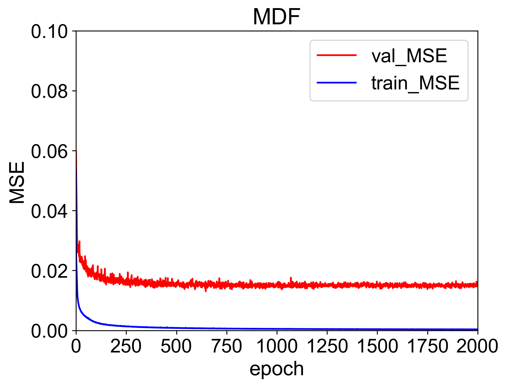
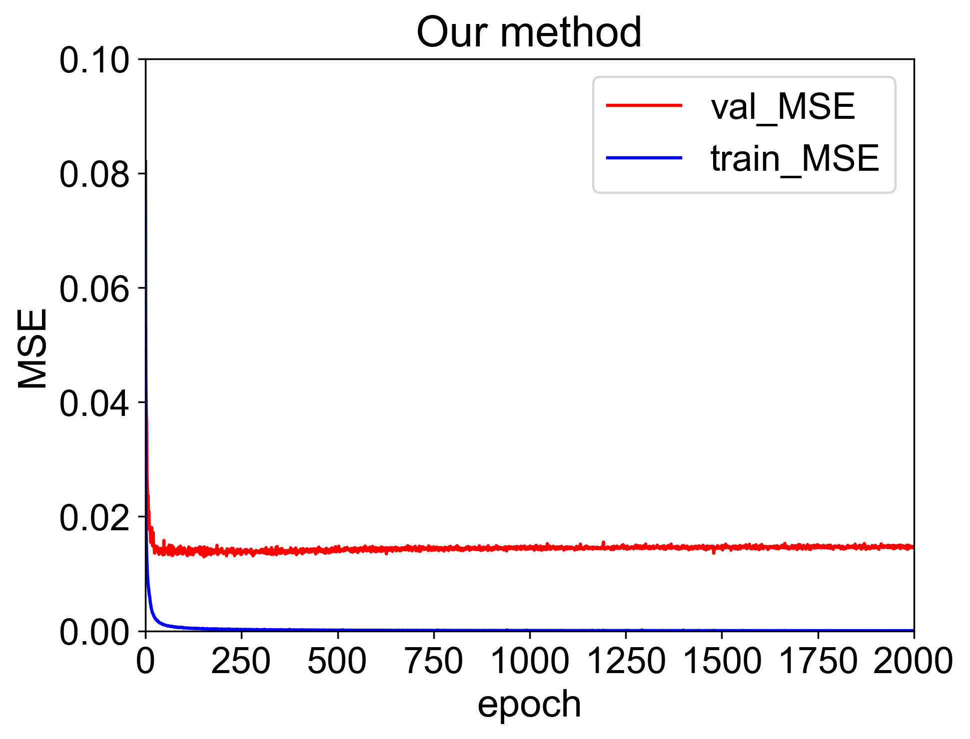
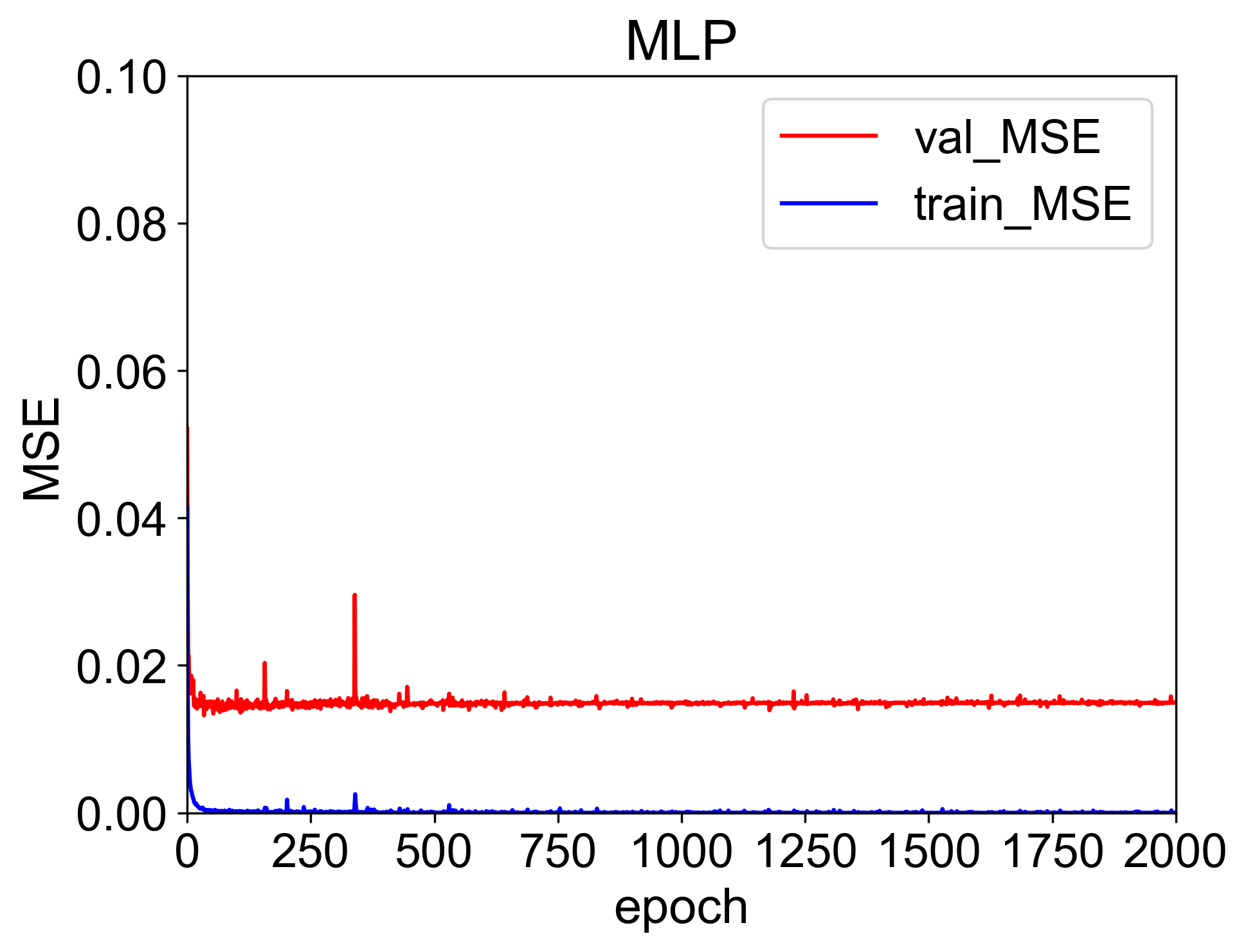
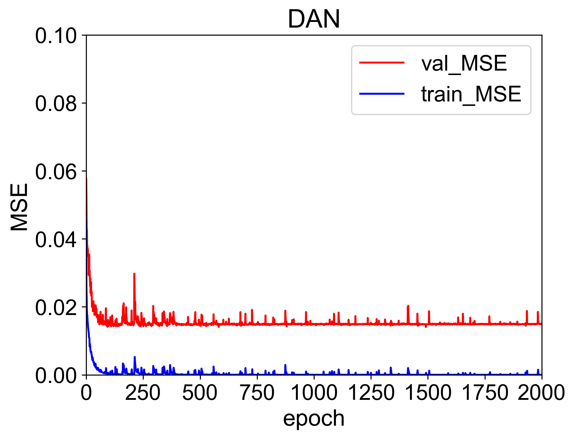
All models in this paper are verified by a 7-fold cross-validation. The test set of each fold experiment in the 7-fold cross-validation contains all the samples with a specific $AoA$, and the samples related to this $AoA$ do not appear in the training set. For example, in the first-fold of the 7-fold cross-validation, all the data samples with $AoA=7$° are selected as the first test set, the remaining sample are selected as the first training set. In the second-fold of the 7-fold cross-validation, all the samples with $AoA=12$° are selected as the second test set, the remaining sample are selected as the second training set. The remaining folds of the 7-fold cross-validation are similar.

4.3 Results and analysis

Figure 6: The predicted $C_{P}$ (a) and predicted errors (b) with $AoA=20$° and span width equals 15%. The horizontal axis denotes the x axis along the fuselage direction, and the vertical axis denotes the z axis along the fuselage normal direction.

Figure 7: The predicted $C_{P}$ (a) and predicted errors (b) with $AoA=20$° and span width equals 68.1%. The horizontal and vertical axes have the same meanings as depicted in Fig. 6.

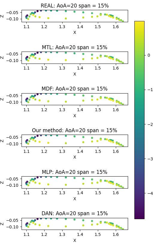
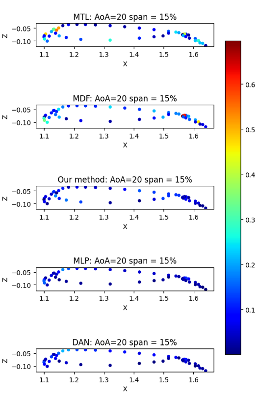
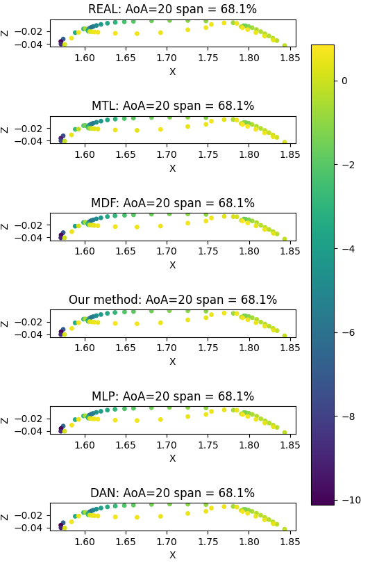
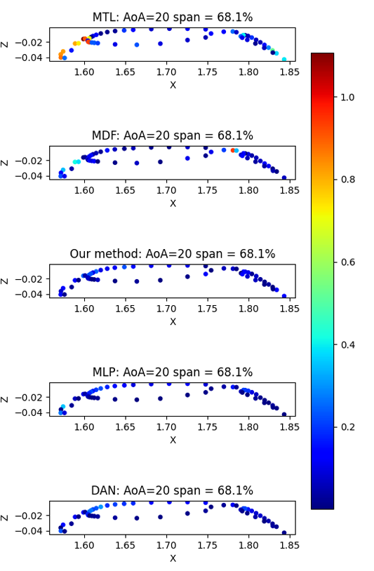
Table 5 displays the average test MSEs for MTL, MDF, our method, MLP and DAN. In every row, figures in bold represent the minimum test MSEs (all the test MSEs are not normalized). Generally, the test MSEs of $C_{P}$ predicted by all models decrease as the $AoA$ increases. This phenomenon occurs because the data samples in the large $AoA$ region are densely populated, whereas the data samples in the small $AoA$ region are relatively sparse. Comparing our method with DAN under the condition of $12$°$\leq AoA\leq 16$°, DAN exhibits smaller prediction MSEs than our method. However, for $AoA\geq 18$°, the prediction MSEs of DAN are bigger than those of our method. Similarly, when comparing our method with MLP, MLP shows smaller prediction MSEs at $AoA=16$° and $AoA=18.5$°, while our method exhibits smaller prediction MSEs for $AoA\geq 19$°. The above observations indicate that our method is more accurate in predicting $C_{P}$ than other models for large $AoA$. Conversely, MLP and DAN have advantages in the case of relatively small $AoA$.

Fig. 5 depicts the average training and validation corves for all the above models in the 7-fold experiments. The fluctuations in loss variations observed in subgraphs (a), (d) and (e) are larger than those in other subgraphs. This indicates a difference in the stability of the training processes. The models corresponding to subgraphs (b) and (c) (MDF and our method) are more stable. Furthermore, compared with subgraph (a), the models represented in subgraphs (b), (c), and (d) (MDF, our method, and MLP) converge faster than MTL. These three models all incorporate geometric features as part of their inputs, which suggests that the incorporation of geometric features accelerates the convergence of their training processes. It’s worth highlighting that the models corresponding to subgraphs (c) and (d) (our method and MLP) incorporate the geometric features from additional 8 neighbors as part of their inputs, which further accelerates the convergence of these two models.

Figure 8: The predicted errors with $AoA=18$° (a) and $AoA=7$° (b), and span width equals 68.1%. The horizontal and vertical axes have the same meanings as depicted in Fig. 6.

Figure 9: The $C_{P}$ variations of test set, our method, MLP and DAN with $AoA=20$°. The horizontal axis denotes the x axis along the fuselage direction, and the vertical axis denotes $C_{P}$ value.

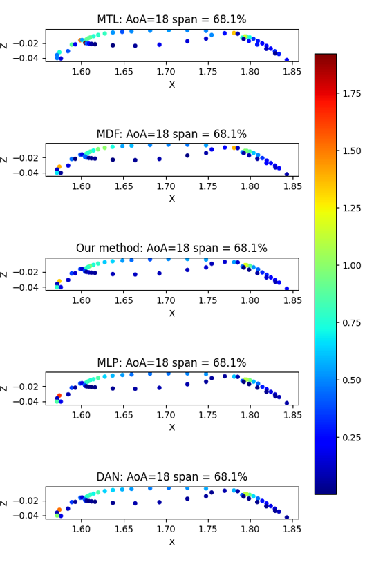
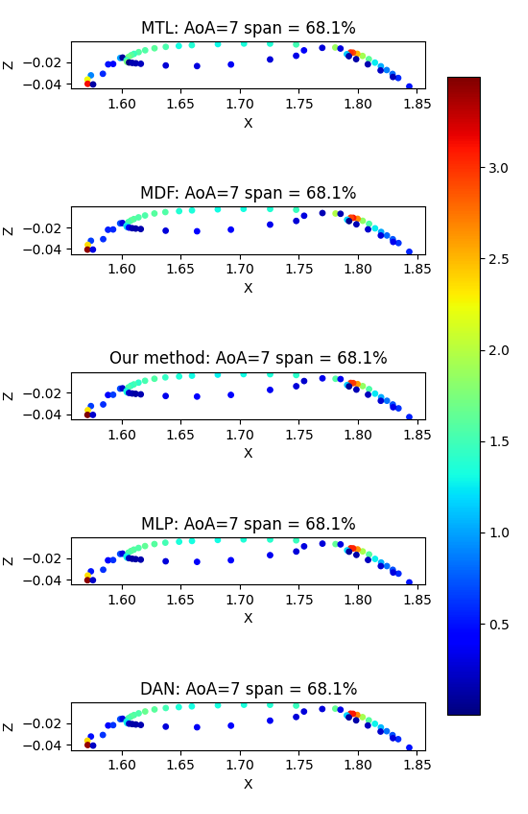
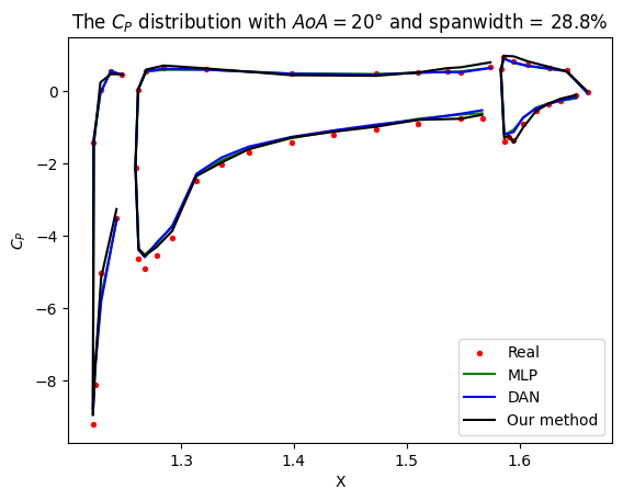
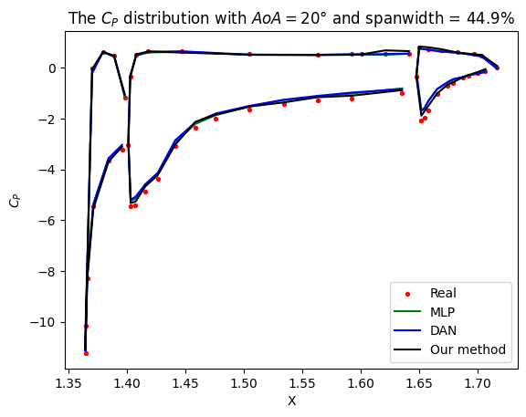
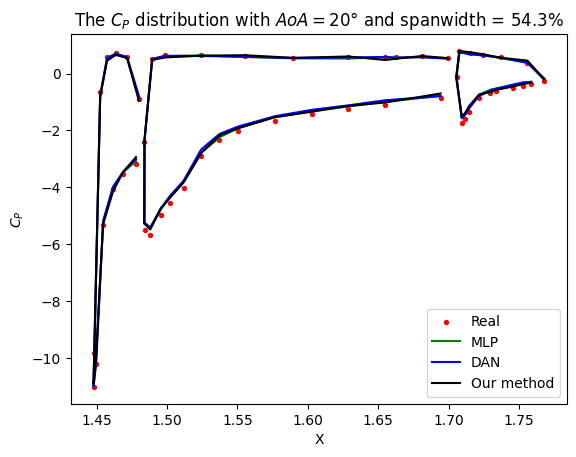
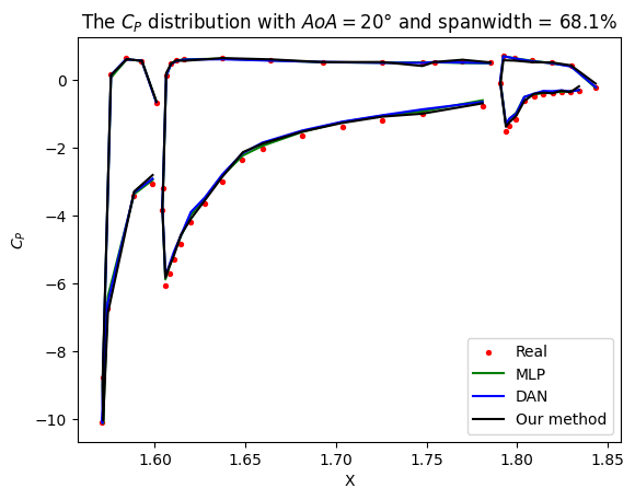
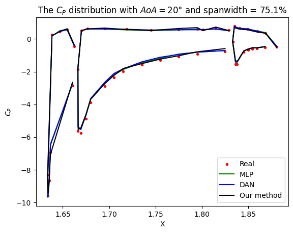
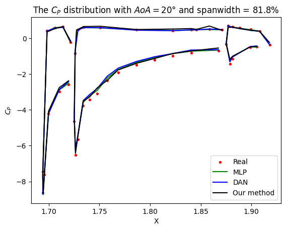
Fig. 6 illustrates the predicted $C_{P}$ distributions and the corresponding prediction errors on the surface of DLR-F11 wing with $AoA=20$° and span width equals 15%. The DLR-F11 aircraft contains a three-stage wing, it is evident that the wing sections depicted in the graph are composed of three parts. In each row of every subgraph, the left part represents the first wing stage, the middle part represents the second wing stage, and the right part denotes the third wing stage. In subgraph (a), the $C_{P}$ distributions predicted by all models are similar, suggesting that each model is capable of learning the variations in $C_{P}$ distribution on the DLR-F11 wing surface. To clearly compare the details of the predicted $C_{P}$ values in subgraph (a), we calculate

$$err^{\beta}=|C_{P_{te}}^{\beta}-\hat{C}_{P}^{\beta}|$$ (15)

where $err^{\beta}$ denotes the prediction error of the $\beta$th sample, $C_{P_{te}}^{\beta}$ denotes the real $C_{P}$ value of the $\beta$th sample in the test set, and $\hat{C}_{P}^{\beta}$ denotes the predicted value of the $\beta$th sample in the test set. The $err^{\beta}$ of each model is plotted in subgraph (b). On the first wing stage, all the points generated by MTL and MDF show larger errors compared to the points generated by our method. At the leading edge on the first wing stage, the points generated by MTL, MDF, MLP and DNA also show larger errors than the points generated by our method. At the leading edge on the upper surface of the second wing stage, the points generated by MTL, MDF, MLP and DAN exhibit larger errors than the points generated by our method. The leading edge of a wing is the area where its $C_{P}$ changes dramatically, and our method is more accurate at the leading edge of both the first and second stages than other models. At the trailing edge on the upper surface of the second wing stage, the points generated by MTL, MDF, our method and DAN have larger errors than the points generated by MLP. On the lower surface of the second wing stage, the points generated by MTL, MDF, our method are not as accurate as the points generated by MLP and DAN. At the leading edge on the third wing stage, the points generated by MTL, MDF, MLP and DAN have larger errors than the points generated by our method. These observations demonstrate that our method is more accurate at the leading edge of wing sections than other methods.

Fig. 7 illustrates the predicted $C_{P}$ distributions and the corresponding prediction errors on the surface of DLR-F11 wing with $AoA=20$° and span width equals 68.1%. Similar to Fig. 6, subgraph (a) demonstrates that all models can learn the variations of $C_{P}$ distributions. In subgraph (b), on the first wing stage, the points generated by MTL, MDF and MLP have larger errors than the points generated by our method and DAN. At the leading edge on the second wing stage, the points generated by MLP, DAN have larger errors than the points generated by MTL, MDF and our method. At the trailing edge of the second wing stage, one point generated by MDF is red. However, among all corresponding points generated by these comparative models, the points generated by our method have the darkest color, indicating that the $C_{P}$ error of this point predicted by our method is the smallest among the comparative models in this paper. On the third wing stage, the points generated by MTL show larger errors than the points generated by other methods. These observations demonstrate that our method is more accurate at the leading edge on the first wing stage than other methods.

Figure 10: The $C_{P}$ variations of test set, our method, MLP and DAN with $AoA=18.5$°. The horizontal and vertical axes have the same meanings as depicted in Fig. 9.

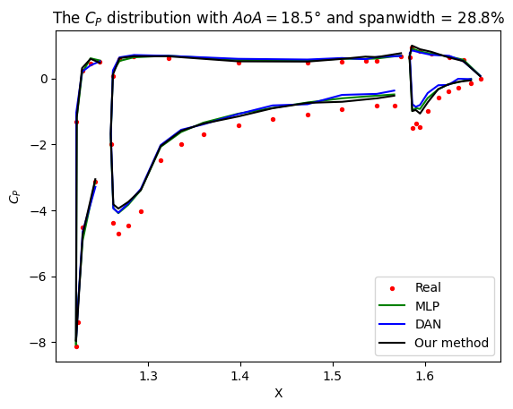
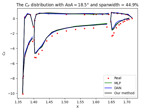
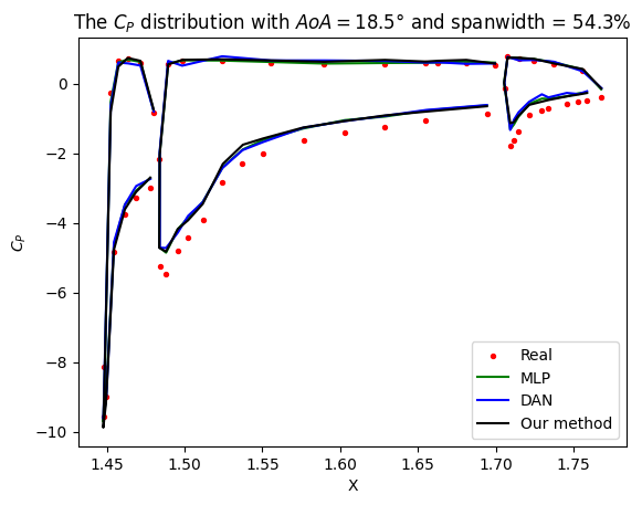
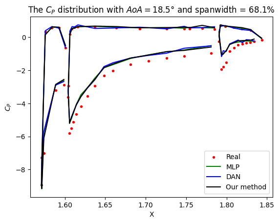
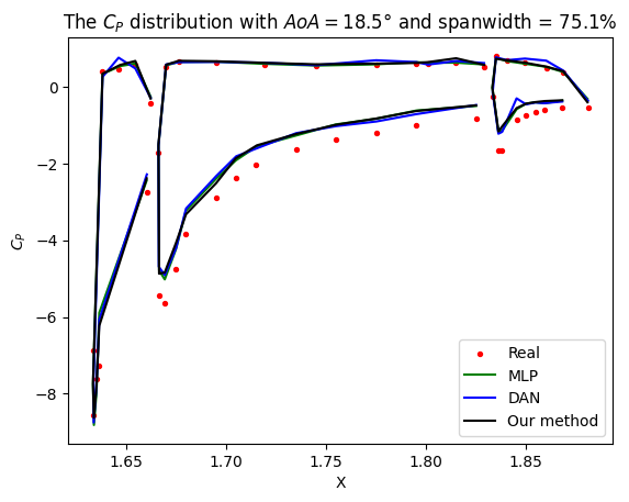
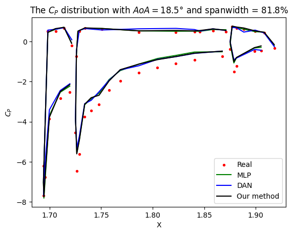
Fig. 8 displays the prediction errors of the DLR-F11 wing section with a span width of 68.1% at $AoA$ of 18° and 7°, respectively. In subgraph (a), at the leading edge on the first wing stage, the points generated by MDF, MLP and DAN show larger errors than the points generated by MTL and our method. The remaining stages are similar. In subgraph (b), it is difficult to see the differences among the models in detail. In addition, points on the upper surface of the second wing stage generated by all methods have large errors, because the DLR-F11 data samples in small $AoA$ region are sparser than those in large $AoA$. The observations in Fig. 6, Fig. 7 and Fig. 8 demonstrate that our method exhibits distinct advantages at the leading edge of wing sections in case with large $AoA$, while in cases with small $AoA$, our method closely aligns with existing methods, which is consistent with table 5.

To better illustrate $C_{P}$ variations of different models, the $C_{P}$ variations of different wing sections at different $AoA$ are plotted in Fig. 9 and Fig. 10. It is worth noting that only three models (our method, MLP and DAN) are included to maintain clarity in graphs, as they exhibit relatively small prediction errors. In each subgraph, three set of curves are plotted to depict the $C_{P}$ variations on three stages of the DLR-F11 wing. The left curve represents the $C_{P}$ variation on the first wing stage, the middle curve represents the $C_{P}$ variation on the second wing stage, and the right curve represents the $C_{P}$ variation on the third wing stage. In each curve, the upper curve represents the $C_{P}$ variations on the lower surface of the DLR-F11 wing, and the lower curve represents the $C_{P}$ variations on the upper surface of the DLR-F11 wing.

Fig. 9 displays the $C_{P}$ variations of multiple wing sections with span width of 28.8%, 44.9%, 54.3%, 68.1%, 75.1%, and 81.8% at $AoA$ of 20°. In subgraphs (a) and (b), the black curves closely align with the red points in the lower part of each curve, indicating that our method effectively captures the $C_{P}$ variations on the upper surface of the DLR-F11 wing. In subgraphs (c) and (d), all curves exhibit similar variations. In subgraphs (e) and (f), the black curves at the first and third wing stage closely match the red points. The black lower curve of the second wing stage are closer to red points than other curves. In addition, only one or two points in the black upper curve are inaccurate, and the remaining points are accurate. In general, our method accurately predicts $C_{P}$ variations on the first and third wing stage, as well as on the upper surface of the second wing stage. However, our method are inaccurate in predicting $C_{P}$ value of few points on the lower surface of the second wing stage (Notice: the upper curve in Fig. 9 denotes the $C_{P}$ variations on the lower surface of the DLR-F11 wing, and the lower curve denotes the $C_{P}$ variations on the upper surface of the DLR-F11 wing).

Fig. 10 illustrates $C_{P}$ variations of the same wing sections with the same span widths at $AoA=18.5$°. In subgraphs (a) and (b), the lower part of the blue curves of the third wing stage exhibits a zigzag pattern. In contrast, the black curves in the corresponding region are relatively smooth. This observation indicates that DAN is difficult to accurately predict the $C_{P}$ variation on the upper surface of the third wing stage, while our method can predict more accurate $C_{P}$ variations than DAN in this region. The green curves almost coincide with the black curves. However, comparing the lower parts of the second and third wing stage, it is evident that MLP is not as accurate as our method. In subgraphs (c) to (f), the zigzag pattern of the blue curves are more obvious, especially within the curves corresponding to the third wing stage. These observations suggest that the geometric features proposed in this paper offer a more accurate representation of 3D wings than images (DAN use images of wing sections to predict the $C_{P}$ distributions of the DLR-F11 wing).

5 CONCLUSION

In this paper, we propose a learning method that incorporating Riemannian geometric features for predicting the $C_{P}$ distributions on wing surfaces in 3D space. We demonstrate that the geometry of a wing in 3D space can be described by a set of self-intersection-free Bézier surfaces, and further demonstrate that three geometric features (Riemannian metric, connection and curvature) can be used to represent the geometric structure of a wing in 3D space. The experimental results show that our method which incorporating the geometric features from 9 points (including the additional 8 neighbors) into the multi-feature learning module reduces the average prediction MSE of $C_{P}$ by 8.41% for the DLR-F11 aircraft test set.

[]Liwei Hu received a B.S. degree in software engineering from the School of Software, Hebei Normal University, Shijiazhuang, Hebei, China, in 2014, as well as an M.S. degree in computer technology from the University of Electronic Science and Technology of China (UESTC), Chengdu, Sichuan, China, in 2018. He is currently pursuing a Ph.D. degree in computer science and technology from the School of Computer Science and Engineering, UESTC. His research fields include aerodynamic data modeling, deep learning and pattern recognition.

[]Wenyong Wang received a B.S. degree in computer science from BeiHang University, Beijing, China, in 1988 and M.S. and Ph.D. degrees from the University of Electronic Science and Technology (UESTC), Chengdu, China, in 1991 and 2011, respectively. He has been a professor in computer science and engineering at UESTC since 2006. He is also a special-term professor at Macau University of Science and Technology, a senior member of the Chinese Computer Federation, a member of the expert board of the China Education and Research Network (CERNET) and China next generation internet. His main research interests include next generation Internet, software-defined networks, and software engineering.

[]Yu Xiang received B.S, M.S. and Ph.D. degrees from the University of Electronic Science and Technology of China (UESTC), Chengdu, Sichuan, China, in 1995, 1998 and 2003, respectively. He joined the UESTC in 2003 and became an associate professor in 2006. From 2014-2015, he was a visiting scholar at the University of Melbourne, Australia. His current research interests include computer networks, intelligent transportation systems and deep learning.

[]Stefan Sommer received his M.S. in mathematics in 2008, and his Ph.D. in computer science in 2012 from the University of Copenhagen. He is currently Professor at the Department of Computer Science, University of Copenhagen. His research interests include shape analysis theory and applications in science and engineering, and statistics and machine learning on data with complex, geometric structure (geometric statistics).

References

- [1] R. Mukesh, K. Lingadurai, and U. Selvakumar, “Airfoil shape optimization using non-traditional optimization technique and its validation,” Journal of King Saud University-Engineering Sciences, vol. 26, no. 2, pp. 191–197, 2014.
- [2] N. Vu and J. Lee, “Aerodynamic design optimization of helicopter rotor blades including airfoil shape for forward flight,” Aerospace Science and Technology, vol. 42, pp. 106–117, 2015.
- [3] G. Liu, F. Gao, and W.-H. Liao, “Design and optimization of a magnetorheological damper based on b-spline curves,” Mechanical Systems and Signal Processing, vol. 178, p. 109279, 2022.
- [4] B. Song, Z. Wang, and L. Zou, “An improved pso algorithm for smooth path planning of mobile robots using continuous high-degree bezier curve,” Applied Soft Computing, vol. 100, p. 106960, 2021.
- [5] M. Saporito, A. Da Ronch, N. Bartoli, and S. Defoort, “Robust multidisciplinary analysis and optimization for conceptual design of flexible aircraft under dynamic aeroelastic constraints,” Aerospace Science and Technology, vol. 138, p. 108349, 2023.
- [6] Q. Zhao, “Airfoil inverse design based on particle swarm optimization algorithm,” in Fifth International Conference on Computer Information Science and Artificial Intelligence (CISAI 2022), vol. 12566. SPIE, 2023, pp. 1080–1085.
- [7] E. Abele and M. Fujara, “Simulation-based twist drill design and geometry optimization,” CIRP annals, vol. 59, no. 1, pp. 145–150, 2010.
- [8] G. Papacharalampous, H. Tyralis, S. M. Papalexiou, A. Langousis, S. Khatami, E. Volpi, and S. Grimaldi, “Global-scale massive feature extraction from monthly hydroclimatic time series: Statistical characterizations, spatial patterns and hydrological similarity,” Science of the Total Environment, vol. 767, p. 144612, 2021.
- [9] N. Decat, J. Walter, Z. H. Koh, P. Sribanditmongkol, B. D. Fulcher, J. M. Windt, T. Andrillon, and N. Tsuchiya, “Beyond traditional sleep scoring: Massive feature extraction and data-driven clustering of sleep time series,” Sleep Medicine, vol. 98, pp. 39–52, 2022.
- [10] H. Zhang, M. Hao, H. Wu, H.-F. Ting, Y. Tang, W. Xi, and Y. Wei, “Protein residue contact prediction based on deep learning and massive statistical features from multi-sequence alignment,” Tsinghua Science and Technology, vol. 27, no. 5, pp. 843–854, 2022.
- [11] D. Hegde, J. M. J. Valanarasu, and V. M. Patel, “Clip goes 3d: Leveraging prompt tuning for language grounded 3d recognition,” arXiv preprint arXiv:2303.11313, 2023.
- [12] S. Qi, X. Ning, G. Yang, L. Zhang, P. Long, W. Cai, and W. Li, “Review of multi-view 3d object recognition methods based on deep learning,” Displays, vol. 69, p. 102053, 2021.
- [13] S. Y. Alaba and J. E. Ball, “Deep learning-based image 3-d object detection for autonomous driving,” IEEE Sensors Journal, vol. 23, no. 4, pp. 3378–3394, 2023.
- [14] S. Yang, S. Lee, and K. Yee, “Inverse design optimization framework via a two-step deep learning approach: application to a wind turbine airfoil,” Engineering with Computers, vol. 39, no. 3, pp. 2239–2255, 2023.
- [15] X. Du, P. He, and J. R. Martins, “A b-spline-based generative adversarial network model for fast interactive airfoil aerodynamic optimization,” in AIAA Scitech 2020 Forum, 2020, p. 2128.
- [16] R. Zahn, A. Weiner, and C. Breitsamter, “Prediction of wing buffet pressure loads using a convolutional and recurrent neural network framework,” CEAS Aeronautical Journal, pp. 1–17, 2023.
- [17] D. Hines and P. Bekemeyer, “Graph neural networks for the prediction of aircraft surface pressure distributions,” Aerospace Science and Technology, vol. 137, p. 108268, 2023.
- [18] Y. Xiang, L. Hu, G. Zhang, J. Zhang, and W. Wang, “A manifold-based airfoil geometric-feature extraction and discrepant data fusion learning method,” IEEE Transactions on Aerospace and Electronic Systems, 2023.
- [19] Z. Deng, J. Wang, H. Liu, H. Xie, B. Li, M. Zhang, T. Jia, Y. Zhang, Z. Wang, and B. Dong, “Prediction of transonic flow over supercritical airfoils using geometric-encoding and deep-learning strategies,” arXiv preprint arXiv:2303.03695, 2023.
- [20] Y. Wang, K. Shimada, and A. Barati Farimani, “Airfoil gan: encoding and synthesizing airfoils for aerodynamic shape optimization,” Journal of Computational Design and Engineering, vol. 10, no. 4, pp. 1350–1362, 2023.
- [21] J. G. Coder, “Overflow analysis of the dlr-f11 high-lift configuration including transition modeling,” Journal of Aircraft, vol. 52, no. 4, pp. 1082–1097, 2015.
- [22] G. Catalani, D. Costero, M. Bauerheim, L. Zampieri, V. Chapin, N. Gourdain, and P. Baqué, “A comparative study of learning techniques for the compressible aerodynamics over a transonic rae2822 airfoil,” Computers & Fluids, vol. 251, p. 105759, 2023.
- [23] S. J. Jacob, M. Mrosek, C. Othmer, and H. Köstler, “Deep learning for real-time aerodynamic evaluations of arbitrary vehicle shapes,” arXiv preprint arXiv:2108.05798, 2021.
- [24] J. Li and M. Zhang, “On deep-learning-based geometric filtering in aerodynamic shape optimization,” Aerospace Science and Technology, vol. 112, p. 106603, 2021.
- [25] K. Zuo, Z. Ye, W. Zhang, X. Yuan, and L. Zhu, “Fast aerodynamics prediction of laminar airfoils based on deep attention network,” Physics of Fluids, vol. 35, no. 3, 2023.
- [26] M. Selig, “Uiuc airfoil data site, department of aerospace engineering,” Urbana, Illinois: University of Illinois,(Jan 2007) www. ae. uiuc. edu/m-selig/ads. html. RL Fearn,“Airfoil Aerodynamics Using Panel Methods,” The Mathematica Journal, pp. 10–4, 2011.
- [27] K. Han, Y. Wang, H. Chen, X. Chen, J. Guo, Z. Liu, Y. Tang, A. Xiao, C. Xu, Y. Xu et al., “A survey on vision transformer,” IEEE transactions on pattern analysis and machine intelligence, vol. 45, no. 1, pp. 87–110, 2022.
- [28] X. Qu, Z. Liu, B. Yu, W. An, X. Liu, and H. Lyu, “Predicting pressure coefficients of wing surface based on the transfer of spatial dependency,” AIP Advances, vol. 12, no. 5, 2022.
- [29] R. Lei, J. Bai, H. Wang, B. Zhou, and M. Zhang, “Deep learning based multistage method for inverse design of supercritical airfoil,” Aerospace Science and Technology, vol. 119, p. 107101, 2021.
- [30] F. Xiong, L. Zhang, H. Xiao, and R. Chengkun, “A point cloud deep neural network metamodel method for aerodynamic prediction,” Chinese Journal of Aeronautics, vol. 36, no. 4, pp. 92–103, 2023.
- [31] B. Zhang, “Airfoil-based convolutional autoencoder and long short-term memory neural network for predicting coherent structures evolution around an airfoil,” Computers & Fluids, vol. 258, p. 105883, 2023.
- [32] Q. Chen, P. Pope, and M. Fuge, “Learning airfoil manifolds with optimal transport,” in AIAA SCITECH 2022 Forum, 2022, p. 2352.
- [33] A. Van Slooten and M. Fuge, “Effect of optimal geometries and performance parameters on airfoil latent space dimension,” in International Design Engineering Technical Conferences and Computers and Information in Engineering Conference, vol. 86229. American Society of Mechanical Engineers, 2022, p. V03AT03A005.
- [34] Y. Wang, K. Shimada, and A. B. Farimani, “Airfoil gan: Encoding and synthesizing airfoils foraerodynamic-aware shape optimization,” arXiv preprint arXiv:2101.04757, 2021.
- [35] L. Hu, Y. Xiang, J. Zhang, Z. Shi, and W. Wang, “Aerodynamic data predictions based on multi-task learning,” Applied Soft Computing, vol. 116, p. 108369, 2022.
- [36] J. Zhang, G. Zhang, Y. Cheng, L. Hu, Y. Xiang, and W. Wang, “A multi-task learning method for large discrepant aerodynamic data,” Acta Aerodynamica Sinica, vol. 40, pp. 64–72, 2022.
- [37] Z. Tang, “Metric,” in Fundamentals of Riemannian geometry in Chinese, 1st ed., C. Yue, Ed. Beijing: Beijing Normal University Publishing House, 2011, pp. 29–33.
- [38] J. M. Lee and J. M. Lee, Smooth manifolds. Springer, 2012.
- [39] w. Chen, “Riemannian metric,” in Introduction to Riemann geometry in Chinese, 1st ed., j. Zhang, Ed. Beijing: Beijing Normal University Publishing House, 2004, pp. 83–90.
- [40] X. Pennec, S. Sommer, and T. Fletcher, Riemannian geometric statistics in medical image analysis. Academic Press, 2019.
- [41] S. Sommer and A. Bronstein, “Horizontal flows and manifold stochastics in geometric deep learning,” IEEE transactions on pattern analysis and machine intelligence, vol. 44, no. 2, pp. 811–822, 2020.
- [42] A. T. Norkvist, “Projective real calculi and levi-civita connections,” arXiv preprint arXiv:2309.05191, 2023.
- [43] G. G. van der Vleuten, F. Toschi, W. H. Schilders, and A. Corbetta, “Stochastic fluctuations of diluted pedestrian dynamics along curved paths,” arXiv preprint arXiv:2306.12090, 2023.
- [44] V. Khatsymovsky, “On the discrete christoffel symbols,” International Journal of Modern Physics A, vol. 34, no. 30, p. 1950186, 2019.
- [45] S. Ivanov and N. Stanchev, “The riemannian bianchi identities of metric connections with skew torsion and generalized ricci solitons,” arXiv preprint arXiv:2307.03986, 2023.
- [46] H. Frost, C. R. Mafra, and L. Mason, “A lie bracket for the momentum kernel,” Communications in Mathematical Physics, vol. 402, no. 2, pp. 1307–1343, 2023.
- [47] O. Munteanu and J. Wang, “Comparison theorems for 3d manifolds with scalar curvature bound,” International Mathematics Research Notices, vol. 2023, no. 3, pp. 2215–2242, 2023.
- [48] J. Zhang, G. Zhang, Y. Cheng, L. Hu, Y. Xiang, and W. Wang, “A multi-task learning method for large discrepant aerodynamic data,” Acta Aerodynamica Sinica, vol. 40, no. 6, pp. 64–72, 2022.
- [49] D. Xin, J. Zeng, and K. Xue, “Surrogate drag model of non-spherical fragments based on artificial neural networks,” Powder Technology, vol. 404, p. 117412, 2022.
- [50] M. Yamin and Z. A. K. Ramadhan, “Neural network approach for predicting aerodynamic performance of naca airfoil at low reynolds number,” Jurnal Polimesin, vol. 20, no. 2, pp. 190–193, 2022.
- [51] A. F. Agarap, “Deep learning using rectified linear units (relu),” arXiv preprint arXiv:1803.08375, 2018.
[![[Uncaptioned image]](/html/2401.09452/assets/a1.jpg) ]Liwei Hu received a B.S. degree in software engineering from the School of Software, Hebei Normal University, Shijiazhuang, Hebei, China, in 2014, as well as an M.S. degree in computer technology from the University of Electronic Science and Technology of China (UESTC), Chengdu, Sichuan, China, in 2018. He is currently pursuing a Ph.D. degree in computer science and technology from the School of Computer Science and Engineering, UESTC. His research fields include aerodynamic data modeling, deep learning and pattern recognition.