Interaction robustness of the chiral anomaly in Weyl semimetals and Luttinger liquids from a mixed anomaly approach

Abstract

The chiral anomaly is one of the robust quantum effects in relativistic field theories with a chiral symmetry where charges in chiral sectors appear to be separately conserved. The chiral anomaly, which is often associated with a renormalization-invariant topological term, is a violation of this conservation law due to quantum effects. Such anomalies manifest in Weyl materials as an electromagnetic field-induced transfer of charge between Fermi pockets. However, the emergent nature of the conservation of chiral charge leads to manifestations of the chiral anomaly response that depend on the details of the system such as the strength of interactions. In this paper, we apply an approach where the chiral symmetry in solid materials is replaced by the combination of charge $U(1)$ gauge and spatial translation symmetry. The chiral anomaly in this case is replaced by a mixed anomaly between the two symmetries and the chiral charge can be defined as being proportional to the total momentum. We show that the chiral anomaly associated with this chiral charge is unrenormalized by interactions in contrast to other chiral charges in $(1+1)D$ whose renormalization is regularization dependent. In $(3+1)$D Weyl systems, this chiral anomaly is equivalent to the charge transferred between Fermi surfaces which can be measured through changes in Fermi-surface-enclosed volume. We propose a pump-probe technique to measure this.

I Introduction

The discovery of Weyl and Dirac materials Wan et al. (2011); Novoselov et al. (2004); Armitage et al. (2018) with low energy quasiparticles that are described as a $(3+1)$D Dirac equation has motivated the translation of concepts and results from high energy physics of relativistic fermions Peskin and Schroeder (2015) to condensed matter systems. One of the most fascinating of these concepts is the chiral anomaly, which applies to classes of field theories such as massless $\mathrm{QED}_{2n}$ (i.e. $(2n+1)$D Dirac electrons coupled to electromagnetism) with a chiral symmetry. The chiral symmetry in such field theories manifests as a separation of the fields into chiral sectors in a way where the creation and annihilation operators for each chiral sector appear together so that the charge in each chiral sector appears to be conserved. Since the total charge is conserved, this extra conservation can be thought of as a conservation of the difference of charges in chiral sectors, which is referred to as the chiral charge. The apparent conservation of chiral charge is observed either in the classical equation of motion from such a theory or simple projections (i.e. regularizations) of the action to a finite number of degrees of freedom such as momentum cut-offs. On the other hand, such regularizations can break gauge-invariance which is essential for the local conservation of charge as well as Lorentz-invariance. In fact, it was shown that the dynamics calculated using quantum-field theory regularizations that preserve gauge-invariance and Lorentz-invariance necessarily break conservation of the chiral charge current $j_{5,\mu}$ Adler (1969); Bell and Jackiw (1963). The equation for violation of chiral charge current conservation is the so-called chiral anomaly equation Peskin and Schroeder (2015):

$$\partial_{\mu}j^{5\mu}=(-1)^{n+1}\frac{2e^{n}}{n!(4\pi)^{n}}\epsilon^{\mu_{1}\mu_{2}\cdots\mu_{2n}}F_{\mu_{1}\mu_{2}}\cdots F_{\mu_{2n-1}\mu_{2n}}.$$ (1)

This anomaly can be viewed, in the condensed matter context, as a t’Hooft anomaly of a chiral symmetry which is an emergent IR symmetry Else et al. (2021) rather than a microscopic one. Interestingly, for $n=1$, this result can be interpreted as a generation of chiral charge, which is the difference between charges at different Weyl points, for non-interacting Weyl systems in parallel electric and magnetic fields Nielsen and Ninomiya (1983). Such a generation of chiral charge is equivalent to a counter-intuitive transfer of charge between the Fermi surfaces, despite the fact that dynamics of Fermi surface quasiparticles continue to remain near the same Fermi surface. This is the central consequence of the chiral anomaly Burkov (2015); Armitage et al. (2018).

The chiral anomaly in $(3+1)D$ relativistic quantum field theory is robust to the addition of interactions. Specifically, it was shown that in three dimensions (i.e. $\mathrm{QED}_{4}$) the chiral anomaly receives no radiative corrections from interaction with the electromagnetic gauge field Adler and Bardeen (1969). This robustness can be understood in situations where the anomaly can be constrained by a topological term in an action on a higher dimensional space Peskin and Schroeder (2015); Wen (2004); Zhang and Hu (2001). Similar arguments in terms of topological terms also apply to disordered Weyl materials where the robustness of the anomaly to valley-preserving disorder can be established semiclassically Son and Spivak (2013) or fully quantum mechanically using the non-linear sigma model Lee et al. (2018) when interactions as well as inter-valley scattering disorder are ignored. However, the robustness of the chiral anomaly can depend sensitively on the actual form of the interactions in the Hamiltonian. For example, the previous work Hagen (1967); Georgi and Rawls (1971); Shei (1972) have shown that the chiral anomaly in $(1+1)D$ is renormalized by interactions, and the anomaly term became the standard value divided by a factor of $1+\lambda/\pi$, where $\lambda$ is the Thirring interaction strength:

$$\partial_{\mu}j^{5\mu}=\mathcal{A}_{5}=(1+\lambda/\pi)^{-1}\frac{e}{\pi}F_{01}.$$ (2)

Such an example leads to a natural question of whether the chiral anomaly in Weyl semimetals can be stable to generic interactions that appear in condensed matter systems Avdoshkin et al. (2020); Rylands et al. (2021), which do not have microscopic Lorentz invariance. The theory of chiral anomaly in Weyl systems also leads to a so-called chiral magnetic effect Armitage et al. (2018), which manifests as various current response signatures of the chiral anomaly. The associated current response is however non-universal and depends on interactions through renormalization of the Fermi velocity and density of states as well as scattering rates. Furthermore, some manifestations such as the negative magnetoresistance Son and Spivak (2013), although relatively convenient to measure, are known to contain contributions from other mechanisms Goswami and Tewari (2013). In fact, studies of the effect of interactions on current response signatures of the anomaly such as the chiral photocurrent Avdoshkin et al. (2020) and chiral current Rylands et al. (2021) have shown a renormalization by the interaction of these response functions similar to Eq. 2. These complications can be attributed to the absence of Lorentz-invariance, which leads to subtleties Goswami and Tewari (2013) related to the difference between a lattice regulator and a Lorentz-invariant regulator in the effective action as well as the current response. On the other hand, the chiral anomaly of the chiral charge that is defined in terms of the difference in charge in the vicinity of the Weyl points can be expected to be robust, since it results from the chiral kinetic theory Stephanov and Yin (2012); Son and Spivak (2013) description of dynamics of quasiparticles in a topological Fermi liquid Haldane (2004). However, as we will discuss in more detail later, unless some other principle such as momentum conservation can apply, the robustness of this chiral anomaly definition relies on the emergent IR symmetries of Fermi liquids Else et al. (2021) that result from the suppression of scattering by Fermi liquid theory at low temperatures and Fermi level away from the Weyl point. Here, we are assuming that measurements on a time scale, temperature, and material quality where disorder and phonon scattering can be ignored.

In this paper, we start in Sec. II by comparing the results for the anomaly in $1+1$D systems i.e. Eq 2 using relativistic regularizations Georgi and Rawls (1971) and non-relativistic bosonization of the Tomonaga-Luttinger (TL) model. The difference in the resulting chiral anomaly equation illustrates the regularization dependence of the anomaly. We also discuss how refermionization Von Delft and Schoeller (1998) of the Sine-Gordon model might be used to define a relativistic chiral anomaly in non-relativistic systems. In Sec. III, we use a continuum version of the mixed anomaly between $U(1)$ and translation-symmetry Oshikawa (2000); Cho et al. (2017) to define an equation that is closely analogous to the chiral anomaly equation. Such a mixed anomaly has previously been used Wang et al. (2021) to predict the action of the microscopic chiral Landau level from the topological term associated with the emergent IR chiral symmetry. We find that this approach leads to a chiral charge that is based on momentum density and a corresponding anomaly equation that is not renormalized by interactions.

In Sec. IV, we apply the mixed anomaly approach to define the chiral anomaly of Weyl semimetals starting with the limit of weak magnetic fields and finite chemical potential where the topological Fermi liquid theory Haldane (2004) may be applied. The results apply to continuum approximations for time-reversal breaking Weyl materials Burkov (2018); Ahn and Yang (2017), which have some subtleties that are discussed later. We find that the chiral anomaly in terms of the chiral charge defined as the difference of charge density between the Weyl points can be derived from the mixed anomaly generalized to $(3+1)$D. This change in chiral charge is associated with a change in the Luttinger volume of each of the Fermi surfaces. We propose a pump-probe technique to directly measure the change in Luttinger volume, which is robust to interactions. While this is more difficult to measure than the current response from the chiral magnetic effect, it does not depend on additional transport measurements and directly measures the transfer of charge between Weyl points, which is the unique feature of the anomaly.

II Regularization Dependence of the Chiral Anomaly in $(1+1)$D

The Tomonaga-Luttinger model Giamarchi (2007), which describes low energy excitations in $(1+1)$D systems with fermionic excitations, has an emergent Lorentz symmetry. This emergent Lorentz symmetry motivates the study of the chiral anomaly using methods of high-energy physics such as Fujikawa’s method, Pauli-Villars regularization, and Feynmann diagramsFujikawa (1980); Adler and Bardeen (1969); Diaz et al. (1989). The action of the Luttinger model, $S_{LL}$, is written as $S_{LL}=S_{1,0}+S_{1,int}$ with the Fermi velocity ($v_{F}=1$) where

$${}S_{1,0}=\int d^{2}x\,i\bar{\Psi}(\not{\partial}+ie\not{A})\Psi,$$ (3)

is the action associated with the non-interacting fermionic field $\Psi:=(\psi_{R},\psi_{L})^{T}$ composed of left and right movers with no spins and $A$ is the electromagnetic vector potential. Furthermore, $\bar{\Psi}=\Psi^{\dagger}\gamma^{0}$, and Feynman slash notation $\not{a}:=a_{\mu}\gamma^{\mu}$ is employed. The action for the Luttinger model, $S_{LL}$, can also include a general local current-current interaction has a form as Rylands et al. (2021)

$${}S_{1,int}=-\frac{1}{2}\int d^{2}x\,\lambda^{(2)}_{\mu\nu}j^{\mu}j^{\nu},$$ (4)

where

$$j^{\nu}=\bar{\Psi}\gamma^{\mu}\Psi=(\rho_{R}+\rho_{L},\rho_{R}-\rho_{L})$$ (5)

is the current $2-$vector , and $\lambda^{(2)}_{\mu\nu}$ are interaction couplings.

The action $S_{LL}$ has a $U_{A}(1)$ chiral symmetry with a parameter $\beta$ defined by

$${}\left\{\begin{array}[]{l}\psi_{R}(x)\rightarrow\psi_{R}(x)^{\prime}=e^{i\beta(x)}\psi_{R}(x)\\ \psi_{L}(x)\rightarrow\psi_{L}(x)^{\prime}=e^{-i\beta(x)}\psi_{L}(x),\end{array}\right.$$ (6)

when the argument $\beta(x)$ is independent of the space and time coordinate $x$. In the case of a local transformation, where $\beta(x)$ varies non-trivially with coordinate $x$, the variation of the action $\delta S_{LL}=S_{1,0}^{\prime}-S_{1,0}$ must be proportional to the derivative $\partial_{\mu}\beta$ thus written as

$$\delta S_{LL}=-\int d^{2}x\,j^{5\mu}\partial_{\mu}\beta,$$ (7)

which is used to define the chiral current

$$j^{5\mu}=\bar{\Psi}\gamma^{\mu}\gamma_{5}\Psi$$ (8)

generated by the transformation where $\gamma_{5}=i\gamma^{0}\gamma^{1}$. The variation of the action (following an integration by parts) considered above suggests the conservation of the chiral current (i.e. $\partial_{\mu}j^{5\mu}=0$) along the lines of Noether’s theorem in classical mechanics. The time-component of the current $j^{5\mu=t}$ is a chiral charge density

$$\rho_{c,cb}:=\psi_{R}^{\dagger}\psi_{R}-\psi_{L}^{\dagger}\psi_{L}=\rho_{R}-\rho_{L},$$ (9)

whose form is particularly simple in this so-called chiral basis for fermions $\psi_{L,R}$. However, as we will discuss below, a quantum mechanical treatment of this action leads to a violation of the conservation law for the chiral current, which is called the chiral anomaly.

The Tomonaga-Luttinger model $S_{LL}$ can be solved by representing the fermionic fields $\Psi$ in terms of a a bosonic field $\Phi$, which is related to the current operator as

$$j^{\mu}=\frac{1}{\sqrt{\pi}}\epsilon^{\mu\nu}\partial_{\nu}\Phi,$$ (10)

through a process known as bosonization Stone (1994); Giamarchi (2007). However, the process of bosonization for such gapless models, requires regularization to resolve the fate of the chiral current Coleman (1975). In the Lorentz-invariant case where $\lambda_{\mu\nu}^{(2)}=\lambda\eta_{\mu\nu}$, which is also referred to as the Thirring model Georgi and Rawls (1971), normal ordering can be used to regularize divergences provided the bosonization is performed after transforming the action to Euclidean (i.e. Wick rotated) Stone (1994). Since the Lorentz-invariance is preserved and essentially becomes rotation in Euclidean space, the chiral current operator based on Eq. 8 continues to be a ”rotated” version of the conventional current operator i.e.

$$j^{5\mu}=-\epsilon^{\mu\nu}j_{\nu}=\frac{1}{\sqrt{\pi}}\partial^{\mu}\Phi,$$ (11)

where $\epsilon^{\mu\nu}$ is the completely anti-symmetric unit tensor. While the charge current $j^{\mu}$ in Eq. 10 is manifestly divergence-free, as detailed in the Appendix A, the divergence of the chiral current can be written in terms of the classical equation of motion for $\Phi$ as

$${}\mathcal{A}^{Tr}_{5}=\left<\partial_{\mu}j^{5\mu}\right>=\frac{1}{\sqrt{\pi}}\partial_{\mu}\partial^{\mu}\Phi=\frac{1}{1+\lambda/\pi}\frac{e}{\pi}E.$$ (12)

where $E=\partial_{0}A_{1}-\partial_{1}A_{0}$ is the electric field. This is referred to as the chiral anomaly equation in $1+1$D Georgi and Rawls (1971). Furthermore, since the right hand side depends on the interaction strength $\lambda$, the chiral anomaly is renormalized by interaction Georgi and Rawls (1971) in a way that is identical to that obtained directly from the Thirring model using either Pauli-Villars regularization or the Fujikawa method Rylands et al. (2021).

Condensed matter systems without microscopic Lorentz-invariance allow a more general type of interaction $\lambda^{(2)}_{\mu\nu}=(g_{4}+g_{2})\eta_{0\mu}\eta_{0\nu}+(g_{4}-g_{2})\eta_{1\mu}\eta_{1\nu}$, while still preserving chiral symmetry. In the absence of Lorentz-invariance, one can use a simple ”point-splitting” regularization Stone (1994) to regulate divergences in $S_{LL}$. The point-splitting approach involves replacing products of operators at the same space-time point $\rho_{R/L}(x,t)\rho_{R/L}(x,t)\rightarrow\rho_{R/L}(x-\epsilon,t)\rho_{R/L}(x+\epsilon,t)$ to slightly separated points in space at the same time. The correlators of the system can now be computed using a more conventional Hamiltonian operator-based approach Coleman (1975); Giamarchi (2007), which leads to a wave-equation for $\Phi$

$$u^{-1}\partial_{t}^{2}\Phi-u\partial_{x}^{2}\Phi=\frac{eK}{\pi}E,$$ (13)

where

$$uK=1+\frac{g_{4}}{2\pi}-\frac{g_{2}}{2\pi},\,\quad u/K=1+\frac{g_{4}}{2\pi}+\frac{g_{2}}{2\pi}$$ (14)

(see Appendix A for review of derivation)  Giamarchi (2007). As reviewed in the Appendix A, the bosonization identities Giamarchi (2007) can now be applied to the definition of the chiral charge density Eq. 9 to show that

$$j^{5,0}=\rho_{c,cb}=(\rho_{R}-\rho_{L})=j/uK.$$ (15)

Note that this result for the current differs from Eq. 5 as a result of the point-splitting regularization affecting the definition of currents but not charges. Applying this equation of chiral charge to the equation of motion leads to the chiral anomaly equation:

$$\left<\partial_{\mu}j^{5\mu}\right>=\frac{1}{\sqrt{\pi}}\partial_{t}\Pi+\partial_{x}j_{c,cb}=\frac{e}{\pi}E$$ (16)

where $j^{5,1}=j_{c,cb}=u\rho/K$ is the chiral current. Note that in contrast to the chiral anomaly equation (Eq. 12) resulting from a Lorentz-invariant regularization of the TL model, the above chiral anomaly equation has no interaction-based renormalization. Incidentally, the chiral anomaly equations of the 1D edge for topological quantum Hall systems, based on either Eq. 12 or Eq. 16, are both unrenormalized. This is because in the latter formalism the two edges ($R$ and $L$) cannot be scattered to each other in the IQHE, the $g_{2}$ term, $\rho_{R}\rho_{L}$, is missing; thus, the Luttinger parameter $K$ is always $1$ and the two chiral charges Eq. 15 and Eq. 11 are equivalent.

The above chiral anomaly equation (Eq. 16) is clearly different from relativistic chiral anomaly Eq. 12 even in the formally Lorentz-invariant case $g_{4}=0$ (and $g_{2}=\lambda$). Thus, both the chiral anomaly in $(1+1)$D as well as the equation of motion for the current $j$, even in the presence of formal Lorentz-invariance, depends on regularization. This means that one cannot use this formalism to calculate the chiral anomaly for an interacting electron gas, since neither regularization can be reliably applied.

II.1 Application to Interacting Spin-orbit Coupled Fermions

The simplest systems that one may hope to apply these ideas to would be an electron gas with parabolic dispersion and density-density interactions. The density-density interactions lead to the constraints $g_{2}=g_{4}$ and $uK=v_{F}=1$ in Eq. 14 for the bosonized description of the system Giamarchi (2007). Indeed, one can check that this produces the correct equation of motion for the current $j$ (i.e. Eq. 13) based on Galilean-invariance. Thus, the point splitting regularization rather than the Lorentz-invariant one produces the correct conductivity. However, the chiral anomaly (i.e. Eq. 15) is simply the current density.

The chiral charge $\rho_{c,cb}$ can be distinct from the current in a Rashba spin-orbit coupled gas with density-density and spin-spin interactions. A more general way to derive the coefficients $u,K$ is to directly analyze the equation of motion Eq. 13, which can be written as $(uK)^{-1}\partial_{t}j+(u/K)\partial_{x}\rho=E$. Considering the limits $\omega\ll q$ and $\omega\gg q$ we can interpret $(u/K)$ as the compressibility and $(uK)^{-1}$ as the inertia. To compute these for the spin-orbit coupled model, consider the Hamiltonian

$$H_{0}(k) =(k-\alpha\sigma_{z})^{2}-\alpha^{2}+\Gamma\sigma_{x}.$$ (17)

For small $\Gamma$, the states near the Fermi energy have $k=\pm 2\alpha$, and are polarized along $\sigma_{z}=\pm 1$. In addition, let us consider a short-ranged interacting term

$$H_{int}=g_{2}\int dx\rho(x)^{2}\simeq g_{2}\int dx\rho_{+}(x)\rho_{-}(x),$$ (18)

Note that in the small $\Gamma$ limit, $\rho_{\pm}\equiv\rho_{L,R}$ in the TL model. Therefore, we can apply the results Eq. 14 with $g_{4}=0$ to this model and derive a non-trivial chiral charge $\rho_{c,cb}$, which is different from the current $j$, using Eq. 15 for this model.

II.2 Relativistic Anomaly in Condensed Matter Systems

Since many of the low-energy degrees of freedom in condensed matter systems, such as the 1DEG, appear to have Lorentz-invariance based on the bosonized equation of motion Eq. 13, one may ask if the Lorentz-invariant anomaly (i.e. Eq. 12) applies to such systems in any sense. The results discussed earlier in this section show that different regularizations will generate different results of the chiral anomaly (i.e. Eqs. 12, 16), some of which are renormalized by interactions and others are not. This issue can be resolved by refermionization Von Delft and Schoeller (1998), where fermions can be constructed from a model of bosons. Such a construction can be shown for the Sine-Gordon model Coleman (1975); Mandelstam (1975):

$$S_{sg}=\int dtdx\frac{1}{2}\left[\frac{1}{uK}(\partial_{t}\Phi)^{2}-\frac{u}{K}(\partial_{x}\Phi)^{2}\right.$$ (19)

$${}\left.-ug\cos(2\sqrt{\pi}\Phi)\right].$$

The Sine-Gordon model can be obtained as a low-energy description of a 1DEG using bosonization Giamarchi (2007) by adding a back-scattering term to the Luttinger-model $S_{LL}$, which is written as:

$$S_{1,bs}=\int dtdx\,V_{0}\cos(2k_{F}x)\psi^{\dagger}\psi.$$ (20)

The Luttinger model $S_{LL}$ is discussed in Eq. 3. While the parameters $u,K$, and $g$ depend on the regularization scheme used (similar to the anomaly), the form of the model $S_{sg}$ is independent of regularization. Interestingly, the term $S_{1,bs}$ explicitly breaks the chiral symmetry (Eq. 6) and the spectrum associated with $S_{sg}$ is gapped for $1<K<2$. The gap allows one to describe the excited states of the system in terms of solitons and antisolitons over a gapped vacuum Coleman (1975); Mandelstam (1975). The solitons and antisolitons are fermionic and are described by a massive Thirring model Coleman (1975). Furthermore, in the range of parameters $1<K<2$, the solitons and antisolitons are conserved excitations and can be used to define a soliton-based chiral charge:

$$\rho_{c,sb}=\sum_{\sigma}\sigma[N_{\sigma s}+N_{\sigma\bar{s}}]$$ (21)

, where $N_{s(\bar{s})}$ are the number operator of (anti)solitons and $\sigma$ refers to the sign of the velocity of the particle. The chiral symmetry Eq. 6 is replaced by the integrability of $S_{sg}$ that leads to the conservation of the current density despite the absence of an explicit chiral symmetry or momentum conservation.

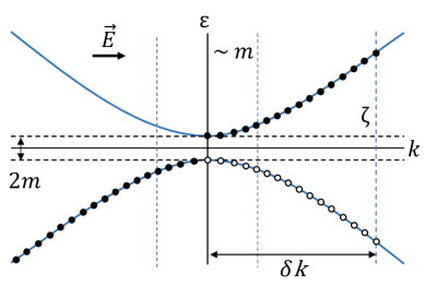
Figure 1: Illustration of the chiral anomaly in the Sine-Gordon model. The energy spectrum is sketched as two curves with an energy gap of $2m$, where $m$ is the soliton mass. In the presence of an $E$, solitons and antisoliton are generated and are shown by black dots in the top band and white dots in the bottom band, respectively. The range between two dashed lines in the middle corresponds to low-speed moving (anti)solitons. The minimum highest-level momentum of soliton pairs is labeled by $\zeta$.

To understand the role of the explicit chiral symmetry-breaking term, $V_{0}$, we consider the equation of motion

$$\partial_{t}j+u^{2}\partial_{x}\rho+2u^{2}\beta^{2}g\sin(2\sqrt{\pi}\Phi)=2u\beta^{2}\frac{eE}{\pi}$$ (22)

, where $j$ is given by Eq. 10 and the gap parameter $g\propto V_{0}$. This equation becomes equivalent to the gapless equation of motion Eq. 12 in the limit $V_{0}\rightarrow 0$. Furthermore, considering the excitations of the Sine-Gordon model shown in Fig. 1, where the gap is proportional to $m\sim g$, we see that the limit $m\sim g\rightarrow 0$ implies that almost all solitons and antisolitons move at the speed $u$. In this limit, the chiral charge is proportional to current $\rho_{c,sb}\simeq j/u$ (See detailed discussion in Appendix B). The chiral current is related to the chiral charge by the velocity of the modes so that $j_{c,sb}\simeq u\sum_{\sigma}[N_{\sigma s}+N_{\sigma\bar{s}}]\simeq u\rho$. Applying this to Eq. 22 (taking the limit $g\rightarrow 0$) leads to an anomaly equation

$$\partial_{t}\rho_{c,sb}+\partial_{x}j_{c,sb}=K\frac{eE}{\pi}.$$ (23)

This equation is essentially equivalent to the relativistic anomaly equation Eq. 12. Note that the role of the mass is rather subtle since we are using the limit $g\rightarrow 0$, which is the same limit considered in Eq. 12. However, the finite but vanishingly small $g$ is needed for the identification of $\rho_{c,sb}$ as a conserved chiral charge of solitons/antisolitions. This is because, as established earlier in the section one cannot identify this charge with left/right moving microscopic fermions. The latter identification is dependent on regularization. From an experimental standpoint, the validity of the above equation assumes an electric field that is applied over a relatively short time (i.e. relatively high frequency) relative to the mass $m\sim g$. The integrability of the Sine-Gordon model, which leads to the conservation of the chiral charge $\rho_{c,sb}$ and also remarkably the corresponding physical charge current $j$ allows one to measure the chiral charge at a later point to check the validity of the anomaly. As a matter of practice, one could simply measure the rescaled current $j/u$ as the chiral charge. This does not require an actual back-scattering potential. However, to check that this corresponds to a physical density, one would measure the soliton density at long times when the finite mass disperses the wave-packet so that individual solitons and antisolitons are separated. This check requires the backscattering $V_{0}$ to create the dispersion of the wave-packet and identify the individual charges.

III Momentum-based chiral charge and unrenormalized anomaly in 1D

The regularization issues described above can be resolved by defining a chiral charge density in terms of momentum density. To understand the idea behind using momentum density as a chiral charge density, let us first review how the mixed anomaly of translation symmetry and $U(1)$ symmetry is closely analogous to the chiral anomaly $U(1)$ Cho et al. (2017). In the low energy regime, we can expand the fermionic field operator $\psi(x,t)$ in a neighborhood of $\pm k_{F}$ according to the relation:

$${}\psi(x,t)\simeq e^{ik_{F}x}\psi_{R}(x,t)+e^{-ik_{F}x}\psi_{L}(x,t),$$ (24)

where $k_{F}$ is the Fermi momentum and the right and left fermionic fields $\psi_{R}$ and $\psi_{L}$ that are slowly varying in space and time. With the help of this preliminary step, the effect of a space translation transformation can be written as:

$$\left\{\begin{array}[]{l}{}\psi_{R}(x,t)\rightarrow\psi_{R}(x,t)^{\prime}=e^{ik_{F}a(x,t)}\psi_{R}(x,t)\\ \psi_{L}(x,t)\rightarrow\psi_{L}(x,t)^{\prime}=e^{-ik_{F}a(x,t)}\psi_{L}(x,t).\\ \end{array}\right.$$ (25)

Note that we ignore the shift of $\psi_{R/L}(x+a,t)$ by $a$ since these fields vary slowly compared to $k_{F}$. These transformations become equivalent to the chiral $U(1)$ transformation defined in Eq.(6) for $\beta(x)=k_{F}a(x)$.

While the total momentum displays properties of a chiral anomaly in systems with discrete translation symmetry Cho et al. (2017), systems with continuous translation symmetry allow us to study a local momentum density field, which is analogous to a chiral charge density. The chiral charge density is the Noether current associated with the chiral $U(1)$ symmetry in the systems described in Sec. II. Similarly one can identify the low energy limit of the canonical momentum density $T^{01}$, which is the Noether current associated with translation, as the analog chiral charge density for systems with finite bandwidth. However, unlike the anomalous chiral $U(1)$ symmetry, translation symmetry is preserved under quantization. Thus the momentum current density $T^{\mu 1}$ is conserved without any anomaly. Therefore the anomaly in this case is replaced by a mixed anomaly Cho et al. (2017) that arises from the gauge dependence of $T^{\mu 1}$ under the $U(1)$ symmetry associated with charge conservation. In the case of continuous translation symmetry, this mixed anomaly can be transformed into a chiral anomaly equation for a locally gauge-invariant analog of the momentum density as described below.

As a first example, we will start by computing the locally gauge-invariant momentum density, which we will call kinetic momentum density, to the 1DEG model. The action for the 1DEG model in the presence of an external gauge field in 1+1 is $S_{1DEG}=S_{2,0}+S_{2,int}$ with

$${}S_{2,0}=\int dxdt\,i\psi^{\dagger}D_{0}\psi-\frac{1}{2m}\bar{D}_{1}\psi^{\dagger}D_{1}\psi+\mu\psi^{\dagger}\psi,$$ (26)

where $D_{\mu}=\partial_{\mu}+ieA_{\mu}$ and $\mu$ is the chemical potential. For simplicity, we take the interacting part of the action as the density-density interaction with the form

$$S_{2,int}=\int dtdxdx^{\prime}V(x-x^{\prime})\rho(x)\rho(x^{\prime}),$$ (27)

where $\rho(x)=\psi^{\dagger}(x)\psi(x)$ is the fermion number density with $V(x-x^{\prime})$ being an interaction potential. As detailed in Appendix C, the stress-energy tensor, which is the Noether current associated with translation can be calculating by considering the variation of the action under translation following Eq. C. The spatial dependence of the vector potential $A_{\mu}(x,t)$ breaks translation-invariance and leads to a non-zero divergence of the stress-energy tensor

$$\partial_{\mu}T^{\mu\nu}=e\rho\partial^{\nu}A_{0}-ej\partial^{\nu}A_{1}$$ (28)

, where $\rho$ and $j$ are the charge density and current, respectively. The gauge dependence of $T^{\mu\nu}$ becomes apparent from the lack of gauge-invariance of the RHS of the divergence of $T^{\mu\nu}$. The gauge-invariance of the RHS can be restored by rewriting Eq. 28 as

$$\partial_{\mu}(T^{\mu\nu}-ej^{\mu}A^{\nu})=ej_{\mu}F^{\nu\mu}$$ (29)

, where the notation $F^{\nu\mu}$ represents the electromagnetic field tensor. The above equation motivates the definition of a kinetic stress-energy tensor $K^{\mu\nu}$ as

$$K^{\mu\nu}=T^{\mu\nu}-ej^{\mu}A^{\nu},$$ (30)

which has a gauge-invariant divergence

$$\partial_{\mu}K^{\mu\nu}=ej_{\mu}F^{\nu\mu}.$$ (31)

Using the calculated $T^{\mu\nu}$ in Appendix C, the kinetic momentum density $K^{01}$ and the kinetic stress $K^{11}$ are given by the manifestly gauge-invariant form

$$K^{01} = -i\psi^{\dagger}D_{1}\psi{}$$ (32)

$$K^{11} = i\psi^{\dagger}D_{0}\psi+\frac{1}{2m}\bar{D}_{1}\psi^{\dagger}D_{1}\psi$$ (33)

$$+\left[\int dx^{\prime}V(x-x^{\prime})\rho(x^{\prime})+\mu\right]\rho(x).$$

The electron gas model described by $S_{1DEG}$ is Galilean-invariant, which corresponds to the $uK=1$ case discussed in Sec. II.1, where the chiral charge is exactly equal to the current. Similarly, the chiral charge resulting from $K^{01}$ which will be discussed below is also equal to the current. At the same time, the spin-orbit coupled system discussed in Sec. II.1 requires higher derivative terms to describe. Therefore, we generalize the formalism to include higher spatial derivatives of the fermions with an action that is written as:

$$S_{h}=S_{1DEG}-\int dxdt\,V_{h}(\psi^{\dagger},\psi,D_{x}\psi,D_{x}^{2}\psi,\cdots).$$ (34)

Such an action can describe the spin-orbit coupled dispersion discussed in Sec. II.1 when only the lower band fermions are considered. The potential $V_{h}$ does not contain the time derivative term since Hamilton is assumed to be time-independent. The continuity equation of $K^{\mu\nu}$ is still Eq. 31, but $K^{\mu\nu}$ is modified to

$$K^{\mu\nu}\rightarrow K^{\mu\nu}+C^{\mu\nu},$$ (35)

where

$$C^{\mu\nu}=\frac{\partial V_{h}}{\partial(\partial_{\mu}A^{\rho})}\partial^{\nu}A^{\rho}\\ +\left[\frac{\partial V_{h}}{\partial(\partial_{\mu}\partial_{\rho}A^{\rho})}\partial^{\nu}\partial_{\rho}A^{\rho}-\partial_{\rho}\left(\frac{\partial V_{h}}{\partial(\partial_{\mu}\partial_{\rho}A^{\rho})}\right)\partial^{\nu}A^{\rho}\right]\\ +\cdots.$$ (36)

(See details in Appendix C)

As shown in Appendix C the kinetic momentum $K^{01}$ written Eq. 33 receives no corrections from the higher derivative corrections $V_{h}$, though the expression for $K^{11}$ is now more complicated. In addition, as detailed in Appendix C, kinetic stress-energy tensor $K^{\mu\nu}$ (Eq. 97) is gauge-invariant when the Lagrangian density is gauge-invariant and therefore can be used to define a gauge-invariant chiral charge.

Since $K^{01}$ has dimensions of momentum, one can convert the kinetic stress-energy tensor to a chiral current using the relation

$$j^{5\mu}:=K^{\mu 1}/k_{F}.$$ (37)

The corresponding momentum-based definition of the chiral charge density is

$$\rho_{c,mb}=K^{01}/k_{F}$$ (38)

This resolves the issue of identifying a nearly conserved chiral charge in a system without having to depend on regularization. The above result shows that in the systems of interest, the momentum density, which we know to be conserved in a system with continuous translation-invariance can be served as a conserved chiral charge. This is in contrast to the traditional chiral charge Eq. 9, which is only conserved in a TL model approximation, which requires a choice of regularization. Additionally, this definition is roughly consistent with Eq. 9 since for a weakly interacting system we expect the change in momentum $\delta T^{01}\sim k_{F}\rho_{c,cb}$. Finally, the conservation law for $j^{5,\mu}$ defined according to Eq. 37, which can be obtained from Eq. 31, is an anomaly equation that is identical to Eq. 16 that is written as:

$$\left<\partial_{\mu}j^{5\mu}\right>=\mathcal{A}_{5}=e\frac{n}{k_{F}}F^{10}=\frac{e}{\pi}E,$$ (39)

where we have simplified the RHS of Eq. 31 $\left<ej_{\mu}F^{1\mu}\right>=enE$. For the last equality we have used the Luttinger relation Luttinger (1960); Blagoev and Bedell (1997) $n=k_{F}/\pi$ is the average number density, and $E=F^{10}$ is the external electric field, which is the only non-zero component of the electromagnetic tensor in $1+1$D. This result is consistent with the non-Lorentz-invariant bosonization result in Eq. 16. In contrast to the Lorentz-invariant renormalized anomaly in Eq. 12, this anomaly is not renormalized by interaction. Note that the anomalous non-vanishing of the RHS of Eq. 39 in this case arises from the fact that $K^{1\mu}$ differs from $T^{1\mu}$, the conserved canonical stress-energy tensor, which is not gauge-invariant. This is thus the result of a mixed anomaly Cho et al. (2017) rather than the conventional chiral anomaly arising out of regularization.

IV Stability of Chiral anomaly in 3D

The chiral anomaly for non-interacting 3D systems can be understood Nielsen and Ninomiya (1983); Armitage et al. (2018) by focusing on the LL spectra in a magnetic field and applying the 1D results already discussed. However, this decoupling into 1D systems is not preserved in the presence of interactions. Additionally, as discussed in previous sections, the definition of chiral charge in 1D is ambiguous unless a momentum-based approach to chiral charge is used. On the other hand, 3D Weyl systems away from the Weyl point can be viewed as a topological Fermi liquid Haldane (2004) where the low energy response is described by free quasiparticles. The chiral charge associated with each Weyl point can be defined in terms of the Luttinger volume of each Fermi pocket without any reference to the regularization that was required in the 1D case. In Sec. IV.1, we generalize the momentum-based anomaly equation discussed in Sec. III to the 3D case. In Sec. IV.2, we show that this anomaly equation is equivalent to the anomaly equation based on the Luttinger-volume-based chiral charge. We contrast this, in Sec. IV.3 with the direct computation of the change in Luttinger volume using chiral kinetic theory Son and Spivak (2013). In Sec. IV.4, we describe how the momentum-based approach continues to apply in the low-temperature Landau level based limit beyond the application of chiral kinetic theory. Finally, in Sec. IV.5 we propose a pump-probe measurement of the Luttinger-volume-based chiral anomaly.

IV.1 Momentum anomaly in $3+1$D

For this section, we will assume that the separation between the Weyl points is small compared to the lattice constant so that the dispersion can be approximated by a continuum model Armitage et al. (2018) with conserved momentum. As will become clear in Sec. IV.4, while the lattice momentum in the $z-$direction is important to define the total momentum $P_{z}$ in the system, it does not play a role in the chiral anomaly. Additionally, the role of this lattice momentum can be eliminated (regularized) by defining the momentum relative to a trivial insulator that can be defined for the same model. The momentum-based chiral charge in 1+1D i.e. Eq. 37 can be generalized to 3+1D in a straightforward way as:

$${}j^{\mu,3D}_{c,mb}:=K^{\mu z}_{0}/k_{0}$$ (40)

, where $2k_{0}$ is the separation between the Weyl nodes and $K^{\mu z}_{0}$ are the kinetic stress-energy tensor associated with the electrons below the Weyl points. We choose the axes $z$ to be along the direction joining the two Weyl points. For the purposes of validity of Fermi liquid theory, we will assume that the Fermi level is away from the Weyl point. This means that $K^{\mu z}_{0}$ generically differs from $K^{\mu z}$, which is the kinetic stress tensor of the topological Fermi liquid Haldane (2004).

Following the kinetic momentum density approach to the chiral anomaly discussed in Sec. III for the 1D case, we start with the momentum conservation equation for a charged fluid (as in the $1+1$D case) in an electric field assuming the magnetic field along $z$-direction, i.e.

$$\partial_{0}\langle K^{0z}\rangle+\partial_{i}\langle K^{iz}\rangle=e\langle\rho\rangle E_{z}.$$ (41)

Note that the charge density $\rho$, unlike the 1D case is not related to $k_{0}$. In fact, the relevant part of the charge density $\rho$, here, is the contribution that is linear in $B$ because of the Streda relation:

$$\lim_{B\to 0}\left.\frac{\partial\rho_{e}}{\partial B}\right|_{\mu}=\frac{e^{2}}{4\pi^{2}}Q_{z}^{H}$$ (42)

, where $\rho_{e}=e\rho$, and $\sigma^{ab}_{H}(=(e^{2}/4\pi^{2})\epsilon^{abc}Q^{H}_{c})$ is the intrinsic Hall conductivity. As was shown by Haldane Haldane (2004), the vector $Q_{c}^{H}$ can be written as an integral over the Berry curvature over the Fermi surface

$$Q^{H}_{c}=\frac{1}{2\pi}\int d^{2}s[\nabla_{s}k_{p}\times\nabla_{s}k_{q}]_{s_{3}}\mathcal{F}_{pq}(k(s))k_{c}(s),$$ (43)

where the Berry curvature $\mathcal{F}_{pq}(k)$ is the Berry curvature on the Fermi surface and $\vec{s}$ parameterizes the Fermi surface. The anomalous Hall conductance is thus a well-defined property of a strongly interacting Fermi liquid.

The above relation also implies that for Weyl points with a net Berry flux, the vector $Q_{z}^{H}$ approaches $Q^{H}_{z}\rightarrow 2k_{0}$ in the limit of the Fermi energy approaching the Weyl point. When the Fermi energy is away from the Weyl point, one can apply the Streda relation Eq. 42 to the states between the Weyl point and the Fermi surface to calculate the magnetic field-induced correction to the charge density as

$$\delta\rho_{W}=\frac{e}{4\pi^{2}}\delta Q_{z}^{H}B=\frac{e}{4\pi^{2}}(Q^{H}_{z}-2k_{0})B.$$ (44)

Here $\delta\rho_{W}$ is the $B$-dependent correction to the extra density of electrons associated with the Fermi level being away from the Weyl point. This allows us to identify the electric field-induced change in momentum of the electrons between the Fermi surface and the Weyl point $K^{\mu z}_{0}$:

$$\partial_{\mu}(\langle K^{\mu z}-K^{\mu z}_{0}\rangle)=eE_{z}\delta\rho_{W}=\frac{e^{2}}{4\pi^{2}}E_{z}B\delta Q^{H}_{z}.$$ (45)

Subtracting this change from the total change in momentum (i.e. Eq. 41) and applying Eq. 42, we get

$$\partial_{0}\langle K^{0z}_{0}\rangle+\partial_{i}\langle K^{iz}_{0}\rangle=\frac{e^{2}}{2\pi^{2}}k_{0}E_{z}B.$$ (46)

Combining this observation with the definition of chiral charge Eq. 40 leads to the chiral anomaly equation

$$\partial_{0}\langle\rho^{3D}_{c,mb}\rangle+\partial_{i}\langle j^{i,3D}_{c,mb}\rangle=\frac{e^{2}}{2\pi^{2}}(\boldsymbol{E}\cdot\boldsymbol{B})$$ (47)

We note that we have not explicitly written an expression for the chiral current $K^{iz}_{0}$ since it is not necessary to define the chiral anomaly coefficient. But this is expected to be a direct generalization of Eq. 46. We also note that this momentum-based chiral anomaly is unrenormalized as expected though the momentum $K^{0z}_{0}$ and $k_{0}$ individually might be renormalized by interactions.

The inclusion of Coulomb interactions between the electrons, in the absence of other trivial Fermi surfaces, constrains the total electron density of the bulk 3D system to be constant instead of the constant chemical potential assumed so far. This results in a correction to the chemical potential in response to the magnetic field $B$ because of the Streda relation

$$\delta\mu_{B}=-\frac{e^{2}}{4\pi^{2}}Q_{z}^{H}B/N(0),$$ (48)

since the spectral flow induced change in charge density at constant chemical potential (i.e. Eq. 42) is compensated by $\delta\mu_{B}$. This magnetic field-induced change in chemical potential is by itself an interesting variant of the chiral anomaly since this is another way how the electromagnetic field can affect the total charge of the Weyl point. As a result of this change, Eq. 44 for the charge density around the Weyl point is modified to

$$\delta\rho_{W}^{(Coul.)}=\frac{eB}{4\pi^{2}}\left(\delta Q_{z}^{H}+N(0)\delta\mu_{B}\right)=-\frac{eB}{2\pi^{2}}k_{0}$$ (49)

Interestingly, the charge neutrality constraint implies that $\rho$ in Eq. 41 must vanish. Despite this, the application of Eq. 45 leads to the conclusion that the chiral anomaly equation Eq. 47 is preserved even when the charge neutrality limit is enforced by Coulomb interactions. This is one rather stringent test of the robustness of the anomaly to interactions.

IV.2 Luttinger Volume-based Chiral Charge

The electric field $E$ typically changes the momentum of the quasiparticles at the Fermi surface by shifting the Fermi surface resulting in a momentum contribution $eE_{z}\delta\rho_{W}$. But, as seen from Eq. 45, the change in the Weyl part of the momentum $K^{0z}_{0}$ explicitly excludes this piece. Therefore, the change $\delta K^{0z}_{0}$ must arise from an electric field induced transfer of charge between the two Weyl points that are separated by the wave-vector $2k_{0}$ so that $k_{0}^{-1}\delta K^{0z}_{0}=\delta\rho^{3D}_{c,mb}=\delta\rho_{w}$ is the number of electrons transferred between the Weyl points. Such a transfer of charge between the Weyl points has also been derived using chiral kinetic theory  Stephanov and Yin (2012); Son and Spivak (2013); Haldane (2004) and is explicitly written as:

$$\frac{\partial\rho_{w}}{\partial t}+\nabla\cdot\boldsymbol{j}^{3D}_{c,FS}=\frac{e^{2}}{2\pi^{2}}(\boldsymbol{E}\cdot\boldsymbol{B})$$ (50)

in the low-temperature limit, in which scatterings between two Weyl nodes can be suppressed and neglected. In fact, this non-conservation of the Weyl point charge $\rho_{w}$ is the original definition of the chiral anomaly in $3+1$D Adler and Bardeen (1969), which however requires regularization. However, in the finite electron density limit discussed here, this chiral charge at the Weyl points $\rho_{w}$, which is equivalent to the momentum-based chiral charge $\rho^{3D}_{c,mb}\equiv\rho_{w}$, can be defined as a Fermi-surface property through the Luttinger volume as:

$${}\rho^{3D}_{c,FS}\equiv\rho_{w}:=\sum_{\alpha=\pm}\gamma_{\alpha}\int_{\overline{FS}_{\alpha}}\frac{d^{3}k}{(2\pi)^{3}}$$ (51)

, where $FS_{\alpha}$ represents the separate Fermi surfaces around two Weyl nodes, and $\gamma_{\alpha}=\pm$ indicates the chirality of the Weyl nodes. Eq. 51 represents a form of chiral charge, that is well-defined even for interacting systems where Fermi surfaces are defined as $G^{-1}(k,\omega=0,\mu)=0$, where $G$ is the single-particle Green’s function. The Luttinger volume provides an interaction robust definition of a chiral charge that does not rely on any form of regularization that is not available in $1+1$D or in the strong magnetic field limit with only the chiral Landau level being occupied where the chiral anomaly is often discussed Nielsen and Ninomiya (1983).

It should be noted that the equivalence of the momentum-based chiral anomaly $\rho^{3D}_{c,mb}$ and the chiral charge $\rho_{w}$ breaks down when the Fermi surface is at finite temperature and sufficiently far from the Weyl point. This is because at finite temperature $T$, the scattering of quasiparticles around the Fermi surface which conserve momentum but not chiral charge as shown in Fig.2 will contribute to relaxation of the chiral charge $\rho_{w}$ at rate $\sim T^{2}$. However, such scatterings have no influence on the total momentum; the momentum-based chiral anomaly provides immunity against scattering.

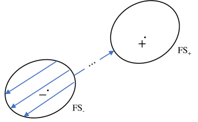
Figure 2: Schematic of a scattering pattern around the Fermi surface at finite $T$.

The rates of such relaxation will be highly suppressed at any finite temperature since this will have to be a very correlated multiparticle process. On the other hand, momentum can be affected even by intra-Weyl node disorder scattering which does not affect $\rho_{w}$. In the case of discrete translation symmetry, Umklapp scatterings from the lattice will eliminate the momentum-based chiral anomaly. The rates of such relaxation processes are expected to be suppressed in the low-density limit where the Weyl points are close to each other relative to the Brillouin zone.

IV.3 Chiral kinetic theory

The results of the arguments in Secs. IV.1 and  IV.2 can be checked explicitly using chiral kinetic theory of the quasiparticles Son and Yamamoto (2012) of the topological Fermi liquid Haldane (2004). This is valid in the limit that the magnetic field is small enough so that the associated cyclotron frequency is much below the thermal energy, i.e., $\omega_{B}\ll k_{B}T$. In the Fermi liquid limit, this chiral kinetic theory has been successfully used to understand the properties of topological Fermi liquids Stephanov and Yin (2012); Duval et al. (2006); Son and Spivak (2013); Xiao et al. (2005). Below we will use it to validate the properties of the momentum-based chiral charge as well as the measured chiral charge discussed in Secs. IV.1 and  IV.2.

The central equation of kinetic theory is the Boltzmann equation:

$$\frac{\partial f}{\partial t}+\frac{\partial f}{\partial\boldsymbol{r}}\cdot\dot{\boldsymbol{r}}+\frac{\partial f}{\partial\boldsymbol{k}}\cdot\dot{\boldsymbol{k}}=I_{coll}=-\frac{\delta f}{\tau}$$ (52)

, where $f=f(\boldsymbol{r},\boldsymbol{k},t)$ is the quasiparticle distribution function. The quasiparticles can only change their state and be equilibrated through collisions, which are approximated by the relaxation time approximation with a constant collision frequency $1/\tau$.

The equations of motion for quasiparticles in the presence of an anomalous velocity Karplus and Luttinger (1954) is written as:

$$\dot{\boldsymbol{k}} = e\boldsymbol{E}+e\dot{\boldsymbol{r}}\times\boldsymbol{B}$$ (53)

$$\dot{\boldsymbol{r}} = \boldsymbol{v_{k}}+\dot{\boldsymbol{k}}\times\boldsymbol{\Omega}_{\boldsymbol{k}}$$ (54)

, where $A_{\boldsymbol{k}}=i\left<u_{\boldsymbol{k}}|\nabla u_{\boldsymbol{k}}\right>$, $\boldsymbol{\Omega}_{\boldsymbol{k}}=\nabla\times A_{\boldsymbol{k}}$ is the Berry curvature, and the group velocity $\boldsymbol{v_{k}}=\nabla_{k}\varepsilon$. Due to the Berry curvature term in the above equations leads to a violation of Liouville’s theorem by the RHS of Eq. 52  Xiao et al. (2005) This can be rectified by introducing a phase space density factor $G_{\boldsymbol{k}}=(1+e\boldsymbol{B}\cdot\boldsymbol{\Omega}_{\boldsymbol{k}})^{2}$, which satisfies an equation of motionStephanov and Yin (2012)

$$\frac{\partial}{\partial t}\sqrt{G_{k}}+\frac{\partial}{\partial\boldsymbol{r}}\cdot(\sqrt{G_{k}}\dot{\boldsymbol{r}})+\frac{\partial}{\partial\boldsymbol{k}}\cdot(\sqrt{G_{k}}\dot{\boldsymbol{k}})=e^{2}(\boldsymbol{E}\cdot\boldsymbol{B})\nabla\cdot\boldsymbol{\Omega}_{\boldsymbol{k}}.$$ (55)

We can define a conserved phase-space density $\tilde{f}=\sqrt{G_{k}}f$ that obeys Liouville’s theorem by combining the phase-space density $\sqrt{G_{k}}$ with the distribution function $f$, which now obeys the conservation law

$$\frac{\partial}{\partial t}\tilde{f}+\frac{\partial}{\partial\boldsymbol{r}}\cdot(\tilde{f}\dot{\boldsymbol{r}})+\frac{\partial}{\partial\boldsymbol{k}}\cdot(\tilde{f}\dot{\boldsymbol{k}})=e^{2}(\boldsymbol{E}\cdot\boldsymbol{B})\nabla\cdot\boldsymbol{\Omega}_{\boldsymbol{k}}f+\tilde{I}_{coll}$$ (56)

, where $\tilde{I}_{coll}=\sqrt{G_{k}}I_{coll}$. Using the above equation of motion for the phase space density $\tilde{f}$, we can find the continuity equation for the Luttinger volume-based chiral charge in Sec.IV.2 and the kinetic momentum

$$\boldsymbol{P}=\int_{\boldsymbol{k}}\boldsymbol{k}\tilde{f}$$ (57)

in Sec.IV.1. The result of the first one (Eq.50) has been already discussed in many references and Sec.IV.2. The second one, regarding the kinetic momentum, is written as

$${}\frac{\partial}{\partial t}\boldsymbol{P}+\nabla\cdot\vec{\boldsymbol{K}}=\frac{e^{2}}{4\pi^{2}}(\boldsymbol{E}\cdot\boldsymbol{B})\boldsymbol{Q}^{H}+\int_{\boldsymbol{k}}(e\boldsymbol{E}+e\boldsymbol{v_{k}}\times\boldsymbol{B})f.$$ (58)

, where

$$\vec{\boldsymbol{K}}=\int_{\boldsymbol{k}}\left(\boldsymbol{v_{k}}+e\boldsymbol{E}\times\boldsymbol{\Omega}_{\boldsymbol{k}}+e\left(\boldsymbol{v_{k}}\cdot\boldsymbol{\Omega}_{\boldsymbol{k}}\right)\boldsymbol{B}\right)\boldsymbol{k}f$$ (59)

, a dyadic tensor, is the stress tensor, and

$$\boldsymbol{Q}^{H}=4\pi^{2}\int_{\boldsymbol{k}}\boldsymbol{\Omega}_{\boldsymbol{k}}f=\sum_{\alpha}\boldsymbol{Q}^{H}_{\alpha}=\frac{1}{2\pi}\sum_{\alpha}\int_{S_{\alpha}}d^{2}\mathcal{F}\,\boldsymbol{k}$$ (60)

, which is just the vector associated with the AQH conductivity in the Streda formula Eq.42. The collision term will not contribute if we assume collisions are elastic. Incidentally, this equation is general for any condensed matter system, and interactions will not be affected.

To obtain the momentum-based chiral anomaly equation from Sec.IV.1, we still consider the $z$-direction component of the kinetic stress-energy tensor and assume the magnetic field also along $z$. Eq.58 will be simplified:

$$\frac{\partial}{\partial t}P^{z}+\nabla\cdot\vec{K}^{z}=\frac{e^{2}}{2\pi^{2}}(\boldsymbol{E}\cdot\boldsymbol{B})Q^{H}_{z}.$$ (61)

Restricting the integrals in Eqs. 57 and  60 to above the Weyl point leads to a variation of the above equation:

$$\frac{\partial}{\partial t}(P^{z}-P^{z}_{0})+\nabla\cdot(\vec{K}^{z}-\vec{K}^{z}_{0})=\frac{e^{2}}{2\pi^{2}}(\boldsymbol{E}\cdot\boldsymbol{B})\delta Q^{H}_{z},$$ (62)

where $P^{z}$ and $Q^{H}_{z}$ are replaced by $(P^{z}-P^{z}_{0})$ and $\delta Q^{H}_{z}=Q_{z}^{H}-2k_{0}$, which are the momentum and anomalous Hall contributions of electrons above the Weyl point, respectively. Not that $P^{z}_{0}$ and $2k_{0}$ are the intrinsic momenta and the anomalous Hall contributions of the Weyl point. This provides a more quantitative understanding of Eq. 45 from Sec. IV.1. By combining Eq. 61 with Eq. 62 leads us back to the chiral anomaly equation:

$${}\frac{\partial}{\partial t}P_{0}^{z}/k_{0}+\nabla\cdot\vec{K}_{0}^{z}/k_{0}=\frac{e^{2}}{2\pi^{2}}(\boldsymbol{E}\cdot\boldsymbol{B}),$$ (63)

Thus, the analysis of the contribution of the Weyl point to the momenta $P^{z}_{0}$ provides a more microscopic derivation (i.e. in terms of FL quasiparticles) of the anomaly equation Eq. 47.

As a side, the chiral kinetic theory can also compute the chiral magnetic effect(CME). The current along $B$-direction can be written asStephanov and Yin (2012)

$$\boldsymbol{j}_{\rm{CME}}=e^{2}\boldsymbol{B}\int_{\boldsymbol{k}}f\left(\boldsymbol{v_{k}}\cdot\boldsymbol{\Omega}_{\boldsymbol{k}}\right)=\frac{e^{2}\boldsymbol{B}}{4\pi^{2}}\Delta\mu,$$ (64)

where

$$\Delta\mu=\frac{1}{2\pi}\sum_{\alpha}\int_{S_{\alpha}}d^{2}\mathcal{F}\,\varepsilon(\boldsymbol{k})$$ (65)

(See details in Appendix D). If we assume that the electron distribution functions have equilibrium forms in the individual valleys, $\Delta\mu$ is exactly the chemical potential difference at the Fermi level and Eq.64 consistent with referencesSon and Spivak (2013); Armitage et al. (2018). Eq.64 is robust since it only depends on Fermi surfaces. Hence, the conductivity along the magnetic field direction, $\sigma_{zz}$, is modified asSon and Spivak (2013); Armitage et al. (2018)

$$\sigma_{zz}(B)=\sigma_{zz}(0)+\frac{e^{4}B^{2}\tau_{a}}{4\pi^{4}g(\epsilon_{F})}$$ (66)

, where $g(\epsilon_{F})$ is the density of state and $\tau_{a}$ is the inter-nodes scattering time.

IV.4 Low Temperature Landau Level Limit

IV.4.1 Model

The discussion so far has assumed a temperature that is high relative to the small applied magnetic field. However, all the conclusions go through equally well at nearly zero temperature. The low temperature for a non-interacting Weyl system in a magnetic field is described by the chiral Landau level Nielsen and Ninomiya (1983). To illustrate this, we will compute the non-interacting Landau levels for the continuum Weyl toy model  Armitage et al. (2018), which is written as:

$$H_{wl} =H_{0}+H_{R}$$ (67)

$$=(k^{2}-k_{0}^{2})\sigma_{z}+v(k_{y}\sigma_{x}-k_{x}\sigma_{y})$$

, where $k^{2}=k_{x}^{2}+k_{y}^{2}+k_{z}^{2}$ and $v$ is the Rashba coupling constant. The energy spectrum is indeed the Weyl type in the low energy regime, which has two touching Weyl points at $\boldsymbol{k}=(0,0,\pm k_{0})$ when $v\neq 0$.

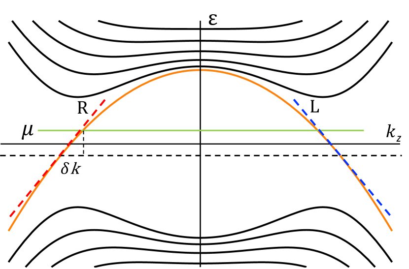
Figure 3: Band structure of Weyl model ($k_{0}=1$) in the Sec.IV.4 with a small spin-obit coupling $v=1.5$ under the magnetic field $B=0.1$. The chemical potentials are set away from the Weyl nodes, and the low energy states are basically multiply LLs.

To study the chiral anomaly, when applying the magnetic field $B$ along the $z$-direction, we calculate the LL spectrum of the Hamiltonian $H_{wl}$ in the presence of a magnetic field as shown in Fig. 3. While the magnetic field preserves angular momentum, the spin-orbit coupling mixes the $(\sigma_{z}=1,n)$ and $(\sigma_{z}=-1,n+1)$ (where $n$ labels the conventional Landau levels without spin-orbit) and opens a gap in the spectrum. However, one of the Landau levels $(\sigma_{z}=-1,n=0)$ does not have a partner to hybridize and remains gapless. This Landau level, which is referred to as the chiral Landau level, is responsible for the chiral anomaly in an applied electric field within the non-interacting limit Nielsen and Ninomiya (1983). Note that the gap in the non-chiral LLs in Fig. 3 actually occurs at negative energies as opposed to the previous calculation of LL spectra of individual Weyl cones Nielsen and Ninomiya (1983); Armitage et al. (2018); Burkov (2018). This difference is a manifestation of the Streda formula i.e. Eq. 42, which as discussed in Sec. IV.1 is critical for understanding the chiral anomaly from a momentum conservation perspective.

IV.4.2 Momentum-based anomaly

The chiral anomaly is conventionally defined, using the argument of Nielsen and Ninomiya Nielsen and Ninomiya (1983), as non-conservation of chiral charge can be determined from the LL spectrum in Fig. 3 for the non-interacting case where the chemical potential is in the gap of the non-chiral LLs. This argument also leads to a current that appears to be renormalized by interactions Rylands et al. (2021), which, similar to the $1+1$D results discussed in Sec. II, depends on the regularization scheme used for the calculation.

However, the subtleties of defining chiral charge discussed in Sec. II arise when only the Fermi level intersects just the chiral LL, and therefore the other LLs are important in defining chiral charge. Therefore, it is beneficial to consider the chiral anomaly away from the Weyl points, where several non-chiral LLs are also occupied. These non-chiral LLs do not contribute to the change in chiral charge in response to an electric field and therefore do not modify the chiral anomaly Armitage et al. (2018). These non-chiral LLs do, however, affect the momentum-based definition of chiral charge since they contribute to momentum change under an electric field. This turns out to not be a problem because similar to the case discussed in Sec. IV.1, the contribution of non-chiral LLs as well as the electrons in the chiral LL above the Weyl point to the change in momentum can be calculated directly from the density of electrons in the respective LLs. For small magnetic fields corresponding to $\omega_{B}\ll E_{F}$, this density is given by the FS volume. Subtracting the momentum contribution of electrons above the gap of the non-chiral LLs leaves only the momentum contribution associated with a transfer of electrons from one Weyl point to the other. This can be estimated to be $2k_{0}(B/2\pi)(E_{z}\delta t)$ where $E_{z}\delta t$ is the change in momentum of the electrons and $B/2\pi$ is the degeneracy per unit area of the chiral Landau level. The factor $2k_{0}$ arises from the length of the unoccupied segment (or occupied by holes) of the chiral Landau level in Fig. 3. Since $2k_{0}$ is the distance between the Fermi points on the chiral LL when the chiral LL crosses the gap of the non-chiral LL, the momentum density can be interpreted as a chiral charge that is consistent with the result Eq. 47. The chiral LL in Fig. 3 leaves an ambiguity in the value of $2k_{0}$ to be in a range where the chiral LL crosses the gap. This ambiguity drops out in the limit of small $B$ since the gap also vanishes in this limit.

Fully filled LLs (including a fully filled chiral Landau level) will not contribute to the continuity equation Eq. 41. This is because the total crystalline momentum along $k_{z}$ generated by a slowly time-varying external electric field $E_{z}$ that increases a vector potential $\delta A_{z}=E_{z}\delta T=\Phi_{0}/L_{z}$, changes the momentum on the r.h.s of Eq.41 by a primitive reciprocal lattice vector. Note that the lattice does play an essential role in regularizing the otherwise divergent momentum. However, one would obtain the same result from other regularizations such as by considering the difference in momentum between this chiral system and a variant of Rq. 67 with a trivial gap generated by a $\sigma_{x}$ term instead of the spin-orbit term.

IV.4.3 Interaction effects

The effect of interactions can be included in a Fermi liquid theory in this framework if one goes away from the Weyl point (relative to the cyclotron frequency) i.e. $E_{F}\gg\omega_{B}$. In this limit and in the presence of a small magnetic field $\boldsymbol{B}=B\hat{\boldsymbol{n}}$, the quasiparticles near the FS follow semiclassical orbits (given by Eq. 54 with $\vec{E}=0$) which are confined to planes with constant parallel momentum $\vec{k}\cdot\hat{n}=k$, with a long scattering lifetime. The Fermi-surface orbit in $k$-space on the FS labelled by $\alpha$, has a cross-sectional area $A_{\alpha}(k)$ that is set by a quantization condition Ashcroft and Mermin (2022)

$$A_{\alpha}(k^{n}_{F\alpha})l_{B}^{2}-\phi_{\alpha}(k^{n}_{F\alpha})=2\pi(n+\frac{1}{2}),$$ (68)

where $l_{B}^{2}=1/eB$, and $n$ is an integer that labels the Landau orbits (i.e. bands in Fig. 3) and $\phi_{\alpha}(k)$ is the Berry phase of the quasiparticle on the phase-space orbit at $\vec{k}\cdot\hat{n}=k$ on $FS_{\alpha}$. The Landau band in Fig. 3 with an extremum closest to the Fermi level represents the pair of Landau orbits on the FS that is closest to the maximum area orbit at $k=k_{max}$ of the FS. These are the orbits that contribute to quantum oscillations that are used to determine the size of the Fermi surface Ashcroft and Mermin (2022). The solution with the maximum $|k|$ is the chiral Landau level, which is a result of the difference in Berry phase $2\pi c_{\alpha}=\phi_{\alpha}(k_{1})-\phi_{\alpha}(k_{2})$, where $k_{1}>k_{max}>k_{2}$ represent the range of $k$ of the $FS_{\alpha}$ and $c_{\alpha}=\pm 1$ is the Chern number of Fermi surface around Weyl point $\alpha$. The resulting LL spectrum near the FS is essentially identical to the non-interacting one seen in Fig. 3, except that the energy spectrum away from the Fermi energy is ill-defined because of the imaginary part of the self-energy. The response to an external electric field $\boldsymbol{E}$ in the time period $\delta t$ is determined by the states near the Fermi energy, which is therefore identical to the non-interacting case discussed in the previous paragraph and is described by Eq. 47.

IV.5 Measuring the Luttinger-volume-based chiral anomaly

The quantum oscillations that arise from the extremal Landau bands at $k=k_{max}$ discussed in the previous subsection can in principle be used to detect the Luttinger-volume-based chiral anomaly discussed in Sec. IV.2 by measuring the chiral charge transfer in a pump-probe measurement. The central idea is to use quantum oscillations to measure the anomaly-induced change in Fermi wave-vector as is done in magneto-transport (i.e. the Shubnikov-de Hass effect) Ashcroft and Mermin (2022). This effect relies on the fact that the low-frequency longitudinal conductivity would show dips associated with peaks in the density of states (DOS) when the Fermi level crosses a band extremum in Fig. 3. This corresponds to an extremal LL becoming allowed on the FS. For simplicity we will assume that the Fermi surface is nearly spherical near the Weyl point so that the electron number density in Weyl point $\alpha$, $N_{\alpha}=A_{\alpha}(k_{max})^{3/2}/6\pi^{7/2}$, can be written in terms of the extremal area $A_{\alpha}(k_{max})$.

Our protocol to measure the Luttinger-volume-based chiral anomaly discussed in Sec. IV.2 consists of three steps.

Step (1): Choose a magnetic field $B$ so that the FS quasiparticle DOS is at a local maximum as evident from a minimum in the measured longitudinal conductance. In our model, this corresponds to $k_{max}$ satisfying Eq. 68 for an integer $n$.

Step (2): Apply a ”pump” electric field $E_{z}$ for a short time $\delta t$ and wait for a relaxation time $\tau$.

Step (3): Measure the longitudinal conductance using a ”probe” field to see if the conductance is near the minimum value. Repeat step (2) with a different $\delta t$ till one reaches near the minimum value. The result of the measurement is $\Lambda=eE_{z}\delta T$ that transfers the system from one conductance minimum to another.

For small magnetic field $B$, the change $\delta k$ in $k_{max}$ is insignificant so that we can ignore the Berry phase term and simplify Eq. 68 to $\delta A_{\alpha}=2\pi\alpha eB$. The corresponding change in number density is $\delta N_{\alpha}=4\alpha A_{\alpha}(k_{max})\delta k/(2\pi)^{3}=eB\alpha\sqrt{A_{\alpha}(k_{max})}/2\pi^{5/2}$. Assuming an unrenormalized chiral anomaly and using Eq.50, the predicted $\Lambda$ would be

$$\Lambda_{predict}=eE_{z}\delta T=\frac{2\pi^{2}}{e}\frac{\delta(N_{+}-N_{-})}{B}=2\sqrt{\frac{A_{\alpha}(k_{max})}{\pi}}.$$ (69)

The measured value of $\Lambda$ determines the Luttinger-volume-based chiral charge transfer between the two Fermi surfaces, which based on results in this section should not be renormalized by interactions or other complexities of the system.

V Summary and Discussion

In summary, we start by illustrating the difficulties of applying chiral anomaly calculations from relativistic field theories by comparing the results to that from Hamiltonian bosonization in Sec. II. We show that these ambiguities in the chiral anomaly equation are resolved by replacing the chiral anomaly by mixed anomaly between the translation and $U(1)$ charge symmetry Cho et al. (2017). The chiral anomaly equation here is qualitatively consistent with the corresponding effective action term derived previously using the correspondence between the t’Hooft and mixed anomalies Wang et al. (2021). We find that the mixed anomaly approach in $1+1$D leads to a chiral charge which is defined as the kinetic momentum divided by the Fermi wave vector $k_{0}$. The electromagnetic force term in the kinetic stress-energy continuity equation corresponds to the anomalous i.e. chiral symmetry breaking term. The resulting chiral anomaly equation is unrenormalized by interactions. We find it is still possible to realize an interaction renormalized Lorentz-invariant anomaly in Luttinger liquids with weak backscattering. Such systems can be approximated by Sine-Gordon models. The chiral charge in this case must be chosen to be a fermionic representation based on solitons and antisolitons.

We then apply the mixed anomaly technique Cho et al. (2017) to $(3+1)$D Weyl systems. Similar to previous work mapping the t’Hooft anomaly to an effective action term in a mixed anomaly representation Wang et al. (2021), we can use the Streda formula to show that the anomaly based on the difference of charge density around Weyl pockets is robust and unrenormalized. This is quite different from the chiral magnetic effect Armitage et al. (2018), whose manifestations appear with various non-universal prefactors that are renormalized by interactions. While some of these prefactors such as density of states or Fermi velocity may be determined from other measurements, it is unclear whether the chiral magnetic effect is the only contributor to these currents. As an example of such subtleties, we note that the homogeneous finite frequency Hall conductivity $\sigma_{xy}(\omega)$ of a Weyl material Rylands et al. (2021) was found, using heat Kernel regularization, to contain a second-order term ($O(\omega^{2})$) that was entirely determined by interaction strength. On the other hand, a numerical calculation of the ac Hall conductivity in a non-interacting model of a Weyl material shows a non-zero and non-universal second-order term even in the absence of interactions (See Appendix E). Similarly, a direct interpretation of the chiral magnetic effect in terms of the axion term in the effective action Chen et al. (2013); Goswami and Tewari (2013) suggests a magnetic field-induced current at a finite magnetic field. While such response terms can occur for finite frequency magnetic fields with open boundary conditions Alavirad and Sau (2016) as well as in the form of the gyrotropic magnetic effect Ma and Pesin (2015); Zhong et al. (2016), this response is not observable in the presence of any physical equilibriation Vazifeh and Franz (2013). To avoid these subtleties, we focus on the violation of charge conservation in an individual Weyl pocket as the robust signature of the chiral anomaly in Weyl semimetals. This observable in $(3+1)D$ does not survive the ambiguities in $(1+1)D$ and can be defined in terms of the Luttinger volume of the topological Fermi surface Haldane (2004). While this is substantially more difficult to measure than a current response, we propose a rather experimentally intricate pump-probe measurement to directly measure the changes in the Luttinger volume in response to an electromagnetic field.

It should be noted that, in contrast to prior work Cho et al. (2017); Wang et al. (2021), to derive the chiral anomaly equations of motion we consider a mixed anomaly between $U(1)$ charge and continuous space translation. This leads to us having to use a regularization for the kinetic momentum discussed in Sec. IV.4.2 where we subtract off the contribution of the closest gapped insulator. This only makes sense if the Weyl points are close in momentum space relative to the total Brillouin zone as in the model described in Sec. IV.4. This is quite different from the Chern insulator stack model of a Weyl semimetal Armitage et al. (2018) and the approach to the anomaly considered here may not apply to that case. On the other hand, the chiral kinetic theory Son and Yamamoto (2012) for the charge density of each pocket would still imply a quantized change in chiral charge, thus predicting a robust chiral anomaly. However, this relies on the full Fermi liquid emergent IR symmetry of conservation of quasiparticles Else et al. (2021). This would be broken at finite temperature scattering of quasiparticles and Umklapp scattering from the edge of the Brillouin zone can eliminate the conservation of chiral charge. The continuum case considered here is more robust because the anomaly fundamentally is defined in terms of a continuum momentum that is conserved in a ”low density” limit. Of course, disorder scattering  Armitage et al. (2018) complicates this entire discussion and there cannot be a precisely defined notion of chiral anomaly in this case. The realistic definition of the chiral anomaly necessarily requires considering appropriate assumptions about the scaling with disorder Son and Spivak (2013); Burkov (2015); Armitage et al. (2018).

The definition of the anomaly in this work has been in terms of the equations of motion similar to the original works Adler (1969); Bell and Jackiw (1963); Georgi and Rawls (1971) rather than the effective action approach for the t’Hooft anomaly of the emergent IR chiral symmetry Else et al. (2021). In fact, the topological chiral anomaly terms in the effective action from a microscopic mixed anomaly of $U(1)$ gauge and translation have already been worked out Wang et al. (2021). This approach is more general compared to the results presented here because it allows a general translation of known t’Hooft anomalies of various low-energy theories to mixed-anomaly-based responses in an effective action. In the context of Weyl, this work Wang et al. (2021) clearly shows signatures of the chiral Landau level and presumably other features of the chiral anomaly. In contrast, the present work only presents the equation of motion responses of the chiral anomaly, which are sometimes subtle to extract from an effective action as has been discussed in the previous paragraph. A direct approach for deriving the universal aspects of the microscopic response function from the effective action Wang et al. (2021) would be an interesting future direction that would provide a general anomaly formalism applicable to condensed matter systems.

Appendix A Details of Bosonization

A.1 Lorentz-invariance Constrained Chiral Anomaly

Let us now review the chiral anomaly in the relativistic case where we have chosen $\lambda_{\mu\nu}^{(2)}=\lambda\eta_{\mu\nu}$ so that $S_{LL}$ is then the Lorentz-invariant Thirring model Georgi and Rawls (1971). In this case, the collective mode velocity $u$ continues to match the Fermi velocity $u=v_{F}=1$, and current and density have the same units. The chiral anomaly equation for this so-called Thirring modelGeorgi and Rawls (1971), which was derived using perturbation theory together with a Lorentz-invariant regulator, shows a renormalization. Here we use bosonization to derive the anomaly equation in a way where Lorentz and non-Lorentz-invariant results can directly be compared.

We consider the Euclidean (i.e. Wick rotated) space-time Stone (1994) so that the point-splitting expansion is manifestly rotation (i.e. Lorentz)-invariant in the Wick rotated $(1+1)$D plane. Using this scheme of normal ordering the chiral fermionic operators $\psi_{R,L}(x,t)$ can be written as vertex operators of chiral bosonic operators $\Phi_{R,L}(x,t)$, which in turn can be used to define the bosonic field $\Phi(x,t)$ Stone (1994). Applying the standard bosonization identities in Euclidean space Stone (1994) for replacing the Fermions in the kinetic term, $S_{1,0}$, we obtain

$$S_{1,0}=\frac{1}{2K}\int(\partial_{\mu}\Phi)^{2}$$ (70)

, where $x_{0}=t$ and $K=1$. Similar use of the bosonization identities Stone (1994) leads to related expressions for the chiral current and the $U(1)$ charge current, which can be written as

$$j^{\mu}=\frac{1}{\sqrt{\pi}}\epsilon^{\mu\nu}\partial_{\nu}\Phi\,\quad j^{5\mu}=\frac{1}{\sqrt{\pi}}\partial^{\mu}\Phi,$$ (71)

where $\epsilon^{\mu\nu}$ is the completely anti-symmetric unit tensor.

Applying these identities to $S_{1,int}$ leads to an additional contribution to Eq. 70, so that the $K$ factor depends on the interaction strength in the fermionic model as

$$K^{-1}=1+\lambda/\pi,$$ (72)

where $\lambda=g_{2}$ and $g_{4}=0$ because of Lorentz-invariance.

The coupling to an external vector potential $A_{\mu}$ is included through a term

$$\mathcal{L}_{em}=-ej^{\mu}A_{\mu}=-\frac{e}{\sqrt{\pi}}A_{\mu}\epsilon^{\mu\nu}\partial_{\nu}\Phi.$$ (73)

While the charge current $j^{\mu}$ in Eq. 71 is manifestly conserved, the divergence of the chiral current can be written in terms of the classical equation of motion for $\Phi$ as

$${}\mathcal{A}^{Tr}_{5}=\left<\partial_{\mu}j^{5\mu}\right>=\partial_{\mu}\partial^{\mu}\Phi/\sqrt{\pi}=\frac{1}{1+\lambda/\pi}\frac{e}{\pi}E.$$ (74)

where $E=\partial_{0}A_{1}-\partial_{1}A_{0}$ is the electric field. This result is obtained by using the expression for the chiral current Eq. 71 and then combining with Eq. 70 with Eq. 73. This shows that the chiral charge, in contrast to the classical result is not conserved since the right-hand side is non-zero and is proportional to the electric field $E$. This is referred to as the chiral anomaly equation. Furthermore, since the right hand side depends on the interaction strength $\lambda$, the chiral anomaly is renormalized by interactionGeorgi and Rawls (1971). This result is identical to that obtained directly from the Thirring model using either Pauli-Villars regularization or the Fujikawa method Rylands et al. (2021).

A.2 Anomaly with Non-Lorentz-invariant Point-splitting Regularization

Bosonization of the Luttinger model $S_{LL}$ (from Eq. 3 and  4) can also be approached from a Hamiltonian perspective that is more appropriate for condensed matter systems that break Lorentz-invariance Stone (1994). Historically this was developed in parallel with the Euclidean formulation in the last subsection. This formalism is simpler because it directly uses operators in a Hamiltonian formalism. The point-splitting in space-time is now replaced by point-splitting in real space. This allows using the definition of the chiral charge density Eq. 9 as well as the corresponding equation for total density as operator equations. In fact, the chiral charge density operators $\rho_{R,L}$ in $S_{LL}$ are promoted to operators, which, with the appropriate point-splitting obey the algebra Stone (1994)

$$[\rho_{a}(x),\rho_{b}(x^{\prime})]=-\frac{i}{2\pi}a\delta_{ab}\partial_{x}\delta(x-x^{\prime}).$$ (75)

Using the above commutation relation, the TL Hamiltonian can be written entirely in terms of chiral density operators

$$H=\int dx\,i\bar{\Psi}(\gamma^{1}\partial_{x}-i\gamma^{0}\varphi)\Psi+2g_{2}\rho_{R}\rho_{L}+g_{4}(\rho^{2}_{R}+\rho^{2}_{L})$$

$$=\int dx\,(1+g_{4})(\rho^{2}_{R}+\rho^{2}_{L})+2g_{2}\rho_{R}\rho_{L}+\varphi\rho,$$ (76)

where $\varphi$ is the electric potential.

We can bosonize the above model using the operator version of Eq. 5 for the density operator written as

$$\rho=\rho_{R}+\rho_{L}=\frac{1}{\sqrt{\pi}}\partial_{x}\Phi,$$ (77)

where $\Phi$ is the bosonic field. Defining $\Pi=(\rho_{R}-\rho_{L})\sqrt{\pi}$ as the canonically conjugate field to $\Phi(x)$, which is based on the commutation relation Eq.75, the above Hamiltonian can be written in bosonized form Giamarchi (2007)

$$H_{1DEG}=\int dx\frac{1}{2}\left(uK\Pi^{2}+\frac{u}{K}(\partial_{x}\Phi)^{2}\right)+E\Phi$$ (78)

, where

$$uK=1+\frac{g_{4}}{2\pi}-\frac{g_{2}}{2\pi}$$ (79)

$$u/K=1+\frac{g_{4}}{2\pi}+\frac{g_{2}}{2\pi}$$ (80)

and $E=-\partial_{x}\varphi$ is the electric field. The current operator $j$ is now defined to be

$$j=-\frac{1}{\sqrt{\pi}}\partial_{t}\Phi=\frac{1}{\sqrt{\pi}}uK\Pi$$ (81)

so that it satisfies the continuity equation for the charge. Note that the two equations Eq. 77 and Eq. 81 are direct operator analogs of Eq. 5 except that $j$ is no longer related to $\rho_{R,L}$ in the same way as an operator. This relation can be used to define the chiral charge in terms of the current operator

$$\rho_{c,cb}=(\rho_{R}-\rho_{L})=\frac{1}{\sqrt{\pi}}\Pi=j/uK=-\frac{1}{\sqrt{\pi}}\partial_{t}\Phi/uK.$$ (82)

Applying this definition to the equation of motion for $\Phi$ (Eq. 12) we obtain the chiral anomaly equation

$$\partial_{t}\rho_{c,cb}+\partial_{x}j_{c,cb}=\frac{1}{\sqrt{\pi}}\partial_{t}\Pi+\partial_{x}j_{c,cb}=\frac{e}{\pi}E$$ (83)

where $j_{c,cb}=u\rho/K$ is the chiral current. Note that in contrast to the chiral anomaly equation (Eq. 74) resulting from a Lorentz-invariant regularization of the TL model, the above chiral anomaly equation has no interaction-based renormalization.

As a side note, we note that in the Galilean-invariant case, the Hamiltonian $H_{1DEG}$ can be written in terms of the current as $H_{1DEG}=\int dx\pi j^{2}/2uK=\int dxmj^{2}/2n$, where $m$ is the mass and $n=k_{F}/\pi$ is the average density. Then, we get $uK=k_{F}/m=v_{F}=1$. Incidentally, the resulting current $j=(\rho_{R}-\rho_{L})$ is consistent with the chiral charge, Eq.82.

Appendix B Current $j$ v.s. Chiral Charge $\rho_{c,sb}$

The relationship between the current $j$ and chiral charge $\rho_{c,sb}$ naively seems simple, at least when the current $j$ is large enough so that the number of low-speed solitons only is a small portion of the total. However, an extra soliton-antisoliton pair may be produced with zero total momentum, i.e., a soliton appears in the upper right and an antisoliton in the lower left in the energy spectrum (see FIG.1). This procedure will not change the total momentum and current, but the number of soliton pairs will increase. Fortunately, it is prohibited due to energy conservation. In this appendix, we will demonstrate that the current $j$ is approximately equal to the chiral charge by considering the charge density profile under a large and instant position-dependent electric field $E(x)$.

After applying a large and instant electric field $E$, the system will contain high-density solitons and antisolitons. In this high-density gas, the $cos$-term can be neglected to describe the behavior of solitons. The Hamiltonian can be written as

$$H=\frac{1}{2}\int dx\left[uK\left(\Pi+\frac{1}{\sqrt{\pi}}eA(x)\right)^{2}+\frac{u}{K}(\partial_{x}\Phi)^{2}\right]$$ (84)

, where the vector potential is

$$A_{1}(x)=-ETe^{-x^{2}/2\sigma^{2}}\frac{L}{\sqrt{2\pi}\sigma}$$ (85)

, $E$ is the electric field strength, $T$ is the action time, $\sigma$ is the characteristic length of the vector potential, and $L/\sqrt{2\pi}\sigma$ is a normalization factor. The soliton mass effect can be neglected when $\sigma\ll h/mu^{2}$. Then, we can use the Heisenberg equation to figure out the charge density profile in the time $t$. The time derivative of the field is

$$\partial_{t}\Phi=i[H,\Phi]=uK\left(\Pi+\frac{1}{\sqrt{\pi}}eA(x)\right)$$ (86)

. Then, at the initial time, we have conditions

$$\left<\Phi(x,t=0)\right>=0;\quad\partial\left<\Phi(x,t=0)\right>=\frac{uK}{\sqrt{\pi}}eA(x)$$ (87)

. On the other hand, we can expand the field $\Phi$ into left and right moving parts, namely,

$$\Phi(x,t)=f(x-ut)+f(x+ut)$$ (88)

. The function $f(x)$ can be determined by initial conditions and be expressed as

$$f(x)=\frac{\sigma}{2\sqrt{2}}KeET\,erf\left(\frac{x}{\sqrt{2}\sigma}\right)\frac{L}{\sqrt{2\pi}\sigma}$$ (89)

, where $erf(x)$ is the error function. Hence, the charge density $\rho(x,t)$ and the current density $j(x,t)$ are given by

$$\left<\rho(x,t)\right> = \frac{1}{\sqrt{\pi}}\left<\partial_{x}\Phi\right>=\frac{K}{2\pi}eET\left[e^{-(x-ut)^{2}/2\sigma^{2}}-e^{-(x+ut)^{2}/2\sigma^{2}}\right]\frac{L}{\sqrt{2\pi}\sigma}$$ (90)

$$\left<j(x,t)\right> = -\frac{1}{\sqrt{\pi}}\left<\partial_{t}\Phi\right>=\frac{uK}{2\pi}eET\left[e^{-(x-ut)^{2}/2\sigma^{2}}+e^{-(x+ut)^{2}/2\sigma^{2}}\right]\frac{L}{\sqrt{2\pi}\sigma}$$ (91)

. From the above expressions, it is clear that the number $N_{s(\bar{s})}$ of right(left) moving charge wave-packets ((anti)solitons) is $KeETL/2\pi$. After a long time, solitons and antisolitons will separate in real space and can be easily distinct by local measurements.

The average current is

$$\left<\bar{j}\right>=uKeET/\pi=u(N_{s}+N_{\bar{s}})/L=u\rho_{c,sb}$$ (92)

as we expected. Hence, we confirm that the average current $\bar{j}$ and the chiral charge density $\rho_{c,sb}$ are the same apart from a characteristic speed $u$.

Appendix C Kinetic Stress-energy Tensor $K^{\mu\nu}$ and its Gauge-invariance

In this appendix, we discuss the stress-energy tensor of a general system with a gauge-invariant and minimal-coupled Lagrangian density $\mathcal{L}=\mathcal{L}(\psi,D_{\mu}\psi,D_{\mu}D_{\nu}\psi,\cdots)$, where $D_{\mu}=\partial_{\mu}+ieA_{\mu}$. Simply, the continuity equation can be derived by applying an infinitesimal translation:

$$\partial_{\mu}T^{\mu 1}=\mathcal{F}^{1}$$ (93)

, where

$$T^{\mu\nu}= -\mathcal{L}\eta^{\mu\nu}+\frac{\partial\mathcal{L}}{\partial(\partial_{\mu}\psi)}\partial^{\nu}\psi$$

$$+\left[\frac{\partial\mathcal{L}}{\partial(\partial_{\rho}\partial_{\mu}\psi)}\partial_{\rho}\partial^{\nu}\psi+\frac{\partial\mathcal{L}}{\partial(\partial_{\mu}\partial_{\rho}\psi)}\partial_{\rho}\partial^{\nu}\psi\right.$$

$$\left.-\partial_{\rho}\left(\frac{\partial\mathcal{L}}{\partial(\partial_{\rho}\partial_{\mu}\psi)}\partial^{\nu}\psi\right)\right]+\cdots,$$ (94)

$$\mathcal{F}^{\nu}= -\frac{\partial\mathcal{L}}{\partial A^{\mu}}\partial^{\nu}A^{\mu}-\frac{\partial\mathcal{L}}{\partial(\partial^{\rho}A^{\mu})}\partial^{\rho}\partial^{\nu}A^{\mu}+\cdots.$$ (95)

This equation can be modified to the gauge-invariant form, which will be proved in follow, as

$$\partial_{\mu}K^{\mu\nu}=ej_{\mu}F^{\nu\mu},$$ (96)

(i.e. Eq.31), where the kinetic stress-energy tensor $K^{\mu\nu}$ is written as:

$${}K^{\mu\nu}=T^{\mu\nu}-ej^{\mu}A^{\nu}+C^{\mu\nu}$$ (97)

, where

$$C^{\mu\nu}=\frac{\partial\mathcal{L}}{\partial(\partial_{\mu}A^{\rho})}\partial^{\nu}A^{\rho}\\ +\left[\frac{\partial\mathcal{L}}{\partial(\partial_{\mu}\partial_{\rho}A^{\rho})}\partial^{\nu}\partial_{\rho}A^{\rho}-\partial_{\rho}\left(\frac{\partial\mathcal{L}}{\partial(\partial_{\mu}\partial_{\rho}A^{\rho})}\right)\partial^{\nu}A^{\rho}\right]\\ +\cdots.$$ (98)

In the following, we will show that the kinetic stress-energy tensor $K^{\mu\nu}$ is naturally gauge-invariant. The basic technique is still the Variation method, but in a gauge-invariant approach. Consider the functional expansion of the Lagrangian density $\mathcal{L}$, which is

$$\mathcal{L}=\mathcal{L}(\psi(x-a),D_{\mu}\psi(x-a),D_{\mu}D_{\rho}\psi(x-a),\cdots)$$ (99)

, around $0$. The variation of it can be written into three parts:

$$\delta\mathcal{L}= -a_{\nu}\partial^{\nu}\mathcal{L}$$

$$-a_{\nu}\left[-\frac{\partial\mathcal{L}}{\partial A^{\sigma}}\partial^{\nu}A^{\sigma}-\frac{\partial\mathcal{L}}{\partial(\partial^{\rho}A^{\sigma})}\partial^{\nu}\partial^{\rho}A^{\sigma}+\cdots\right]$$

$$+\left[-\frac{\partial\mathcal{L}}{\partial(D_{\mu}\psi)}D_{\mu}(a^{\sigma}\partial_{\sigma}\psi)+\cdots-\text{liner terms of }a_{\nu}\right]$$ (100)

The first term is the change of the Lagrangian density under the change of the space-time position $x$. The second part is the compensation to the change of the vector potential $A_{\mu}$ since there is no direct variation of $A_{\mu}$ in the functional derivative Eq.99. The third part is the first and higher derivative terms. The functional derivative of the first and the third term gives us the stress-energy tensor $\partial_{\mu}T^{\mu\nu}$. The second one is just the $\mathcal{F}^{\nu}$ (Eq.95). Hence, we can write the stress-energy tensor as

$$T^{\mu\nu}=-\mathcal{L}\eta^{\mu\nu}\\ -\frac{\delta}{\delta(\partial_{\mu}a_{\nu})}\int d^{d}x\,\left[\mathcal{L}(\psi(x-a),D_{\mu}\psi(x-a),\cdots)\right.\\ \left.-\text{linear terms of }a_{\nu}\right].$$ (101)

In particular, the expression of the stress-energy tensor of 1DEG (Eq.(26),(27)) is

$${}\begin{aligned} T_{1DEG}^{00}&=\frac{1}{2m}\bar{D}_{1}\psi^{\dagger}D_{1}\psi\\ &+\left[eA_{0}-\int dx^{\prime}V(x-x^{\prime})\rho(x^{\prime})-\mu\right]\rho(x)\\ T_{1DEG}^{10}&=-\frac{1}{2m}\left(\bar{D}_{1}\psi^{\dagger}\partial_{t}\psi+\partial_{t}\psi^{\dagger}D_{1}\psi\right)\\ T_{1DEG}^{01}&=-i\psi^{\dagger}\partial_{x}\psi\\ T_{1DEG}^{11}&=i\psi^{\dagger}D_{0}\psi\\ &+\frac{1}{2m}\left(\bar{D}_{1}\psi^{\dagger}\partial_{x}\psi+\partial_{x}\psi^{\dagger}D_{1}\psi-\bar{D}_{1}\psi^{\dagger}D_{1}\psi\right)\\ &+\left[\int dx^{\prime}V(x-x^{\prime})\rho(x^{\prime})+\mu\right]\rho(x)\end{aligned}$$ (102)

, regardless of the Lagrangian density is non-local.

To compare the expression of the tensor $C^{\mu\nu}$ (Eq.98) with the one of the stress-energy tensor $T^{\mu\nu}$ (Eq.101), we also can view the tensor $C^{\mu\nu}$ as a functional derivative:

$$C^{\mu\nu}=-\frac{\delta}{\delta(\partial_{\mu}a_{\nu})}\int d^{d}x\,\left[\mathcal{L}(\psi(x),D^{-}_{\mu}\psi(x),\cdots)\right.\\ \left.-\text{linear terms of }a_{\nu}\right].$$ (103)

, where $D^{-}_{\mu}=D_{\mu}-iea_{\nu}\partial^{\nu}A_{\mu}$.

The functional derivative form of the operator $-j^{\mu}A^{\nu}$ can be derived from the definition of the current operator, i.e., $j^{\mu}=-\delta L/\delta A_{\mu}$. It is

$$-j^{\mu}A^{\nu}=-\frac{\delta}{\delta(\partial_{\mu}a_{\nu})}\int d^{d}x\,\left[\mathcal{L}(\psi(x),D^{c}_{\mu}\psi(x),\cdots)\right.\\ \left.-\text{liner terms of }a_{\nu}\right].$$ (104)

, where $D^{c}_{\mu}=D_{\mu}-ieA^{\nu}\partial_{\mu}a_{\nu}$. It is easy to check by using the chain rule of the functional derivative, i.e.,

$$\frac{\delta}{\delta(\partial_{\mu}a_{\nu})} =\int d^{d}x^{\prime}\,\frac{\delta}{\delta(A^{\rho}\partial_{\sigma}a_{\rho})}\frac{\delta(A^{\rho}\partial_{\sigma}a_{\rho})}{\delta(\partial_{\mu}a_{\nu})}$$

$$=\frac{\delta}{\delta(A^{\rho}\partial_{\mu}a_{\rho})}A^{\nu}.$$ (105)

Then, the kinetic stress-energy tensor is finally written as

$$K^{\mu\nu}=-\mathcal{L}\eta^{\mu\nu}-\frac{\delta}{\delta(\partial_{\mu}a_{\nu})}\int d^{d}x\,\left[\mathcal{L}(\psi^{\prime},D^{\prime}_{\mu}\psi^{\prime},\cdots)\right.\\ \left.-\text{liner terms of }a_{\nu}\right].$$ (106)

, where $\psi^{\prime}=\psi-a_{\nu}\partial^{\nu}\psi$ and $D^{\prime}_{\mu}=D_{\mu}-ie(a_{\nu}\partial^{\nu}A_{\mu}+A^{\nu}\partial_{\mu}a_{\nu})$. The high-order terms of $a_{\nu}$ are neglected in the above expression since they do not contribute.

Since the Lagrangian density is gauge-invariant, we can perform a gauge transformation with the argument $-iea_{\nu}A^{\nu}$. Therefore, the $K^{\mu\nu}$ is also equal to

$$K^{\mu\nu}=-\mathcal{L}\eta^{\mu\nu}-\frac{\delta}{\delta(\partial_{\mu}a_{\nu})}\int d^{d}x\,\left[\mathcal{L}(\psi^{\prime\prime},D^{\prime\prime}_{\mu}\psi^{\prime\prime},\cdots)\right.\\ \left.-\text{liner terms of }a_{\nu}\right]$$ (107)

, where $\psi^{\prime\prime}=\psi-a_{\nu}D^{\nu}\psi$ and $D^{\prime\prime}_{\mu}=D_{\mu}-iea^{\nu}F_{\nu\mu}$. The linear term here is just $a_{\nu}\partial^{\nu}\mathcal{L}$ since it all comes from the change of the position $x$. We notice that the Lagrangian density above in the expression of $K^{\mu\nu}$ is gauge-invariant under any gauge transformations since the covariant derivative $D_{\mu}$ and the field strength tensor $F_{\mu\nu}$ have been used in the variation of the field $\psi$ and the vector potential $A_{\mu}$ instead of partial derivatives. Together with the linear terms’ gauge invariance, we can conclude that the kinetic stress-energy tensor is naturally gauge-invariant. The concrete expression for the $K^{\mu\nu}$ up to the second order is

$$K^{\mu\nu}= -\mathcal{L}\eta^{\mu\nu}+\frac{\partial\mathcal{L}}{\partial(D_{\mu}\psi)}D^{\nu}\psi$$

$$+\left\{-ie\frac{\partial\mathcal{L}}{\partial(D^{\rho}D_{\mu}\psi)}F^{\nu\rho}\psi\right.$$

$$+\left[\frac{\partial\mathcal{L}}{\partial(D_{\rho}D_{\mu}\psi)}D_{\rho}D^{\nu}\psi+\frac{\partial\mathcal{L}}{\partial(D_{\mu}D_{\rho}\psi)}D_{\rho}D^{\nu}\psi\right.$$

$$\left.\left.-\partial_{\rho}\left(\frac{\partial\mathcal{L}}{\partial(D_{\rho}D_{\mu}\psi)}D^{\nu}\psi\right)\right]\right\}+\cdots.$$ (108)

Incidentally, the expression for the $K^{01}$ term in the generalized 1DEGs can be simplified due to the presence of only one first $t$-derivative term in the Lagrangian. Consequently, only the second term on the left side of Eq.C remains non-zero, leading to the simplified form:

$$K^{01}=-i\psi^{\dagger}D_{1}\psi.$$ (109)

Appendix D $\boldsymbol{j}_{\rm{CME}}$ in the Chiral Kinetic Theory

In this appendix, we will document the procedures for deriving the chiral magnetic effect(CME), i.e. Eq.64, in the chiral kinetic theory.

First, the total current in the chiral kinetic theory is obvious to find by definitionStephanov and Yin (2012):

$$\boldsymbol{j} =\int_{\boldsymbol{k}}\sqrt{G_{k}}f\dot{\boldsymbol{r}}$$

$$=\int_{\boldsymbol{k}}f\boldsymbol{v_{k}}+e\boldsymbol{E}\times\int_{\boldsymbol{k}}f\boldsymbol{\Omega}_{\boldsymbol{k}}+e\boldsymbol{B}\int_{\boldsymbol{k}}f\left(\boldsymbol{v_{k}}\cdot\boldsymbol{\Omega}_{\boldsymbol{k}}\right).$$ (110)

Here the first term in Eq.110 is the regular current; the second term is the anomalous Hall current; the third term which is along the magnetic field direction is the chiral magnetic current. Therefore, we obtain a comprehensive equation for the chiral magnetic effect (CME) current as follows:

$$\boldsymbol{j}_{\rm{CME}}=e^{2}\boldsymbol{B}\int_{\boldsymbol{k}}f\left(\partial_{\boldsymbol{k}}\varepsilon(\boldsymbol{k})\cdot\boldsymbol{\Omega}_{\boldsymbol{k}}\right).$$ (111)

Then, we use the integral by parts and determine that

$$\int_{\boldsymbol{k}}f\left(\partial_{\boldsymbol{k}}\varepsilon(\boldsymbol{k})\cdot\boldsymbol{\Omega}_{\boldsymbol{k}}\right) =\int_{\boldsymbol{k}}\nabla_{\boldsymbol{k}}\cdot\left(\varepsilon f\boldsymbol{\Omega}_{\boldsymbol{k}}\right)-\varepsilon\nabla_{\boldsymbol{k}}\cdot\left(f\boldsymbol{\Omega}_{\boldsymbol{k}}\right).$$ (112)

The first term is a boundary term and thus vanishes. The second term can be written as

$$-\int_{\boldsymbol{k}}\varepsilon\nabla_{\boldsymbol{k}}\cdot\left(f\boldsymbol{\Omega}_{\boldsymbol{k}}\right)=-\int_{\boldsymbol{k}}\varepsilon\left(\nabla_{\boldsymbol{k}}f\right)\cdot\boldsymbol{\Omega}_{\boldsymbol{k}}-\varepsilon f\left(\nabla_{\boldsymbol{k}}\cdot\boldsymbol{\Omega}_{\boldsymbol{k}}\right).$$ (113)

At zero temperature, the first term can be expressed as a Fermi-surface integral given that $\nabla_{\boldsymbol{k}}f$ is only non-zero on Fermi surfaces:

$$-\int_{\boldsymbol{k}}\varepsilon\left(\nabla_{\boldsymbol{k}}f\right)\cdot\boldsymbol{\Omega}_{\boldsymbol{k}}=\frac{1}{(2\pi)^{3}}\sum_{\alpha}\int_{S_{\alpha}}d^{2}\mathcal{F}\,\varepsilon.$$ (114)

The second term in Eq.113 is non-zero due to the term $\nabla_{\boldsymbol{k}}\cdot\boldsymbol{\Omega}_{\boldsymbol{k}}$ at two Weyl points. However, it will not contribute to the CME current. The reason is that the CME current(Eq.110) is the sum of all bands. When we consider the fully occupied lower Weyl band, since $\nabla_{\boldsymbol{k}}f$ is always zero, the first term in Eq.113 vanishes. The second term for the lower Weyl band is identical to the upper Weyl band except for the opposite sign. Therefore, when accounting for the contributions of all bands to the CME current, the second term in Eq. 113 will cancel out, leaving only the first term from the upper Weyl band.

Finally, we can express the CME current as

$$\boldsymbol{j}_{\rm{CME}}=\frac{e^{2}\boldsymbol{B}}{4\pi^{2}}\Delta\mu,$$ (115)

where

$$\Delta\mu=\frac{1}{2\pi}\sum_{\alpha}\int_{S_{\alpha}}d^{2}\mathcal{F}\,\varepsilon(\boldsymbol{k}).$$ (116)

Here Eq.115 is a general expression in the zero-temperature limit. If we assume that the electron distribution functions are in equilibrium around each Weyl node, i.e. $\varepsilon(\boldsymbol{k})=const.$ for $\boldsymbol{k}\in S_{\alpha}$, we can define the chiral chemical potential, i.e. $\mu_{\alpha}$, and find that $\Delta\mu$ is exactly the chiral chemical potential difference, $\mu_{R}-\mu_{L}$. Then, Eq.115 is consistent with referencesArmitage et al. (2018); Son and Spivak (2013).

As an illustration, it is straightforward to derive the expression for a simple Weyl semi-material using the energy dispersion $\varepsilon_{\alpha}(\boldsymbol{k})=\gamma_{\alpha}vk$ and the Berry curvature $\boldsymbol{\Omega}{\boldsymbol{k}\alpha}=\gamma\alpha\hat{\boldsymbol{k}}/2k^{2}$ around the Weyl nodes $\gamma_{\alpha}$ Stephanov and Yin (2012). The obtained result evidently corresponds to Eq. 115.

D.0.1 Berry Curvature in Fermi liquids

While the topological Fermi liquid Haldane (2004) as well as the chiral kinetic theory discussed above is defined in terms of Berry curvature on the Fermi surface, Berry curvatures are typically calculated from non-interacting band structures of Fermions. This leads to a question of how to precisely define Berry curvature on a strongly interacting Fermi surface.

Basically, the Berry curvature is defined for non-interacting systems. Shou-cheng Zhang defined invariants for interacting systems with Green functions.Wang and Zhang (2012) The density matrix for quasi-particles at the momentum $\boldsymbol{k}$ is defined by $\rho_{\boldsymbol{k}}=N_{\boldsymbol{k}}\int_{\omega\sim\epsilon_{\boldsymbol{k}}}d\omega A_{\boldsymbol{k}}(\omega)$, where $A_{\boldsymbol{k}}(\omega)=\rm{Im}[G_{\boldsymbol{k}}(\omega)]$ is the spectral function matrix. $N_{\boldsymbol{k}}$ is a normalization that ensures that $\rho_{\boldsymbol{k}}^{2}=\rho_{\boldsymbol{k}}$ and $Tr[\rho_{\boldsymbol{k}}]=1$ for $\boldsymbol{k}$ on the Fermi surface. The density matrix near a non-degenerate Fermi surface can be expanded in terms of a wave-function $\rho_{\boldsymbol{k}}({\boldsymbol{r}},{\boldsymbol{r}^{\prime}})=u_{\boldsymbol{k}}({\boldsymbol{r}})u_{\boldsymbol{k}}^{*}({\boldsymbol{r}^{\prime}})$ due to the Landau liquid property. This shows that the product

$$Tr[\rho_{\boldsymbol{k}}\rho_{{\boldsymbol{k}}_{1}}\rho_{{\boldsymbol{k}}_{2}}]=\langle u_{\boldsymbol{k}}|u_{{\boldsymbol{k}}_{1}}\rangle\langle u_{{\boldsymbol{k}}_{1}}|u_{{\boldsymbol{k}}_{2}}\rangle\langle u_{{\boldsymbol{k}}_{2}}|u_{{\boldsymbol{k}}}\rangle=e^{i\Omega_{\boldsymbol{k}}\mathcal{A}},$$ (117)

where $\mathcal{A}$ is the area of the triangle. Expanding $\rho_{{\boldsymbol{k}}_{j}}\simeq\rho_{\boldsymbol{k}}+({\boldsymbol{k}}_{j}-{\boldsymbol{k}})\cdot\partial_{\boldsymbol{k}}\rho_{\boldsymbol{k}}$, and we can find the Berry curvature to be $\Omega_{\boldsymbol{k}}=Tr[\partial_{\boldsymbol{k}}\rho\times(\rho\partial_{\boldsymbol{k}}\rho)]$. It means the berry curvature on the Fermi surface can be exactly defined by using Green’s functions.

Appendix E Second-order Term of the ac Hall Conductivity in the Chern Insulator

In this part, rather than directly using the Kubo formula to calculate the ac hall conductivity in Weyl, we will estimate it in the Chern Insulator(CI). Since the Weyl systems can be described as a stack of the Chern insulator, the integral of ac Hall conductivity in CI over one parameter $k_{z}$ is just the one in Weyl. However, if we only need to prove that the ac Hall conductivity in Weyl is non-zero and non-universal, the result of the ac Hall conductivity in CI will be sufficient.

The general Kubo formula for the ac conductivity is

$$\sigma_{xy}(\omega)=\frac{1}{i\omega}\sum_{n\neq 0}\left[\frac{\left<0|J_{y}|n\right>\left<n|J_{x}|0\right>}{\omega+(E_{n}-E_{0})}-\frac{\left<0|J_{x}|n\right>\left<n|J_{y}|0\right>}{\omega-(E_{n}-E_{0})}\right]$$ (118)

, where $J_{i}$ is the current operator, the state $0$ and $n$ represents the many-body ground state and the $n$-th excited state. To expand the above expression in series of $\omega$, we have

$$\sigma_{xy}(\omega)= -\frac{i}{\omega}\sum_{n\neq 0}\frac{\left<0|J_{y}|n\right>\left<n|J_{x}|0\right>+\left<0|J_{x}|n\right>\left<n|J_{y}|0\right>}{E_{n}-E_{0}}$$ (119)

$$+i\sum_{n\neq 0}\frac{\left<0|J_{y}|n\right>\left<n|J_{x}|0\right>-\left<0|J_{x}|n\right>\left<n|J_{y}|0\right>}{(E_{n}-E_{0})^{2}}$$

$$-i\omega\sum_{n\neq 0}\frac{\left<0|J_{y}|n\right>\left<n|J_{x}|0\right>+\left<0|J_{x}|n\right>\left<n|J_{y}|0\right>}{(E_{n}-E_{0})^{3}}$$

$$+i\omega^{2}\sum_{n\neq 0}\frac{\left<0|J_{y}|n\right>\left<n|J_{x}|0\right>-\left<0|J_{x}|n\right>\left<n|J_{y}|0\right>}{(E_{n}-E_{0})^{4}}$$

$$+\cdots$$

The first term and all odd order terms vanish, because of the gauge-invariance. Alternatively, it can quickly seen by rotation-invariance which ensures that the expression should be invariant under $x\rightarrow y$ and $y\rightarrow-x$.

For a simple Chern insulator, the single particle Hamiltonian in the momentum space as

$$H(\boldsymbol{k})=\vec{d}(\boldsymbol{k})\cdot\vec{\sigma}$$ (120)

with

$$d_{1}(\boldsymbol{k}) =\sin(k_{x});$$ (121)

$$d_{2}(\boldsymbol{k}) =\sin(k_{y});$$

$$d_{3}(\boldsymbol{k}) =2-m-\cos(k_{x})-\cos(k_{y})$$

, where the $\vec{\sigma}$ is the Pauli matrices. After simplifying, we can write the DC conductivity as

$$\sigma^{DC}_{xy}=-\frac{e^{2}}{(2\pi)^{2}}\int_{\boldsymbol{T}_{2}}d^{2}k\,\mathcal{F}_{xy}$$ (122)

and the second-order conductivity as

$$\sigma^{(2)}_{xy}=-\omega^{2}\frac{e^{2}}{(2\pi)^{2}}\int_{\boldsymbol{T}_{2}}d^{2}k\,\frac{\mathcal{F}_{xy}}{(E_{+}-E_{-})^{2}}$$ (123)

with the Berry curvature

$$\mathcal{F}_{xy}=\frac{\partial\mathcal{A}_{x}}{\partial k_{y}}-\frac{\partial\mathcal{A}_{y}}{\partial k_{x}}$$ (124)

and the Berry connection

$$\mathcal{A}_{i}=-i\left<-,k\right|\frac{\partial}{\partial k_{i}}\left|-,k\right>.$$ (125)

, where the state $\left|-,k\right>$ is the lower energy eigenstate. Actually, the integral in the DC conductivity is related to the Chern number, which is an integer universally. This is just the famous quantized Hall conductivity of the Chern insulator. However, the second-order conductivity cannot be related to the Chern number. In the following, we will show the numerical result of this second-order conductivity.

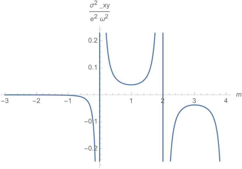
Figure 4: The second order conductivity $\sigma_{xy}^{(2)}$ v.s. the parameter $m$. It is not quantized and non-universal

Based on the Hamiltonian of the simple Chern insulator, the Berry curvature can be analytically computed and be written as

$$\mathcal{F}_{\mu\nu}=\frac{1}{2}\epsilon_{\alpha\beta\gamma}\hat{d}_{\alpha}\partial_{k_{\mu}}\hat{d}_{\beta}\partial_{k_{\nu}}\hat{d}_{\gamma}$$ (126)

with

$$\hat{d}_{\alpha}(\boldsymbol{k})=d_{\alpha}(\boldsymbol{k})/d(\boldsymbol{k}).$$ (127)

Hence, we have the expression for $\mathcal{F}_{xy}$,

$$\mathcal{F}_{xy}=\frac{-\cos(k_{y})-\cos(k_{x})(1+(-2+m)\cos(k_{y}))}{2((-2+m+\cos(k_{x})+\cos(k_{y}))^{2}+\sin(k_{x})^{2}+\sin(k_{y})^{2})^{3/2}}.$$ (128)

The numerical results of the second-order conductivity are shown in Fig.4. The second-order conductivity is not zero or quantized. It is non-universal.

References

- Wan et al. (2011) X. Wan, A. M. Turner, A. Vishwanath, and S. Y. Savrasov, Physical Review B - Condensed Matter and Materials Physics 83 (2011), 10.1103/PhysRevB.83.205101.
- Novoselov et al. (2004) K. S. Novoselov, a K Geim, S. V. Morozov, D. Jiang, Y. Zhang, S. V. Dubonos, I. V. Grigorieva, and a a Firsov, Science (New York, N.Y.) 306 (2004).
- Armitage et al. (2018) N. P. Armitage, E. J. Mele, and A. Vishwanath, Reviews of Modern Physics 90 (2018), 10.1103/RevModPhys.90.015001.
- Peskin and Schroeder (2015) M. Peskin and D. Schroeder, An Introduction To Quantum Field Theory (Frontiers in Physics) (CRC Press, 2015).
- Adler (1969) S. L. Adler, Physical Review 177, 2426 (1969).
- Bell and Jackiw (1963) J. Bell and R. Jackiw, Crossref, ISI, ADS (1963).
- Else et al. (2021) D. V. Else, R. Thorngren, and T. Senthil, Phys. Rev. X 11, 021005 (2021).
- Nielsen and Ninomiya (1983) H. B. Nielsen and M. Ninomiya, Physics Letters B 130 (1983), 10.1016/0370-2693(83)91529-0.
- Burkov (2015) A. Burkov, Journal of Physics: Condensed Matter 27, 113201 (2015).
- Adler and Bardeen (1969) S. L. Adler and W. A. Bardeen, Physical Review 182 (1969), 10.1103/PhysRev.182.1517.
- Wen (2004) X.-G. Wen, Quantum field theory of many-body systems: from the origin of sound to an origin of light and electrons (OUP Oxford, 2004).
- Zhang and Hu (2001) S.-C. Zhang and J. Hu, Science 294, 823 (2001).
- Son and Spivak (2013) D. T. Son and B. Z. Spivak, Physical Review B - Condensed Matter and Materials Physics 88 (2013), 10.1103/PhysRevB.88.104412.
- Lee et al. (2018) J. Lee, J. Pixley, and J. D. Sau, Physical Review B 98, 245109 (2018).
- Hagen (1967) C. R. Hagen, Il Nuovo Cimento B Series 10 51 (1967), 10.1007/bf02712329.
- Georgi and Rawls (1971) H. Georgi and J. M. Rawls, Physical Review D 3 (1971), 10.1103/PhysRevD.3.874.
- Shei (1972) S. S. Shei, Physical Review D 6 (1972), 10.1103/PhysRevD.6.3469.
- Avdoshkin et al. (2020) A. Avdoshkin, V. Kozii, and J. E. Moore, Physical Review Letters 124 (2020), 10.1103/PhysRevLett.124.196603.
- Rylands et al. (2021) C. Rylands, A. Parhizkar, A. A. Burkov, and V. Galitski, Physical Review Letters 126 (2021), 10.1103/PhysRevLett.126.185303.
- Goswami and Tewari (2013) P. Goswami and S. Tewari, Physical Review B 88, 245107 (2013).
- Stephanov and Yin (2012) M. A. Stephanov and Y. Yin, Physical Review Letters 109 (2012), 10.1103/PhysRevLett.109.162001.
- Haldane (2004) F. D. Haldane, Physical Review Letters 93 (2004), 10.1103/PhysRevLett.93.206602.
- Von Delft and Schoeller (1998) J. Von Delft and H. Schoeller, Annalen der Physik 510, 225 (1998).
- Oshikawa (2000) M. Oshikawa, Physical Review Letters 84 (2000), 10.1103/PhysRevLett.84.1535.
- Cho et al. (2017) G. Y. Cho, C. T. Hsieh, and S. Ryu, Physical Review B 96 (2017), 10.1103/PhysRevB.96.195105.
- Wang et al. (2021) C. Wang, A. Hickey, X. Ying, and A. Burkov, Physical Review B 104, 235113 (2021).
- Burkov (2018) A. A. Burkov, Annual Review of Condensed Matter Physics 9 (2018), 10.1146/annurev-conmatphys-033117-054129.
- Ahn and Yang (2017) J. Ahn and B. J. Yang, Physical Review Letters 118 (2017), 10.1103/PhysRevLett.118.156401.
- Giamarchi (2007) T. Giamarchi, Quantum Physics in One Dimension (Oxford university Press, 2007).
- Fujikawa (1980) K. Fujikawa, Physical Review D 21 (1980), 10.1103/PhysRevD.21.2848.
- Diaz et al. (1989) A. Diaz, W. Troost, P. V. Nieuwenhuizen, and A. V. Proeyen, International Journal of Modern Physics A 04 (1989), 10.1142/s0217751x8900162x.
- Stone (1994) M. Stone, Bosonization (World Scientific, 1994).
- Coleman (1975) S. Coleman, Physical Review D 11 (1975), 10.1103/PhysRevD.11.2088.
- Mandelstam (1975) S. Mandelstam, Physical Review D 11, 3026 (1975).
- Luttinger (1960) J. M. Luttinger, Physical Review 119 (1960), 10.1103/PhysRev.119.1153.
- Blagoev and Bedell (1997) K. B. Blagoev and K. S. Bedell, Physical Review Letters 79 (1997), 10.1103/PhysRevLett.79.1106.
- Son and Yamamoto (2012) D. T. Son and N. Yamamoto, Physical review letters 109, 181602 (2012).
- Duval et al. (2006) C. Duval, Z. Horváth, P. A. Horváthy, L. Martina, and P. C. Stichel, Modern Physics Letters B 20 (2006), 10.1142/S0217984906010573.
- Xiao et al. (2005) D. Xiao, J. Shi, and Q. Niu, Physical Review Letters 95 (2005), 10.1103/PhysRevLett.95.137204.
- Karplus and Luttinger (1954) R. Karplus and J. Luttinger, Physical Review 95, 1154 (1954).
- Ashcroft and Mermin (2022) N. W. Ashcroft and N. D. Mermin, Solid state physics (Cengage Learning, 2022).
- Chen et al. (2013) Y. Chen, S. Wu, and A. Burkov, Physical Review B 88, 125105 (2013).
- Alavirad and Sau (2016) Y. Alavirad and J. D. Sau, Physical Review B 94, 115160 (2016).
- Ma and Pesin (2015) J. Ma and D. Pesin, Physical Review B 92, 235205 (2015).
- Zhong et al. (2016) S. Zhong, J. E. Moore, and I. Souza, Physical review letters 116, 077201 (2016).
- Vazifeh and Franz (2013) M. Vazifeh and M. Franz, Physical review letters 111, 027201 (2013).
- Wang and Zhang (2012) Z. Wang and S. C. Zhang, Physical Review X 2 (2012), 10.1103/PhysRevX.2.031008.