Deeper quantum circuits via pseudo-twirling coherent errors mitigation in non-Clifford gates
Abstract
The conventional circuit paradigm, utilizing a limited number of gates to construct arbitrary quantum circuits, is hindered by significant noise overhead. For instance, the standard gate paradigm employs two CNOT gates for the partial ZZ rotation in the quantum Fourier transform, even when the rotation angle is very small. In contrast, certain devices, such as IBM cross-resonance-based devices, can directly implement such operations using their native interaction, resulting in considerably shorter and less noisy implementations for small rotation angles. Unfortunately, beyond noise (incoherent errors), coherent errors stemming from qubit crosstalk and calibration imperfections render these implementations impractical. In Clifford gates such as the CNOT, these errors can be addressed through Pauli twirling (also known as randomized compiling). However, this technique is not applicable to the short non-Clifford native implementations described above. The present work introduces, analyzes, and experimentally demonstrates a technique called Pseudo Twirling to address coherent errors in general gates and circuits. Additionally, we experimentally showcase that integrating pseudo twirling with a quantum error mitigation method called adaptive KIK enables the simultaneous mitigation of both noise and coherent errors in non-Clifford gates. This advancement paves the way for error mitigation in larger circuits than ever before.
In recent years, quantum error mitigation protocols [1, 2, 3, 4, 5, 6, 7, 8, 9] have significantly boosted the performance of quantum computers [10, 11, 5, 12, 13, 14, 15, 16, 17, 18]. These methods are primarily designed for managing incoherent errors (noise) arising from interactions with the environment. However, in addition to incoherent errors, there are also coherent errors that cannot be addressed using the same methods in a scalable manner. Coherent errors pose a significant concern in the development of quantum computers in the foreseeable future. They are often attributed to calibration errors, drift in calibration parameters, or coherent crosstalk interactions between qubits. While hardware continues to advance, the demand for minimizing coherent errors becomes increasingly crucial as circuits grow in size and complexity.
Currently, the most effective approach to address these errors is a method known as Randomized Compiling (RC) [19, 14, 20, 21], also referred to as Pauli twirling. However, this technique is limited to Clifford gates. For Clifford gates such as the CNOT, iswap, and others, RC involves executing an ensemble of circuits that are equivalent in the absence of coherent errors, but each circuit alters the coherent error in a distinct way. After running these circuits and performing post-processing averaging, the coherent error is mitigated, but the resulting transformation is no longer a unitary. In other words, the coherent error is converted into an incoherent error. This conversion is beneficial as incoherent errors can be addressed with QEM (quantum error mitigation) protocols. As demonstrated experimentally in [22] the integration of RC with a QEM method called ‘adaptive KIK’, was imperative for removing coherent errors and obtain accurate results.
Another interesting feature of the RC method is that it converts a general incoherent error channel into a Pauli channel that has a much simpler structure [19]. Due to the reduced degrees of freedom in the Pauli channel compared to general noise, it becomes feasible to employ additional sparsity techniques and efficiently characterize the noise channel of multi-qubit Clifford gates [17, 23, 20]. This key feature is what facilitates two important QEM techniques, PEC [4] and PEA [10]. PEA presently hold the record of the largest circuit that QEM has been applied to – 127 qubit Ising lattice time evolution experiment [10]. The largest depth probed in this experiment was 60 cnots.
Regrettably, RC is restricted to Clifford gates, rendering PEC and PEA inapplicable to non-Clifford multi-qubit gates. Furthermore, circuits consisting solely of Clifford gates can be efficiently simulated, making it pointless to build a powerful quantum computer just for their execution. Although multi-qubit non-Clifford gates are not part of the conventional universal gate set paradigm, they can prove crucial in specific applications, particularly in the era of noisy quantum computers where circuit depth is limited.
As a first example we bring the -qubit quantum Fourier transform [24] that comprises of single-qubit gates and two-qubit gates that execute ZZ rotations with an angle of (and multiples of it). As increases, the gate performs a transformation that is very close to the identity transformation. Such gates can be implemented very rapidly when the correct control signals are available, making them less susceptible to noise. In fact, they can be easily implemented using the native two-qubit cross-resonance interaction [25, 26] exploited in IBM gates, as depicted in Fig. 1a. In contrast, in the gate paradigm, the length of the ZZ rotation gate is determined by the length of two CNOT gates, even when the rotation angle is minute (see 1b).
The second example pertains to the simulation of physical systems. For instance, the transverse Ising lattice model [27] also necessitates fractional ZZ gates. Although the implementation of a native fractional ZZ non Clifford gate is not an obstacle (e.g., in the IBM platform), its incompatibility with RC poses a significant problem. The coherent errors in this gate currently cannot be effectively addressed with existing methods.

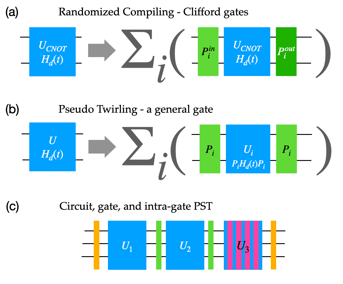
In this work we present a new twirling scheme called ‘pseudo twirling’ (PST). This approach offers three noteworthy characteristics: 1) PST is universally applicable to all gates, including non-Clifford gates. 2) In contrast to RC (Pauli twirling), PST distinguishes between two types of coherent errors: over(under)-rotation errors and uncontrolled coherent errors. Over-rotations typically arise from imperfect initial calibration or a calibration drift. The uncontrolled errors stem from various mechanism ranging from crosstalk between qubits to unwanted interaction generated by the driving field. PST selectively transforms uncontrolled errors into noise, leaving calibration errors unaffected. 3) PST does not produce a Pauli error channel; instead, it appears to generate a distinct, beneficial noise channel. In this paper we present and study these three features. By integrating PST with QEM this research can have an immediate impact on the capabilities of quantum computers.
With the restriction of applying twirling exclusively to Clifford gates removed, PST can be employed within individual components of a gate (intra-gate PST). As we show later, this facilitates more robust mitigation of coherent errors since coherent errors are addressed before they have a chance to accumulate. Additionally, PST’s flexibility allows for its application across an entire circuit, where the twirling occurs at the edges. Although less effective than intra-gate PST, it can capture coherent errors occurring on a scale exceeding that of multi-qubit gates.
We would like to highlight that, after the completion of the theory presented in this paper, we became aware that IBM is also exploring a similar concept. However, we lack specific details regarding their idea and how it was exploited. Our work was conducted entirely independently, and we did not receive any technical or scientific input from IBM or any other entity.
Notations and quantum dynamics in Liouville space
For convenience we shall use Liouville space representation where the density matrix is flattened in column vector and the evolution is described by superoperators operating on this vector from the left . See Appendix I for more details.
Pauli matrices in Liouville space - Let us denote by the product of single-qubit Pauli matrices such that . In Hilbert space the Pauli evolution operator and Pauli Hamiltonian are the same. In Liouville space the two expression differ. A Pauli Hamiltonian in Liouville space is given by while a Pauli evolution operator has the form in Liouville space (see Appendix I). The two are related via the relation . While some of the derivations in this work can be carried our in Hilbert space for clarity and consistency we carry out all calculations in Liouville space. A single exception will be discussed when introduced.
I Description of the PST Methodology
I.1 Regular Randomized Compiling
For clarity, we start by describing the regular randomized compiling/Pauli twirling scheme which is applicable only for Clifford gates. Let stand for the evolution operator of an ideal Clifford gate and let stand for the evolution operator of the noisy realization of . may encompass both noise and coherent errors, but, for the moment, we will concentrate on the noise-free scenario where only coherent errors take place.
As shown in Fig. 2a, in RC, is replaced by an averaged operator, with each element "twirled" by an n-qubit Pauli operators and .
is chosen in such a way that it yields in the absence of coherent or incoherent errors. This condition of invariance can be expressed as , leading to the determination of as . Therefore, is defined based on the selected . Up to his point it appears as we have not used the fact that is Clifford. However, since Pauli operators are stabilizers of the Clifford gates, it is guaranteed that if is a Pauli operator, then is also a Pauli operator. Conversely, if the ideal gate is non-Clifford, may involve multi-qubit interactions, introducing noise and coherent errors comparable to those RC aims to correct. These additional errors could potentially worsen the twirled operator. Thus, a significant advantage of Pauli Twirling lies in the experimental simplicity of the twirling operations, which involve very low levels of coherent and incoherent errors.
Notably, the full number of twirlings for -qubit gate, , can swiftly grow to a very substantial value. This becomes particularly evident when considering sequences of twirled gates. Fortunately, there is no need to sum over all possible Pauli operators. It suffices to sample a subset from the set to obtain the average value. Nevertheless, for the sake of simplicity we will maintain the use of .
To gain a better grasp of how RC operates, let us express as , where represents the error channel that encompasses all errors. This decomposition always exists when the dynamics of the gate constitute a completely positive map. Substituting it into the twirling formula, we obtain:
Hence, twirling a Clifford gate with Pauli operators is equivalent to twirling its noise channel. Note however that for the noise twirling . Furthermore, we can utilize the fact that Pauli operators form a complete basis, allowing any matrix to be represented as where is the transpose operation. It can be shown that, after Pauli twirling, transforms into
In this transformation, only the diagonal elements in the diagonal basis remain. This resulting channel is referred to as a Pauli error channel, and it corresponds to randomly applying a Pauli unitary with a probability of . Thus, regardless of the original structure of , Pauli twirling turns it into a Pauli channel.
I.2 Introducing the Pseudo Twirling Protocol
To introduce the concept of pseudo twirling we start with the following observation. Consider a simple non-Pauli gate, such as the two-qubit gate , where for simplicity, we use the notation , . When , this gate is not a Clifford gate. As a starting point, our goal is to create an operation similar to twirling that keeps the functionality of the ideal gate, as in the case of Pauli twirling. If we apply , we get: since and commute. However, , for example, anti-commutes with , and therefore . Our PST protocol is based on the fact that if the Pauli operators anti-commute with the Hamiltonian of , we can simply change the sign of the angle (i.e., the sign of the driving fields) to achieve the desired transformation in the end:
More generally when the driving Hamiltonian is not a single Pauli we can write so that and then the PST twirling takes the form
| (1) |
where equals if and commute, and if they anti-commute. Note that in the definition of we used Pauli matrices in Hilbert space. Mathematically, expression (1) is straightforward, but it should be considered with execution protocol in mind. The right is executed at the beginning of the gate. Then a modified unitary is executed next by changing the sign of some of the control signal. Finally, another is executed at the end of the gate. Importantly, the Hamiltonian of the modified unitary has the same elements as the original Hamiltonian, with only the sign of some terms changing. From an experimental perspective, this implies that implementing PST is no more challenging than implementing the original unitary.
The main operational differences between RC and pseudo twirling are as follows:
-
•
In RC, the Pauli gates at the beginning and end are different. In pseudo twirling, they are always the same.
-
•
In RC, the operation between the Pauli gates (the gate itself) is always the same. Conversely, in PST, the operation between the Pauli gates depends on the selected Pauli.
-
•
In both methods, the twirling gates are Pauli gates, but in PST, the Pauli gates are also employed to determine the signs of the control signals that drive the gate.
RC and PST are illustrated in Fig. 2a and Fig. 2b respectively. We note that the term ‘pseudo twirling’ reflects not merely an operational difference from standard twirling but also its distinct impact on errors, as discussed in the following two sections. Its effects differs from Pauli twirling in two significant ways: i) it cannot eliminate one type of coherent error, specifically over/under rotations, and ii) it does not transform incoherent errors into a Pauli channel. Nevertheless, we will show and demonstrate that these differences do not diminish the usefulness of pseudo twirling.
I.3 PST Impact on Coherent Errors
While the impact of PST on strong coherent and incoherent errors is should be further studied we do understand its effect on weak error. Through the Magnus expansion [28] and the interaction picture, we find that the PST of a circuit with a coherent error induced by a Hamiltonian term can be expressed as follows:
where is the ideal evolution operator of the non-twirled gate. is in Liouville space which is related to the Hilbert space Hamiltonian through the relation
| (2) |
The first order approximation in is
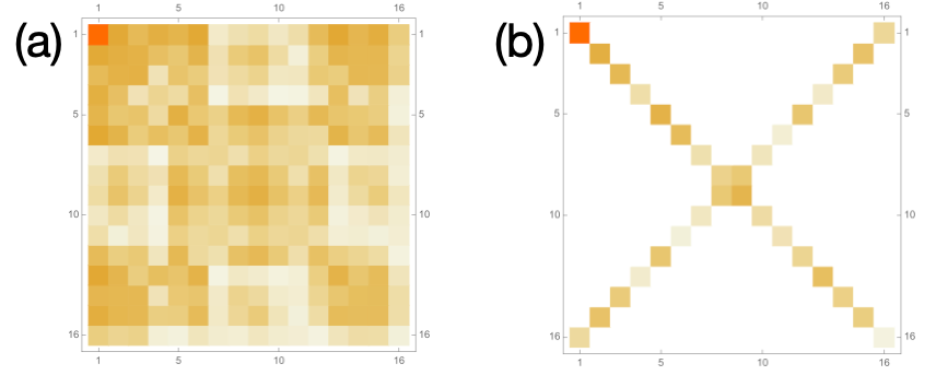
where the last step follows from the fact that is a Pauli twirling of . As such the twirling eliminates the leading term in the coherent error since . This explains why PST suppresses coherent errors. Higher order terms do not have the structure of (2) and require a more elaborate analysis. Figure 3(a) shows the error map in the Pauli basis of the gate with an added coherent error. In Figure 3(b) the noise map of the same gate after applying PST is plotted.
I.4 PST and Noise
In the context of Pauli twirling, it is evident that the resulting incoherent error exhibits a Pauli error channel structure. However, in the case of PST, this may not hold true, even in the first order. If we revisit the analysis from the previous section but consider a general Lindblad dissipator describing a Markovian trace-preserving noise, we obtain:
where . The Pauli twirling of turns it into a Pauli, however, the summation over additional rotation by make the whole expression a non Pauli channel. Yet, since is Pauli channel, it is Hermitian and consequently, is also Hermitian. We conclude that PST makes the leading order of the noise Hermitian. Please refer to our numerical results section for supporting simulations. We observe that the anti-Hermitian part of the noise, can decrease by a factor of several hundreds or more after applying PST. The impact of PST on higher-order noise terms is left for future work.
Interestingly, in [29] it was shown that to a leading order, Hermitian noise does not degrade the result of control-free phase estimation. To exploit this feature, the authors applied randomized compiling for transforming the noise into a Pauli channel (which is Hermitian). However this technique can only be applied to Clifford gates. PST can pose an alternative for making the leading order of the noise Hermitian even for short low-noise non-Clifford gates.
II PST features - Limitations and Opportunities
II.1 PST and Calibration
There are two types of coherent errors: controllable errors arising from miscalibration of controllable degrees of freedom which we refer to a over/under rotation error, and uncontrollable errors such as crosstalk that do not depend on the control signals (driving fields). While RC makes no distinction and effectively mitigate both types of coherent errors, PST specifically addresses crosstalk and other uncontrollable coherent errors. Crucially over/under rotation errors that are crucial in gate calibration are not affected by PST. This feature opens new possibilities.
Initially, it may seem that this limitation renders PST only a partial solution, as it cannot transform calibration errors into incoherent errors. However this exact limitation can become an advantage in gate calibration. A proper calibration is always a good practice. Even when RC is applicable, miscalibrated gates introduce access noise that makes the QEM task more challenging. PST, on the other hand, does not convert rotation errors into incoherent errors. This characteristic allows for the application of PST during the calibration process, simplifying it by reducing certain coherent errors, such as crosstalk errors, while leaving those associated with the calibration itself untouched. Consequently, integrating PST into the calibration process can facilitate the high-accuracy calibration necessary for circuits with significant depth.
For example consider the case of cross-resonance gate where the leading driving Hamiltonian term is , where is the amplitude of the drive and is the phase of the drive. After applying PST we have:
Note that in this case it is not possible to directly control the amplitudes of and separately. In principle, such control can be achieve by changing the sign of the phase as well. However, by doing the explicit summation find that and therefore the PST summation nulls the term even without modifying the sign of the phase. This leads to a simplification in the calibration procedure: rather than fine-tune to zero and then fine tune , it is possible to coarsely set and the calibrate until achieves the desired value.
II.2 PST application alternatives
Since PST is versatile and can be applied to any gate or circuit, there are various alternatives for its application within a given circuit. Some options include:
-
•
Circuit PST - Applying PST to the entire circuit, with the twirling gates positioned solely at the circuit’s edges.
-
•
Gate PST- Applying PST on a per-gate basis.
-
•
Intra-gate PST - Implementing PST within each gate.
-
•
Hybrid PST-RC - In Clifford gates, combine Intra-gate PST with RC, or RC with circuit PST
The first three options are illustrate in Fig. 2c.
Given the absence of a clear cost analysis, it appears advantageous
to consider all three levels of implementation, or at the very least,
the first and third options. Implementing PST in shorter intervals
(intra-gate PST) is an effective strategy to prevent the accumulation
and growth of coherent error. Employing PST across the entire circuit
is also beneficial, as it can mitigate the accumulation of errors
resulting from non-local (non-gate-based) mechanisms.
Intra-Gate PST
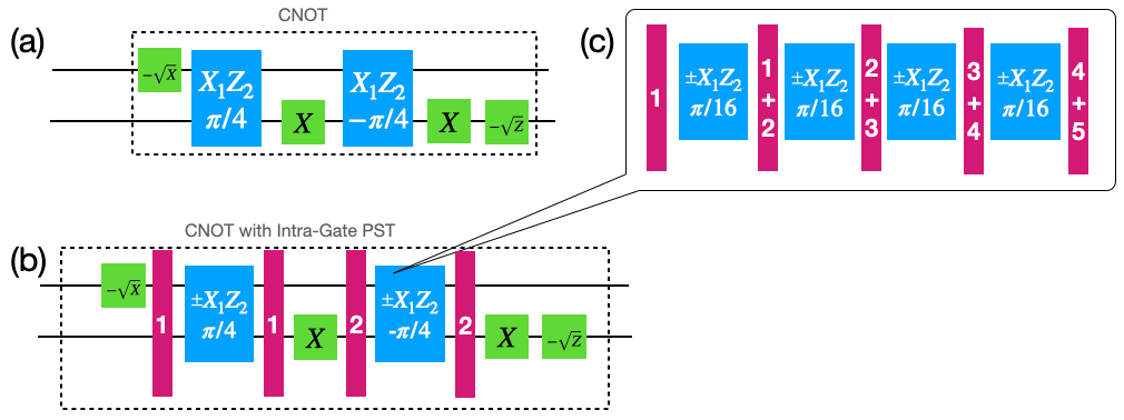
Let us elaborate on the intra-gate PST approach. Taking the example of the cross-resonance CNOT gate [25] depicted in Fig. 4a, each non-Clifford element (pulse) can be pseudo-twirled independently within the PST framework as shown in Fig. 4b. This contrasts with RC, which cannot be applied to the non-Clifford elements of the gate. Additionally, each one of two segments of the cross-resonance pulse can be divided into multiple shorter pulses, allowing for the application of PST across these smaller segments (Fig. 4c). The prospective advantage here is to mitigate coherent errors before they accumulate. More detailed results are available in the Preliminary Results section.
In the context of Clifford gates such as the CNOT, conventional RC can be applied at the gate level, while employing PST within the gate’s internal elements. RC aids in addressing calibration errors that PST does not address. Meanwhile, PST’s role is to decrease the level of coherent errors experienced by RC, resulting in reduced incoherent errors and less fluctuations in the post-processing averaging.
II.3 Integration and Compatibility with QEM
It is evident that PST, by itself, will only provide a limited solution to errors in quantum devices, as it converts coherent errors into incoherent errors, which still need to be addressed using QEM. Therefore, the impact of PST largely depends on its compatibility with QEM methods. While some error mitigation protocols are expected to be compatible with PST, others that rely on the twirled noise to be a Pauli channel, such as PEC and PEA, may not be. In what follows we demonstrate numerically and experimentally that PST is not only compatible with the Adaptive KIK QEM method [22] it actually improve the resilience of the method to crosstalk.
III Numerical Results
III.1 Intra-Gate PST
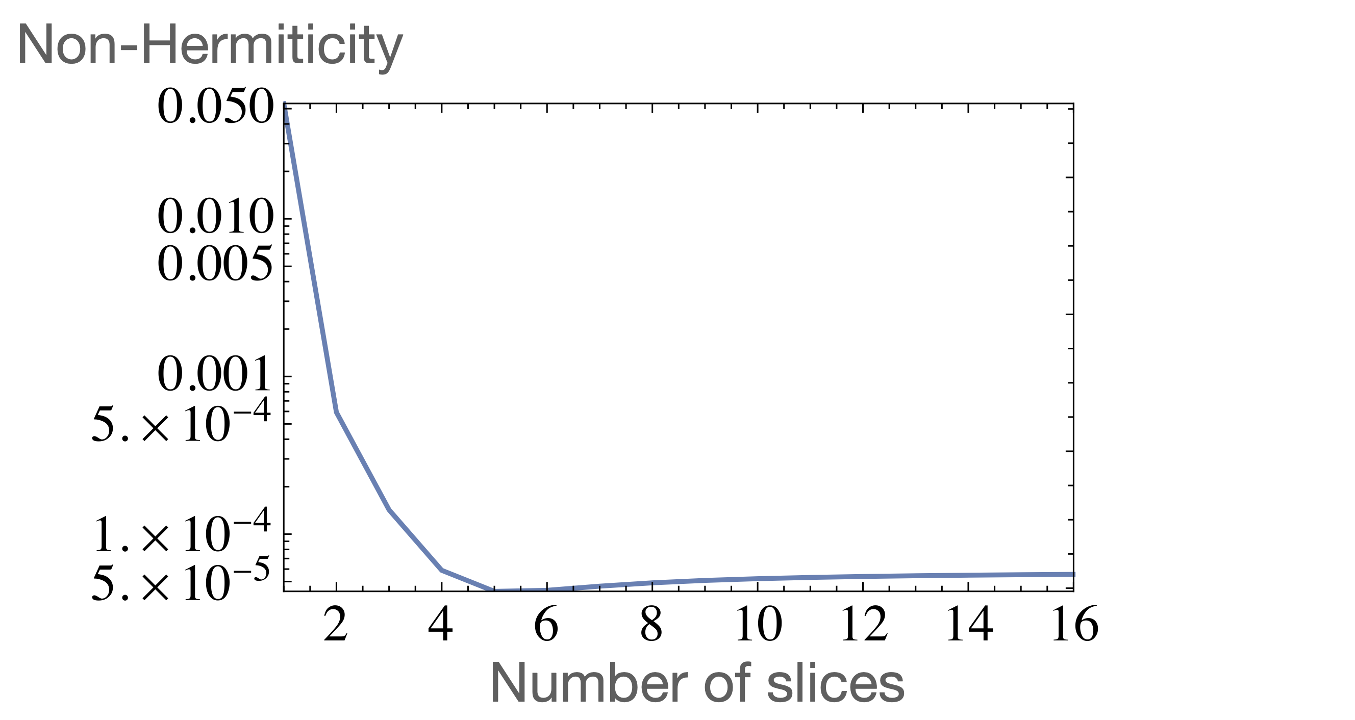
As alluded to in Fig. 4c, implementing PST on smaller segments of a pulse allows for further improvement in coherent error suppression. To illustrate this point, we conducted a simulation involving the slicing of a cross-resonance pulse. We applied PST to each slice and plotted the error in the entire evolution compared to the ideal cross-resonance pulse. The results, shown in Fig. 5, reveal that error suppression enhances as the number of slices increases. We observed that the level of suppression is inversely proportional to the number of slices (indicated by the orange curve). Intuitively, since PST suppress the leading order of the coherent error it becomes more effective when applied to thiner slices where the higher order terms (of the coherent error) are negligible. Thus, in thin slices the PST mitigates the coherent error before it has chance to accumulate.
Clearly, there comes a point where the length of the slice becomes comparable to that of the PST Pauli operators, and further slicing will not be possible. Additionally, residual coherent errors in the PST Pauli operators may also set a performance limit. Nonetheless, our results suggest that before reaching these limiting factor intra-gate PST improves the coherent error suppression.
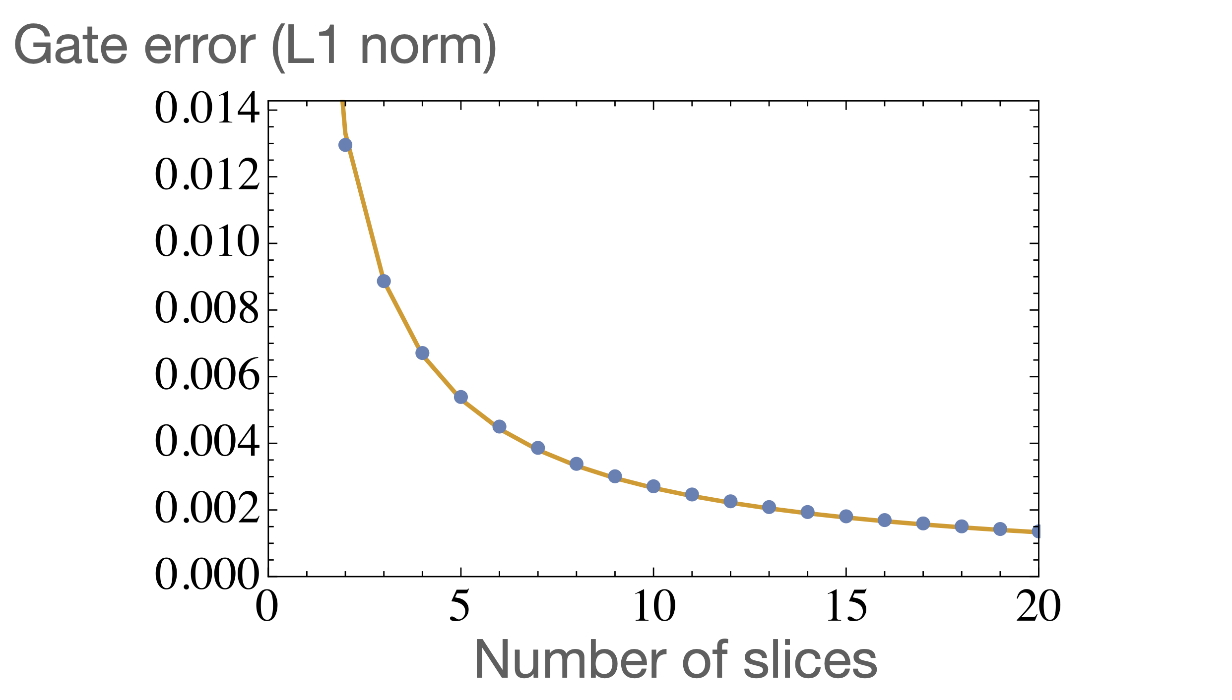 Figure 5: Numerical simulation illustrating the impact
of intra-gate PST on coherent errors. In this example, the ideal evolution
corresponds to the cross-resonance pulse utilized in IBM’s implementation
of the CNOT gate. Slicing the pulses into multiple shorter segments
and applying PST to each of them results in a reduction of the final
coherent error. The x-axis represents the number of slices (pulses),
while the y-axis indicates the trace norm distance from the ideal
pulse. The solid orange line corresponds to a fit using the equation
/(number of slices), where is the fitting parameter.
Figure 5: Numerical simulation illustrating the impact
of intra-gate PST on coherent errors. In this example, the ideal evolution
corresponds to the cross-resonance pulse utilized in IBM’s implementation
of the CNOT gate. Slicing the pulses into multiple shorter segments
and applying PST to each of them results in a reduction of the final
coherent error. The x-axis represents the number of slices (pulses),
while the y-axis indicates the trace norm distance from the ideal
pulse. The solid orange line corresponds to a fit using the equation
/(number of slices), where is the fitting parameter.
III.2 PST as a “Hermitianizer” of the Error Channel
To illustrate the effect of PST on incoherent errors, we consider the same cross-resonance pulse slicing example shown in Fig. 5, but this time with coherent errors replaced by incoherent errors. Figure 6 displays the non-hermiticity measure of the error channel as a function of the number of slices. This measure equals one for anti-Hermitian operators and zero for Hermitian operators. The sharp drop of the curve illustrates our analytical finding that PST makes the error channel more Hermitian. We have confirmed this in different circuits and with various error models, including coherent errors.
III.3 Integration of PST and Quantum Error Mitigation
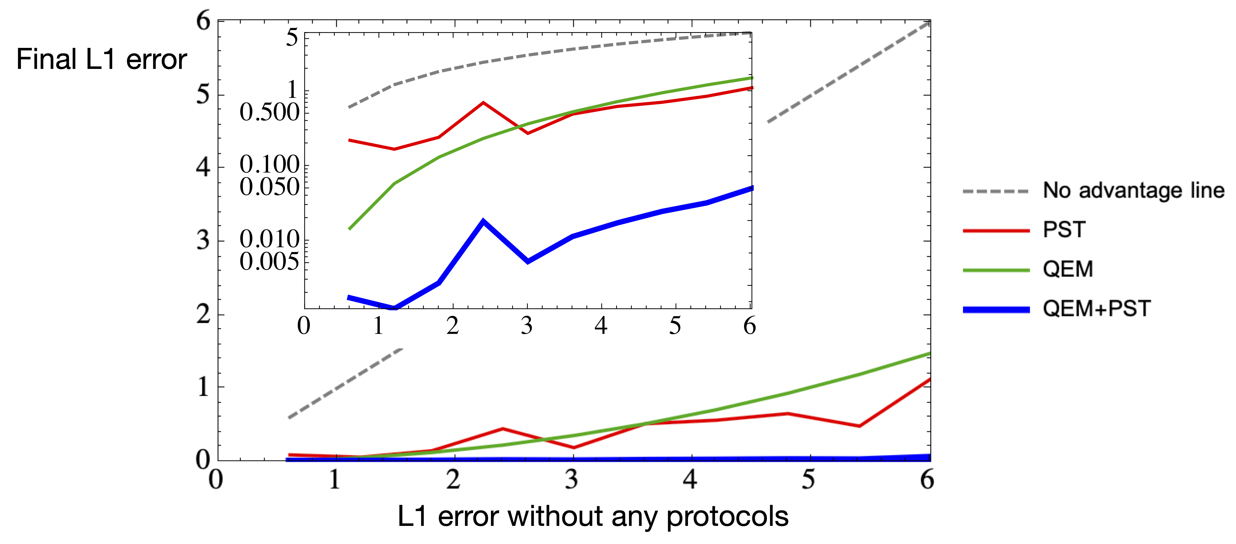
As explained earlier, PST alone will not suffice. Ideally, it should completely eliminate coherent errors and transform the noise into a fully Hermitian noise channel. However, the resulting noise channel can still be too strong to extract meaningful results from a given quantum computer. Therefore, PST must be followed by a quantum error mitigation (QEM) protocol. We chose the ‘Adaptive KIK’ QEM method [22] due to its is operational simplicity and its compatibility with non-Clifford gates. To exemplify the compatibility of PST with this QEM method, we conducted a three-qubit transverse Ising model simulation with both coherent and incoherent errors. Figure 7 illustrates that PST significantly enhances Adaptive-KIK performance, as evident from the shift from the green curve to the blue curve. To emphasize the insufficiency of PST alone, we have also plotted in red the error when PST is applied without KIK.
IV Experimental Results
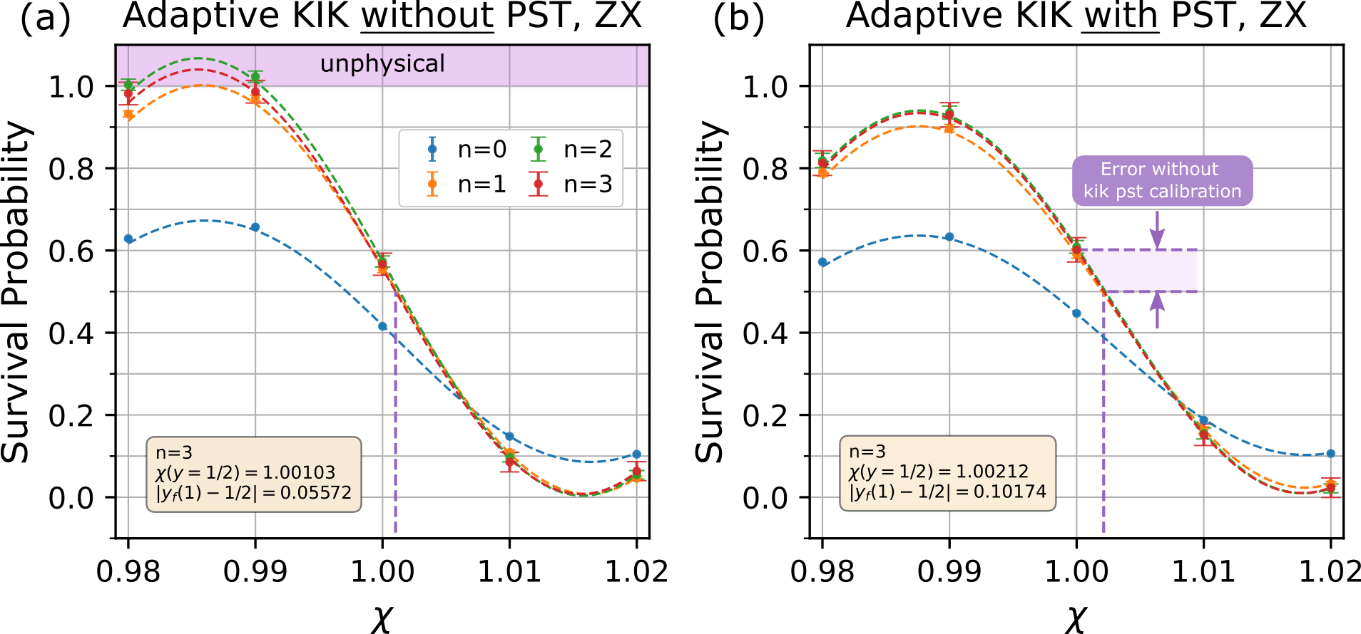
To illustrate the utility of PST to gate-calibration we run a ‘deep calibration’ experiment where we calibrate a sequence of 81 ZX echo cross resonance pulses. Such a large number of repetitions amplifies the smallest coherent errors. Yet, a trivial execution of such a long circuit is prone to substantial incoherent errors (noise) that will dramatically effect the calibration curve and lead to an erroneous calibration as demonstrated in [22]. Thus, we use the Adaptive KIK [22] QEM methodology for removing the incoherent errors. We measure the probability to measure the system in the initial (survival probability) after 81 sequences for different stretch factor of the CR pulse amplitude. A value of one corresponds to the default amplitude value provided by IBM.
By comparing the results of applying KIK with and without PST we observe in Fig. 8 that i) with PST (Fig. 8b) the KIK converges faster (less mitigation orders are needed) compared to the same experiment without PST (Fig. 8a). ii) The value of the calibrated amplitude is affected by the PST. iii) Without PST for some amplitudes we get unphysical values. to the best of our knowledge, such non-physical values can occur for two reasons: 1) the mitigation order is too small with respect to the window size parameter in the KIK method (see simulations in the appendix of [22]) and the other reason is non-Markovian effects. One of the sources of non-Markovian effect in the present setup is crosstalk interaction with adjacent qubits. If the order is too low we expect the unphysical values to disappear as the order increases. Indeed appear to be more physical than , yet, since the two result differ convergence is not observed and we cannot confirm that unphysical values disappear in higher orders. Moreover, when the mitigation order is too low PST is not expected to help. The fact that PST does removes the unphysical values and speed up convergence suggest that that the unphysical value without PST are related to non-Markovian effects. We point out that in other experiments we observed this behavior when neighboring idle qubits are not protected using dynamical decoupling.
Note that what we control is the actual drive of the ZX term . In PST calibration it is not needed to know explicitly, is scanned until the survival probability obtain the value of which means that (the value that corresponds to CR pulse).
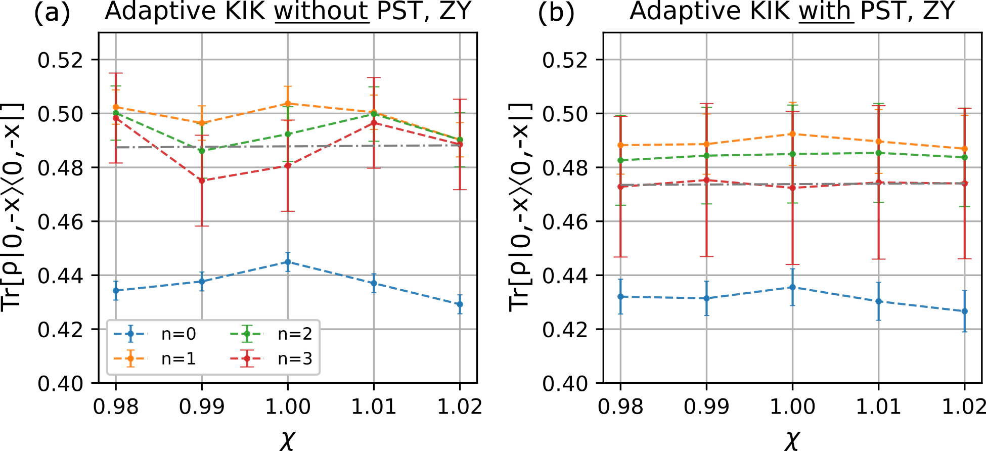
One might worry that for a residual ZY term will remain and generate a coherent error. However as explained in is Sec., and demonstrated experimentally next, PST eliminated the small terms. To experimentally demonstrate this point we carry out a variant of the previous experiment where a single-qubit rotation is added to the controlled qubit (in interaction the right qubit is the controlled qubit) just before the measurement. This makes the survival probability sensitive to rather than to . Without PST it is expected that the outcomes will show some dependence on the amplitude since is not exactly zero if is not perfectly calibrated to zero. As show in Fig. 9b after applying PST and KIK we find that calibration curve is flat as expected. As a comparison we show the result without PST on 9a. The mean square error in fitting a straight line to the data is presented in the yellow boxes.
Finally we point out an important observation regarding the use of virtual Z gates in the pseudo twirling gates. Due to their simplicity and very low error rates, virtual Z gates are very popular in quantum computers setups. In short, the Z rotation can pushed further dow the circuit by modifying the phases of pulses that generate gates that do not commute with Z. However, despite their advantage, as explained in Appendix II , virtual gate are not suitable for PST. Thus, in our experiment we implement the gate by changing the phase of the pulse and not by implementing (where where is a virtual Z gate. For gate we use or . When the noise is very weak these two options are equivalent. We show that using virtual gates make twirling that are suppose to be different become the same.
V Summary and concluding remarks
The working hypothesis underlying the present paper is that shorter gates facilitate deeper circuits. However, the coherent errors in short multi-qubit gates cannot be addressed with randomized compiling (Pauli twirling) techniques as it hinges on the assumption that the ideal gates are Clifford gates. Our analytical, numerical, and experimental findings indicate that pseudo twirling can bridge this gap and successfully mitigate coherent errors in non-Clifford gates. Pseudo twirling possesses three advantages that separate it from the established randomized compiling approach: i) Applicability to Non-Clifford Gates: It enables the implementation of significantly shorter gates, resulting in lower noise accumulation compared to Clifford-based implementations. ii) Intra-Gate Coherent Error Suppression: Pseudo twirling allows for the suppression of coherent errors within gates and sliced pulses, leading to substantial improvement in coherent error suppression. iii) Circuit-PST: By applying pseudo twirling also at the edges of a circuit, it is possible to suppress non-local multi-qubit coherent errors.
Moreover, the successful integration of PST with the Adaptive-KIK error mitigation method leads to a substantial performance boost. This boost can be instrumental in achieving quantum advantage in a wide range of fields, including particle physics, condensed matter, quantum chemistry, and more.
Acknowledgements.
The authors acknowledge the use of IBM Quantum services for this work. The views expressed are those of the authors, and do not reflect the official policy or position of IBM or the IBM Quantum team. We thank IAI/ELTA Systems for the assistance in running the experiments. Raam Uzdin is grateful for support from the Israel Science Foundation (Grant No. 2556/20).References
- Cai et al. [2022] Z. Cai, R. Babbush, S. C. Benjamin, S. Endo, W. J. Huggins, Y. Li, J. R. McClean, and T. E. O’Brien, arXiv preprint arXiv:2210.00921 (2022).
- Endo et al. [2018] S. Endo, S. C. Benjamin, and Y. Li, Physical Review X 8, 031027 (2018).
- Suzuki et al. [2022] Y. Suzuki, S. Endo, K. Fujii, and Y. Tokunaga, PRX Quantum 3, 010345 (2022).
- Temme et al. [2017] K. Temme, S. Bravyi, and J. M. Gambetta, Physical review letters 119, 180509 (2017).
- Huggins et al. [2021] W. J. Huggins, S. McArdle, T. E. O’Brien, J. Lee, N. C. Rubin, S. Boixo, K. B. Whaley, R. Babbush, and J. R. McClean, Physical Review X 11, 041036 (2021).
- Koczor [2021] B. Koczor, Physical Review X 11, 031057 (2021).
- He et al. [2020] A. He, B. Nachman, W. A. de Jong, and C. W. Bauer, Phys. Rev. A 102, 012426 (2020).
- Strikis et al. [2021] A. Strikis, D. Qin, Y. Chen, S. C. Benjamin, and Y. Li, PRX Quantum 2, 040330 (2021).
- Li and Benjamin [2017] Y. Li and S. C. Benjamin, Physical Review X 7, 021050 (2017).
- Kim et al. [2023] Y. Kim, A. Eddins, S. Anand, K. X. Wei, E. Van Den Berg, S. Rosenblatt, H. Nayfeh, Y. Wu, M. Zaletel, K. Temme, et al., Nature 618, 500 (2023).
- Kandala et al. [2019] A. Kandala, K. Temme, A. D. Corcoles, A. Mezzacapo, J. M. Chow, and J. M. Gambetta, Nature 567, 491 (2019).
- Song et al. [2019] C. Song, J. Cui, H. Wang, J. Hao, H. Feng, and Y. Li, Science advances 5, eaaw5686 (2019).
- Zhang et al. [2020] S. Zhang, Y. Lu, K. Zhang, W. Chen, Y. Li, J.-N. Zhang, and K. Kim, Nature communications 11, 587 (2020).
- Hashim et al. [2021] A. Hashim, R. K. Naik, A. Morvan, J.-L. Ville, B. Mitchell, J. M. Kreikebaum, M. Davis, E. Smith, C. Iancu, K. P. O’Brien, I. Hincks, J. J. Wallman, J. Emerson, and I. Siddiqi, Phys. Rev. X 11, 041039 (2021).
- Guimarães et al. [2023] J. D. Guimarães, J. Lim, M. I. Vasilevskiy, S. F. Huelga, and M. B. Plenio, PRX Quantum 4, 040329 (2023).
- Sagastizabal et al. [2019] R. Sagastizabal, X. Bonet-Monroig, M. Singh, M. A. Rol, C. Bultink, X. Fu, C. Price, V. Ostroukh, N. Muthusubramanian, A. Bruno, et al., Physical Review A 100, 010302 (2019).
- Van Den Berg et al. [2023] E. Van Den Berg, Z. K. Minev, A. Kandala, and K. Temme, Nature Physics , 1 (2023).
- Shtanko et al. [2023] O. Shtanko, D. S. Wang, H. Zhang, N. Harle, A. Seif, R. Movassagh, and Z. Minev, arXiv preprint arXiv:2307.07552 (2023).
- Wallman and Emerson [2016] J. J. Wallman and J. Emerson, Physical Review A 94, 052325 (2016).
- Harper et al. [2020] R. Harper, S. T. Flammia, and J. J. Wallman, Nature Physics 16, 1184 (2020).
- Knill [2004] E. Knill, arXiv preprint quant-ph/0404104 (2004).
- Henao et al. [2023] I. Henao, J. P. Santos, and R. Uzdin, npj Quantum Information 9, 120 (2023).
- Jaloveckas et al. [2023] J. E. Jaloveckas, M. T. P. Nguyen, L. Palackal, J. M. Lorenz, and H. Ehm, arXiv preprint arXiv:2311.11639 (2023).
- Nielsen and Chuang [2002] M. A. Nielsen and I. Chuang, Quantum computation and quantum information (American Association of Physics Teachers, 2002).
- Malekakhlagh et al. [2020] M. Malekakhlagh, E. Magesan, and D. C. McKay, Physical Review A 102, 042605 (2020).
- Sundaresan et al. [2020] N. Sundaresan, I. Lauer, E. Pritchett, E. Magesan, P. Jurcevic, and J. M. Gambetta, PRX Quantum 1, 020318 (2020).
- Suzuki et al. [2012] S. Suzuki, J.-i. Inoue, and B. K. Chakrabarti, Quantum Ising phases and transitions in transverse Ising models, Vol. 862 (Springer, 2012).
- Blanes et al. [2009] S. Blanes, F. Casas, J.-A. Oteo, and J. Ros, Physics reports 470, 151 (2009).
- Gu et al. [2023] Y. Gu, Y. Ma, N. Forcellini, and D. E. Liu, Physical Review Letters 130, 250601 (2023).
- Gyamfi [2020] J. A. Gyamfi, European Journal of Physics 41, 063002 (2020).
Appendix I - Quantum mechanics in Liouville space
Within the conventional Hilbert space framework of Quantum Mechanics, a quantum system of dimension is described by a density matrix which has the dimensions . In addition, a general completely positive quantum operation can be expressed as
| (3) |
where is the transformed density matrix and are Kraus operators that satisfying the relation (being the identity matrix). In the Hilbert space formalism, observables are described by a hermitian operators . The expectation value of for system in the state reads
| (4) |
The Liouville space representation serves as an alternative mathematical formulation that greatly aids in streamlining the expression of quantum states and their transformations. In this model, the density matrix is transformed into a state vector, indicated as , with a dimensionality of , and a quantum transformation is depicted by a superoperator matrix with dimensions .
utilize the scripted notation for a generic quantum operation, its corresponding expression in Liouville space, Eq. (3), is replaced by
| (5) |
Following the methodology of Ref. [30], is the column vector whose first components correspond to the first row of , the next components correspond to the second row of , and so forth. More explicitly the “vec-ing” procedure a generic matrix reads , where is the entry of . With this convention, in Liouville space a Kraus map (3) takes the form [30]
| (6) |
where is the element-wise complex conjugate of . Since unitary map is a special case of Kraus map , is Liouville space a unitary evolution is given by
| (7) |
Equation (6) is follows from the vectorization rule for a product of three matrices , and [30]
| (8) |
where the superscript T denotes transposition (not hermitian conjugate). Equation (6) follows by setting , , and .
Lastly, expectation value (4) of an observable matrix can be neatly expressed in Liouville space using the ’bra’ of . That is, as a column row vector . As result, using the hermiticity of we obtain that of the expectation value of can be written as a ’bra-ket’ inner product of and
| (9) |
Appendix II - The issue with using virtual gates in PST
The basic idea behind the frame rotation used for virtual Z is as follows. Consider the case where we need to implement an gate followed by a transformation U. We can write it as:
For simplicity, we assume that where is some Pauli. If , , then we are done since we have pushed the to the next layer. The idea in virtual gate is to keep pushing the gates all the way to the end of the circuit. Since the measurement is in the computational basis, the final rotation has no impact.
Now let us consider the more interesting case where and anti-commute:
Using the anti-commutation:
Typically will be either or . For example, if it is we get
which means that the physical implementation of just involves changing the phase of the pulse generating . For example, an before the controlled qubit of ZX cross resonance pulse, will manifest in changing the phase of the CR pulse.
Let us consider the PST case
In pseudo twirling, we use Pauli gates so , and therefore the virtualization will amount to changing the sign of the drive without affecting the coherent error
Thus, a virtual Z twirling is equivalent to the identity twirling and will do nothing in this case. In contrast, when using physical Z gates we get:
which twirls the coherent error. Similarly, in IY twirling we aim to generate
However, if is generated via virtual Z: we obtain
Thus, the IY twirling is indistinguishable from IX twirling. While aiming to sample from the full set of twirlings, the use of virtual Z and also Y using virtual Z, decimates the effective set of accessible twirlings and consequently degrades the ability of PST to mitigate the full scope of coherent errors.