Data Attribution for Diffusion Models: Timestep-induced Bias in Influence Estimation

Abstract

Data attribution methods trace model behavior back to its training dataset, offering an effective approach to better understand “black-box” neural networks. While prior research has established quantifiable links between model output and training data in diverse settings, interpreting diffusion model outputs in relation to training samples remains underexplored. In particular, diffusion models operate over a sequence of timesteps instead of instantaneous input-output relationships in previous contexts, posing a significant challenge to extend existing frameworks to diffusion models directly. Notably, we present Diffusion-TracIn that incorporates this temporal dynamics and observe that samples’ loss gradient norms are highly dependent on timestep. This trend leads to a prominent bias in influence estimation, and is particularly noticeable for samples trained on large-norm-inducing timesteps, causing them to be generally influential. To mitigate this effect, we introduce Diffusion-ReTrac as a re-normalized adaptation that enables the retrieval of training samples more targeted to the test sample of interest, facilitating a localized measurement of influence and considerably more intuitive visualization. We demonstrate the efficacy of our approach through various evaluation metrics and auxiliary tasks, reducing the amount of generally influential samples to $\frac{1}{3}$ of its original quantity.

Keywords: Diffusion Models, Interpretability, Data Attribution, Influence

1 Introduction

Deep neural networks have emerged to be powerful tools for the modeling of complex data distributions and intricate representation learning. However, their astounding performance often comes at the cost of interpretability, leading to an increasing research interest to better explain these “black-box” methods. Instance-based interpretation is one approach to explain why a given machine learning model makes certain predictions by tracing the output back to training samples. While these methods have been widely studied in supervised tasks and demonstrated good performance [Koh and Liang, 2017; Yeh et al., 2018; Pruthi et al., 2020], there is limited exploration of their application in unsupervised settings, especially for generative models [Kingma and Welling, 2013; Goodfellow et al., 2020; Ho et al., 2020]. In particular, diffusion models represent a state-of-the-art advancement in generative models and demonstrate remarkable performance in a variety of applications such as image generation, audio synthesis, and video generation [Kong et al., 2020; Dhariwal and Nichol, 2021; Ho and Salimans, 2022; Saharia et al., 2022; Hertz et al., 2022; Li et al., 2022; Ho et al., 2022]. The prevailing generative agents in creative arts such as Stable Diffusion [Rombach et al., 2022] also call for fair attribution methods to acknowledge the training data contributors. Nonetheless, the interpretability and attribution of diffusion models remain an under-explored area [Georgiev et al., 2023; Dai and Gifford, 2023].

Compared to traditional supervised settings, the direct extension of instance-based interpretation to diffusion models is challenging due to the following factors. First, the diffusion objective involves an expectation over the injected noise $\epsilon\sim\mathcal{N}(0,I)$, hence a precise computation is impractical. Second, diffusion models operate over a sequence of timesteps instead of instantaneous input-output relationships. Although each timestep is weighted equally during the training process, we observe that certain timesteps can exhibit high gradient norm. This means the gradient of the diffusion loss function with respect to model parameters is dominantly large relative to all other timesteps (Figure 1). As most instance-based explanation models utilize this first-order gradient information, such biased gradient norms can propagate its domination into the influence estimation for diffusion models. In practice, specifically, timesteps are often uniformly sampled during training. Therefore a training sample that happens to be trained on certain timesteps may exhibit higher-than-usual gradient norms, and thus be characterized as “generally influential” to various completely different test samples.

We present Diffusion-TracIn and Diffusion-ReTrac to demonstrate and address the existing difficulties. Diffusion-TracIn is a designed extension of TracIn [Pruthi et al., 2020] to diffusion models that incorporates the denoising timestep trajectory. This approach showcases instances where influence estimation is biased. Subsequently, we introduce Diffusion-ReTrac as a re-normalization of Diffusion-TracIn to alleviate the dominating norm effect.

Our contributions are summarized as follows:

1. Propose Diffusion-TracIn as a designed extension to diffusion models that incorporates and effectively approximates the timestep dynamics.

2. Identify and investigate the timestep-induced gradient norm bias in diffusion models, providing preliminary insights into its impact on influence estimation.

3. Introduce Diffusion-ReTrac to mitigate the timestep-induced bias, offering fairer and targeted data attribution.

4. Illustrate and compare the effectiveness of the proposed approach on auxiliary tasks.

2 Related Work

Data attribution methods trace model interpretability back to the training dataset, aiming to answer the following counterfactual question: which training samples are most responsible for shaping model behavior?

2.1 Influence Estimations

Influence functions quantify the importance of a training sample by estimating the effect induced when the sample of interest is removed from training [Koh and Liang, 2017]. This method involves inverting the Hessian of loss, which is computationally intensive and can be fragile in highly non-convex deep neural networks [Basu et al., 2020]. Representer Point is another technique that computes influence using the representer theorem, yet relies on the assumption that attribution can be approximated by the final layer of neural networks, which may not hold in practice [Yeh et al., 2018]. For diffusion models, the application of influence functions is significantly hindered by its computational expense while extending the representer point method is ambiguous due to the lack of a natural “final layer.” Pruthi et al. introduced TracIn to measure influence based on first-order gradient approximation that does not rely on optimality conditions [Pruthi et al., 2020]. Recently, TRAK is introduced as an attribution method for large-scale models, which requires a designed ensemble of models and hence is less suitable for naturally trained models [Park et al., 2023].

In this paper, we extend the TracIn framework to propose an instance-based interpretation method specific to the diffusion model architecture. To address the challenges arose, we present Diffusion-ReTrac that re-normalizes the gradient information and effectively accommodates the timesteps dynamics. Previous works have utilized similar re-normalization techniques to enhance influence estimator performance in supervised settings. Barshan et al. reweight influence function estimations using optimization objectives that place constraints on global influence, enabling the retrieval of explanatory examples more localized to model predictions [Barshan et al., 2020]. Gradient aggregated similarity (GAS) leverages re-normallization to better identify adversarial instances [Hammoudeh and Lowd, 2022]. These works align well with our studies in understanding the localized impact of training instances on model behavior.

2.2 Influence in Unsupervised Settings

The aforementioned methods address the counterfactual question in supervised settings, where model behavior may be characterized in terms of model prediction and accuracy. However, extending this framework to unsupervised settings is non-trivial due to the lack of labels or ground truth. Prior works explore this topic and approach to compute influence for Generative Adversarial Networks (GAN) [Terashita et al., 2021] and Variational Autoencoders (VAE) [Kong and Chaudhuri, 2021]. Previous work in diffusion models quantifies influence through the use of ensembles, which requires training multiple models with subsets of the training dataset, making it unsuitable for naturally trained models [Dai and Gifford, 2023]. Journey TRAK applies TRAK [Park et al., 2023] to diffusion models and attributes each denoising timestep individually [Georgiev et al., 2023], which is less interpretable since the diffusion trajectory spans multiple timesteps and thus a single-shot attribution is more holistic. Additionally, D-TRAK presents counter-intuitive findings suggesting that theoretically unjustified design choices in TRAK result in improved performance, emphasizing the need for further exploration in data attribution for diffusion models [Zheng et al., 2023]. These works are complementary to our studies and contribute to a more comprehensive understanding of instance-based interpretations in unsupervised settings.

2.3 Areas of Application

Data attribution methods prove valuable across a wide range of domains, such as outlier detection, data cleaning, data curating, and memorization analysis  [Khanna et al., 2019; Liu et al., 2021; Kong et al., 2021; Lin et al., 2022; Feldman, 2020; van den Burg and Williams, 2021]. The adoption of diffusion models in artistic pursuits, such as Stable Diffusion and its variants, has also gained substantial influence [Rombach et al., 2022; Zhang et al., 2023]. This then calls for fair attribution methods to acknowledge and credit artists whose works have shaped these models’ training. Such methods also become crucial for further analyses related to legal and privacy concerns [Carlini et al., 2023; Somepalli et al., 2023].

3 Preliminaries

3.1 Diffusion Models

Denoising Diffusion Probabilistic Models (DDPMs) [Ho et al., 2020] are a special type of generative models that parameterized the data as $p_{\theta}(x_{0})=\int p_{\theta}(x_{0:T})\,dx_{1:T}$, where $x_{1},\dots,x_{T}$ are latent variables of the same dimension as the input. The inner term $p_{\theta}(x_{0:T})$ is the reverse process starting at the standard normal $p(x_{T})=\mathcal{N}(x_{T};0,I)$, which is defined by a Markov chain:

$$p_{\theta}(x_{0:T})=p(x_{T})\prod_{t=1}^{T}p_{\theta}(x_{t-1}|x_{t}),$$ (1)

where $p(x_{t-1}|x_{t})=\mathcal{N}(x_{t-1};\mu_{\theta}(x_{t},t),\Sigma_{\theta}(x_{t},t))$. The reverse process is learnable and fixed to a Markov Chain based on a variance scheduler $\beta_{1},\dots,\beta_{T}$. Notably, efficient training can be achieved by stochastically selecting timesteps for each sample. DDPM further simplifies the loss by re-weighting each timestep, leading to the training objective used in practice,

$$L_{\text{simple}}(\theta)=\mathbb{E}_{x_{0},t,\epsilon}[d(\epsilon,\epsilon_{\theta}(\sqrt{\alpha_{t}}x_{0}+\sqrt{(1-\alpha_{t})}\epsilon,t)],$$ (2)

where $\epsilon\sim\mathcal{N}(0,I)$ and $d$ is the loss function such as $l_{1}$ or $l_{2}$ distance.

3.2 TracIn

TracIn is proposed as an efficient first-order approximation of a training sample’s influence. It defines the idealized version of influence of a training sample $z$ to a test sample $z^{\prime}$ as the total reduction of loss on $z^{\prime}$ when the model is trained on $z$. For tractable computation, this change in loss on the test sample is approximated by the following Taylor expansion centered at the model parameters $w_{k}$

$$\ell(w_{k+1},z^{\prime})-\ell(w_{k},z^{\prime})=\nabla\ell(w_{k},z^{\prime})\cdot(w_{k+1}-w_{k})+\mathcal{O}(\|w_{k+1}-w_{k}\|^{2}).$$ (3)

If stochastic gradient descent (SGD) is utilized in training, then the parameter update is measured by $w_{k+1}-w_{k}=-\eta_{t}\nabla\ell(w_{k},z_{k})$. Therefore, the first-order approximation of Ideal-Influence is derived to be

$$\text{TracIn}(z,z^{\prime})=\sum_{k:z_{k}=z}\eta_{k}\nabla\ell(w_{k},z^{\prime})\cdot\nabla\ell(w_{k},z).$$ (4)

To reduce computational costs, TracIn approximates the influence with saved checkpoints from training to replay the entire training process. Typically, 3 to 20 checkpoints with a steady decrease in loss are utilized, reducing the excessive storage of checkpoints while effectively capturing training. It is also expected that the practical form of TracIn remains the same across variations in training, such as optimizers, learning rate schedules, and handling of minibatches [Pruthi et al., 2020]. A training sample that exerts positive influence over the test sample is called a proponent, and opponent otherwise.

4 Extending TracIn to Diffusion Models & Challenges

4.1 Diffusion-TracIn

In this section, we present Diffusion-TracIn to provide an efficient extension of TracIn designed for diffusion models. Specifically, two adjustments keen to diffusion models are critical to enable this extension. First, the diffusion objective is an expectation of denoising losses over different timesteps $1\leq t\leq T$. Second, the objective involves an expectation over the added noise $\epsilon\sim\mathcal{N}(0,I)$. To address these challenges, we first apply TracIn conditioned on each timestep $t$, then we compute a Monte Carlo average over $m$ randomly sampled noises $\epsilon$.

From equation 2, it is possible to treat the diffusion model learning objective as a combination of $T$ loss functions. If we denote $L_{t}(\theta,\epsilon,x_{0})=L_{\text{simple}}(\theta,\epsilon,x_{0},t):=d(\epsilon,\epsilon_{\theta}(\sqrt{\alpha_{t}}x_{0}+\sqrt{(1-\alpha_{t})}\epsilon,t)$ to be a distinct loss function on each timestep $t$ and noise, we can treat $L_{\text{simple}}$ as an expectation over all the $L_{t}$. Subsequently, we compute a TracIn influence score over each of the timestep $t$

$$\text{TracIn}(z,z^{\prime},t) :=\mathbb{E}_{\epsilon}(\sum_{k:z_{k}=z}\eta_{k}\nabla_{\theta}L_{t}(\theta_{k},\epsilon,z^{\prime})\cdot L)$$ (5)

$$\approx\frac{1}{m}\sum_{i=1}^{m}\sum_{k:z_{k}=z}\eta_{k}\nabla_{\theta}L_{t}(\theta_{k},\epsilon_{i},z^{\prime})\cdot L,$$

where $L=\nabla_{\theta}L_{t_{\text{train}}}(\theta_{k},\epsilon_{\text{train}},z)$, $t_{\text{train}}$ is the training timesteps, and $\epsilon_{\text{train}}$ is the noise utilized when training on the sample $z$. This enables a true replay of the training dynamics. Then we define Diffusion-TracIn to be the expectation over $T$ timesteps to provide an one-shot attribution score that covers the full diffusion process,

$$\text{Diffusion-TracIn}(z,z^{\prime}) :=\mathbb{E}_{t}(\text{TracIn}(z,z^{\prime},t))$$ (6)

$$=\frac{1}{T}\sum_{t=1}^{T}\text{TracIn}(z,z^{\prime},t)$$

$$=\frac{1}{T}\sum_{t=1}^{T}\frac{1}{m}\sum_{i=1}^{m}\sum_{k:z_{k}=z}\eta_{k}\nabla_{\theta}L_{t}(\theta_{k},\epsilon_{i},z^{\prime})\cdot L$$

$$=\sum_{k:z_{k}=z}\eta_{k}(\frac{1}{mT}\sum_{t=1}^{T}\sum_{i=1}^{m}\nabla_{\theta}L_{t}(\theta_{k},\epsilon_{i},z^{\prime}))\cdot L.$$

The practical form of Diffusion-TracIn also employs training checkpoints, as suggested by Pruthi et al. [2020] to enhance computational efficiency,

$$\text{Diffusion-TracIn}(z,z^{\prime}):=\sum_{k=1}^{s}\eta_{k}(\frac{1}{mT}\sum_{t=1}^{T}\sum_{i=1}^{m}\nabla_{\theta}L_{t}(\theta_{k},\epsilon_{i},z^{\prime}))\cdot L,$$ (7)

where $s$ is the number of checkpoints.

4.2 Timestep-induced Norm Bias

To capture the importance or influence of training samples on the model, an attribution method $A:\mathbb{R}^{n}\times\mathbb{R}^{n}\rightarrow\mathbb{R}$ assigns attribution score $a_{i}$ to each training sample $z_{i}\in D$. Therefore, an ideal and fair attribution method should derive its results based on properties intrinsic to training samples. This ensures the method’s outcomes accurately capture the inherent characteristics and significance of each training sample within the dataset.

In most machine learning models, a dominating gradient norm can be largely attributed to the training sample itself. For example, outliers and samples near the decision boundary may exhibit higher gradient norms than usual. However, while sample-induced gradient norms are informative for influence estimation, we observe that the variance in gradient norms for diffusion models can also be an artifact of the diffusion training dynamics. We identify the dominating norm effect, refers to phenomenon that the variance in samples’ loss gradient norms is largely affected by diffusion timesteps, which subsequently propagate into influence estimation and shown to dominate attribution results.

Using a diffusion model trained on Artbench-2 with 10,000 samples as illustration, we demonstrate the presence of such timestep-induced norm by showing:

1. Notable trends and statically significant correlation between training samples’ gradient norm and their training timestep.

2. For each individual sample, its gradient norm is highly dependent on the timestep.

3. Susceptibility of influence estimation: significant alteration in a training sample’s influence score via timestep manipulation.

Definition 1

We define the highest norm inducing timestep for sample $z$ to be

$$t_{\max}(z)=\operatorname*{arg\,max}_{i}||L_{t_{i}}(\theta,\epsilon_{\text{train}},z)||.$$

Norm vs. Timestep. We examine the distribution of training samples’ loss gradient norm and the training timestep (Figure 1). This is conducted for multiple checkpoints, each yielding a distribution displaying norms at its specific stage of the training process. The distributions demonstrate a notable upward trend that peaks at, in this case, the later timestep region (i.e. timesteps closer to noise). This suggests that samples whose training timestep falls within the later range tend to exhibit higher norms.

We further examine the impact and quantify the relationship between loss gradient norms and training timesteps. Using randomly selected samples $\{z_{i}\}_{i=1}^{50}$, we measure the correlation between the proximity of sample $z_{i}$’s training timestep to $t_{\max}(z_{i})$ and ranking of $z_{i}$’s norm among the entire training dataset. The detailed procedure is included in Algorithm 1. This is conducted for every checkpoint used to compute influence. As an illustration, Figure 2 shows a checkpoint with a correlation of $0.7$ and $p$-value $1.38\times 10^{-7}$. A linear regressor is also fitted to the 50 data points, giving a slope of $6.038$ and $p$-value $2.55\times 10^{-8}$. This suggests a statistically significant positive correlation between the norms and training timesteps. Consequently, it indicates a notable training timestep-induced norm bias that could well dominate over sample-induced norms, which will then propagate into influence estimation.

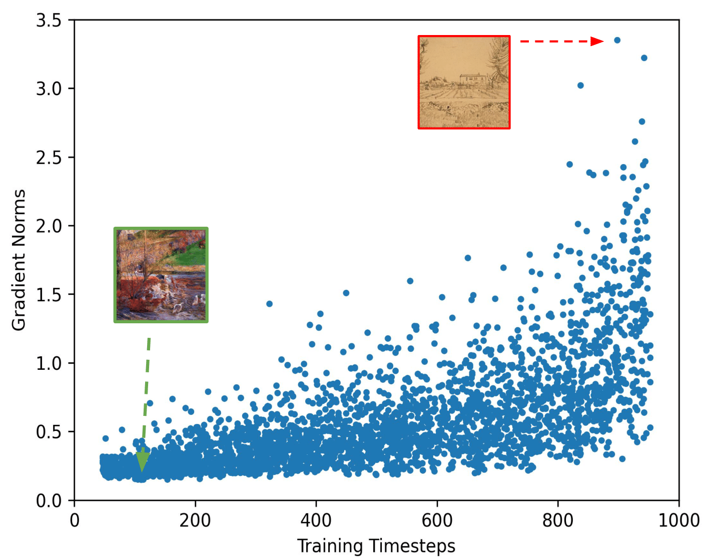
(a) Artbench-2 at checkpoint 100

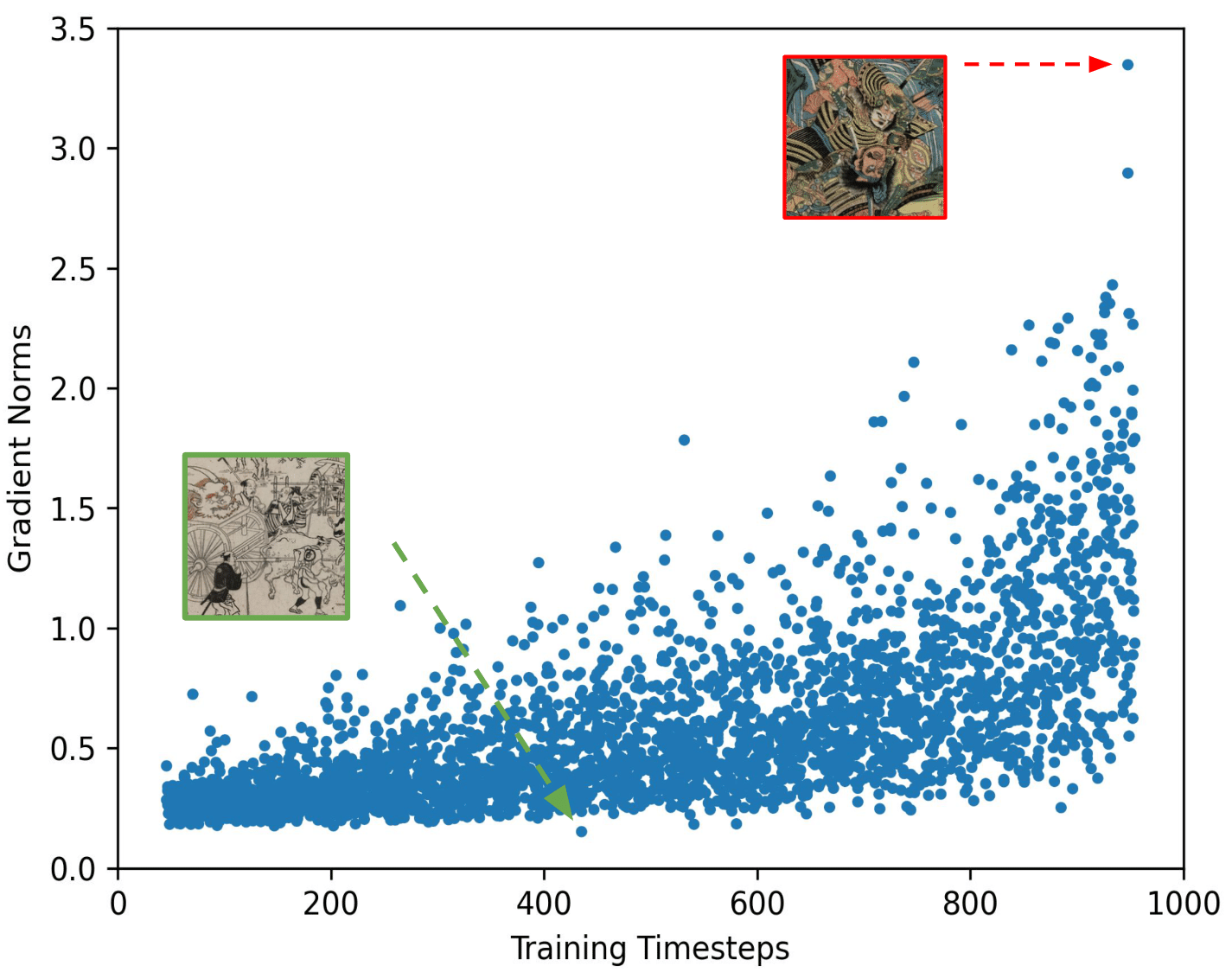
(b) Artbench-2 at checkpoint 200

Figure 1: Samples’ Norm vs. Training Timestep. We plot the norm and timestep of 2,000 randomly selected training samples. We observe that loss gradient norms tend to increase when the training timestep falls in the later range (towards noise). This upward trend is consistent at other checkpoints tested. The sample with the largest norm (red) and smallest norm (green) are shown; no exceptional visual patterns are noticed.

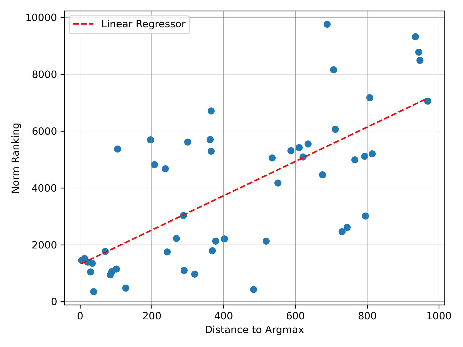
Figure 2: Correlation of Training Timestep and Norm Ranking. We plot the norm ranking and distance between training timestep to $t_{\text{max}}$ for 50 randomly selected samples. The resulting correlation is $0.7$ and the linear regressor (red) has a slope of 6.038.

Varying Timestep for a Single Sample. We further analyze the norm distribution for an individual training sample. At a given model checkpoint, we compute the loss gradient norm for a fixed sample $z$ at every timestep. We plot the norm distribution for randomly selected samples and observe similar trends. Figure 3 shows the distribution for an example training data at three different model stages. The highest norm-inducing region at these three checkpoints all falls within the later timestep range, regardless of where the training timestep is sampled at. The further implication is that for each sample, its loss gradient norm is highly dependent on the chosen timestep. It is also observed that within the same epoch, various samples share similar trends in norm distribution. This suggests a systematic pattern (e.g. artifact of diffusion learning dynamics) beyond individual instances, supporting the intuition that over-reliance on gradient norms may not be ideal.

Timestep Manipulation. We further illustrate the timestep-induced bias by exploring the susceptibility of influence estimation to the manipulation of timesteps. We conduct the experiment on 500 training samples that are characterized by Diffusion-TracIn as “uninfluential” to a random test sample (i.e. influence score is close to 0, neither proponent nor opponent). For each uninfluential sample $z_{i}$, we compute its influence using $t_{\max}(z_{i})$ instead of the original training timestep. The result shows that after deliberately modifying timestep, the ranking of the magnitude of influence for these samples increases by 4,287 positions on average. Given that there are only 10,000 images in the dataset, this notable fluctuation indicates that the timestep-induced bias is significant enough to flip a training sample from uninfluential to proponents or opponents. It further indicates that Diffusion-TracIn’s attribution results could well arise from timestep-induced norms in general. Such findings highlight the potential vulnerability within Diffusion-TracIn as a data attribution method, emphasizing the need for more robust influence estimation techniques.

The preceding sections empirically show that a training sample’s loss gradient norm is highly dependent on timesteps, which produces a consistent trend in norms based on learning dynamics. As the timestep utilized in influence estimation is stochastically sampled in training, instances receive varying degrees of such timestep-induced norm. This bias is particularly evident in samples whose training timestep falls close to $t_{\max}$, leading them to be “generally influential” (Figure 7). These findings suggest samples’ norms are a suboptimal source of information, calling for special attention to the handling of gradient norms.

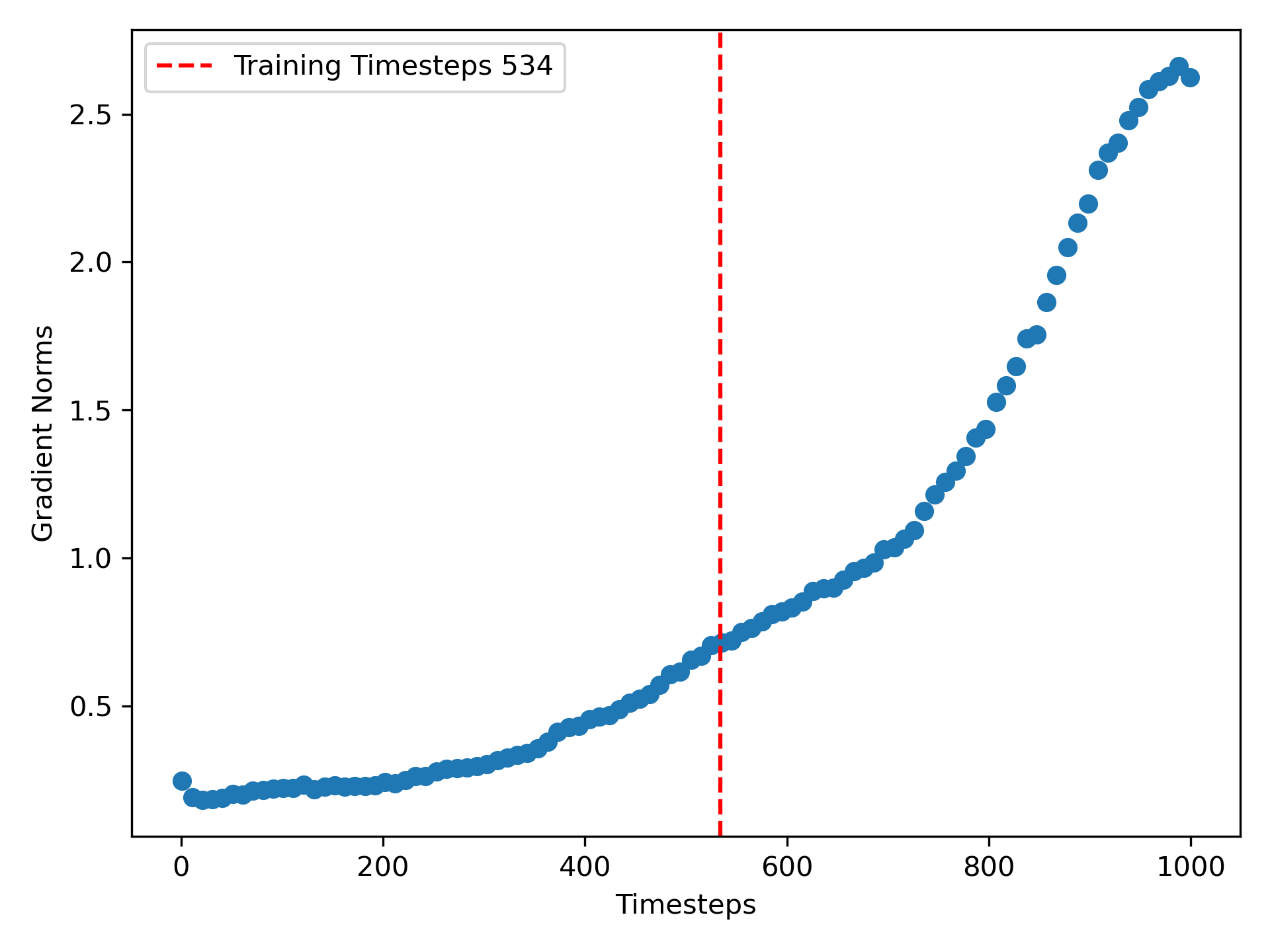
(a) Checkpoint 100

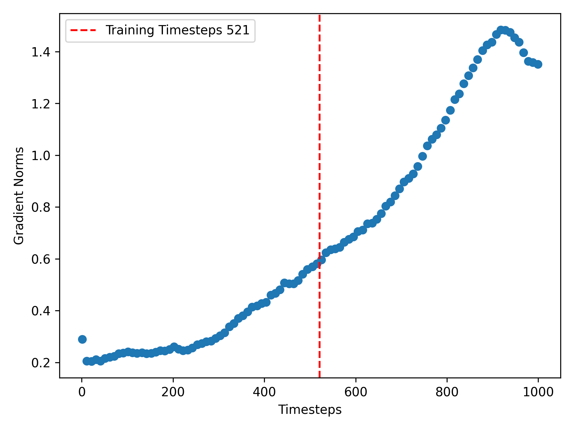
(b) Checkpoint 200

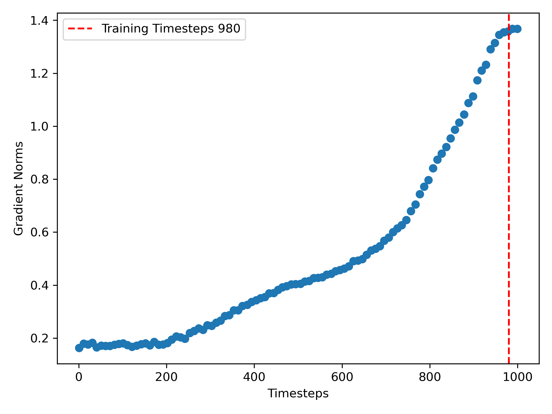
(c) Checkpoint 300

Figure 3: One Sample’s Norms Varying Timestep. Example of norm distributions for one randomly selected sample is shown. On each checkpoint, we observe that the norm distribution is skewed to later timesteps for each individual sample.

5 Method

5.1 Timesteps Sparse Sampling

The extension of TracIn to diffusion models, as formulated in Equation 7, involves an expectation over $T$ timesteps. However, since the number of timesteps can be large (e.g. 1,000) in practice, optimization toward computational efficiency becomes imperative. To address this, we employ a reduced subset of timesteps selected to encapsulate essential information of the sequence. We leverage $n_{t}$ evenly-spaced timesteps $S=\{t_{1},t_{2},...,t_{n_{t}}\}$ ranging from $1$ to $T$ for the test sample $z^{\prime}$ and define

$$\text{Diffusion-TracIn}(z,z^{\prime}):=\sum_{k=1}^{s}\eta_{k}(\frac{1}{{n_{t}}m}\sum_{t\in S}\sum_{i=1}^{m}\nabla_{\theta}L_{t}(\theta_{k},\epsilon_{i},z^{\prime}))\cdot L,$$ (8)

where the timesteps $t_{p}\in S$ approximates the full diffusion trajectory.

5.2 Diffusion-ReTrac

As shown in Section 4.2, the direct application of TracIn to diffusion models leads to a strong dependence on timesteps and the corresponding norm induced for the training sample. The prevalence of this dominating norm effect calls for modification of the approach when applying to diffusion models.

Intuition. By Cauchy-Schwarz inequality, it can be noticed from Equation 4 that

$$|\text{TracIn}(z,z^{\prime})|\leq\sum\eta_{t}\|\nabla\ell(w_{t},z^{\prime})\|\|\nabla\ell(w_{t},z)\|.$$

Hence, training samples with disproportionately large gradient norms tend to have significantly higher influence score $|\text{TracIn}(z,z^{\prime})|$. This suggests that these samples are more likely to be characterized as either a strong proponent or opponent to the given test sample $z^{\prime}$, depending on the direction alignment of $\nabla\ell(w_{t},z^{\prime})$ and $\nabla\ell(w_{t},z)$. As identified in Section 4.2, the loss function component $L_{t}$ from certain timesteps is more likely to have a larger gradient norm. Hence varying degrees of “timestep-induced” norm biases, stemming from systematic learning dynamics, emerge and affect the influence estimations.

Approach. Since the gradient norm is not solely a property attributed to the sample, an ideal instance-based interpretation should not overestimate the influence of samples with large norms and penalize those with small norms.

In fact, this dominating norm effect can be introduced by the choice of timesteps for both test sample $z^{\prime}$ and each training sample $z$, whose loss gradient norms are computed using timestep $t$ and $t_{\text{train}}$ respectively. For test sample $z^{\prime}$, the gradient information $\sum_{t\in S}\sum_{i=1}^{m}\nabla_{\theta}L_{t}(\theta_{k},\epsilon_{i},z^{\prime})$ derives from an expectation over the $n_{t}$ sub-sampled timesteps $S=\{t_{1},\cdots,t_{n_{t}}\}$. Therefore, influence estimation inherently upweights timesteps with larger norms and downweights those with smaller norms. For each training sample $z$, the timestep $t_{\text{train}}$ was stochastically sampled during the training process, hence incorporating varying degrees of timestep-induced norm bias. To this end, we propose Diffusion-ReTrac which introduces normalization that reweights the training samples to address the dominating norm effect. We normalize these two terms and define

$$\text{Diffusion-ReTrac}(z,z^{\prime})=\sum_{k:z_{k}=z}\eta_{k}(\frac{1}{mT}\sum_{t\in S}\sum_{i=1}^{m}\frac{\nabla_{\theta}L_{t}(\theta_{k},z^{\prime},\epsilon_{i})}{\|\nabla_{\theta}L_{t}(\theta_{k},z^{\prime},\epsilon_{i})\|})\cdot\frac{L}{||L||}$$ (9)

The bias introduced to influence estimation due to timestep-induced norms is thus mitigated. In this way, we minimize the vulnerability that the calculated influences are dominated by training samples with a disproportionately large gradient norm arising from stochastic training.

6 Experiments

To interpret model behaviors through training samples, the proposed data attribution method $A$ encompasses two natural perspectives: test-influence $A(z,z^{\prime})$ and self-influence $A(z,z)$. Specifically, test-influence measures the influence of each training sample $z$ on a fixed test sample $z^{\prime}$, entailing a targeted analysis on a specific test sample. On the other hand, self-influence estimates the influence of a training sample on itself, providing rich knowledge about the sample itself and gauges its relative impact on the model’s learning.

We evaluate Diffusion-TracIn and ReTrac under these two objectives. The experiments provide evidence of the dominating norm bias in Diffusion-TracIn influence estimation, presenting instances where this effect may be unnoticed in one objective yet gives rise to substantial failure in another. Our discussion addresses the following questions:

1. Image Tracing: How effective is each method at attributing the learning source of an image to the training data through test-influence?

2. Targeted Attribution: In general, how does Diffusion-ReTrac outperform Diffusion-TracIn by addressing the norm bias?

3. Outlier Detection: Why might the timestep-induced bias be unnoticed in detecting outliers or atypical samples by calculating self-influence?

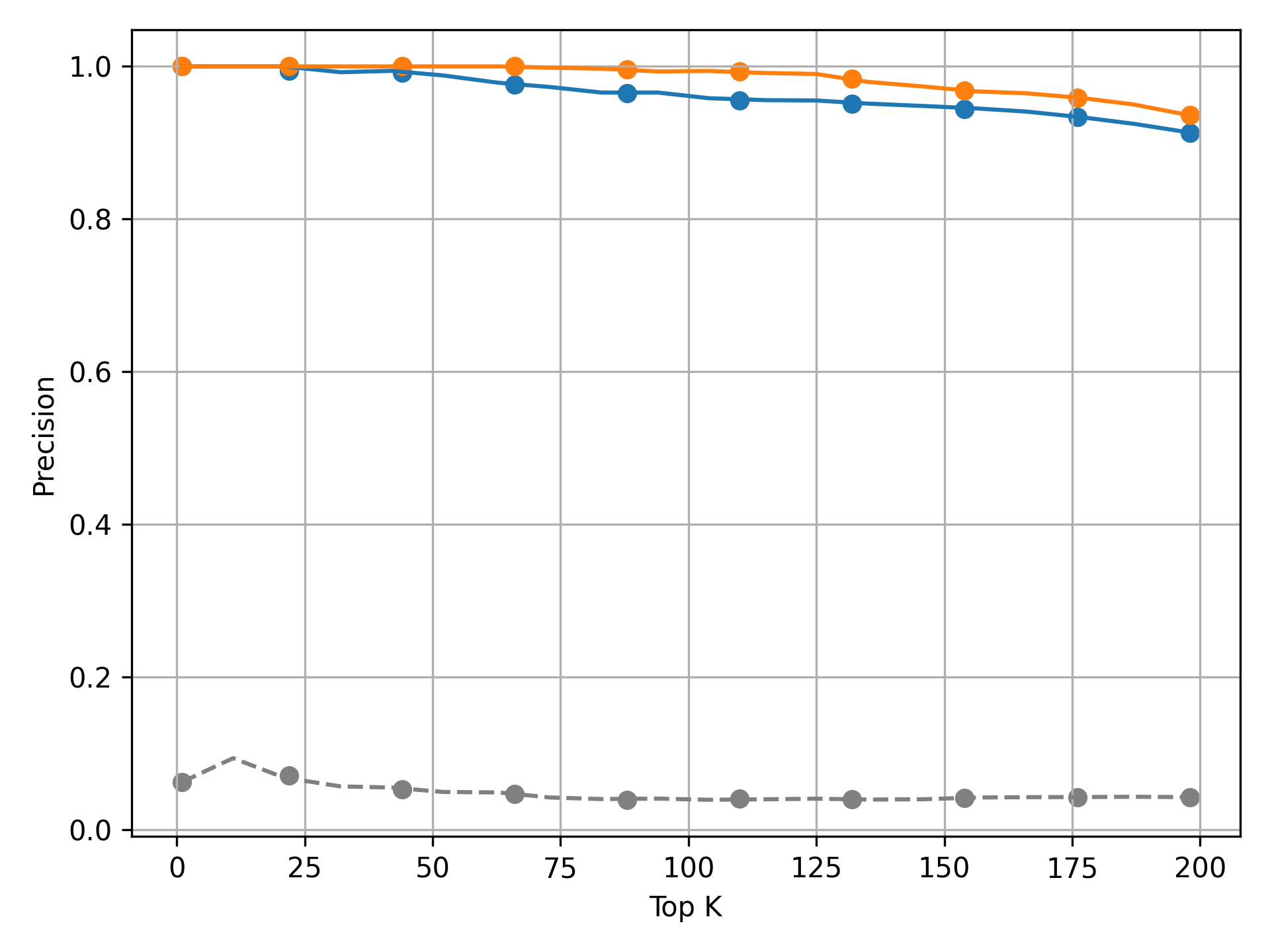
(a) Precision on MNIST zero test samples

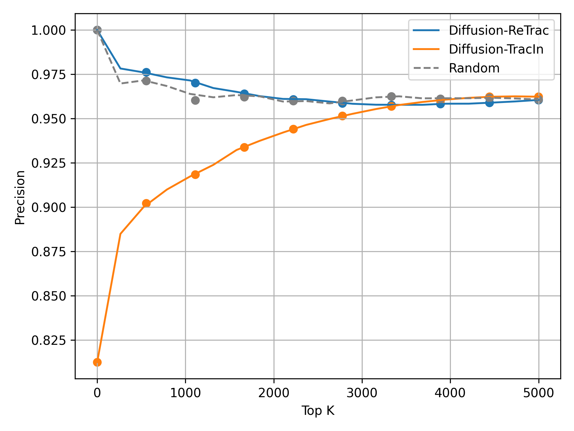
(b) Precision on CIFAR-plane test samples

Figure 4: Image Tracing Accuracy. We measure precision by evaluating the ratio of correctly attributed samples among top $k$ proponents. While (a) shows both methods successfully traced MNIST test samples, (b) shows that Diffusion-TracIn fails to attribute CIFAR-plane test samples since the outlier MNIST samples with large norms are characterized as strong proponents, giving low precision for small $k$. Note that random attribution is a strong baseline in (b) since the 5,000 CIFAR-plane samples are much more likely to be proponents compared to the 200 MNIST samples.

6.1 Image Tracing

One fundamental role of data attribution methods is to trace the model’s outputs back to their origins in the training samples. This idea is also utilized for analyzing memorization [Feldman, 2020], a behavior where the generated sample is attributed to a few nearly identical training samples. In essence, Image source tracing helps pinpoint specific training samples that are responsible for a generation. Thus we evaluate our methods on the question: Given a test sample, which instances in the training dataset is the model’s knowledge of the test sample derived from?

Setup. We extend our experiment using the aforementioned model trained on CIFAR-10 airplane and MNIST zero subclass [Krizhevsky et al., 2009; LeCun and Cortes, 2010]. Given a test sample of MNIST zero, it is expected that the 200 MNIST samples in the training dataset serve as ground truth for the image source. Similarly, a test sample of CIFAR-plane should be attributed to the 5,000 CIFAR training samples. We thus obtain an accuracy score by measuring the correctly attributed proportion among the top-$k$ influential sample.

Results. The precision for Diffusion-TracIn and ReTrac are reported in Figure 4. While both methods successfully attribute the MNIST test samples to the 200 MNIST training samples, Diffusion-TracIn is significantly worse than random baseline in attributing CIFAR-plane test samples. We note that it frequently characterizes MNIST samples as top proponents for CIFAR planes. This aligns with the expectation that Diffusion-TracIn tends to assign higher influence to training samples with large norms, in this case, the outlier MNIST zeros. Further analysis of these influential zeros indicates that their training timestep is sampled exactly at or close to $t_{max}$. This then becomes the confounding factor that further amplifies these outliers’ norms, exacerbating the bias introduced. In contrast, Diffusion-ReTrac successfully attributes both MNIST-zero and CIFAR-plane test samples.

Visualization. Upon closer examining Diffusion-TracIn attribution results, the set of MNIST zero samples exerting influence on plane is relatively consistent across various CIFAR plane test samples. For instance, the MNIST sample with highest influence to the two generated planes are identical in Figure 5. For the CIFAR-plane samples that Diffusion-TracIn successfully attributes (without influential MNIST zeros), there still appear to be generally influential planes. This phenomenon is alleviated for samples retrieved using ReTrac, with sets of influential samples being more distinct and visually intuitive. Additionally, the CIFAR-plane instances with high influence (e.g. among the top $200$) to MNIST test samples tend to be planes with black backgrounds, which to an extent also resemble the MNIST zero. Visualization for these proponent planes is included in Appendix C.2. It is also worth highlighting that Diffusion-ReTrac identifies potentially memorized samples for the generated image, such as the last row in Figure 5.

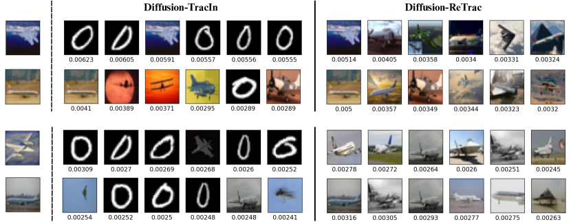
Figure 5: Image Tracing on Outlier Model. We evaluate the two attribution methods on both the training samples (top 2 rows) and generated samples (bottom 2 rows). While both methods successfully attribute MNIST zero test samples, Diffusion-TracIn also incorrectly characterizes MNIST training samples as influential for a CIFAR-plane test sample. This is notably mitigated with Diffusion-ReTrac.

6.2 Targeted Attribution

We then provide a comprehensive analysis of the influential samples retrieved by Diffusion-TracIn and ReTrac. In this experiment, we compute the influence over Artbench-2 and CIFAR-10 datasets. Compared to previous settings, this experiment minimizes the effects of unusually large “sample-induced” gradient norms due to the deliberately introduced outliers. This experiment further compares the capability of Diffusion-TracIn and ReTrac in tasks with different emphases or objectives.

Setup. We compute test-influence on two diffusion models trained with datasets 1). Artbench-2 consisting of “Post-impressionism” and “ukiyo-e” subclasses [Liao et al., 2022; Zheng et al., 2023], each with 5,000 training samples and resolution $64\times 64$, and 2). CIFAR-10  [Krizhevsky et al., 2009] consisting of 50,000 training samples with resolution $32\times 32$.

		Top 10	Top 50	Top 100
ArtBench-2	D-TracIn	0.293	0.261	0.248
	D-ReTrac	0.812	0.646	0.605
CIFAR-10	D-TracIn	0.725	0.663	0.636
	D-ReTrac	0.856	0.800	0.768

Table 1: Targeted Attribution. This table shows the average proportion of unique samples retrieved over 16 test samples. It can be noticed that Diffusion-TracIn overall extracts far less unique samples compared to Diffusion-ReTrac, especially on the two-class ArtBench.

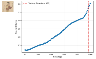
Figure 6: Timestep and Generally Influential. Example of a generally influential sample (left) whose training timestep falls exactly within the $t_{\max}(x)$ region.

Results. To quantify the targeted-ness of the attribution method, we assess the prevalence of generally influential samples. For a list of $n$ random test samples, we analyze the top-$k$ influential samples identified by the two methods, each giving us a total of $n\times k$ samples. Within the set, we report the proportion of distinct instances in Table 1. A lower score implies more overlapping (i.e. generally influential samples). We note that Diffusion-TracIn yields extremely homogenous influential samples. This trend is particularly evident in ArtBench-2, where the two-class setting is less diverse and more prone to bias induced. In this case, Diffusion-TracIn incurs an $\frac{2}{3}$ of overlaps within the top 10 influential samples. This observation aligns with our argument that the stochastically chosen timesteps have amplified the number of samples that exhibit larger gradient norms, therefore causing more generally influential samples.

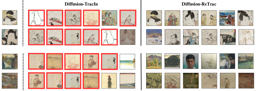
(a) Artbench-2. Top 2 test samples are of the class “Ukiyo-e” and the bottom 2 are of “Post Impressionism”.

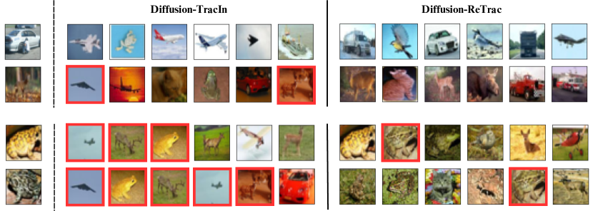
(b) CIFAR-10. Top 2 test samples are of the subclass “automobile,” “deer” and bottom 2 are of “frog”.

Figure 7: Targeted Attribution. We attribute the 8 test samples (leftmost) using both Diffusion-TracIn and Diffusion-ReTrac. The top 6 proponents are shown. The generally influential images that appear multiple times for different test samples are indicated in red. It is visually evident that Diffusion-ReTrac provides more distinct attribution results.

Visualization. From Figure 7, it is visually evident that Diffusion-TracIn retrieves numerous generally influential training samples. The same set of samples exhibits large influences to test samples that are completely different (e.g. in terms of subclass or visual similarities such as color and structure).

Further analysis of these generally influential samples reveals that their associated timestep tends to be close to $t_{\max}$. As an illustration, Figure 6 shows the distribution of norm vs. timestep for an example generally influential instance . This specific sample emerges as influential at checkpoint 80, which coincides with its training timestep falling close to $T_{\text{max}}$. It then becomes generally influential as shown in Figure 7(a) (first proponent on the last row). This phenomenon is notably mitigated after normalization in Diffusion-ReTrac. The revised approach retrieves proponents that bear greater visual resemblance to the test samples, highlighting ReTrac’s targeted attribute and reinforcing that dissimilar test samples are more likely to be influenced by a distinct set of training samples.

6.3 Outlier Detection

Influence estimation is often used to identify outliers that deviate notably from the rest of the training data. Intuitively, outliers independently support the model’s learning at those sparser regions of the input space to which they belong, whereas learning of the typical samples is supported by a wide range of data. Hence in an ideal influence method, outliers tend to exhibit high self-influence, indicating that they exert a high contribution in reducing their own loss. Because of such an outlier-induced norm, we observe that biased estimations may easily go unnoticed in this common metric of outlier detection.

Setup. We begin by training a diffusion model on a combination of the entire 5,000 samples from CIFAR-10 airplane subclass and 200 samples from MNIST zero subclass. Subsequently, we compute the self-influence of each of the training instances, and sort them by descending order. Since the 200 MNIST samples are outliers that independently support a region, we evaluate whether our methods assign high self-influence to the 200 samples of MNIST zero.

Result. The results show that both Diffusion-TracIn and Diffusion-ReTrac successfully rank outlier samples with high self-influence (Table 2). However, the bias introduced by diffusion timesteps is unnoticed in this experiment. Since outliers naturally exhibit larger norms compared to the typical inliers, the timestep-induced norm becomes a more obscure confounding factor and hence is less subtle in the computation of self-influence.

	Top 100	Top 200	Top 300
Diffusion-TracIn	0.880	0.880	1.000
Diffusion-ReTrac	0.860	0.845	1.000

Table 2: Outlier Detection. This table measures the proportion of MNIST samples among top-$k$ identified samples with the highest self-influence. We observe that the performance of these two methods is on par with each other. Both methods assign high self-influence to the 200 MNIST outliers out of the 5,000 CIFAR planes.

Visualization. Examining high-ranking samples shows that the airplane samples with high self-influence (among the top 200) have large contrast and atypical backgrounds compared to airplane samples with low self-influence. Overall, instances with high self-influence tend to exhibit high visual contrast or are difficult to recognize. This observation is consistent with patterns revealed in previous work on influence estimation for VAE [Kong and Chaudhuri, 2021]. Visualization for plane samples with high self-influence is included in Appendix C.1.

7 Conclusion

In this work, we extend data attribution framework to diffusion models and identify a prominent bias in influence estimation originating from loss gradient norms. Our detailed analysis elucidates how this bias propagates into the attribution process, revealing that gradient information harbors undesired bias caused by diffusion model dynamics. Subsequent experiments validate Diffusion-ReTrac as an effective attempt to mitigate this effect, offering fairer and targeted attribution results.

Limitations and future work. A theoretical explanation for the large-norm-inducing timesteps better pinpoints the causes and provides ad hoc solutions for the problem. While renormalization mitigates the dominating norm effect and “generally influential” samples, further examination of the gradient alignments may also be beneficial. Analysis of other potential confounding factors gives further insights into a fair attribution method.

Appendix

A Timestep-Induced Bias

A.1 Norm vs. Timestep

To demonstrate that diffusion timesteps have a significant impact on loss gradient norms, we plot the distribution of 2,000 randomly selected training samples’ norms and their training timesteps. Visualization for the distribution is shown in Figure 8. There is a notable upward trend that peaks at the later range of the timesteps (i.e. timesteps closer to noise), suggesting that samples trained during these later timesteps tend to exhibit larger norms. Additionally, it is also observed that the trend in norm distribution gradually diminishes at the model convergence. This further supports that such variance due to timestep is an artifact of the training dynamic, rather than a property of the training sample. However, Diffusion-TracIn utilizes gradient information throughout the entire learning process instead of focusing solely on those near convergence. This approach is due to the tendency of the latter to contain minimal information, resulting in an inevitable trend in norms affecting influence estimation. This also motivates the renormalization technique in Diffusion-ReTrac.

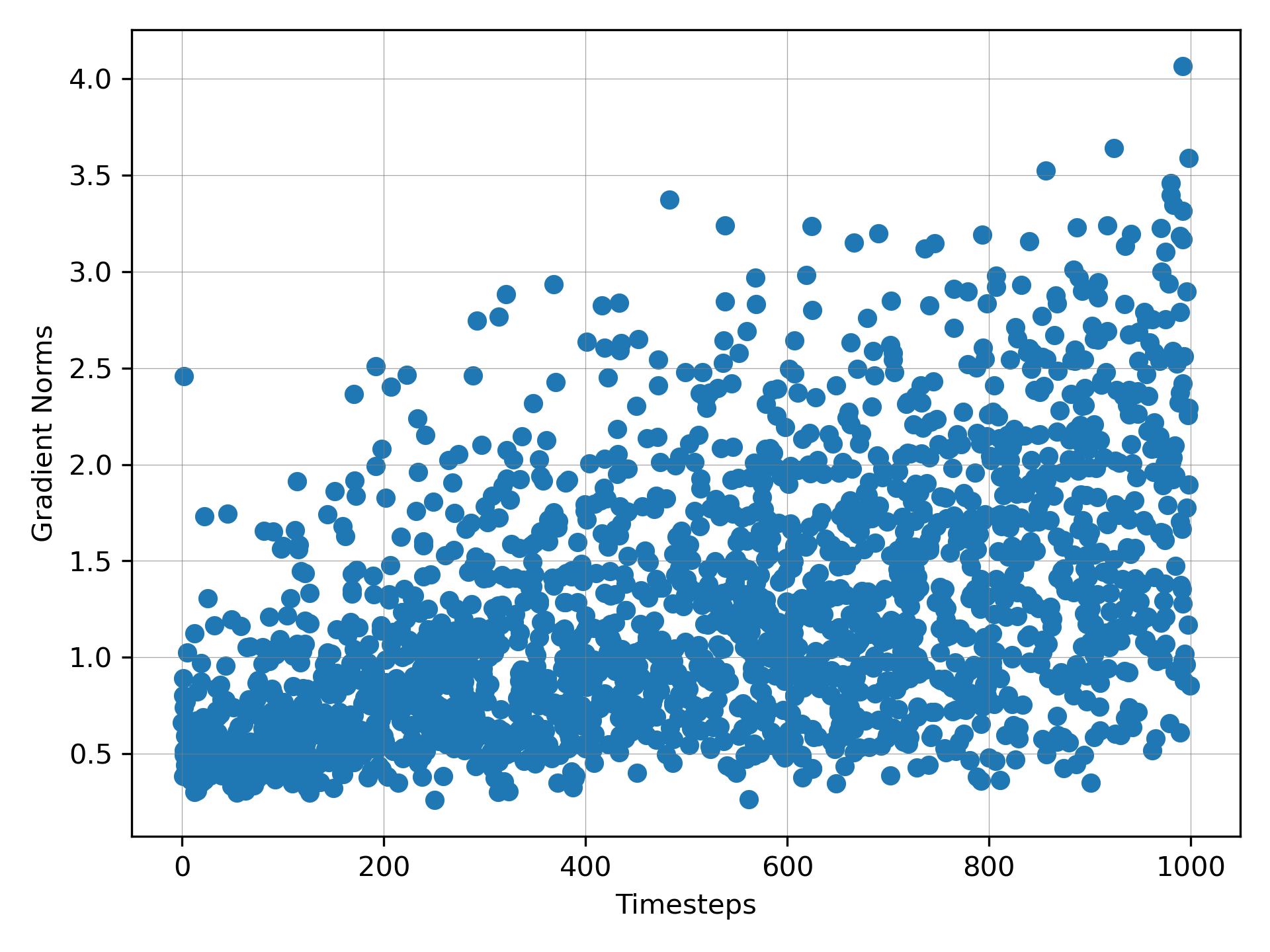
(a) Checkpoint 100

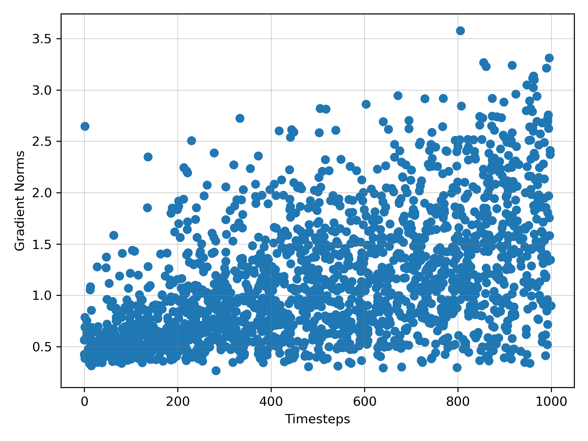
(b) Checkpoint 200

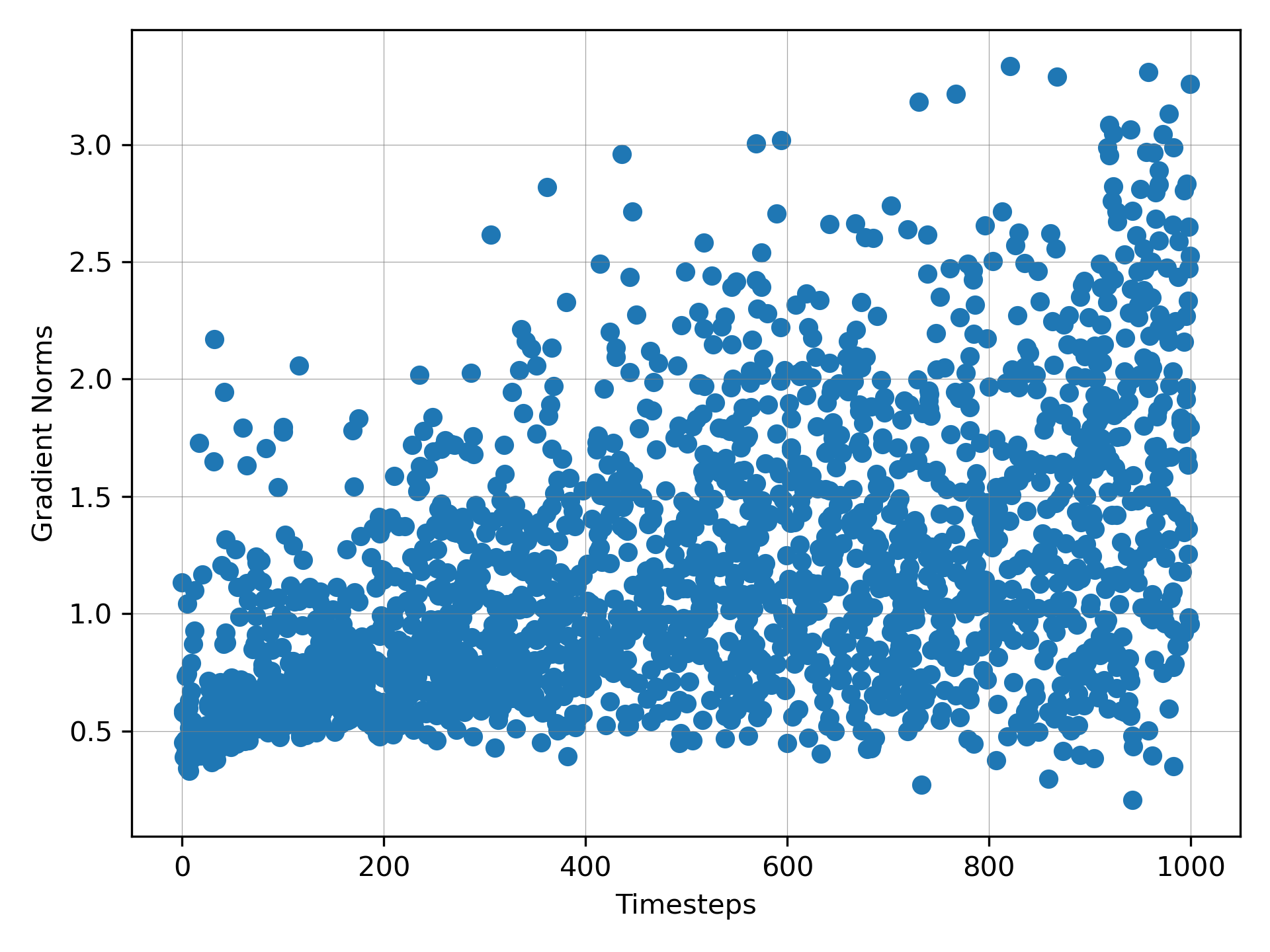
(c) Checkpoint 300

Figure 8: Norm Distribution. We plot the loss gradient norm and training timestep of 2,000 samples. The distributions at checkpoints 100, 200, and 300 all demonstrate an upward trend. This suggests that samples whose training timesteps fall within the later timestep region tend to have a larger norm.

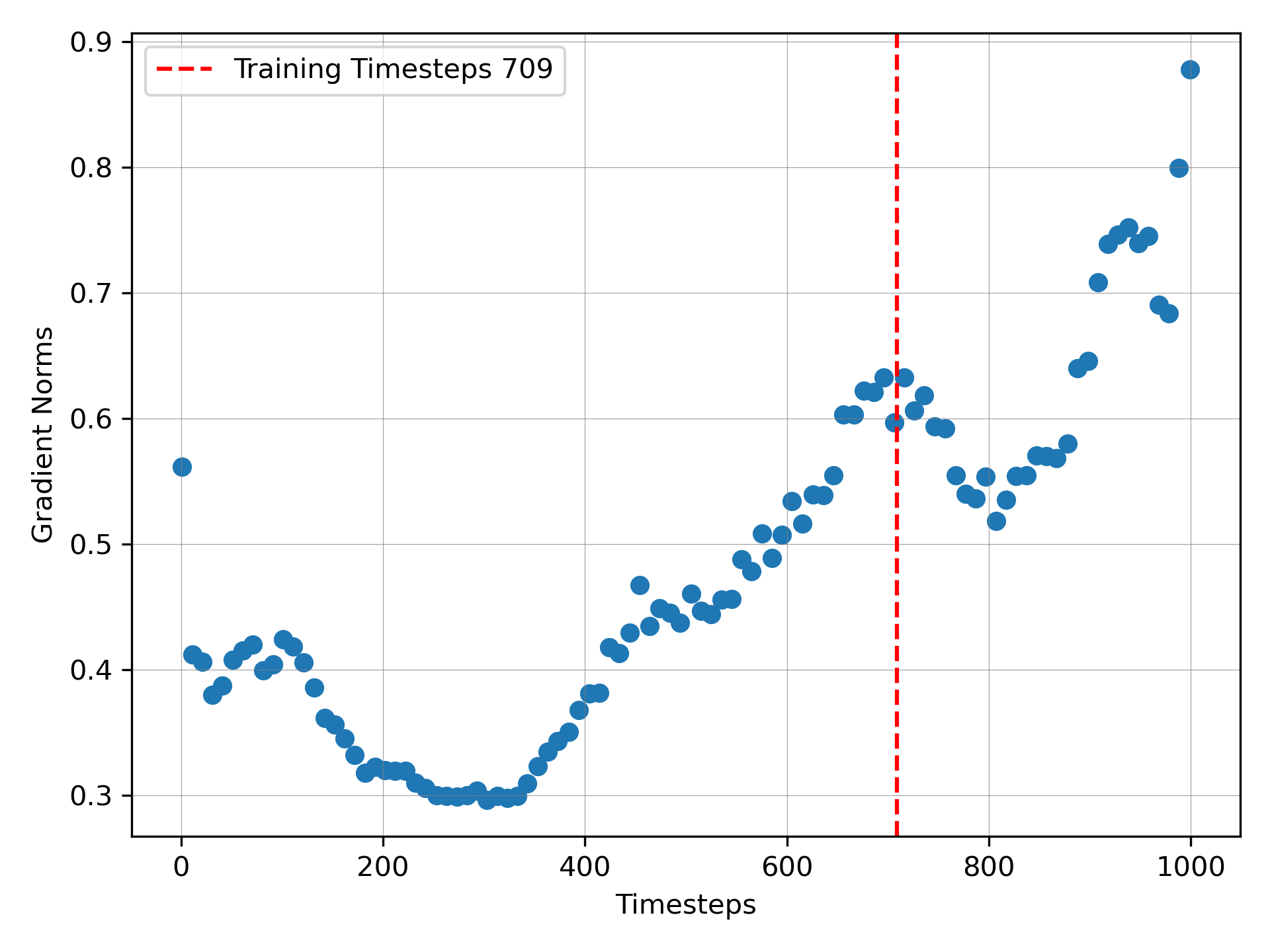
(a) Checkpoint 100

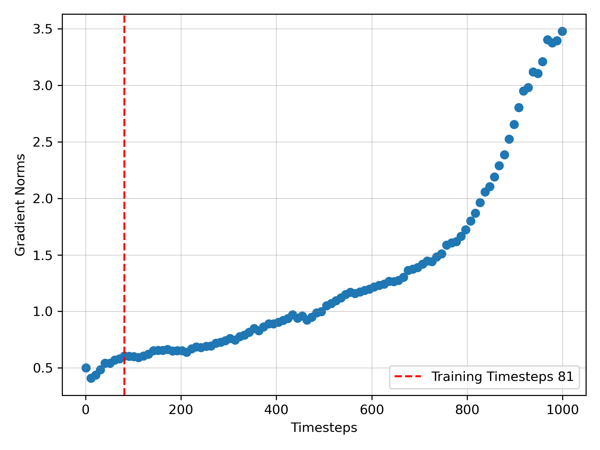
(b) Checkpoint 200

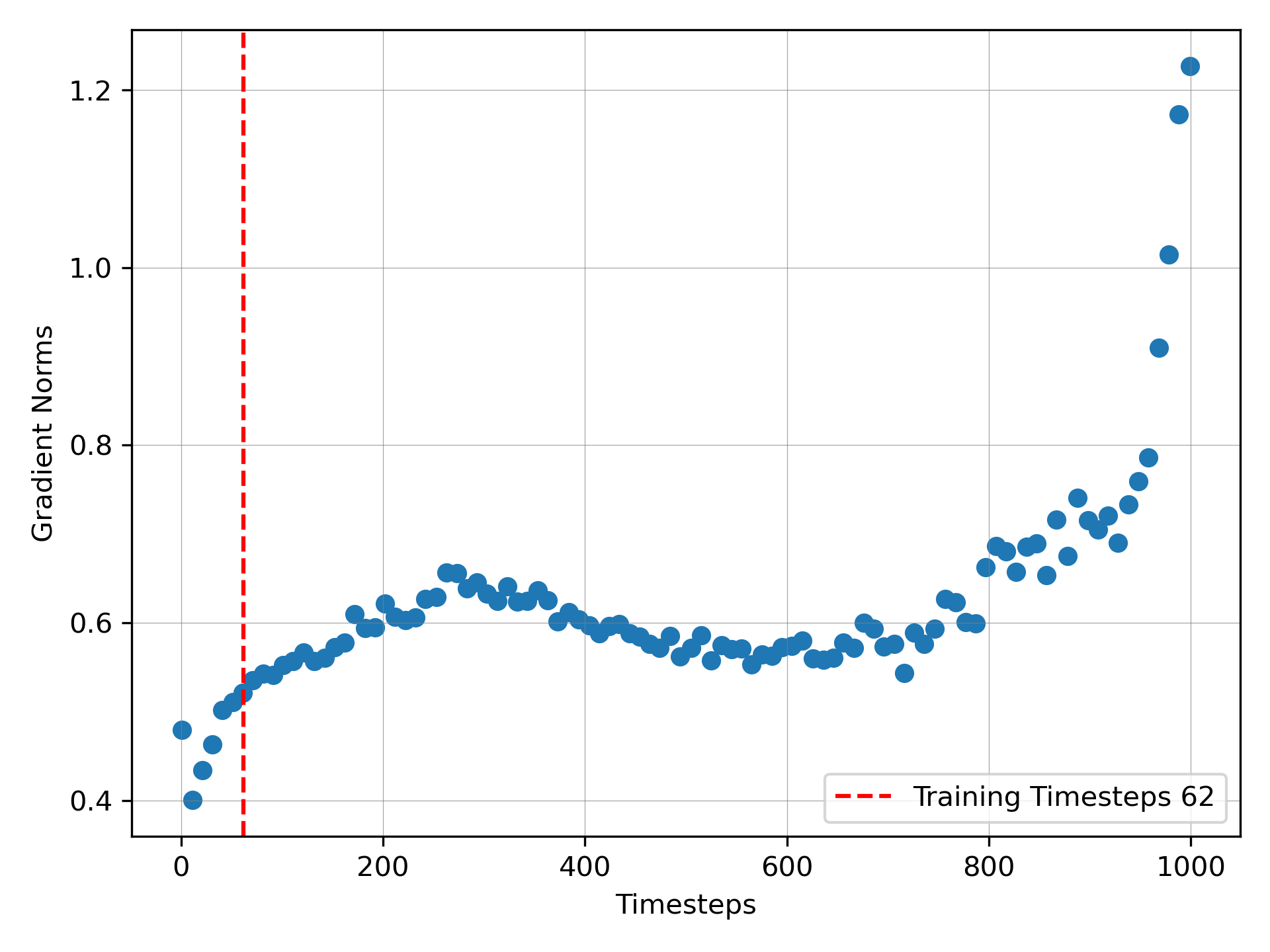
(c) Checkpoint 300

Figure 9: Varying Timestep for a Single Sample. The norms of sample #0 are computed at different timesteps. The distribution obtained at checkpoints 100, 200, and 300 all demonstrates a similar trend that peaks at the later timestep region.

A.2 Varying Timestep for a Single Sample

We further show that for a fixed training sample, the gradient norm with respect to its loss computed at different timesteps varies significantly. This reinforces the effect of training timestep in the estimation of influence, indicating that each sample receives a varying degree of bias since the training timestep is stochastically sampled. An example norm distribution for a fixed sample at different checkpoints is shown in Figure 9.

A.3 Correlation

We provided quantitative analysis addressing the question: If the training timestep of a sample $x$ falls closer to $t_{\max}(x)$, does $x$ also have a relatively larger norm compared to the rest of the training dataset? To analyze the relationship between the stochastically chosen training timestep and the sample’s overall norm ranking among the rest, we obtain a correlation score by i). compute the distance between a sample’s training timesteps $t_{\text{train}}$ and the timestep that yields the maximum norm $t_{\text{max}}(x)$, ii). the ranking of this sample’s gradient norm among all the training samples, and iii). calculate a Spearman Rank correlation score between distance and ranking (Algorithm 1). Figure2 in the main text shows a visualization of the measured correlation.

Algorithm 1 Training Timesteps and Norm Ranking

$y_{1}\leftarrow\{\}$

$y_{2}\leftarrow\{\}$

for $k\leftarrow 0$ to $N$ do:

     $x\leftarrow\text{$k$-th training sample}$

     $y_{1}\leftarrow y_{1}\cup|t_{\max}(x)-t_{\text{train}}(x)|$

     $y_{2}\leftarrow y_{2}\cup\text{Rank}(x)$

end for

return $\text{spearman-rank}(y_{1},y_{2})$

B Generally Influential Samples

As additional motivation for renormalization, we observe that Diffusion-TracIn assigns dominantly high influence to samples with a large norm, even at a single checkpoint. Such a large norm is often associated with training timesteps close to the $t_{\max}$ region, signifying a strong timestep-induced bias in the loss gradient norm. Furthermore, these particular samples only emerge as influential when such checkpoints are utilized, and are likely to persist as strong proponents or opponents throughout the attribution process. This suggests that a substantial norm in one checkpoint can significantly overshadow and dominate attribution results, which is suboptimal if the domination arises from systematic timestep patterns rather than sample-induced variance. However, this phenomenon is notably alleviated after renormalization in Diffusion-ReTrac, providing more consistent and distinct influence estimations.

C Supplemental Visualizations

C.1 CIFAR-Planes with High Self-influence

Self-influence is used to identify outliers in the training dataset. While Diffusion-TracIn and ReTrac assign high self-influence to most of the 200 MNIST samples, certain CIFAR-plane samples also received high self-influence scores and are ranked among the top 200. These plane samples tend to have dark backgrounds or high contrast, which are also visually distinct from typical samples in the CIFAR-plane subclass (Figure 10).

Figure 10: CIFAR-planes with High Self-Influence. These four samples are assigned high self-influence scores by both Diffusion-TracIn and ReTrac. They are visually distinct from the typical plane samples in the training dataset.

C.2 CIFAR-Planes Influential to MNIST Samples

The auxiliary task of Image Source Tracing pinpoints specific training samples that are responsible for the generation of a test sample. For an MNIST zero, while most of the retrieved proponents are MNIST zeros, some planes are also assigned high influences (Figure 11). We noticed that these planes are visually distinct from the other, and visually resemble the MNIST samples. They tend to exhibit a black background and the planes are centered in the middle, which highly resembles the layout of MNIST zeros. This further proves the effectiveness of Diffusion-ReTrac in identifying highly influential samples.

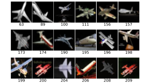
Figure 11: CIFAR-planes Influential to MNIST Samples. These CIFAR-Planes are assigned high influence scores to an MNIST zero test sample. The attribution results are in descending order and the corresponding ranking for each sample is labeled.

D Implementation Details

D.1 Model Details

We trained a Diffusion Denoising Implicit Model (DDIM) [Song et al., 2020] with 1,000 denoising timesteps and 50 inference steps using an Adam optimizer. However, it is noted that our approach should remain consistent across variations of diffusion models, since the methods are designed based on the training process which is largely unaffected by differences in inference procedures. It may also be modified to accommodate the variations in training. Nonetheless, the practical form of TracInCP is expected to remain the same across these variations [Pruthi et al., 2020].

D.2 Checkpoint Selection

When estimating influences, it is ideal to select checkpoints with consistent learning and a steady decline in loss. Checkpoints that are early in the model’s learning stage often yield fluctuating gradient information, while those near model convergence offer limited insights into the attribution. Influence estimation at these early/late epochs of the learning process can introduce noise and compromise the accuracy of attribution results.

Attribution methods that rely on loss gradient norm information are also particularly sensitive to checkpoint selection. We observe that certain samples may exhibit an unusually large norm at specific checkpoints. When this checkpoint is used in Diffusion-TracIn, such samples emerge as generally influential with notably high influence on various test samples, overshadowing attribution results from previous checkpoints. This effect is mitigated in Diffusion-ReTrac due to renormalization, reducing the method’s susceptibility to dominant norms.

D.3 Timestep Selection

To approximate the expectation over timesteps in the attribution efficiently, 50 linearly spaced timesteps over the denoising trajectory are used. This provides similar results to estimating influences across the entire trajectory using $T$ timesteps. It is also observed that the loss induced is relatively stable at neighboring timesteps, while significant variation persists among distant timesteps. This provides justification for reducing computational costs by employing an adequate number of evenly spaced timesteps to approximate the loss over the entire trajectory.

References

- Barshan et al. [2020] Elnaz Barshan, Marc-Etienne Brunet, and Gintare Karolina Dziugaite. Relatif: Identifying explanatory training samples via relative influence. In International Conference on Artificial Intelligence and Statistics, pages 1899–1909. PMLR, 2020.
- Basu et al. [2020] Samyadeep Basu, Philip Pope, and Soheil Feizi. Influence functions in deep learning are fragile. arXiv preprint arXiv:2006.14651, 2020.
- Carlini et al. [2023] Nicolas Carlini, Jamie Hayes, Milad Nasr, Matthew Jagielski, Vikash Sehwag, Florian Tramer, Borja Balle, Daphne Ippolito, and Eric Wallace. Extracting training data from diffusion models. In 32nd USENIX Security Symposium (USENIX Security 23), pages 5253–5270, 2023.
- Dai and Gifford [2023] Zheng Dai and David K Gifford. Training data attribution for diffusion models. arXiv preprint arXiv:2306.02174, 2023.
- Dhariwal and Nichol [2021] Prafulla Dhariwal and Alexander Nichol. Diffusion models beat gans on image synthesis. Advances in neural information processing systems, 34:8780–8794, 2021.
- Feldman [2020] Vitaly Feldman. Does learning require memorization? a short tale about a long tail. In Proceedings of the 52nd Annual ACM SIGACT Symposium on Theory of Computing, pages 954–959, 2020.
- Georgiev et al. [2023] Kristian Georgiev, Joshua Vendrow, Hadi Salman, Sung Min Park, and Aleksander Madry. The journey, not the destination: How data guides diffusion models. 2023.
- Goodfellow et al. [2020] Ian Goodfellow, Jean Pouget-Abadie, Mehdi Mirza, Bing Xu, David Warde-Farley, Sherjil Ozair, Aaron Courville, and Yoshua Bengio. Generative adversarial networks. Communications of the ACM, 63(11):139–144, 2020.
- Hammoudeh and Lowd [2022] Zayd Hammoudeh and Daniel Lowd. Identifying a training-set attack’s target using renormalized influence estimation. In Proceedings of the 2022 ACM SIGSAC Conference on Computer and Communications Security, pages 1367–1381, 2022.
- Hertz et al. [2022] Amir Hertz, Ron Mokady, Jay Tenenbaum, Kfir Aberman, Yael Pritch, and Daniel Cohen-Or. Prompt-to-prompt image editing with cross attention control. arXiv preprint arXiv:2208.01626, 2022.
- Ho and Salimans [2022] Jonathan Ho and Tim Salimans. Classifier-free diffusion guidance. arXiv preprint arXiv:2207.12598, 2022.
- Ho et al. [2020] Jonathan Ho, Ajay Jain, and Pieter Abbeel. Denoising diffusion probabilistic models. Advances in neural information processing systems, 33:6840–6851, 2020.
- Ho et al. [2022] Jonathan Ho, William Chan, Chitwan Saharia, Jay Whang, Ruiqi Gao, Alexey Gritsenko, Diederik P Kingma, Ben Poole, Mohammad Norouzi, David J Fleet, et al. Imagen video: High definition video generation with diffusion models. arXiv preprint arXiv:2210.02303, 2022.
- Khanna et al. [2019] Rajiv Khanna, Been Kim, Joydeep Ghosh, and Sanmi Koyejo. Interpreting black box predictions using fisher kernels. In The 22nd International Conference on Artificial Intelligence and Statistics, pages 3382–3390. PMLR, 2019.
- Kingma and Welling [2013] Diederik P Kingma and Max Welling. Auto-encoding variational bayes. arXiv preprint arXiv:1312.6114, 2013.
- Koh and Liang [2017] Pang Wei Koh and Percy Liang. Understanding black-box predictions via influence functions. In International conference on machine learning, pages 1885–1894. PMLR, 2017.
- Kong et al. [2021] Shuming Kong, Yanyan Shen, and Linpeng Huang. Resolving training biases via influence-based data relabeling. In International Conference on Learning Representations, 2021.
- Kong and Chaudhuri [2021] Zhifeng Kong and Kamalika Chaudhuri. Understanding instance-based interpretability of variational auto-encoders. Advances in Neural Information Processing Systems, 34:2400–2412, 2021.
- Kong et al. [2020] Zhifeng Kong, Wei Ping, Jiaji Huang, Kexin Zhao, and Bryan Catanzaro. Diffwave: A versatile diffusion model for audio synthesis. arXiv preprint arXiv:2009.09761, 2020.
- Krizhevsky et al. [2009] Alex Krizhevsky, Geoffrey Hinton, et al. Learning multiple layers of features from tiny images. 2009.
- LeCun and Cortes [2010] Yann LeCun and Corinna Cortes. MNIST handwritten digit database. 2010. URL http://yann.lecun.com/exdb/mnist/.
- Li et al. [2022] Xiang Li, John Thickstun, Ishaan Gulrajani, Percy S Liang, and Tatsunori B Hashimoto. Diffusion-lm improves controllable text generation. Advances in Neural Information Processing Systems, 35:4328–4343, 2022.
- Liao et al. [2022] Peiyuan Liao, Xiuyu Li, Xihui Liu, and Kurt Keutzer. The artbench dataset: Benchmarking generative models with artworks. arXiv preprint arXiv:2206.11404, 2022.
- Lin et al. [2022] Jinkun Lin, Anqi Zhang, Mathias Lécuyer, Jinyang Li, Aurojit Panda, and Siddhartha Sen. Measuring the effect of training data on deep learning predictions via randomized experiments. In International Conference on Machine Learning, pages 13468–13504. PMLR, 2022.
- Liu et al. [2021] Zhuoming Liu, Hao Ding, Huaping Zhong, Weijia Li, Jifeng Dai, and Conghui He. Influence selection for active learning. In Proceedings of the IEEE/CVF International Conference on Computer Vision, pages 9274–9283, 2021.
- Park et al. [2023] Sung Min Park, Kristian Georgiev, Andrew Ilyas, Guillaume Leclerc, and Aleksander Madry. Trak: Attributing model behavior at scale. arXiv preprint arXiv:2303.14186, 2023.
- Pruthi et al. [2020] Garima Pruthi, Frederick Liu, Satyen Kale, and Mukund Sundararajan. Estimating training data influence by tracing gradient descent. Advances in Neural Information Processing Systems, 33:19920–19930, 2020.
- Rombach et al. [2022] Robin Rombach, Andreas Blattmann, Dominik Lorenz, Patrick Esser, and Björn Ommer. High-resolution image synthesis with latent diffusion models. In Proceedings of the IEEE/CVF conference on computer vision and pattern recognition, pages 10684–10695, 2022.
- Saharia et al. [2022] Chitwan Saharia, William Chan, Huiwen Chang, Chris Lee, Jonathan Ho, Tim Salimans, David Fleet, and Mohammad Norouzi. Palette: Image-to-image diffusion models. In ACM SIGGRAPH 2022 Conference Proceedings, pages 1–10, 2022.
- Somepalli et al. [2023] Gowthami Somepalli, Vasu Singla, Micah Goldblum, Jonas Geiping, and Tom Goldstein. Diffusion art or digital forgery? investigating data replication in diffusion models. In Proceedings of the IEEE/CVF Conference on Computer Vision and Pattern Recognition, pages 6048–6058, 2023.
- Song et al. [2020] Jiaming Song, Chenlin Meng, and Stefano Ermon. Denoising diffusion implicit models. arXiv preprint arXiv:2010.02502, 2020.
- Terashita et al. [2021] Naoyuki Terashita, Hiroki Ohashi, Yuichi Nonaka, and Takashi Kanemaru. Influence estimation for generative adversarial networks. arXiv preprint arXiv:2101.08367, 2021.
- van den Burg and Williams [2021] Gerrit van den Burg and Chris Williams. On memorization in probabilistic deep generative models. Advances in Neural Information Processing Systems, 34:27916–27928, 2021.
- Yeh et al. [2018] Chih-Kuan Yeh, Joon Kim, Ian En-Hsu Yen, and Pradeep K Ravikumar. Representer point selection for explaining deep neural networks. Advances in neural information processing systems, 31, 2018.
- Zhang et al. [2023] Lvmin Zhang, Anyi Rao, and Maneesh Agrawala. Adding conditional control to text-to-image diffusion models. In Proceedings of the IEEE/CVF International Conference on Computer Vision, pages 3836–3847, 2023.
- Zheng et al. [2023] Xiaosen Zheng, Tianyu Pang, Chao Du, Jing Jiang, and Min Lin. Intriguing properties of data attribution on diffusion models. arXiv preprint arXiv:2311.00500, 2023.