Supplement to: A Novel Interpretable Fusion Analytic Framework for Investigating Functional Brain Connectivity Differences in Cognitive Impairments
Jeong-Jae Kim
Graduate Program in Cognitive Science, Yonsei University, Seoul, Republic of Korea
These authors contributed equally to this work
Yeseul Jeon
Department of Statistics and Data Science, Yonsei University, Seoul, Republic of Korea
These authors contributed equally to this work
SuMin Yu
Department of Psychology and Neuroscience, Duke University, Durham, North Carolina, USA
Junggu Choi
Graduate Program in Cognitive Science, Yonsei University, Seoul, Republic of Korea
Sanghoon Han
Graduate Program in Cognitive Science, Yonsei University, Seoul, Republic of Korea
Department of Psychology, Yonsei University, Seoul, Republic of Korea
Corresponding author : sanghoon.han@yonsei.ac.kr
Abstract
Functional magnetic resonance imaging (fMRI) data is characterized by its complexity and high–dimensionality, encompassing signals from various regions of interests (ROIs) that exhibit intricate correlations. Analyzing fMRI data directly proves challenging due to its intricate structure. Nevertheless, ROIs convey crucial information about brain activities through their connections, offering insights into distinctive brain activity characteristics between different groups. To address this, we propose a cutting-edge interpretable fusion analytic framework that facilitates the identification and understanding of ROI connectivity disparities between two groups, thereby revealing their unique features. Our novel approach encompasses three key steps. Firstly, we construct ROI functional connectivity networks (FCNs) to effectively manage fMRI data. Secondly, employing the FCNs, we utilize a self–attention deep learning model for binary classification, generating an attention distribution that encodes group differences. Lastly, we employ a latent space item-response model to extract group representative ROI features, visualizing these features on the group summary FCNs. We validate the effectiveness of our framework by analyzing four types of cognitive impairments, showcasing its capability to identify significant ROIs contributing to the differences between the two disease groups. This novel interpretable fusion analytic framework holds immense potential for advancing our understanding of cognitive impairments and could pave the way for more targeted therapeutic interventions.
Supplementary Figures and Tables
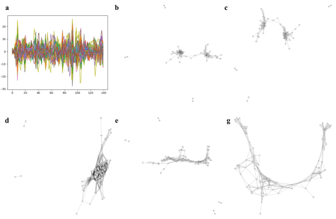
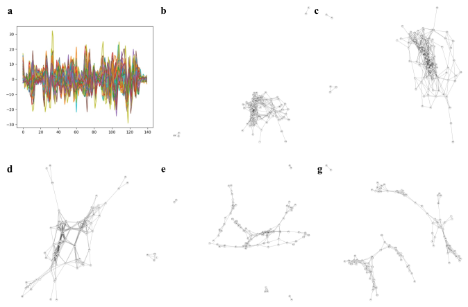
Supplementary Figure 1: Correlation coefficient based FCNs and dimension reduction based FCNs of MCI subject. (a) illustrates the ROIs, rs-fMRI BOLD signals for a sample of subjects with MCI. These FCN graphs were generated using various approaches. Firstly, we employed correlation-based methods such as Pearson’s r or Fisher’s z values (shown in (b) and (c) to establish intricate and interconnected FCNs. However, comprehending the specific attributes of each brain region within these correlation-based FCNs proved challenging. To gain a deeper understanding of the interrelationships between brain regions, we employed dimension reduction techniques to estimate the latent positions of the brain regions. (d) demonstrates the brain region patterns embedded in a 2D space with the highest exploratory power, obtained through PCA in linear space. Additionally, we utilized t-SNE (stochastic space-based FCN) as shown in (e), which assumes that the patterns between brain regions follow a specific probability distribution and learns the degree of similarity between these distributions. Furthermore, we employed UMAP (topological space-based FCN) depicted in (f) to capture the topological similarity of the waveform patterns generated by the ROIs.Supplementary Figure 2: Correlation coefficient based FCNs and dimension reduction based FCNs of EMCI subject. (a) illustrates the ROIs, rs-fMRI BOLD signals for a sample of subjects with EMCI. These FCN graphs were generated using various approaches. Firstly, we employed correlation-based methods such as Pearson’s r or Fisher’s z values (shown in (b) and (c) to establish intricate and interconnected FCNs. However, comprehending the specific attributes of each brain region within these correlation-based FCNs proved challenging. To gain a deeper understanding of the interrelationships between brain regions, we employed dimension reduction techniques to estimate the latent positions of the brain regions. (d) demonstrates the brain region patterns embedded in a 2D space with the highest exploratory power, obtained through PCA in linear space. Additionally, we utilized t-SNE (stochastic space-based FCN) as shown in (e), which assumes that the patterns between brain regions follow a specific probability distribution and learns the degree of similarity between these distributions. Furthermore, we employed UMAP (topological space-based FCN) depicted in (f) to capture the topological similarity of the waveform patterns generated by the ROIs.Supplementary Figure 3: Correlation coefficient based FCNs and dimension reduction based FCNs of LMCI subject. (a) illustrates the ROIs, rs-fMRI BOLD signals for a sample of subjects with LMCI. These FCN graphs were generated using various approaches. Firstly, we employed correlation-based methods such as Pearson’s r or Fisher’s z values (shown in (b) and (c) to establish intricate and interconnected FCNs. However, comprehending the specific attributes of each brain region within these correlation-based FCNs proved challenging. To gain a deeper understanding of the interrelationships between brain regions, we employed dimension reduction techniques to estimate the latent positions of the brain regions. (d) demonstrates the brain region patterns embedded in a 2D space with the highest exploratory power, obtained through PCA in linear space. Additionally, we utilized t-SNE (stochastic space-based FCN) as shown in (e), which assumes that the patterns between brain regions follow a specific probability distribution and learns the degree of similarity between these distributions. Furthermore, we employed UMAP (topological space-based FCN) depicted in (f) to capture the topological similarity of the waveform patterns generated by the ROIs.
Supplementary Table 2: Top 25% ROIs that show distribution differences between disease group pairs.
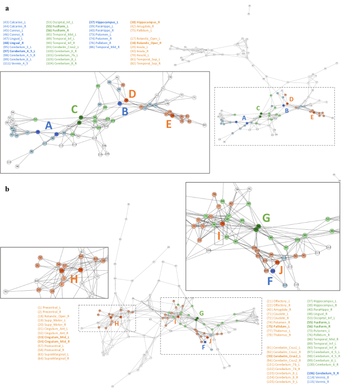
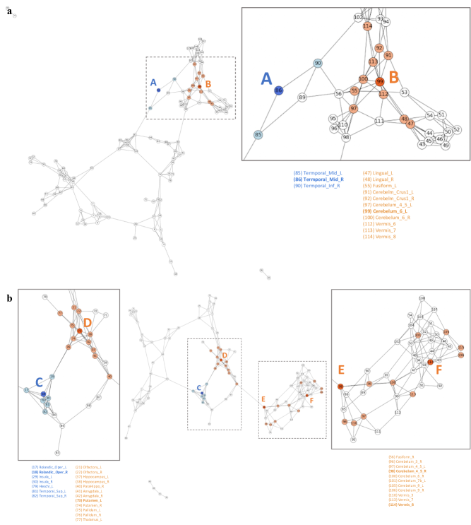
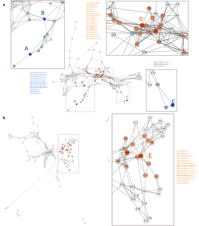
Figure 4: (a) AD group summary FCN and (b) EMCI group summary FCN. The darker saturation colors indicates meaningful ROIs of each group using LSIRM and ROI nodes which are directly connected to this meaningful ROIs are represented by the same color with a lower brightness level. Here D, E, H, I, and J indicate clusters that exhibit more pronounced responses in the respective group than in the comparative group (orange colored cluster), with C and G representing clusters responsive in both diseases (green colored cluster), while A, B, and F signifies a cluster responsive solely in one group (blue colored cluster).Figure 5: (a) AD group summary FCN and (b) LMCI group summary FCN. The darker saturation colors indicates meaningful ROIs of each group using LSIRM and ROI nodes which are directly connected to this meaningful ROIs are represented by the same color with a lower brightness level. Here B, D, E, and F indicate clusters that exhibit more pronounced responses in the respective group than in the comparative group (orange colored cluster), while A and C signifies a cluster responsive solely in one group (blue colored cluster).Figure 6: (a) EMCI group summary FCN and (b) LMCI group summary FCN. The darker saturation colors indicates meaningful ROIs of each group using LSIRM and ROI nodes which are directly connected to this meaningful ROIs are represented by the same color with a lower brightness level. Here the orange colored cluster D and E indicate clusters that exhibit more pronounced responses in the respective group than in the comparative group, while A, B and C signifies a cluster responsive solely in EMCI and not in LMCI.