Whither or wither the Sulfur Anomaly in Planetary Nebulae?

Abstract

We present a thorough investigation of the long standing sulfur anomaly enigma. Our analysis uses chemical abundances from the most extensive dataset available for 126 planetary nebulae (PNe) with improved accuracy and reduced uncertainties from a $10\times 10$ degree Galactic bulge region. By using argon as a superior PNe metallicity indicator, the anomaly is significantly reduced and better constrained. For the first time in PNe we show sulfur $\alpha$-element lock-step with both oxygen and argon. We dispel hypotheses that the anomaly originates from underestimation of higher sulfur ionization stages. Using a machine learning approach, we show that earlier ionization correction factor (ICFs) schemes contributed significantly to the anomaly. We find a correlation between the sulfur anomaly and the age/mass of PNe progenitors, with the anomaly either absent or significantly reduced in PNe with young progenitors. Despite inherent challenges and uncertainties, we link this to PNe dust chemistry, noting those with carbon-dust chemistry show a more pronounced anomaly. By integrating these findings, we provide a plausible explanation for the residual, reduced sulfur anomaly and propose its potential as an indicator of relative galaxy age compositions based on PNe.

1 Introduction

Sulfur, as an $\alpha$ element, should be produced in lockstep with others like oxygen, neon, argon, and chlorine in more massive stars, so its cosmic abundance should also be proportional. Strong correlations between sulfur and oxygen abundances are seen in H ii regions and blue compact galaxies. However, historically, Planetary Nebula (PNe hereafter) sulfur abundances, which arise from low-to-intermediate mass progenitors, have consistently been lower, giving rise to the so-called “sulfur anomaly” first identified in PNe by Henry et al. (2004).

Extensive efforts to explain the PNe sulfur anomaly through observational and theoretical approaches has so far proved elusive. One suggestion is past failure to properly account for the abundances of unseen ionization stages above S²⁺. Another factor is the difference in evolutionary stages in H ii regions, blue compact galaxies and PNe. H ii regions are the current sites of chemical enrichment, from which the next generation of stars emerge. In contrast, PNe form a highly diverse and complex family, with progenitor masses spanning from $\sim$8 $M_{\odot}$ to 1 $M_{\odot}$ and so exhibiting a wide range of ages, from tens of millions of years to over 10 Gigayears.

Shingles & Karakas (2013) looked at whether the s-process is responsible for destroying sulfur during late stage stellar evolution but their study did not support this. Another idea is dust depletion of sulfur (Henry et al., 2012; García-Hernández & Górny, 2014). Delgado-Inglada et al. (2015) suggested oxygen and neon may be enriched during PN progenitor evolution which could give more scatter, depending on progenitor mass (and so effectively age). As a result they consider argon and chlorine more reliable metalicity indicators. Given difficulties in measuring weak chlorine lines, argon is by far the easier to work with and is adopted here.

1.1 The context of the sulphur anomaly

Our Galaxy is an ideal testing ground for refining chemical evolutionary models. Galactic H ii regions represent zero-age systems while PNe represent older to considerably older populations of intermediate- to low-mass stars for study. For PNe the observed abundances can deviate to sub- and super-solar depending on progenitor age. PNe allow accurate determination of abundances among various chemical tracers through their emission lines, including precise abundance measurements of alpha elements. These elements, created by massive stars, remain unaltered by their progenitors and reflect molecular cloud composition when the stars were formed. If $\alpha$ elements like oxygen, neon, sulfur, and argon are produced in lockstep in massive stars, their abundances should exhibit equivalent correlations. H ii region and PNe observations have revealed strong correlations between oxygen and neon. They are considered indicators of their formation environments. Similar lockstep behaviour has been noted for argon. However, previous sulfur abundance studies in Galactic disk PNe, e.g. (Henry et al., 2004) and (Henry et al., 2012), and Galactic Bulge PNe by (Cavichia et al., 2010), report data points that considerably deviate from the narrow, linear tracks for H ii regions. Instead they exhibit a broad spread in sulfur abundances that generally fall lower than for H ii regions. This discrepancy is the sulphur anomaly. It has been discussed in detail by e.g. Henry et al. (2004) and Henry et al. (2012) and has been based on O/H values as the metalicity indicator.

We examined steps from previous studies that derived PNe sulfur abundances from their spectra. These directly determine the ionic abundances of S⁺ and S²⁺, when observable, and then multiplied by an “ionisation correction factor” (ICF) e.g. (Mathis, 1985; Delgado-Inglada et al., 2014), calculated to account for unobserved ionisation stages. Possible reasons given for the sulfur anomaly include underestimation of higher ionisation stages when using these ICFs (see later). Henry et al. (2012) tested the sulfur abundance deficit across a range of nebular properties but found no strong correlations. Recently, by studying the born-again nebula V4334 Sgr and using ESO VLT spectroscopic observations from 2006 to 2022, Reichel et al. (2022) confirmed an [S iii] level, contrary to expectation of a decrease, because the S²⁺ stage, if it dominates, will rapidly recombine to S⁺. A possible explanation is recharge from underestimated fractions of higher ionisation stages. They propose this could explain the anomaly but this object is itself anomalous and only a single data point.

2 ESO VLT FORS2 Spectroscopy

Our new catalogue of abundances for Galactic bulge PNe from quality VLT/FORS2 spectra, Tan et al. (2024) (Paper III) provides the most comprehensive and reliable PNe abundances available to re-examine the sulfur anomaly. We found the first clear example of a lock-step relation for argon and neon with oxygen unlike previous studies, reflecting a reduction in our data’s error dispersion. We re-examined this lockstep behaviour and the relationship between sulfur and oxygen abundances using our high S/N data from the same telescope and instrument and for a well-defined PNe sample. We use these new data to investigate the sulfur anomaly. Our PNe selection was based on likely Galactic bulge membership, as detailed in Paper I (Tan et al., 2023).

To derive abundances, we used the Fitzpatrick (1999) extinction law to account for interstellar reddening. We used the ICF scheme in Delgado-Inglada et al. (2014), hereafter DMS14, to correct for unobserved sulfur ionisation stages. This is a key difference to previous work, e.g. Kingsburgh & Barlow (1994) and Kwitter & Henry (2001), hereafter KW01, as used by HSK12. We derive S/H and O/H values for 124 objects on the standard 12 + $\log$(X/H) scale, yielding high-quality results and $<0.2$ dex uncertainties.

3 The sulfur anomaly and a comparison with literature studies

Fig. 1 shows the relationship between S/H and O/H for 162 Galactic disk PNe from Henry et al. (2012), hereafter HSK12, and the 124 PNe in our ESO VLT bulge sample. HSK12 incorporates data from Henry et al. (2004), Milingo et al. (2010), and Henry et al. (2010), which adopt the Kwitter & Henry (2001) ICF scheme.

As proposed by Delgado-Inglada et al. (2015), AGB star evolution may modify nebular oxygen abundances compared to their progenitors. Their analysis suggested using Ar/H or Cl/H as a more reliable metalicity indicator. Given the large uncertainties associated with Cl/H derivation, we adopt Ar/H. In Fig. 1 we plot S/H against Ar/H. We include data for H ii regions in the nearby spiral galaxy M101 from Kennicutt Jr et al. (2003) and metal-poor blue compact galaxies from Izotov & Thuan (1999) (collectively hereafter H2BCG), where the $\alpha$-element lockstep behaviour is demonstrated. We exclude data from H ii regions with an uncertainty in $\log$(S/O) $>0.1$ dex, as they exhibit a noticeable deviation from the main H2BCG data. Table 1 presents best-fit parameters for S/H versus O/H and Ar/H of each sample from linear least-squares regression using scipy.stats.linregress, together with Pearson’s correlation coefficients ($r$).

The left-most panel of Fig. 1 presents the non-lockstep behaviour of S/H versus O/H for Galactic disk PNe from HSK12 (as blue and purple data points) as two trends: a sparsely populated (13%) upper trend that aligns with the H2BCG data (green points), and a well-populated (87%) locus below the H2BCG trend encapsulating the anomaly. The slope of the best fit line (in blue) significantly deviates from unity with a formal $R^{2}=0.26$, providing the main anomaly locus.

We calculate the sulfur deficit, $d$(S), as the discrepancy between the predicted $12+\log$(S/H) values (from the best-fit line for $12+\log$(S/H) versus $12+\log$(O/H) of H2BCG) and the actual observed PNe values, following HSK12. Using only results in HSK12 with reported measurement uncertainty $<0.2$ dex (denoted as HSK12+), the median $d$(S) is $-0.40^{+0.31}_{-0.29}$ dex. The sulfur deficit seen in the S/H versus O/H plot is at least partially due to the ICF scheme used as we show in the next section.

The middle-left plot of Fig. 1 is the equivalent S/H versus Ar/H plot. Here, there is only a single, broad locus of PNe data points falling below but closer to the H2BCG line. This shows that using the O/H metallicity indicator is a key factor in the sulfur anomaly in HSK12. The data scatter in the left panels may reflect uncertainties in determining reliable PNe chemical abundances using low-resolution spectroscopic observations on 2-m telescopes. Our Paper III shows that literature results based on low-resolution spectra from 2-m telescopes generally show a deviation $>0.1$ dex from those from the VLT observations for the $\alpha$ elements.

In the right panels of Fig. 1, we show Galactic bulge PNe data from Paper III that displays a broader metalicity range, with many objects having super-solar O/H and Ar/H. Compared to HSK12, our high-quality VLT/FORS2 abundances show less scatter with most points on a narrower track below the H2BCG trend. The bulge PNe show clear lockstep behaviour for S/H versus O/H with a strong correlation coefficient of $r=0.84$. The best-fit line has a near unity slope. This is the first time lockstep behaviour between S/H and O/H has been shown for any PNe sample. The S deficit is a smaller systematic offset of $\sim 0.2$ dex, with a median $d$(S) of $0.24_{-0.18}^{+0.27}$ dex. The scatter at the sub-solar O/H remains significant. The sulfur lockstep behaviour is further tightened in S/H versus Ar/H, as in the right-most panel of Fig. 1. These are our major new findings.

We reanalysed the HSK12 chemical abundances using their de-reddened line intensities following methods described in Paper III. Our recalculated values show median differences compared to HSK12 for S/H and O/H of 0.1 and $-0.07$ dex, respectively, while agreeing within the measurement uncertainty for Ar/H. These discrepancies could be attributed to the differences in atomic datasets and ICF schemes used. As a result of our recalculations, the median $d$(S) reported in HSK12 and shown in Figure 2 would be halved to $0.19_{-0.27}^{+0.24}$ dex.

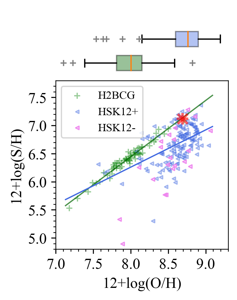
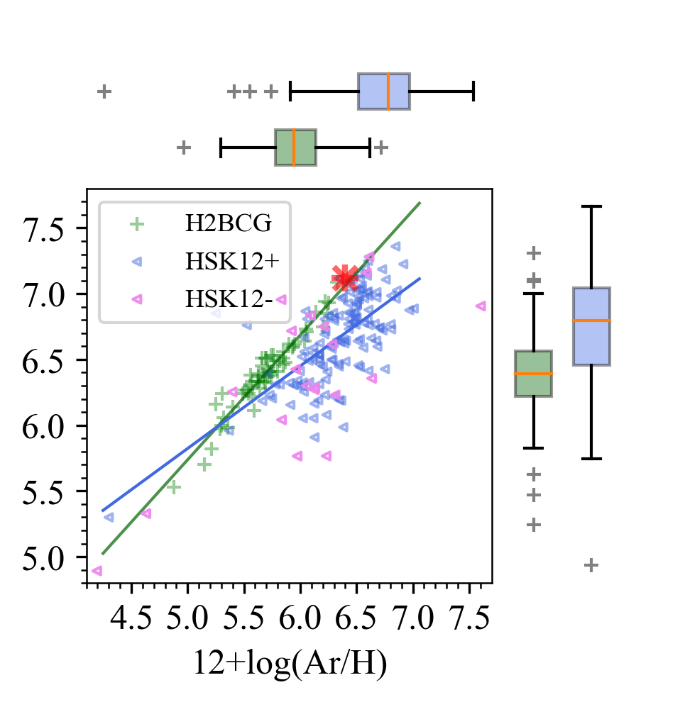
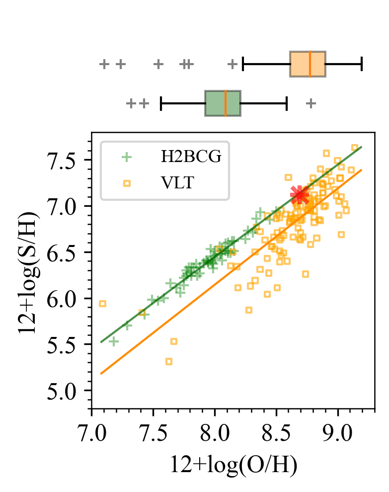
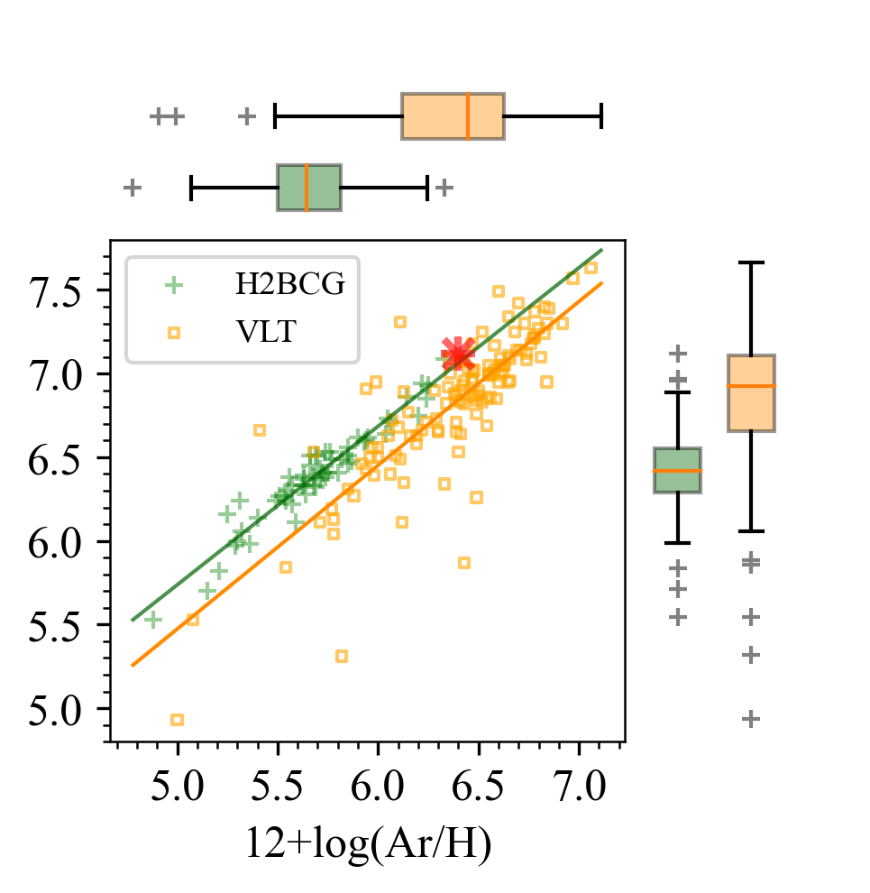
Figure 1: Comparison of S/H versus O/H and Ar/H among PNe samples c.f. H2BCG data (green crosses). The two left panels show Galactic disk PNe from HKS12, with blue and pink triangles triangles for high and lower quality measurements with uncertainties $<0.2$ dex and $>0.2$ dex. The right two panels give our Galactic bulge PNe results from Paper III as orange squares. In all panels, best-fit lines are the same color as the data. Only HSK12 data points with uncertainties $<0.2$ dex (HSK12+) were fitted. Our VLT results for O/H and Ar/H display best-fit lines parallel to the H2BCG trends with clear lock-step behaviour. The red asterisk is solar abundance. Color-coded boxplots at the top and right of each panel depict distributions of O/H, Ar/H and S/H. Red lines indicate median values with boxes extending from the 25th to 75th percentiles and whiskers from 1% to 99% with outliers as crosses.

2*Sample	2*X/H vs. S/H	S/H from ICF scheme					S/H from ML
		slope	$-$intercept	$R^{2}$	$r$		slope	$-$intercept	$R^{2}$	$r$
VLT [124]	O	1.05$\pm$0.06	$-$2.22$\pm$0.53	0.71	0.84		0.99$\pm$0.06	$-$1.70$\pm$0.51$-$	0.70	0.84
	Ar	0.98$\pm$0.06	$-$0.58$\pm$0.38	0.69	0.83		0.95$\pm$0.06	0.75$\pm$0.38	0.70	0.83
HSK12+ [140]	O	0.66$\pm$0.10	$-$0.96$\pm$0.82	0.26	0.51		0.78$\pm$0.11	$-$0.02$\pm$0.93$-$	0.29	0.54
	Ar	0.63$\pm$0.06	$-$2.69$\pm$0.38	0.44	0.67		0.70$\pm$0.07	2.31$\pm$0.44	0.44	0.67
H2BCG [61]	O	1.00$\pm$0.03	$-$1.56$\pm$0.21	0.96	0.98		-	-	-	-
	Ar	0.95$\pm$0.04	$-$1.00$\pm$0.21	0.92	0.96		-	-	-	-

Table 1: Slope, intercept , corresponding errors, and the coefficient of determination ($R^{2}$) from the least-squares regression for the $12+\log$(S/H) versus both $12+\log$(O/H) and $12+\log$(Ar/H) data, along with correlation coefficients ($r$) for Galactic disk PNe from HSK12+ and bulge PNe from Paper III, as shown in Fig. 1. The best-fit parameters derived with S/H from the literature ICF schemes are presented in cols. 3-6 while those obtained with S/H from machine learning-derived icf(S) are presented in cols. 7-10. The final two rows presents results for H2BCG.

4 Understanding the sulfur anomaly

We examine the sulfur anomaly in Galactic disk and bulge PNe samples. Despite a notable reduction in the S/H deficit found in our high-quality bulge PNe data, the sulfur anomaly persists for some PNe. We focus on potential artificial causes of this anomaly, including underestimation of sulfur higher ionization stages beyond S²⁺ in photoionization models. We implement a machine learning approach to derive an ad hoc sulfur ICF for each object to examine the ICF scheme proposed in the literature. We compare our optical observations with infrared literature results where higher ionisation stages could be directly observed, to examine possible issues associated with use of optical observations.

4.1 Validation of ICF scheme via machine learning

The KW01 and DMS14 ICF literature formulae were obtained through analytical fitting to photoionization models. The sulfur anomaly has been attributed to failure to properly account for high ionisation stages through use of an incorrect ICF for sulfur in HSK12, something our re-calculations of their data confirm. Sabin et al. (2022) first introduced machine learning (ML) techniques to determine ICFs tailored to individual PNe. Here, we apply ML to a large sample. To minimise uncertainties with the ICF formulae, we adopt a random forest (RF) regressor (Breiman, 2001) (a learning method based on decision tree regression), to predict ICF values (S/(S⁺+S²⁺) or S/S⁺). RF input features include He²⁺/He⁺, O²⁺/O⁺, S²⁺/S⁺, Ar³⁺/Ar²⁺, and Cl³⁺/Cl²⁺. We used the RandomForestRegressor in the Python library Scikit-Learn (Pedregosa et al., 2011). Objects with unobserved O²⁺ were excluded due to large O/H uncertainties and challenges in accurately determining the O²⁺/O⁺ ratio. Where other ionic stages in input features were not seen, such as Ar³⁺ or Cl³⁺, a separate RF regressor predicted the ionic fraction ratios (e.g., Ar³⁺/Ar²⁺ and Cl³⁺/Cl²⁺) using He²⁺/He⁺ and O²⁺/O⁺ as input features.

An extensive photoionization model grid of PNe was computed as in Delgado-Inglada et al. (2014). We selected PNe photoionization models from an extended grid version with a larger effective temperature range for PNe central stars. These models were run with version c17.01 of Cloudy (Ferland et al., 2017) and hold in the 3MdB_17 database (Morisset et al., 2015) under the reference PNe_2020. From the $>700,000$ models we chose $\sim 120,000$ that met realistic PN model selection criteria in Delgado-Inglada et al. (2014) to train the RF regressor. The full sample was divided into a training set (75% of the sample), a validation set (12.5%), and a test set (12.5%). The training set trained the RF regressor and the validation set tuned the hyperparameter $\alpha$ of the RF regressor to enhance efficiency and accuracy achieved via a grid-search cross-validation (CV) of $\alpha$ values (see Appendix B).

Figure 2 displays the distribution of differences between the $12+\log$(S/H) values obtained using the icf(S) from literature-based ICF schemes and our ML approach for the PNe sample in HSK12+ and Paper III. The median differences for these samples are $-0.04_{-0.24}^{+0.13}$ and $-0.0006^{+0.15}_{-0.15}$ dex. The ICF scheme in DMS14, applied in Paper III, shows no systematic difference and smaller discrepancies to the ML values, unlike the KW01 used in HSK12. The ML comparison for HSK12+ (right panel of Figure 2) has a left-skewed distribution, suggesting underestimation of S/H and, consequently, a slightly larger average sulfur deficit of $\sim$0.07 dex. The best-fit line parameters for ML S/H values are presented in Table 1 for both HSK12+ and Paper III PNe samples. The higher $R^{2}$ and $r$ values indicate a better linear relationship, while the best-fit line for HSK12+ is closer to unity. Considering the sulfur anomaly typically exceeds 0.1 dex, the inaccuracies linked to the ICF schemes are likely not the only cause of the sulfur anomaly. The increased consistency between the ICF scheme in DMS14 and the ML results shows that the DMS14 scheme is more reliable, supporting the argument that their ICF scheme reduces the sulfur anomaly, as shown here.

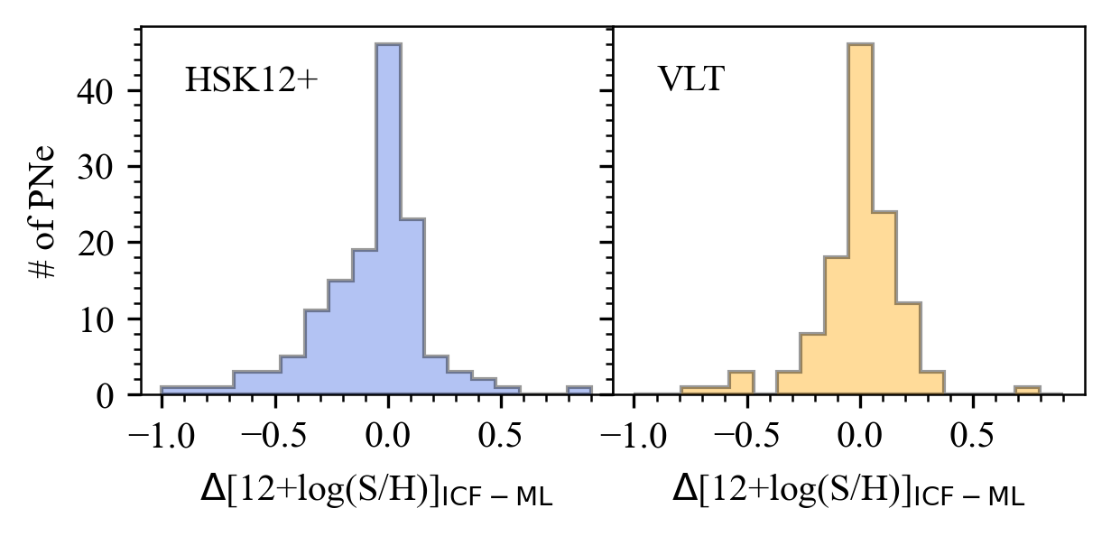
Figure 2: Differences between $12+\log$(S/H) values from literature ICF formulae and our machine learning approach. The HSK12+ sample in the left panel adopted the KW01 ICF scheme, while the right panel presents PNe from Paper III using the DMS14 ICF scheme. The left-skewed distribution in the HSK12+ panel suggests a contribution to the sulfur anomaly from the KW01 ICF scheme.

4.2 Mid-infrared observations of PNe

The S/H deficiency seen in Galactic PNe is suggested as due to underestimation of higher ionization stages of sulfur in photoionization models, e.g. Henry et al. (2012); Reichel et al. (2022). S/H values from mid-infrared Spitzer spectra in Pottasch & Bernard-Salas (2015), PBS15 hereafter, enables observation of the higher ionization stage S³⁺ and are systematically higher than our results, with a median difference of 0.17 dex. The left panel of Fig. 3 shows the VLT S/H versus O/H plot for eight bulge PNe in common with PBS15. The VLT results show the sulphur anomaly in terms of the H2BCG linear fit with an $R^{2}$ of 0.34. The PBS15 O/H values are from optical observations but our VLT spectra are superior. The right panel shows good agreement between PBS15 sulfur abundances from mid-infrared spectra and oxygen abundances from our VLT spectra. We find $R^{2}=0.71$, consistent with the H2BCG results. A comparison of our sulfur ionic abundances and PBS15 shows that the S²⁺/H⁺ mid-infrared values from [S iii] $\lambda$18.7 $\mu m$ and $\lambda$36.5 $\mu m$ in PBS15 are systematically higher than from the equivalent optical [S iii] $\lambda$6312 line, with a median difference of 0.16 dex. The two outliers in the right hand plot in Fig. 3 have no lower S²⁺/H⁺ values from mid-infrared spectra. The dashed green line is the H2BCG fit and the red asterisk is solar abundance. For 6/8 PNe in common the mid-infrared S/H values follow the expected trend line. Comparison of our icf(S) and S/(S⁺+S²⁺) or S/S⁺ in PBS15 shows a median difference of $\sim$4%, with underestimation $>$10% in only two PNe.

Hence, the sulfur anomaly is unlikely to arise from underestimation of higher sulfur ionization stages in the photoionization model and their ICFs. Optical measurement of [S iii] lines gives lower S²⁺ abundances compared to their mid-infrared counterparts, if the values of S²⁺ inferred from the mid-infrared are more accurate.

Figure 3: Comparison of S/H versus O/H for 8 bulge PNe in common with Pottasch & Bernard-Salas (2015). The left panel shows S/H values from optical VLT observations in Paper III. The right panel gives S/H values inferred from PBS15 mid-infrared data. The dashed green line is the fit to the H2BCG data; the red asterisk denotes the solar abundance. For 6 out of 8 PNe in common the mid-infrared S/H values essentially follow the expected trend line.

We highlight some issues associated with mixing the optical and mid-infrared data for chemical abundance derivation. First, Appendix.A gives the same plots for neon and argon as for sulfur in Fig. 3. Our Paper III VLT results show good agreement with the H2BCG data, while the mid-infrared data yields systematically higher results by 0.29 and 0.33 dex for neon and argon. A similar issue with neon abundance was reported in Dors Jr et al. (2013) when studying star-forming regions. This was partly attributed to abundance variations across the nebulae. It is possible mid-infrared and optical data intrinsically provide different abundance estimates, with the mid-infrared data yielding higher estimates. This is supported by detailed PNe photoionization modelling in Bandyopadhyay et al. (2021) and dusty PNe photoionization modelling in Otsuka et al. (2017), where best-fit photoionization models for the optical emission lines and PNe physical conditions yielded lower fluxes of [S iii] $\lambda$18.7 $\mu$m and $\lambda$36.5 $\mu$m than the observed mid-infrared line fluxes.

4.3 Underestimation of S²⁺/H⁺from optical spectra

To address the potential underestimation of S²⁺ ionic abundances using optical spectra that could lead to a discrepancy between optical and mid-infrared observations, we re-examined our Paper III S/H measurements. We considered several factors, including errors in interstellar correction at the red [S iii] lines from the use of a single, standard extinction law that may not be valid in the Galactic bulge (Gould et al., 2001; Udalski, 2003), uncertainties in [S iii] line flux measurements and the varying spatial distribution of sulfur and oxygen in PNe.

To quantify the impact of interstellar extinction correction uncertainties, we recalculated S/H using emission line lists from Paper III and compared two extinction laws introduced in Howarth (1983) and Cardelli et al. (1989), with that of Fitzpatrick (1999) used in Paper III. We showed good agreement between the S²⁺/H⁺ and S/O abundance ratios derived using the Howarth (1983) and Fitzpatrick (1999) extinction laws, with a median difference of $-0.001^{+0.004}_{-0.006}$ dex and $-0.00\pm 0.007$ dex. The extinction law of Cardelli et al. (1989) yielded slightly lower values, indicating even lower results compared to the mid-infrared, with median differences in S²⁺/H⁺ and $\log$(S/O) of $-0.07^{+0.04}_{-0.06}$ and $-0.03\pm 0.03$ dex. We find the extinction correction impact on the sulfur anomaly is insignificant compared to the discrepancy between optical and mid-infrared S²⁺ results and conclude that the extinction correction is not a contributing factor to the anomaly.

Our Paper III VLT data covered a wavelength range up to 8500 Å, which only allowed detection of the [S iii] $\lambda$6312 line. We investigated whether lower signal-to-noise ratios for the [S iii] $\lambda$6312 line might lead to underestimation of its line fluxes. Our analysis showed that the sulfur anomaly size had no correlation with measured raw fluxes of the [S iii] $\lambda$6312 line, indicating that the sulfur deficiency is not due to weak line fluxes.

The near-IR [S iii] $\lambda\lambda$9069, 9531 lines were not observed in our VLT spectra. The ionization structure of the PNe may introduce uncertainties in the S²⁺ abundance determinations due the absence of electron temperatures derived from [S iii] line ratios, as S²⁺ (22.34–34.79 eV) probes lower ionization zones than O²⁺ (35.12-54.94 eV). While the analysis of H ii regions utilising deep spectra in Freeman et al. (2013) suggests no such systematic difference between T_e([S iii]) and T_e([O iii]), the ionising sources and the gas and dust components in H ii regions are considerably different from PNe. A comprehensive exploration of high-quality PNe data with the near-IR [S iii] line observations, where the telluric contamination can be satisfactorily removed, is imperative to examine how the ionization structures of PNe affect the sulfur deficit.

Abundances from long-slit spectroscopy only sample a portion of a PN often weighted towards high-ionization regions near the central star (Ali et al., 2016). Hence, we also consider literature on PNe integral field unit (IFU) spectroscopy. Such 2-D spectroscopy can provide global abundance data. Using ionic abundances of O and S derived from IFU observations, the sulfur anomaly persists for four PNe in Ali et al. (2016) and three PNe in García-Rojas et al. (2022). For most objects, the sulfur deficit reduced by 0.10 to 0.34 dex; however, two PNe show a greater $d$(S) by $\sim 0.12$ dex using IFU observations. Thus, ionization stratification and spatial variation in sulfur and oxygen abundances within a PN may partly account for the observed sulfur anomaly.

To conclude, firstly HKS12 and Paper III employ a non-biased ICF for sulfur, as shown by our ML icf(S) values. Secondly, possible intrinsic differences between optical and mid-infrared spectroscopy results may lead to higher abundances derived from mid-infrared spectra. Thirdly, among the application of different extinction laws, uncertainties in measuring weak [S iii] $\lambda$6312 lines and any abundance inhomogeneities within the PNe, none appear to have a significant impact that could lead to underestimation of S²⁺ ionic abundances. The PNe sulfur anomaly, though reduced in our work, remains a genuine effect but is unlikely to arise from underestimating sulfur ionization stages above S²⁺.

5 The sulfur deficit across different PNe samples and properties

After confirming in Section 4 that the sulfur anomaly is a real, albeit much reduced in PNe, it is likely that the varying PNe S/H deficiencies in different Galactic regions, as discussed in Section 3, could indicate a progenitor population effect. Below we present an analysis of the sulfur deficit considering links to PN progenitor age/mass, dust chemistry and Galactic location. The results are summarised in Fig. 4 and explored in terms of PNe progenitor age and sulfur deficit.

5.1 PNe progenitor ages/masses

We developed a basic PNe age estimator based on our high-quality VLT abundances as detailed in Appendix C. We differentiate between young ($t_{\star}<1$ Gyr) and old ($t_{\star}>7.5$ Gyr) PN populations by combining the Peimbert classes with an extant scheme in Stanghellini & Haywood (2018) that establish a link between the effectiveness of nitrogen production in PN progenitors and their ages/masses. We used this criteria to divide the HSK12+ disk sample and our VLT bulge sample into crude young and old progenitor star PNe populations.

In Fig. 4, we give a combined plot for sulfur deficit, $d$(S), as a function of Galactic height in kpc; 12 + $\log$(O/H) and histograms of $d$(S) values with bins of 0.11 dex for the HSK12+ disk PNe sample (top row) and VLT bulge PNe sample (bottom row). We color-coded the data according to these crude ages.

In the upper left panel of Fig. 4, the HSK12+ disk PNe show a broad spread in $d$(S) with a peak at $\sim 0.4$. The old PNe population is restricted to a narrower range of higher $d$(S), while the younger population have a broader distribution from $1.0$ to $-0.6$ dex in $d$(S). Objects with no sulfur deficit primarily have young progenitors. In the lower left panel of Fig. 4, the bulge PNe sample has a narrower uni-modal $d$(S) distribution peaking at $\sim 0.3$ dex. The old population is restricted to a narrower range of higher $d$(S) while the younger population dominates at lower $d$(S) values up to $-0.2$ dex.

A two-sample Kolmogorov–Smirnov (KS) test (Smirnov, 1939) using scipy.stats.ks_2samp compared the $d$(S) distribution of the young and old populations. The KS p-values are 8E-4 for disk PNe and only 1E-5 for bulge PNe. Adopting a stringent significance level $\alpha$ of 0.001, we reject the null hypothesis that the $d$(S) of different age groups come from the same population.

Given the crudeness of the age classification these results are indicative, but they imply the sulfur deficit is PN age related and hence to the initial progenitor mass.

5.2 Galactic height from the mid-plane

We use identifications of central stars of Galactic PNe from Gaia EDR3 in Chornay & Walton (2021) (CW21) and González-Santamaría et al. (2021) (GSM21) and their parallax distances, to determine Galactic heights from the mid-plane. For Galactic disk PNe in HSK12+ and the VLT Galactic bulge PNe sample in Paper III, there are 94 and 47 objects with Gaia parallax distances. Preliminary analysis by Parker et al. (2022) and Tan et al. (2023), indicated that the CW21 identifications are more reliable though up to 12% of wrongly identified CSPN remain. We use the CW21 results when Gaia distances were available in both studies. We calculated the Galactic Plane vertical distance ($z$) using Gaia distances and Galactic ($l$, $b$) coordinates.

The right panel of Fig. 4 displays $d$(S) against $|z|$ in kpc. In the young disk PNe progenitor population, 62% have $|z|<0.25$ kpc while the old population is more evenly split. Indeed, the stellar population associated with the Galactic thin disk is expected to having younger members at lower Galactic scale heights (e.g. Li & Zhao, 2017). For the bulge sample the Galactic height issue is more complex probably due to the greater mixing of stellar populations. No correlation was found between $d$(S) and $|z|$ for the old PNe populations.

5.3 Metallicity indicator O/H

The middle panel of Fig. 4 depicts $d$(S) as a function of $12+\log$(O/H). For both the disk and bulge PNe the sulfur deficit exhibits a weak association with oxygen abundance. PNe with extreme sulfur deficits ($d$(S)$>0.5$ dex) exist mainly in the disk PNe with sub-solar to solar O/H values. Bulge PNe showing low or no sulfur deficit ($0.1<d$(S) $<-0.1$ dex) have slightly sub-solar to super-solar O/H values and are from the young progenitor population. Some disk PNe with low or no sulfur deficit display sub-solar to super-solar O/H values. Several young disk objects have an overabundance of sulfur with sub-solar to extremely sub-solar O/H.

At lower O/H values, $d$(S) increases as O/H increases, while at higher O/H, $d$(S) decreases as the O/H increases. The overall point colour distribution, particularly evident in the bulge sample suggests distinct mechanisms may drive the sulfur deficit in PNe, dominating in oxygen-poor and oxygen-rich nebulae.

5.4 PN morphology

Morphological classifications of disk and bulge PNe are from HASH and Paper I. Most PNe were classified as elliptical, bipolar or round. For both disk and bulge PNe, the morphological classes, based on their average sulfur deficit values, could be arranged in decreasing deficit as round, elliptical and bipolar. There is no major difference between $d$(S) values for the morphological classes, and their averages agree to 1$\sigma$.

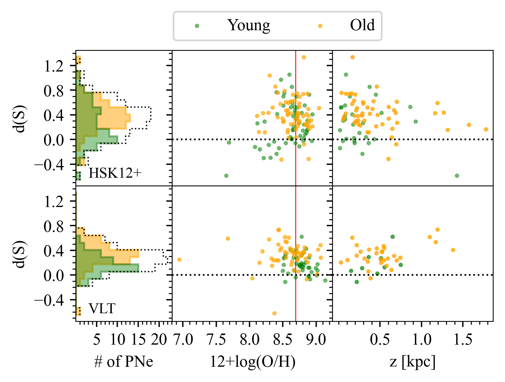
Figure 4: A combined figure for sulfur deficit $d$(S) on the vertical axis for the HSK12+ sample (top row) and VLT sample (bottom row) against i) histograms of $d$(S) values with a bin size of 0.11 dex, ii) 12+$\log$(O/H) and iii) absolute height above the Galactic plane ‘$|z|$’ in kpc. The Galactic disk and bulge PNe samples are color-coded to their basic age group from criteria outlined in Appendix C. Green indicates young and orange indicates old progenitor stars according to the adopted dating scheme. The grey dashed line in the left panel outlines the overall distribution. The middle panel red vertical line indicates solar oxygen abundance.

5.5 PNe dust chemistry

AGB stars produce different dust grains based on their C/O abundance ratio. Possible gas phase sulfur depletion due to dust or molecule formation was investigated in Henry et al. (2012). They concluded it is unlikely to explain the sulfur anomaly as no correlation between $d$(S) and C/O ratios was seen. The formation of key sulfur-bearing compounds, MgS and FeS, depends on a C-rich (C/O $>1$) environment in AGB stars (e.g. Nuth et al., 1985; Lodders & Fegley Jr, 1995). However, to classify PNe as C-rich or O-rich (C/O $<1$), observing the dust features in their infrared spectra is a more reliable way than measuring the C/O abundance ratios from optical emission lines. The latter could be affected by uncertainties and depletion of carbon or oxygen into dust grains (Delgado-Inglada et al., 2015).

PNe dust features from Spitzer (García-Hernández & Górny, 2014) show that 33% of Galactic disk PNe and 8% of bulge PNe have C-rich dust features. Such C-rich PNe generally have sub-solar O/H and a larger sulfur deficit (median $d$(S)$=$0.51 dex) while those with O-rich or C-rich and O-rich dust features (dual chemistry) scatter above and below the BCG data, with median $d$(S) values of 0.34 and 0.07 dex (see their Fig. 8).

This work suggests missing gas-phase sulfur in C-rich PNe could be due to efficient dust formation, while reduced sulfur deficit in O-rich objects may be due to sulfur depletion into molecules (e.g. SO, SO2, H2S, and CS Omont et al., 1993; Bujarrabal et al., 1994) in C-rich and O-rich environments. Furthermore, Delgado-Inglada et al. (2015) found that C-rich PNe with sub-solar O/H were enriched in oxygen by $\sim 0.3$ dex. Hence, the sulfur deficit in C-rich nebulae may be due to both dust and/or molecule depletion and oxygen enrichment, while gas-phase sulfur depletion into molecules leads to a smaller sulfur deficit in oxygen rich PNe.

AGB star evolution can lead to transformation of low to intermediate mass stars (1.5-4$M_{\odot}$) from O-rich to C-rich stars through the efficient third dredge-up process (Karakas & Lattanzio, 2014). However, low-mass stars ($\leq 1.5$$M_{\odot}$) and more massive stars ($>$ 3-4$M_{\odot}$) which are classified as young PNe in this study, are expected to remain O-rich throughout their evolution.

6 Summary

Based on our robust abundances for a significant sample of Galactic bulge PNe, we report important new insights into the PNe sulfur anomaly while reducing its significance. We rule out some previous suggestions of where it might originate and validate others that contribute to its reduced form. We reveal that it is the young and more massive progenitors of the current PNe population and their associated dust chemistry that show low or absent sulfur deficit. Our key findings are:

* we show lockstep behaviour for sulfur versus both oxygen and argon abundances for the first time, emphasising the role high-quality data plays

* adopting the DMS14 ICF scheme reduces the sulfur anomaly as our machine learning approach shows

* based on mid-infrared data for a small, overlapping PNe sample, we find the sulfur anomaly is unlikely due to underestimation of higher sulfur ionization stages in the photoionization models and their derived ICFs

* the impact of different extinction laws on the sulfur anomaly is insignificant

* the sulfur deficit is not due to weak sulfur line fluxes in the optical range. While IFU observations show sampling whole PNe is important for an overall sulfur deficit determination it is also reduced for some PNe

* correlations of lower sulfur deficit with Galactic height above/below the mid-plane and their close relation to PNe progenitor mass and chemistry are shown

* the sulfur deficit is almost absent for PNe from higher mass, younger progenitors and those with oxygen or dual dust chemistry related to progenitor mass. Larger deficits for intermediate progenitor mass PNe that are carbon rich are seen, the solution is likely there

Appendix A Comparison of Ne/H and Ar/H versus O/H relationships using optical and mid- infrared observation

We present additional figures that give a comparison of Ne/H and Ar/H with O/H and with Ne/H and Ar/H derived from both the optical VLT data from Paper III and the mid-infrared observations presented in PBS15.

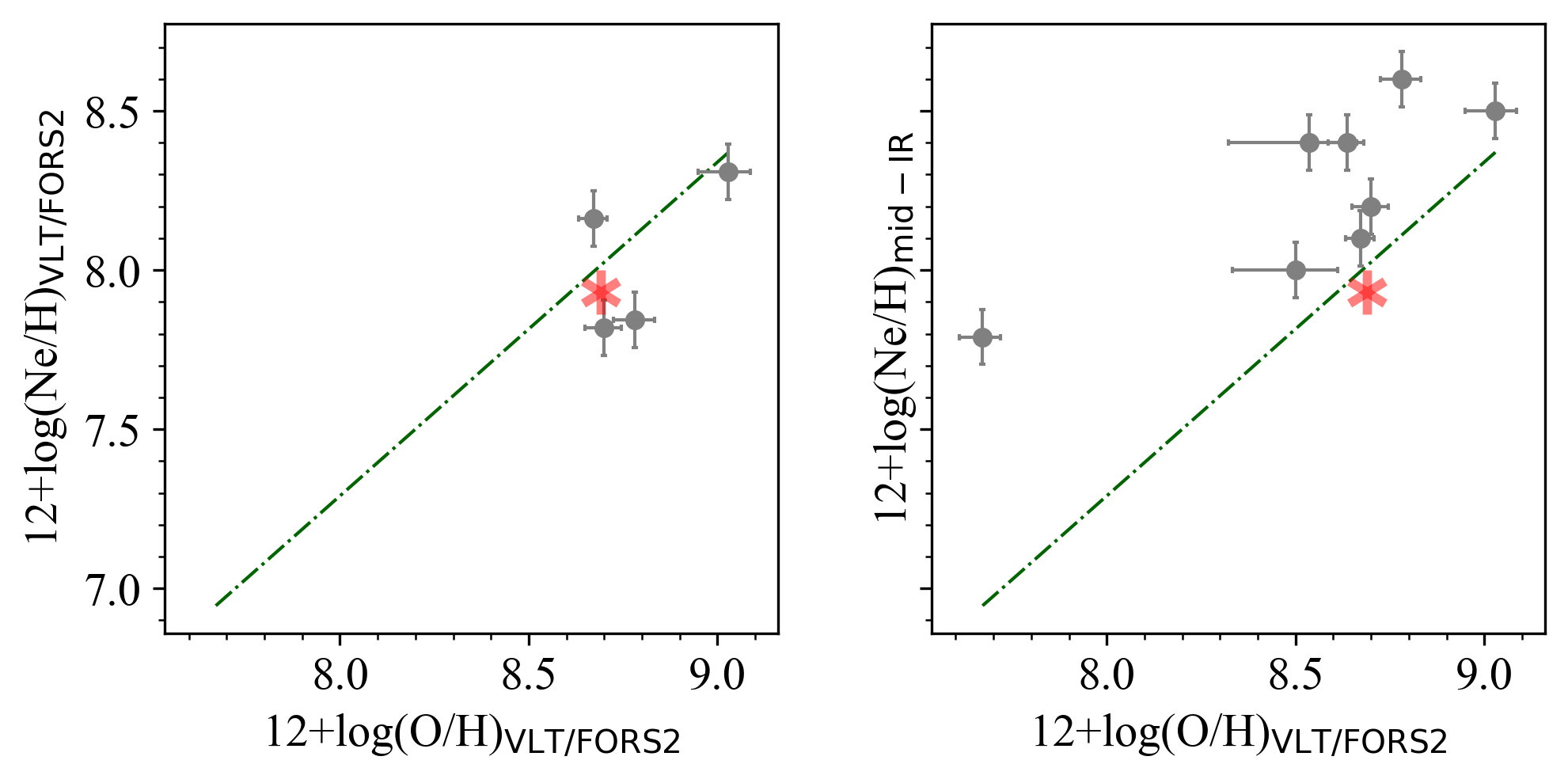
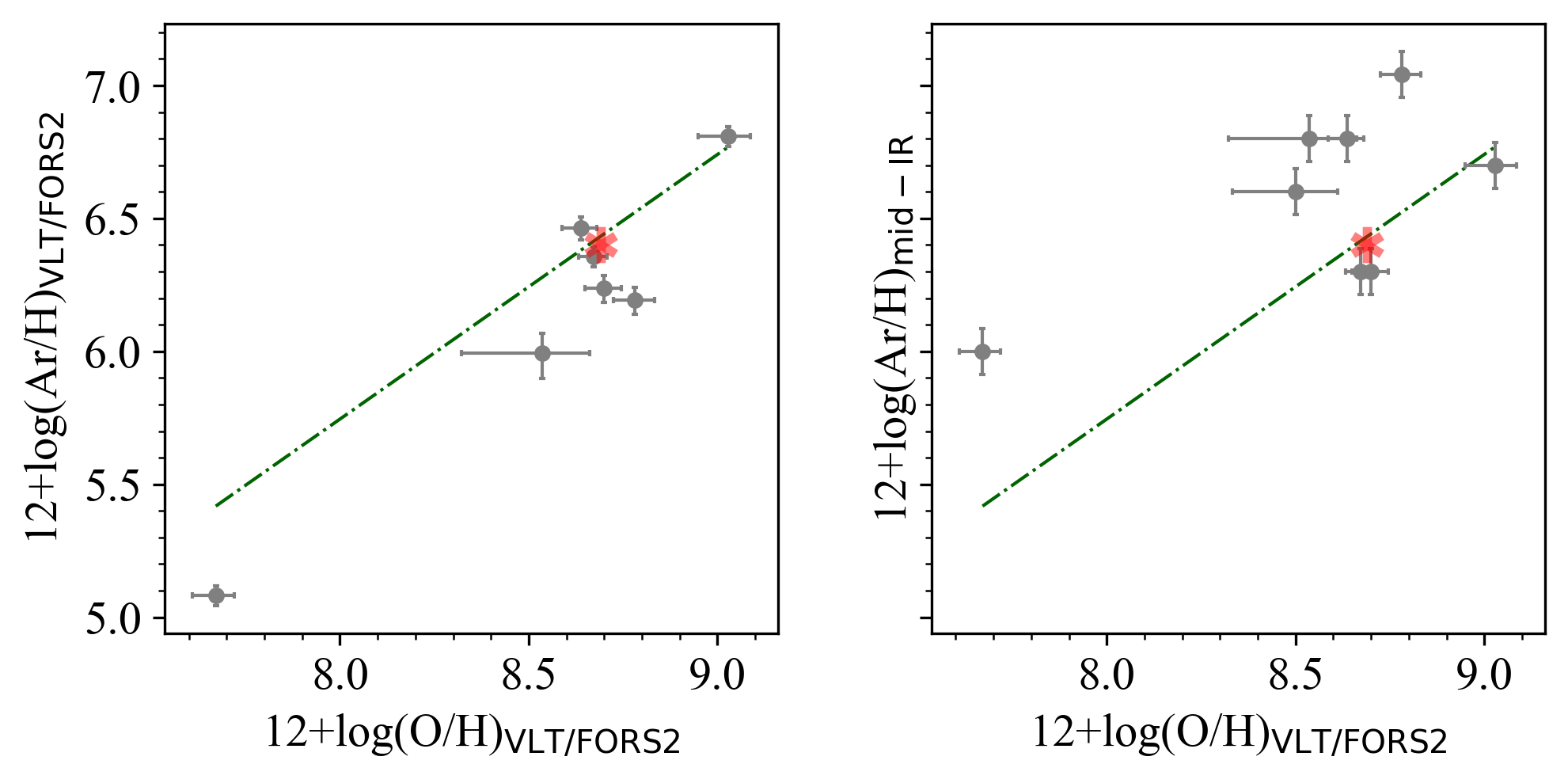
Figure A1: Comparison of Ne/H and Ar/H versus O/H relationships using optical VLT observations and mid-infrared observations in PBS15, with symbols defined in Fig. 3.

Appendix B Selection of hyperparameters and performance evaluation for the random forest regressor

The RF regressors, used to predict either the ionic fraction or the icf(S), all attained an $R^{2}$ of 0.99, indicating a reliable regression. For ICF values for sulfur, icf(S), used when S²⁺ is observed, i.e. icf(S)$=$S/(S⁺+S²⁺), the fractional differences between the predicted and actual test sample values are generally $<5\%$. Only 0.9% of cases exceed 15% fractional differences (primarily for icf(S) values from 2.5 to 15). The median fractional difference is near zero (0.0002). This suggests no systematic bias between the predicted and true icf(S) values of the test set. For the icf(S) values used when only S⁺ is observed, icf(S)$=$S/S⁺, predicted values exhibit slightly larger deviations from test sample actual values. Nonetheless, the fractional difference is $<15\%$ for $\sim$92% of cases, with a median fractional difference of 0.005. This indicates no significant systematic differences between the predicted and true icf(S) values of the test set.

To enhance the performance of the RF regressor, which was used for predicting either icf(S) or unobserved ionic fractions, we compared different sets of hyperparameters using the k-fold cross-validation (CV) on the validation set. The hyperparameters tuned for RF include the number of trees, (n_estimators), the maximum depth of each tree, (max_depth), the number of features allowed to make the best split while building the tree, (max_features), minimum number of samples to split an internal node (min_samples_split), minimum number of samples to form a leaf node (min_samples_leaf) and whether bootstrap samples are used when building trees (bootstrap). The default values were used for the remaining hyperparameters.

B.1 RF regressor for icf(S)

For icf(S), the RF model generates highly accurate predictions for both S/(S²⁺+S⁺) and S/S⁺, with $R^{2}$ values exceeds 0.99. We presents the fractional uncertainties in predicted icf(S) with respect to the true values of the test set as a function of true icf(S) values on a log scale in Fig.B1 for icf(S)$=$S/(S²⁺+S⁺) (top panel) and icf(S)$=$S/S⁺ (bottom panel). Both RF regressors exhibit no systematical discrepancies from the actual values, with most of the predicted values having a fractional uncertainty less than 5% and 10%, respectively. Although, the upper panel of Fig.B1 reveals slightly higher predicted values than the actual values for intermediate S/(S²⁺ + S⁺) values ($\sim 1.26$ to 3.16), the median fractional uncertainty within this range is 0.01 dex. Thus, no systematical bias in predicted values presents for this range.

2*Parameter	2*Grid	Optimal parameter
		S/(S2++S+)	S/S+
n_estimators	[100, 600]	500	100
min_samples_split	[2, 7]	3	3
min_samples_leaf	[1, 10]	2	1
max_depth	[5, 50]	13	50
max_features	[sqrt, auto]	sqrt	sqrt
bootstrap	[True, False]	False	True

Table B1: Hyperparameter adjustments for icf(S) RF regressors.

Each model’s performance was evaluated with a 5-fold CV and quantified by the mean squared error (MSE) between the predictions and true values of the validation set. We used RandomizedSearchCV from scikit-learn to randomly select a subset of 50 among all combinations of $\alpha$ values. The best parameter selections are presented in Table B1. The optimal set of $\alpha$ values, which minimised the MSE, was chosen to train the final model. This model was then trained on the training set and applied to the test set.

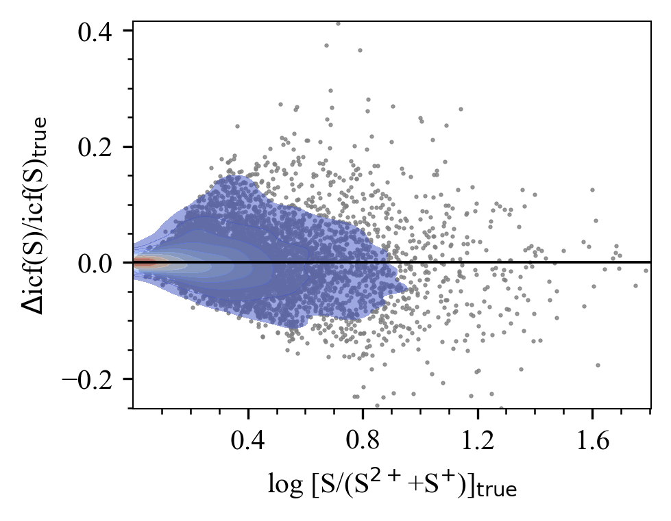
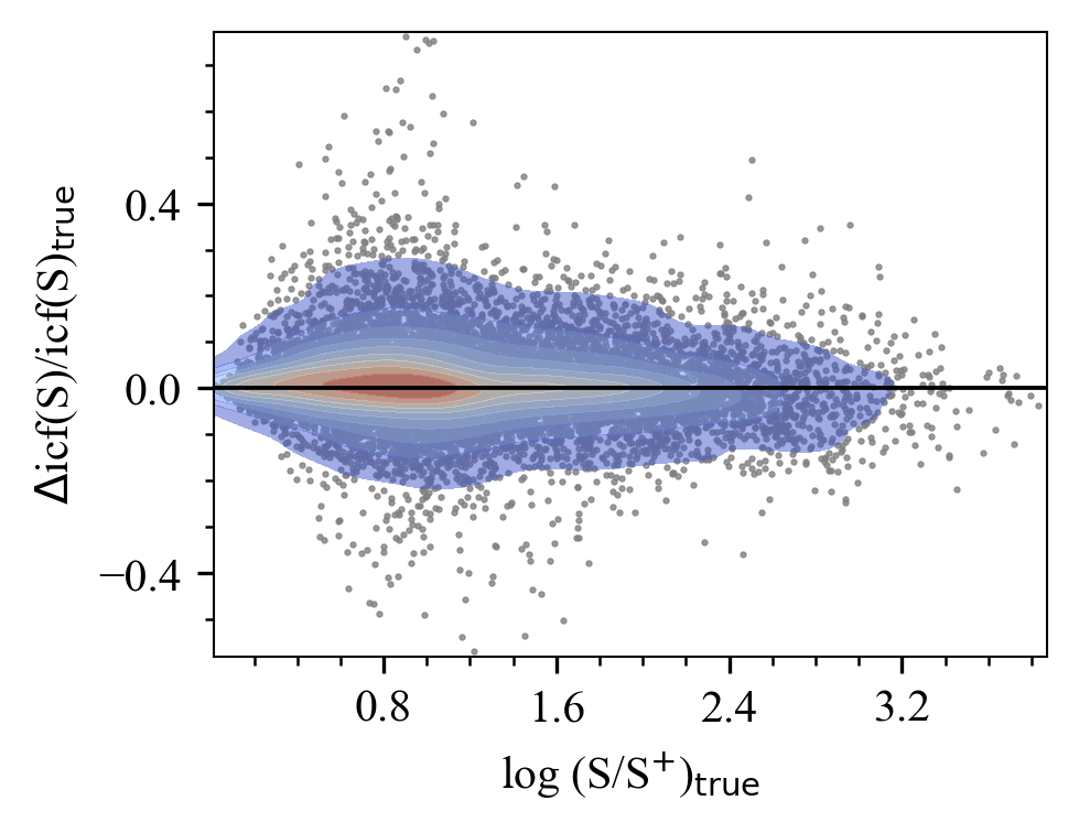
Figure B1: Fractional uncertainty in predicted icf(S) from the RF regressor as a function of log-scale true icf(S) for the test set. The contours illustrate the number density based on kernel density estimation. The black solid line denotes zero fractional uncertainty, with a high concentration of data points along this line indicating no systematic discrepancy between the predicted icf(S) from the RF regressor and the true values from the test set.

B.2 RF regressor for Ar and Cl ionic fractions

We used two separated RF regressors to predict the unobserved ionic fraction, Ar³⁺/Ar²⁺, Cl³⁺/Cl²⁺, which are then used as input features to predict icf(S). Similarly, the hyperparameters were tuned through a 5-fold CV. We used GridSearchCV from scikit-learn to test all possible combinations of $\alpha$ values. The parameter grids and best parameter selections are presented in Table.B2. Using He²⁺/He⁺ and O²⁺/O⁺ as the input features, the RF models to predict Ar³⁺/Ar²⁺ and Cl³⁺/Cl²⁺ achieved $R^{2+}$ values of 0.99.

2*Parameter	2*Grid	Optimal parameter
		Ar3+/Ar2+	Cl3+/Cl2+
n_estimators	[500, 2E3, 2E3]	2E3	1E3
min_samples_split	[2, 4, 6]	2	6
min_samples_leaf	[1, 5]	1	1
max_depth	[50, 75, 100]	75	100
max_features	[sqrt, auto]	auto	auto
bootstrap	[True, False]	True	True

Table B2: Hyperparameter adjustments for Ar³⁺/Ar²⁺ and Cl³⁺/Cl²⁺ RF regressors.

The fractional uncertainties in Ar³⁺/Ar²⁺ and Cl³⁺/Cl²⁺ as a function of the ionic fractions on a log scale is given in Fig.B2. The predicted values show larger deviation when Ar²⁺ or Cl²⁺ is the dominant ionization stage of Ar or Cl. Still, the predicted values agree with the true values of the test set within 50% for 89% and 90% of the cases.

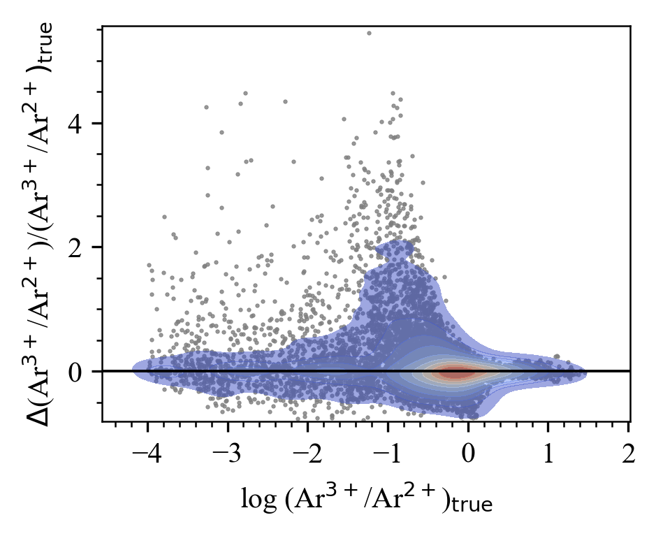
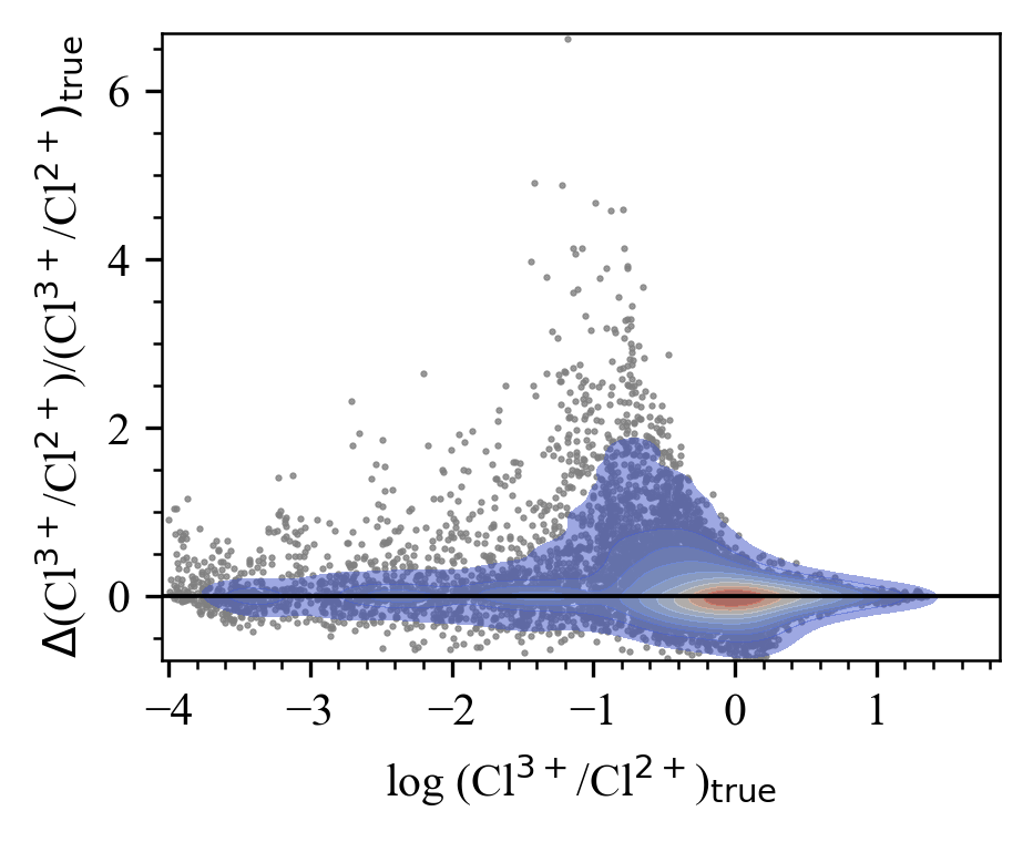
Figure B2: Fractional uncertainty in predicted Ar³⁺/Ar²⁺ (left) and Cl³⁺/Cl²⁺ (right) from the RF regressor as a function of log-scale true ionic fractions of the test set. The plots were constructed in the same manner as Fig.B1.

Appendix C Classifying Planetary Nebulae into basic Young and Old Groups

Based on previous studies on PNe abundances, Peimbert (1978) divided PNe into four distinct types, each with unique general properties. Type I PNe are those enriched in He and N abundances (He/H$>0.125$ and $\log$(N/O)$>-0.3$, as defined in Peimbert & Torres-Peimbert, 1983), and they typically exhibit bipolar morphologies, high central star temperatures, and lower mean scale-heights above the Galactic plane (Corradi & Schwarz, 1995; Peimbert & Torres-Peimbert, 1983). These properties are consistent with more massive progenitors compared to other PNe nuclei, as younger and more massive stars are likely to form in a more enriched ISM and undergo more efficient ‘dredge-up’ processes (Phillips, 2005), leading to higher He and N abundances. The progenitor masses of Type I PNe are suggested to be greater than $2.4M_{\odot}$ (Peimbert & Serrano, 1980; Calvet & Peimbert, 1983), with small variations in the literature, corresponding to an stellar age of about 1 Gyr.

Using AGB evolutionary models that incorporate dust formation in circumstellar envelopes, Ventura et al. (2016) investigated the relationship between progenitor masses and chemical composition of the resulting PNe. They found that carbon stars produce C-rich PNe by ejecting their shells, while stars undergoing hot-bottom burning, a phase during which most of their C is converted into N, do not go through the carbon star phase and instead eject a N-rich shell. These findings were used to classify PNe into young and old populations according to their C/H and N/H ratios in Stanghellini & Haywood (2018), hereafter referred to as SH18. A similar classification scheme using O/H instead of C/H was also derived in SH18 as follows: for the old PNe population with a stellar age greater than 7.5 Gyr, $12+\log$(N/H)$<0.8\times[12+\log$(O/H)$]+1.4$; and for the young PNe population with the central stars younger than 1 Gyr, $12+\log$(N/H)$>0.6\times[12+\log$(O/H)]$+3.3$.

We consider both PN dating methods as equally reliable. We select a group of young PNe where the two schemes yield non-contradictory results, meaning objects are either classified as young based on the SH18 criteria and are Type I, or are Type I PNe without an age group determined by the SH18 scheme. Similarly, we choose a group of old PNe that are classified as old using the SH18 criteria and are not Type I objects. Despite the large uncertainties, which may exceed 3-4 Gyr due to the abundance determination and the dating methods themselves, the young PNe group’s progenitor ages are estimated to be less than 1 Gyr, while the old PNe population is expected to descend from those older than 7.5 Gyr. Despite this crude age demarcation, a clear effect in the size and distribution of the sulfur anomaly is shown in Fig. 4 in the main body of the text, between the young and old PNe populations.

It is important to note that this age classification relies on the single-star assumption for CSPNe. The presence of companion stars, particularly in close-binary systems, can affect their evolutionary pathways and introduce uncertainty in age estimation (see e.g. Soderblom, 2010; Stanway & Eldridge, 2018).

References

- Ali et al. (2016) Ali, A., Dopita, M., Basurah, H., et al. 2016, Monthly Notices of the Royal Astronomical Society, 462, 1393
- Bandyopadhyay et al. (2021) Bandyopadhyay, R., Das, R., & Mondal, S. 2021, Monthly Notices of the Royal Astronomical Society, 504, 816
- Breiman (2001) Breiman, L. 2001, Machine learning, 45, 5
- Bujarrabal et al. (1994) Bujarrabal, V., Fuente, A., & Omont, A. 1994, Astronomy and Astrophysics, Vol. 285, p. 247-271 (1994), 285, 247
- Calvet & Peimbert (1983) Calvet, N., & Peimbert, M. 1983, Revista Mexicana de Astronomia y Astrofisica, 5, 319
- Cardelli et al. (1989) Cardelli, J. A., Clayton, G. C., & Mathis, J. S. 1989, Astrophysical Journal, Part 1 (ISSN 0004-637X), vol. 345, Oct. 1, 1989, p. 245-256., 345, 245
- Cavichia et al. (2010) Cavichia, O., Costa, R., & Maciel, W. 2010, Revista mexicana de astronomía y astrofísica, 46, 159
- Chornay & Walton (2021) Chornay, N., & Walton, N. 2021, Astronomy & Astrophysics, 656, A110
- Corradi & Schwarz (1995) Corradi, R. L., & Schwarz, H. E. 1995, Astronomy and Astrophysics, Vol. 293, p. 871-888 (1995), 293, 871
- Delgado-Inglada et al. (2014) Delgado-Inglada, G., Morisset, C., & Stasińska, G. 2014, MNRAS, 440, 536, doi: 10.1093/mnras/stu341
- Delgado-Inglada et al. (2014) Delgado-Inglada, G., Morisset, C., & Stasińska, G. 2014, Monthly Notices of the Royal Astronomical Society, 440, 536
- Delgado-Inglada et al. (2015) Delgado-Inglada, G., Rodríguez, M., Peimbert, M., Stasińska, G., & Morisset, C. 2015, Monthly Notices of the Royal Astronomical Society, 449, 1797
- Dors Jr et al. (2013) Dors Jr, O. L., Hägele, G. F., Cardaci, M. V., et al. 2013, Monthly Notices of the Royal Astronomical Society, 432, 2512
- Ferland et al. (2017) Ferland, G., Chatzikos, M., Guzmán, F., et al. 2017, Revista mexicana de astronomía y astrofísica, 53
- Fitzpatrick (1999) Fitzpatrick, E. L. 1999, Publications of the Astronomical Society of the Pacific, 111, 63
- Freeman et al. (2013) Freeman, K., Ness, M., Wylie-de-Boer, E., et al. 2013, MNRAS, 428, 3660, doi: 10.1093/mnras/sts305
- García-Hernández & Górny (2014) García-Hernández, D., & Górny, S. 2014, Astronomy & Astrophysics, 567, A12
- García-Hernández & Górny (2014) García-Hernández, D. A., & Górny, S. K. 2014, A&A, 567, A12, doi: 10.1051/0004-6361/201423620
- García-Rojas et al. (2022) García-Rojas, J., Morisset, C., Jones, D., et al. 2022, Monthly Notices of the Royal Astronomical Society, 510, 5444
- González-Santamaría et al. (2021) González-Santamaría, I., Manteiga, M., Manchado, A., et al. 2021, Astronomy & Astrophysics, 656, A51
- Gould et al. (2001) Gould, A., Stutz, A., & Frogel, J. A. 2001, The Astrophysical Journal, 547, 590
- Henry et al. (2010) Henry, R., Kwitter, K. B., Jaskot, A. E., et al. 2010, The Astrophysical Journal, 724, 748
- Henry et al. (2004) Henry, R. B., Kwitter, K., & Balick, B. 2004, The Astronomical Journal, 127, 2284
- Henry et al. (2012) Henry, R. B., Speck, A., Karakas, A. I., Ferland, G. J., & Maguire, M. 2012, The Astrophysical Journal, 749, 61
- Howarth (1983) Howarth, I. D. 1983, Monthly Notices of the Royal Astronomical Society, 203, 301
- Izotov & Thuan (1999) Izotov, Y. I., & Thuan, T. X. 1999, The Astrophysical Journal, 511, 639
- Karakas & Lattanzio (2014) Karakas, A. I., & Lattanzio, J. C. 2014, Publications of the Astronomical Society of Australia, 31, e030
- Kennicutt Jr et al. (2003) Kennicutt Jr, R. C., Bresolin, F., & Garnett, D. R. 2003, The Astrophysical Journal, 591, 801
- Kingsburgh & Barlow (1994) Kingsburgh, R. L., & Barlow, M. 1994, Monthly Notices of the Royal Astronomical Society, 271, 257
- Kwitter & Henry (2001) Kwitter, K., & Henry, R. 2001, The Astrophysical Journal, 562, 804
- Li & Zhao (2017) Li, C., & Zhao, G. 2017, The Astrophysical Journal, 850, 25
- Lodders & Fegley Jr (1995) Lodders, K., & Fegley Jr, B. 1995, Meteoritics, 30, 661
- Mathis (1985) Mathis, J. S. 1985, ApJ, 291, 247, doi: 10.1086/163063
- Milingo et al. (2010) Milingo, J., Kwitter, K., Henry, R., & Souza, S. 2010, The Astrophysical Journal, 711, 619
- Morisset et al. (2015) Morisset, C., Delgado-Inglada, G., & Flores-Fajardo, N. 2015, Revista mexicana de astronomía y astrofísica, 51, 101
- Nuth et al. (1985) Nuth, J. A., Moseley, S. H., Silverberg, R. F., Goebel, J. H., & Moore, W. J. 1985, Astrophysical Journal, Part 2-Letters to the Editor (ISSN 0004-637X), vol. 290, March 1, 1985, p. L41-L43., 290, L41
- Omont et al. (1993) Omont, A., Lucas, R., Morris, M., & Guilloteau, S. 1993, Astronomy and Astrophysics (ISSN 0004-6361), vol. 267, no. 2, p. 490-514., 267, 490
- Otsuka et al. (2017) Otsuka, M., Ueta, T., Van Hoof, P. A., et al. 2017, The Astrophysical Journal Supplement Series, 231, 22
- Parker et al. (2022) Parker, Q. A., Xiang, Z., & Ritter, A. 2022, Galaxies, 10, 32
- Pedregosa et al. (2011) Pedregosa, F., Varoquaux, G., Gramfort, A., et al. 2011, the Journal of machine Learning research, 12, 2825
- Peimbert (1978) Peimbert, M. 1978, in Symposium-International Astronomical Union, Vol. 76, Cambridge University Press, 215–224
- Peimbert & Serrano (1980) Peimbert, M., & Serrano, A. 1980, Revista Mexicana de Astronomia y Astrofisica, vol. 5, Apr. 1980, p. 9-18., 5, 9
- Peimbert & Torres-Peimbert (1983) Peimbert, M., & Torres-Peimbert, S. 1983, in Symposium-International Astronomical Union, Vol. 103, Cambridge University Press, 233–242
- Phillips (2005) Phillips, J. 2005, Monthly Notices of the Royal Astronomical Society, 361, 283
- Pottasch & Bernard-Salas (2015) Pottasch, S., & Bernard-Salas, J. 2015, Astronomy & Astrophysics, 583, A71
- Reichel et al. (2022) Reichel, M., Kimeswenger, S., van Hoof, P. A., et al. 2022, The Astrophysical Journal, 939, 103
- Robitaille et al. (2013) Robitaille, T. P., Tollerud, E. J., Greenfield, P., et al. 2013, Astronomy & Astrophysics, 558, A33
- Sabin et al. (2022) Sabin, L., Gómez-Llanos, V., Morisset, C., et al. 2022, MNRAS, 511, 1, doi: 10.1093/mnras/stab3649
- Shingles & Karakas (2013) Shingles, L. J., & Karakas, A. I. 2013, MNRAS, 431, 2861, doi: 10.1093/mnras/stt386
- Smirnov (1939) Smirnov, N. V. 1939, Bull. Math. Univ. Moscou, 2, 3
- Soderblom (2010) Soderblom, D. R. 2010, Annual Review of Astronomy and Astrophysics, 48, 581
- Stanghellini & Haywood (2018) Stanghellini, L., & Haywood, M. 2018, The Astrophysical Journal, 862, 45
- Stanway & Eldridge (2018) Stanway, E. R., & Eldridge, J. 2018, Monthly Notices of the Royal Astronomical Society, 479, 75
- Tan et al. (2023) Tan, S., Parker, Q. A., Zijlstra, A., & Ritter, A. 2023, Monthly Notices of the Royal Astronomical Society, 519, 1049
- Tan et al. (2024) Tan, S., Parker, Q. A., Zijlstra, A. A., & Rees, B. 2024, MNRAS, 527, 6363, doi: 10.1093/mnras/stad3496
- Udalski (2003) Udalski, A. 2003, The Astrophysical Journal, 590, 284
- Ventura et al. (2016) Ventura, P., Stanghellini, L., Di Criscienzo, M., García-Hernández, D., & Dell’Agli, F. 2016, Monthly Notices of the Royal Astronomical Society, 460, 3940