Five Starter Problems: Solving Quadratic Unconstrained Binary Optimization Models on Quantum Computers

Abstract

Several articles and books adequately cover quantum computing concepts, such as gate/circuit model (and Quantum Approximate Optimization Algorithm, QAOA), Adiabatic Quantum Computing (AQC), and Quantum Annealing (QA). However, they typically stop short of accessing quantum hardware and solve numerical problem instances. This tutorial offers a quick hands-on introduction to solving Quadratic Unconstrained Binary Optimization (QUBO) problems on currently available quantum computers. We cover both IBM and D-Wave machines: IBM utilizes a gate/circuit architecture, and D-Wave is a quantum annealer. We provide examples of three canonical problems (Number Partitioning, Max-Cut, Minimum Vertex Cover), and two models from practical applications (from cancer genomics and a hedge fund portfolio manager, respectively). An associated GitHub repository provides the codes in five companion notebooks. Catering to undergraduate and graduate students in computationally intensive disciplines, this article also aims to reach working industry professionals seeking to explore the potential of near-term quantum applications.

1 Introduction

Quantum Computing is one of the most promising new technologies of the 21st century. Due to the nascency of the hardware, however, many of these envisioned speedups remain largely theoretical. Despite the limitations of available quantum hardware, there is significant interest in exploring them. While several articles and books (see [20] for example) adequately cover the principles of quantum computing, they typically stop short of providing a road map to access quantum hardware and numerically solve problems of interest. This tutorial is aimed at providing quick access to both IBM and D-Wave machines, thereby covering two types of quantum algorithms, one based on gate/circuit model [23] and the other on quantum annealing [18], with Notebooks containing associated software. We hope that our tutorial can serve as a companion to the available books and articles.

We first briefly introduce Quadratic Unconstrained Optimization (QUBO) and Ising models. We then show how they capture three canonical combinatorial optimization problems: Number Partitioning [19], Max-Cut [7], and Minimum Vertex Cover [6]. We next model two practical problems: de novo discovery of driver genes (cancer genomics) [1] and Order Partitioning (for A/B testing at a hedge fund portfolio manager). We then provide step-by-step instructions to solve the QUBOs across two frameworks: gate/circuit model (IBM hardware [22]) and quantum annealing (D-Wave hardware [5]).

2 Quadratic Unconstrained Binary Optimization and Ising models: The Bare Minimum

Quadratic Unconstrained Binary Optimization (QUBO) models can be used to represent a variety of problems [4] [12]. The general matrix form of a QUBO is:

$$min_{\mathbf{x}\in\{0,1\}^{n}}[\mathbf{x}^{T}\mathbf{Q}\mathbf{x}+c].$$ (1)

Here $\mathbf{x}$ represents a binary solution vector of size $n$, $\mathbf{Q}$ is an upper triangular matrix, and $c$ is an arbitrary constant. (Note that $c$ makes no difference to the optimal solution.) After multiplying out the matrix form, the resulting equation is a quadratic unconstrained binary optimization model, QUBO:

$$min_{x\in\{0,1\}^{n}}[\sum_{ij}Q_{ij}x_{i}x_{j}+\sum_{i}Q_{ii}x^{2}_{i}+c].$$ (2)

Since $\mathbf{x}$ is a binary vector, $x^{2}_{i}=x_{i}$, we obtain (a triangular form):

$$min_{x\in\{0,1\}^{n}}[\sum_{i<j}Q_{ij}x_{i}x_{j}+\sum_{i}Q_{ii}x_{i}+c].$$ (3)

QUBO models are a natural gateway to quantum computing due to their link with computer science and their mathematical equivalence to the Ising model [17] in physics. The generic form of an Ising model is:

$$H(\sigma)=-\sum_{ij}J_{ij}\sigma_{i}\sigma_{j}-\sum_{i}h_{i}\sigma_{i}$$ (4)

where $H$ is the hamiltonian or energy of the system, $\sigma_{i}$ being the spin $\{-1,+1\}$ at site $i$, $J_{ij}$ is the interaction between sites, and $h_{i}$ is the external field applied at each site. QUBO can be mapped to an Ising model using the transformation $\sigma_{i}=2x_{i}-1$ and conversely, the conversion from Ising to QUBO is $x_{i}=\frac{\sigma_{i}+1}{2}$.

3 Three Canonical Problems

3.1 Number Partitioning

The Number Partitioning problem goes as follows: Given a set $S$ of positive integer values $\{s_{1},s_{2},s_{3}...s_{n}\}$, partition $S$ into two sets $A$ and $S/A$ such that:

$$d=|\sum_{s_{i}\in A}s_{i}-\sum_{s_{j}\in S/A}s_{j}|$$

is minimized. If $d=0$, there is a perfect partition that needs to be found; otherwise $d$ should be made as small as possible.

This objective function can be expressed as a QUBO by using the binary variable: $x_{i}=1$ indicates that $s_{i}$ belongs to $A$ and $x_{i}=0$ means $s_{i}$ in $S/A$. The sum of elements in $A$ is $\sum_{i=1}^{n}s_{i}x_{i}$ and the sum of elements in $S/A$ is $c-\sum_{i=1}^{n}s_{i}x_{i}$, where $c$ is the sum of elements of $S$, a constant. Thus, the difference in the sums is:

$$d=c-2\sum_{i=1}^{n}s_{i}x_{i}.$$

This difference is minimized by minimizing the QUBO:

$$d^{2}=(c-2\sum_{i=1}^{n}s_{i}x_{i})^{2}=c^{2}+4\mathbf{x}^{T}\mathbf{Q}\mathbf{x}$$

with $q_{ij}$ entry in $\mathbf{Q}$ being:

$$q_{ij}=\begin{cases}s_{i}(s_{i}-c)&\text{if }i=j\\ s_{i}s_{j}&\text{if }i\neq j\end{cases}$$

3.2 Max Cut

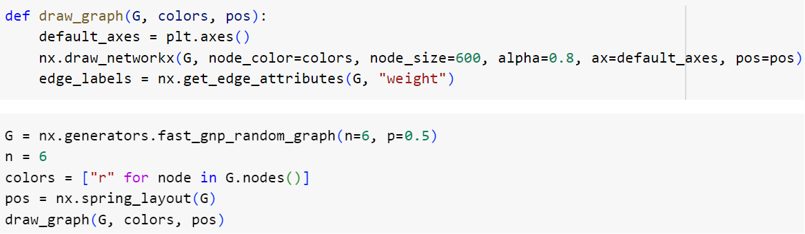
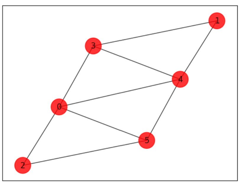
Figure 9: Code for Max-Cut Problem Instance

Figure 10: Max-Cut Graph

The Max-Cut Problem goes as follows: Given an undirected graph, $G$ with vertex set $V$ and edge set $E$, partition $V$ in sets $A$ and $V/A$ such that the number of edges connecting nodes between these two sets is maximized. See Figure 10 for a graph with six nodes labeled $0,1,2,3,4,5$ and eight edges.

Similar to Number Partitioning, the QUBO can be constructed by setting $x_{i}=1$ if vertex $i$ is in $A$ and letting $x_{i}=0$ if vertex $i$ is in $V/A$. The expression $x_{i}+x_{j}-2x_{i}x_{j}$ identifies whether edge $(i,j)\in E$ is in the cut: $x_{i}+x_{j}-2x_{i}x_{j}$ is $1$ if and only if exactly one of $x_{i}$ or $x_{j}$ is $1$ (and the other is $0$). The objective function is:

$$\max[\sum_{(i,j)\in E}x_{i}+x_{j}-2x_{i}x_{j}].$$

Since QUBOs are typically framed as minimization problems, the Max-Cut QUBO is:

$$\min[\sum_{(i,j)\in E}2x_{i}x_{j}-(x_{i}+x_{j})].$$

3.3 Minimum Vertex Cover

As the name implies, the Minimum Vertex Cover problem seeks to find the minimum vertex cover of an undirected graph $G$ with vertex set $V$ and edge set $E$. A vertex cover is the subset of vertices such that each edge $(i,j)\in E$ shares an endpoint with at least one vertex in the subset.

The Minimum Vertex Cover problem has two features:

1. the number of vertices in the vertex cover must be minimized, and

2. the edges must be covered by the vertices. (All edges must share at least one vertex from the subset of vertices.)

If the inclusion of each vertex in the vertex cover is denoted with a binary value ($1$ if it is in the cover, and $0$ if it is not), the minimal vertex constraint can be expressed as:

$$Q_{1}=\sum_{i\in V}x_{i}.$$ (5)

Similar to Max-Cut, the covering criteria is represented with the constraint ((for all $(i,j)\in E)$):

$$x_{i}+x_{j}\geq 1.$$ (6)

This can be represented with the use of a penalty $P$:

$$Q_{2}=P(\sum_{(i,j)\in E}(1-x_{i}-x_{j}+x_{i}x_{j})).$$ (7)

Thus, the QUBO for Minimum Vertex Cover is to minimize:

$$\sum_{i\in V}x_{i}+P(\sum_{(i,j)\in E}(1-x_{i}-x_{j}+x_{i}x_{j})).$$ (8)

The value $P$ determines how strictly the covering criteria must be enforced. A higher $P$ will ensure the vertex set covers the graph, at the expense of guaranteeing finding the minimal set. On the other hand, a lower $P$ will have fewer elements in the vertex set but the set may not cover the graph.

4 Two Practical Problems

4.1 Cancer Genomics

The first application is to identify altered cancer pathways from shared mutations and gene exclusivity. There are two key combinatorial criteria essential to identifying driver mutations:

• Coverage: We want to identify which genes are most prevalent among cancer patients. If a gene is shared between many cancer patients, it is more likely that the gene is a driver gene.

• Exclusivity: If there is already an identified cancer gene in the patient’s gene list, it is less likely for there to be another. This is not a hard rule and is sometimes violated.

Based on the above, we obtain the following two matrices:

• Degree Matrix $\mathbf{D}$: This diagonal matrix corresponds to the coverage criterion. Each $d_{ij}$ index where $i=j$ represents the number of patients that are affected by gene $i$. This attribute should be maximized.

• Adjacency Matrix $\mathbf{A}$: This adjacency matrix corresponds to the exclusivity criterion. Each $a_{ij}$ with $i\neq j$ represents the number of patients affected by gene $i$ and gene $j$. This attribute should be minimized.

Let us begin with attempting to find just one pathway. We define a solution pathway as $\mathbf{x}=\begin{bmatrix}x_{1}&x_{2}&x_{3}&...&x_{n}\end{bmatrix}^{T}$ where for all $i\in\{1,2,3,...n\}$, $x_{i}$ is a binary variable. If $x_{i}=0$, then gene $i$ is not present in the cancer pathway. If $x_{i}=1$, the gene is present in the cancer pathway. The exclusivity term is $\mathbf{x}^{T}\mathbf{A}\mathbf{x}$ and the coverage term is $\mathbf{x}^{T}\mathbf{D}\mathbf{x}$. Since we want the exclusivity term to be minimized and the coverage term to be maximized, the QUBO to identify cancer pathways from a set of genes is:

$$\mathbf{x}^{T}\mathbf{A}\mathbf{x}-\alpha\mathbf{x}^{T}\mathbf{D}\mathbf{x}$$

where $\alpha$ is a penalty coefficient. Since coverage is more important than exclusivity, we weigh it more, and so $\alpha\geq 1$. This QUBO can be written equivalently using the $a_{ij}$ and $d_{ij}$ values of $A$ and $D$ respectively as follows:

$$\sum_{i=1}^{n}\sum_{j=1}^{n}a_{ij}x_{i}x_{j}-\alpha\sum_{i=1}^{n}d_{i}x_{i}.$$

The previous QUBO can be extended to identify multiple cancer pathways in a single run. Let $\mathbf{X}=\begin{bmatrix}\mathbf{x_{1}}&\mathbf{x_{2}}&...&\mathbf{x_{k}}\end{bmatrix}^{T}$ where each $i\in\{1,2...k\}$, $\mathbf{x}_{i}$ represents a cancer pathway. Define $\mathbf{L}=\mathbf{A}+\mathbf{D}$, $k\times k$ identity matrix $I_{k}$, $n\times n$ identity matrix $I_{n}$, and $k\times k$ matrix of all $1$s, $J_{k}$. With the use of tensor products, $\mathbf{Q}_{main}=-I_{k}\otimes\mathbf{L}$ and $\mathbf{Q}_{orth}=(J_{k}-I_{k})\otimes I_{n}$, the final QUBO is:

$$\mathbf{X}^{T}(\mathbf{Q}_{main}+\alpha\mathbf{Q}_{orth})\mathbf{X}.$$

4.2 Order Partitioning

Order Partitioning is used for A/B testing of various strategies (being proposed by researchers at a Hedge Fund Manager) that are being evaluated for actual implementation. The Order Partitioning problem goes as follows. We are given a set of $n$ stocks each with an amount $q_{j}$ dollars totaling $T$ dollars ($\sum_{j=1}^{n}q_{j}=T$). There are $m$ risk factors with $i\in(1,2,3...m)$. Let $p_{ij}$ be the risk exposure to factor $i$ for stock $j$. The objective is to partition the stocks $j=1\ldots n$ into sets $A$ and $B$ such that:

1. $\sum_{j\in A}q_{j}=\sum_{i\in B}q_{j}=\frac{T}{2},$ and

2. for each factor $i=1\ldots m$: $\sum_{j\in A}p_{ij}=\sum_{j\in B}p_{ij}$.

If exact equality is not possible, then we want the absolute difference to be minimized:

1. $\min|\sum_{j\in A}q_{j}-\sum_{j\in B}q_{j}|$ and

2. for each factor $i=1\ldots m$: $\min|\sum_{j\in A}p_{ij}-\sum_{j\in B}p_{ij}|.$

When developing the QUBO for this problem, we must note that Objective $1$ is the same as the Number Partitioning problem, so we can reuse the QUBO derived earlier (replacing $s$ with $q$, and noting that $x_{j}$ is binary) and weight it with penalty coefficient $a$

$$Q_{1}=a(T-2\sum_{j=1}^{n}q_{j}x_{j})^{2}.$$ (9)

To partition each of the risk factors we can briefly consider Ising spins to minimize the magnitude of $\vec{h}$. Note that as mentioned earlier $p_{ij}$ is the risk factor $i$ for stock $j$ and $\sigma_{j}$ is its corresponding Ising Spin for each stock.

$$\vec{h}=\begin{bmatrix}p_{11}&p_{12}&p_{13}&\cdots&p_{1n}\\ p_{21}&p_{22}&p_{23}&\cdots&p_{2n}\\ p_{31}&p_{32}&p_{33}&\cdots&p_{3n}\\ \vdots&\vdots&\vdots&\vdots&\vdots&\\ p_{m1}&p_{m2}&p_{m3}&\cdots&p_{mn}\end{bmatrix}\begin{bmatrix}\sigma_{1}\\ \sigma_{2}\\ \sigma_{3}\\ \vdots\\ \sigma_{n}\end{bmatrix}$$ (10)

Taking the $2$-norm square of $\vec{h}$ we get:

$$\lVert\vec{h}\rVert^{2}=\sum_{i=1}^{m}(\sum_{j=1}^{n}p_{ij}\sigma_{j})^{2}.$$ (11)

Converting back to QUBO variables and weighting with $b$ we get:

$$Q_{2}=b\sum_{i=1}^{m}(\sum_{j=1}^{n}p_{ij}(2x_{j}-1))^{2}.$$ (12)

The complete QUBO for Order Partitioning is:

$$Q=a(T-2\sum_{j=1}^{n}q_{j}x_{j})^{2}+b\sum_{i=1}^{m}(\sum_{j=1}^{n}p_{ij}(2x_{j}-1))^{2}.$$ (13)

Note that $a$ and $b$ depend on how strictly each constraint is to be enforced.

5 Solving QUBOs on Quantum Computers

Three common algorithms are implemented: Quantum Approximate Optimization Algorithm (QAOA) [10], Quantum Annealing (QA) [9] and Simulated Annealing (SA) [15]. QAOA is implemented in three different ways on an IBM device: Vanilla QAOA (Notebook 1), OpenQAOA (Notebook 2) and via Qiskit (Notebook 3). Quantum Annealing (Notebook 4) and Simulated Annealing (Notebook 5) are implemented (on D-Wave) using the Annealing API from Ocean SDK. For brevity, in each of the five subsections, we detail only one of the five problems on one of the five algorithms, thereby covering all five problems on the five algorithms without repetition.

5.1 Vanilla QAOA

Regardless of the problem addressed, the vanilla QAOA implementation requires a Cost Hamiltonian, a Mixer Hamiltonian, and a QAOA Circuit. These were all implemented following the instructions provided by the Qiskit Textbook [3]. Here we focus on the Number Partitioning problem to illustrate the steps and the code.

5.1.1 Hamiltonians

The hyperparameters $\gamma,\beta$ are initialized to $0.5$. These parameters will be adjusted during the optimization phase for the QAOA circuit. For an arbitrary QUBO in the form of

$$\sum_{i,j=1}^{n}x_{i}Q_{ij}x_{j}+\sum_{i=1}^{n}c_{i}x_{i},$$

the Cost Hamiltonian was created by implementing $RZ$ gates across all angles $\theta_{1}$:

$$\theta_{1}=\frac{\gamma}{2}(\sum_{i=1}^{n}c_{i}+\sum_{i=1}^{n}Q_{ij}).$$

This layer of $RZ$ gates is followed by a layer of $ZZ$ gates applied on angles $\theta_{2}$:

$$\theta_{2}=\frac{1}{4}Q_{ij}\gamma.$$

The corresponding code and gates are shown below:

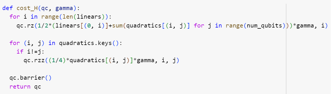
Figure 1: Code for Cost Hamiltonian

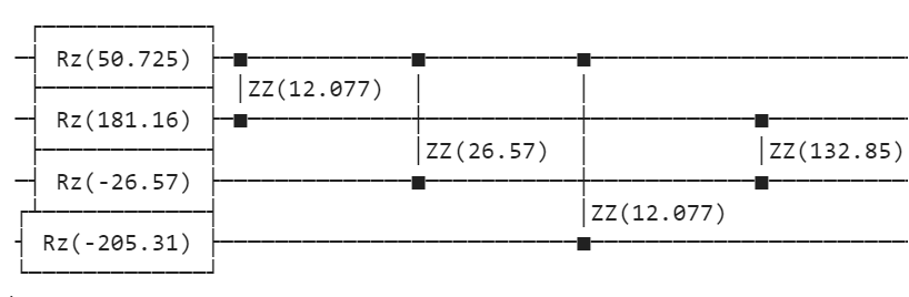
Figure 2: Cost Hamiltonian Gates

The Mixer Hamiltonian was created by applying $RX$ gates to angle $\theta_{3}$:

$$\theta_{3}=2\beta.$$

The code and gates are similarly shown below:

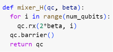
(a) Code for Mixer Hamiltonian

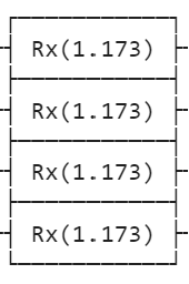
(b) Gates for Mixer Hamiltonian

Figure 3: Mixer Hamiltonian

5.1.2 QAOA Circuit

Once the Cost and Mixer Hamiltonians are defined, the final QAOA Circuit is then created by applying a layer of Hadamard Gates and then alternating between $p$ layers of Cost and Mixer Hamiltonians, before a final layer of measurements.

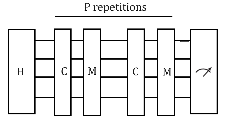
Figure 4: QAOA Circuit

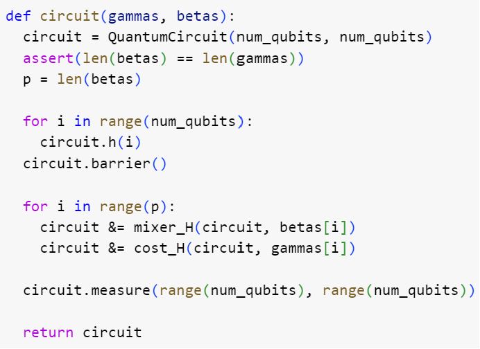
Figure 5: Code for Cost Hamiltonian

Once the generic framework is set up, the Number Partitioning QUBO quadratic and linear coefficients are substituted to replace the generic Cost and Mixer Hamiltonians implementations. The initial model is created using DOcplex [8], then converted into a QUBO, and then partitioned into quadratic and linear terms to implement each gate. The test example has $\{1,5,5,11\}$ as the set to be partitioned.

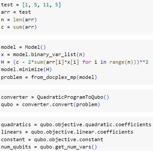
Figure 6: Creating the QUBO model

Once the circuit is created, its output is then optimized by adjusting the $\gamma,\beta$ using a classical optimizer. In order to optimize, we define an objective function and expectation function for the outputs of the circuit. The objective function measures the quality of QAOA output solutions while the expectation function averages these solutions over $1000$ shots. The optimizer then adjusts the solutions to minimize the expected objective value.

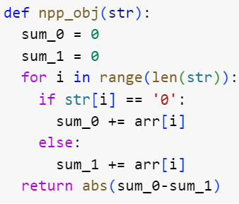
Figure 7: Number Partitioning objective function

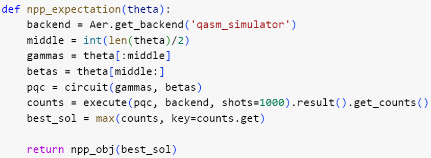
Figure 8: Number Partitioning Expectation Function

After this optimization process is completed, the circuit is run one more time and the outputs are processed: if $i$ is $1$, $i$ is placed in set $A$; if $i=0$, it is into the other. We have perfect partition here with $c=22$ split into $\{1,5,5\}$ and $\{11\}$.

5.2 OpenQAOA

OpenQAOA [24] is a multi-backend SDK used to easily implement QAOA circuits. It provides simple yet very detailed implementations of QAOA circuits that can be not only run on IBMQ devices and simulators but also on Rigetti Cloud Services [14], Amazon Braket [2], and Microsoft Azure [13]. The parent company of OpenQAOA also provides usage of their own custom simulators.

We illustrate the implementation for the Max-Cut Problem. This process requires the same steps as the vanilla QAOA implementation. However, most of the technical challenges are circumvented by OpenQAOA API. Like with the vanilla implementation, the first step is to create a problem instance and then implement the QUBO model for it. The instance creation and the QUBO creation codes are shown below:

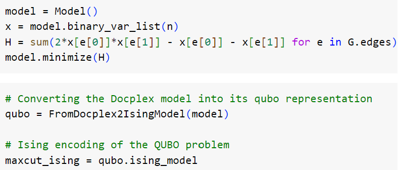
Figure 11: Creating the Max-Cut QUBO model

5.2.1 OpenQAOA Circuit

Once the QUBO is created, OpenQAOA provides an extremely short and easy implementation to create the QAOA circuit. Through a few lines of code, the user can define the backend device, backend properties, circuit type, circuit repetition, and optimizer. They then compile the QUBO and optimize the circuit for it to output optimal results.

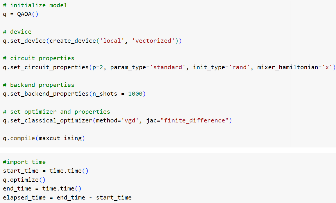
Figure 12: Creating the OpenQAOA circuit

5.2.2 Analysis Tools

Once the circuit is created, various visualization tools can be instantly implemented. After post-processing the most common output bitstring to obtain the Max-Cut graph, we obtain the optimal partition graph for the Maximum Cut.

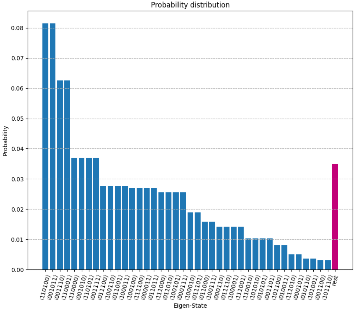
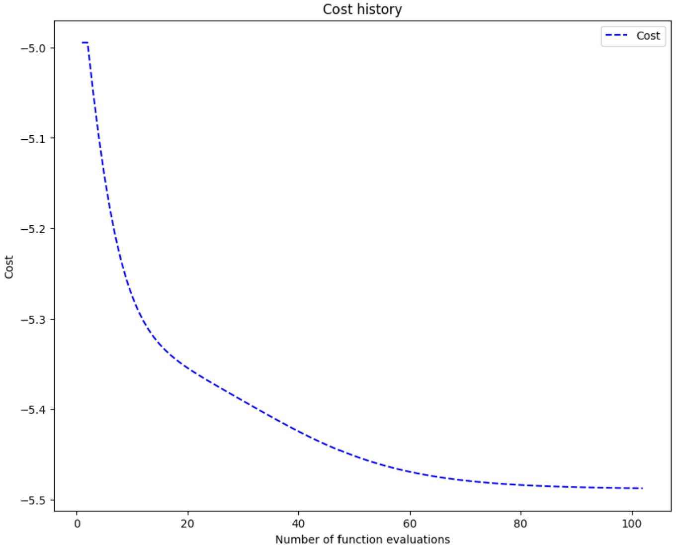
Figure 13: Probability Distribution of all Solution Bitstrings

Figure 14: Optimization Plot

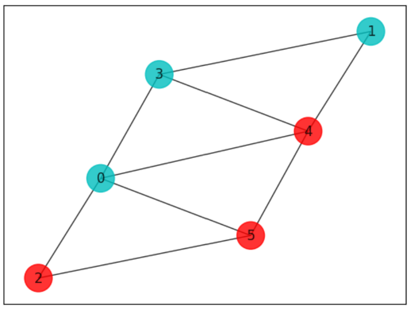
Figure 15: Optimal Graph Partitioning (Max Cut) based on Most Common Bitstring: (Nodes 2, 4 and 5) and Nodes (0, 1, 3)

5.3 QAOA via Qiskit

Qiskit-Optimization is a part of IBM Qiskit’s open-source quantum computing framework. It provides easy high-level applications of quantum algorithms that can run on both classical and quantum simulators. It provides a wide array of algorithms and built-in application classes for many canonical problems.

Qiskit Optimization is an extremely useful and easy way to solve QUBOs with various quantum algorithms including Variational Quantum Eigensolver [21], Adaptive Grover [11], and QAOA. Furthermore, because of compatibility with IBMQ, algorithms can run on actual IBM quantum backends. In the examples below, all code is run by default on the Qiskit QASM simulator. Although base-level implementation is easier, customization and in-depth analysis in more difficult. Tasks like plotting optimization history or bitstring distributions, although possible, are significantly more challenging. Qiskit-Optimization’s key limitations are its extremely long optimization times and limited set of optimizers.

Let us now consider the Minimum Vertex Cover problem. The first step is to create a problem instance and its corresponding QUBO model.

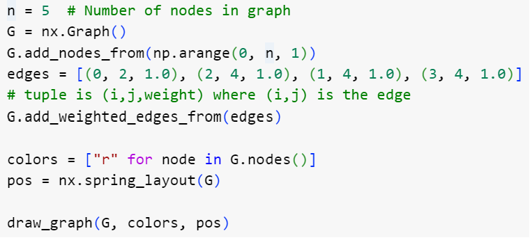
Figure 16: Creating a Minimum Vertex Cover instance

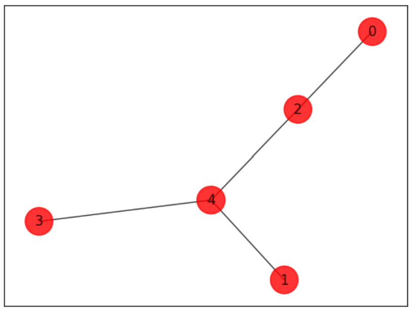
Figure 17: Generated graph instance

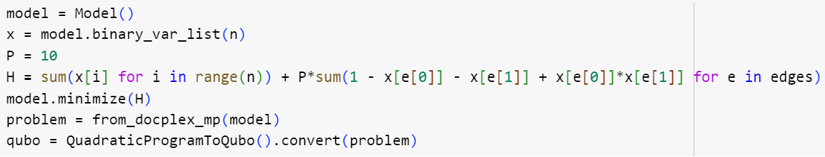
Figure 18: Creating the Minimum Vertex Cover QUBO

Similar to the Vanilla and OpenQAOA implementations, the following steps are to set up the QAOA circuit and optimize it. Because of the built-in capabilities of the Qiskit-Optimization, this requires very little extra effort.

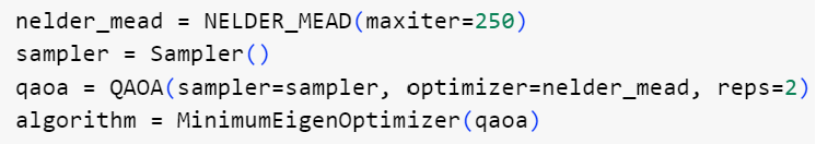
Figure 19: Creating the Minimum Vertex Cover QAOA circuit

Thus we obtain the following solution Minimum Vertex Cover graph.

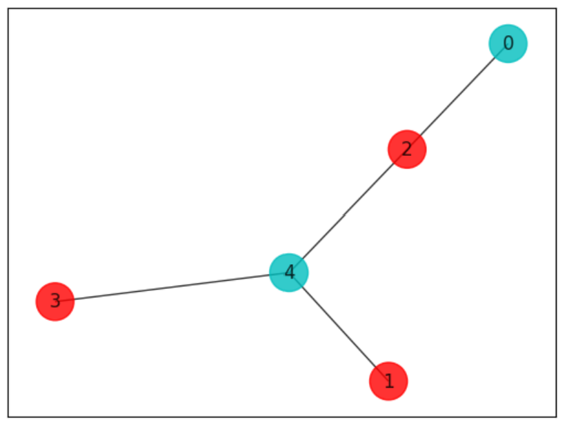
Figure 20: Optimal Minimum Vertex Cover: Nodes 0 and 4

5.4 Quantum Annealing

Let us now turn to Quantum Annealing. This algorithm was implemented using D-Wave’s Quantum Annealer and is applied to the Cancer Genomics application. Due to the higher number of qubits available here (as compared to IBM devices), larger instances can be executed.

The Cancer Genomics problem requires significant preprocessing effort. First, to construct the cancer pathway QUBO, the disease data must be read from some external source. For this tutorial, the data was collected from The Cancer Genome Atlas Acute Myeloid Leukemia dataset posted on cBioPortal [16].

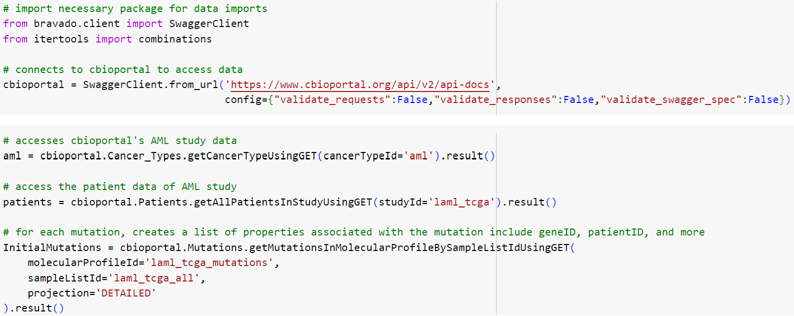
Figure 21: Reading TCGA-LAML data from cBioPortal

Using this data, a Patient-Gene dictionary is constructed similar to the one shown below:

Figure 22: Patient-Gene Dictionary example

With this dictionary, a diagonal matrix $\mathbf{D}$ is created where index $d_{ii}$ of $\mathbf{D}$ represents the number of instances of gene $i$ amongst the patients.

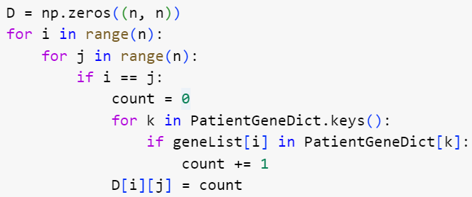
Figure 23: Creation of Diagonal Matrix $\mathbf{D}$ using the Patient-Gene dictionary

To create the $\mathbf{A}$ weighted adjacency matrix, the Patient-Gene dictionary is modified to contain Gene Pairs. This new Patient-Gene Pair dictionary is then used to create the adjacency $\mathbf{A}$ matrix.

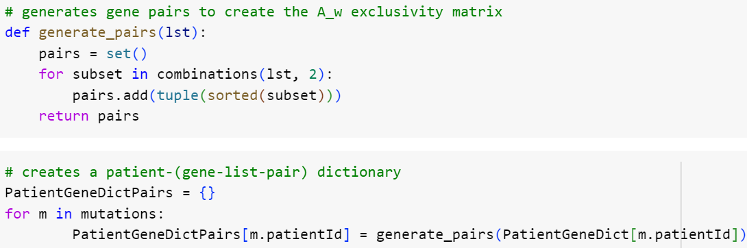
Figure 24: Code to create the dictionary of Patients and Gene-Pairs

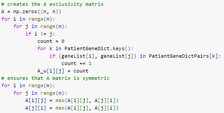
Figure 25: Creation of Adjacency Matrix $\mathbf{A}$ using the Patient-Gene-Pair dictionary

Once the $\mathbf{D}$ and $\mathbf{A}$ matrices are constructed, we create the QUBO model and later the Binary Quadratic Model (BQM) to run on D-Wave. This BQM is unconstrained as uses binary unconstrained variables to model.

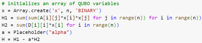
Figure 26: Creation of Cancer QUBO using $\mathbf{D}$ and $\mathbf{A}$ matrices

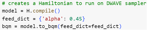
Figure 27: Creation of Cancer BQM from the QUBO

Once the BQM is created, it is then mapped to the qubits on the Quantum Processing Unit (QPU). Recall the original form of a QUBO model:

$$\sum_{i<j}Q_{ij}x_{i}x_{j}+\sum_{i}Q_{ii}x_{i}.$$

This can be mapped to a graph where $Q_{ii}$ is the bias of the nodes and $Q_{ij}$ is the weight of the edges. This mapping from the binary quadratic model to the QPU graph is known as minor embedding, and typically the Ocean API does this step automatically. After this, the actual Quantum Annealing process begins.

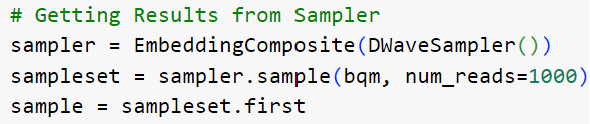
Figure 28: Running the Cancer Hamiltonian on the DWAVE Sampler

The annealing process will return multiple outputs, so we call ”sample first” to return the one with the lowest energy. Typically the variables are unordered so they must be sorted to correspond correctly to the genes.

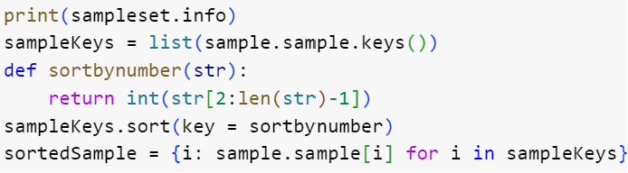
Figure 29: Sorting the QUBO output, to return the correct genes

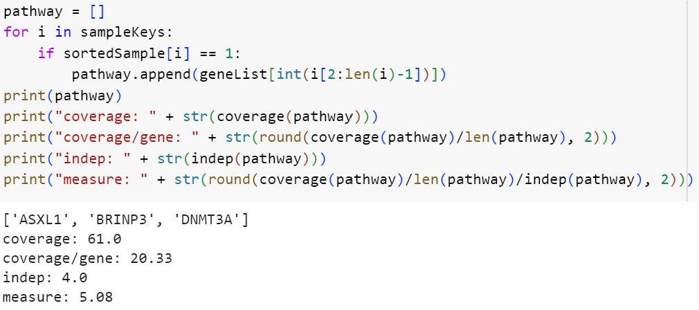
Figure 30: Example of mapping from Binary Solution to Genes

5.5 Simulated Annealing

The final algorithm we cover is Simulated Annealing for Order Partitioning. Like the other algorithms, the first step is to create the problem instance.

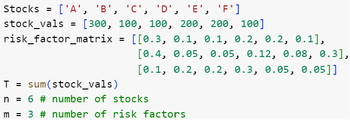
Figure 31: Order Partitioning Problem instance

The next step is to construct the problem QUBO.

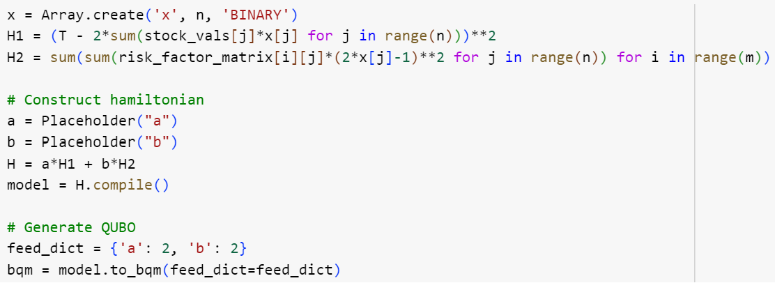
Figure 32: Order Partitioning QUBO from risk factor matrix and stock values

Once the Order Partitioning BQM is created, it is then run on the Simulated Annealing Sampler.

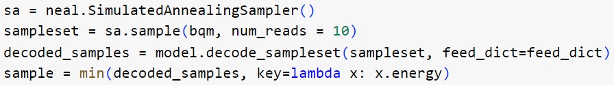
Figure 33: Order Partitioning using Simulated Annealing

The binary solution is then sorted and the output can be printed.

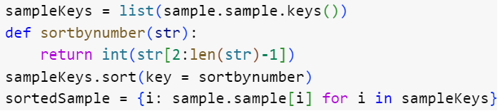
Figure 34: Sorting the Output from Simulated Annealing Sampler

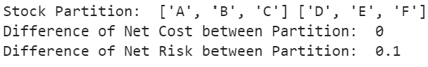
Figure 35: Solution to Order Partitioning instance

6 Concluding Remarks

The purpose of this tutorial was to rapidly introduce to a novice how to (a) represent canonical and practical problems as Quadratic Unconstrained Binary Optimization (QUBO) models and (b) solve them using both (i) Gate/Circuit quantum computers (such as IBM) using Quantum Approximate Optimization Algorithm (QAOA), (ii) Quantum Annealing (on D-Wave) and (iii) Simulated Annealing (classical). We illustrated the above algorithms on three canonical problems - Number Partitioning, Max-Cut, and Minimum Vertex Cover - and two practical problems, one from cancer genomics and the other from a Hedge Fund portfolio manager [25]. To take fuller advantage of these nascent devices, it is necessary to develop decomposition methods, an active area of research [26], and a topic for a future tutorial.

Acknowledgements. The authors thank Claudio Gomes, Anil Prabhakar, Elias Towe, and Shrinath Viswanathan for their comments on the previous version.

References

- [1] Hedayat Alghassi, Raouf Dridi, A. Gordon Robertson, and Sridhar Tayur. Quantum and quantum-inspired methods for de novo discovery of altered cancer pathways. bioRxiv, 2019.
- [2] Amazon Web Services. Amazon Braket, 2020.
- [3] Various authors. Qiskit Textbook. Github, 2023.
- [4] David E. Bernal, Sridhar Tayur, and Davide Venturelli. Quantum Integer Programming (QuIP) 47-779: Lecture Notes, 2021.
- [5] Zhengbing Bian, Fabian Chudak, Robert Brian Israel, Brad Lackey, William G. Macready, and Aidan Roy. Mapping constrained optimization problems to quantum annealing with application to fault diagnosis. Frontiers in ICT, 3, 2016.
- [6] Jianer Chen, Iyad A. Kanj, and Ge Xia. Improved parameterized upper bounds for Vertex Cover. In Mathematical Foundations of Computer Science 2006, pages 238–249, Berlin, Heidelberg, 2006. Springer Berlin Heidelberg.
- [7] Clayton W. Commander. Maximum cut problem, MAX-CUT, pages 1991–1999. Springer US, Boston, MA, 2009.
- [8] IBM ILOG Cplex. V12. 1: User’s manual for cplex. International Business Machines Corporation, 46(53):157, 2009.
- [9] Diego de Falco and Dario Tamascelli. An introduction to quantum annealing. RAIRO - Theoretical Informatics and Applications, 45, 07 2011.
- [10] Edward Farhi, Jeffrey Goldstone, and Sam Gutmann. A quantum approximate optimization algorithm, 2014.
- [11] Austin Gilliam, Stefan Woerner, and Constantin Gonciulea. Grover adaptive search for constrained polynomial binary optimization. Quantum, 5:428, April 2021.
- [12] Fred Glover, Jin-Kao Hao, Gary Kochenberger, Mark Lewis, Zhipeng Lu, Haibo Wang, Yang Wang, Haibo Wang, and Yang Wang. The unconstrained binary quadratic programming problem: a survey. Journal of Combinatorial Optimization, 28:58 – 81, 2014.
- [13] Johnny Hooyberghs. Azure Quantum, pages 307–339. Apress, Berkeley, CA, 2022.
- [14] Peter J Karalekas, Nikolas A Tezak, Eric C Peterson, Colm A Ryan, Marcus P da Silva, and Robert S Smith. A quantum-classical cloud platform optimized for variational hybrid algorithms. Quantum Science and Technology, 5(2):024003, April 2020.
- [15] S. Kirkpatrick, C. D. Gelatt, and M. P. Vecchi. Optimization by simulated annealing. Science, 220(4598):671–680, 1983.
- [16] Timothy J. Ley, Christopher B. Miller, Li xia Ding, Benjamin J. Raphael, Andrew J. Mungall, A. Gordon Robertson, Katherine A. Hoadley, Timothy J. Triche, Peter W. Laird, J. David Baty, Lucinda L. Fulton, Robert S. Fulton, Sharon E. Heath, Joelle M. Kalicki-Veizer, Cyriac Kandoth, Jeffery M. Klco, Daniel C. Koboldt, Krishna L. Kanchi, Shashikant Kulkarni, Tamara L. Lamprecht, David E. Larson, Ling Lin, Charles Lu, Michael D. McLellan, Joshua F. McMichael, Jacqueline E. Payton, Heather K. Schmidt, David H. Spencer, Michael H. Tomasson, John W. Wallis, Lukas D Wartman, Mark A. Watson, John S S Welch, Michael C. Wendl, Adrian Ally, Miruna Balasundaram, Inanç Birol, Yaron S. N. Butterfield, Readman Chiu, Andy Chu, Eric Chuah, Hye-Jung E. Chun, Richard Corbett, Noreen Dhalla, Ranabir Guin, Ann He, Carrie Hirst, Martin Hirst, Robert A. Holt, Steven P. Jones, Aly Karsan, Darlene Lee, Haiyan Irene Li, Marco A. Marra, Michael Mayo, Richard A. Moore, Karen L. Mungall, Jeremy D.K. Parker, Erin D. Pleasance, Patrick Plettner, Jacquie E. Schein, Dominik Stoll, Lucas Swanson, Angela Tam, Nina Thiessen, Richard Varhol, Natasja H. Wye, Yongjun Zhao, S. Gabriel, Gad Getz, Carrie Sougnez, Lihua Zou, Mark D. M. Leiserson, Fabio Vandin, Hsin-Ta Wu, Frederick R. Applebaum, Stephen B. Baylin, Rehan Akbani, Bradley M. Broom, Ken Chen, Thomas C. Motter, Khanh Nguyen, John N. Weinstein, Nianziang Zhang, Martin L. Ferguson, Christopher Adams, Aaron D. Black, Jay Bowen, Julie M. Gastier-Foster, Tom Grossman, Tara M. Lichtenberg, Lisa Wise, Tanja Davidsen, John A. Demchok, Kenna R. Mills Shaw, Margi Sheth, Heidi J. Sofia, Liming Yang, James R. Downing, and Greg D. Eley. Genomic and epigenomic landscapes of adult de novo acute myeloid leukemia. The New England journal of medicine, 368 22:2059–74, 2013.
- [17] Andrew Lucas. Ising formulations of many NP problems. Frontiers in Physics, 2, 2014.
- [18] Catherine C McGeoch. Adiabatic Quantum Computation and Quantum Annealing. Morgan&Claypool, Kenfield, CA, 2014.
- [19] Stephan Mertens. Phase transition in the number partitioning problem. Phys. Rev. Lett., 81:4281–4284, Nov 1998.
- [20] M. A. Nielsen and I. L. Chuang. Quantum Computation and Quantum Information: 10th Anniversary Edition. Cambridge University Press, New York, NY, USA, 2011.
- [21] Alberto Peruzzo, Jarrod McClean, Peter Shadbolt, Man-Hong Yung, Xiao-Qi Zhou, Peter J. Love, Alán Aspuru-Guzik, and Jeremy L. O’Brien. A variational eigenvalue solver on a photonic quantum processor. Nature Communications, 5(1), July 2014.
- [22] Qiskit contributors. Qiskit: An open-source framework for quantum computing, 2023.
- [23] Eleanor Rieffel and Wolfgang Polak. Quantum Computing: A Gentle Introduction. The MIT Press, Cambridge, MA, 2014.
- [24] Vishal Sharma, Nur Shahidee Bin Saharan, Shao-Hen Chiew, Ezequiel Ignacio Rodríguez Chiacchio, Leonardo Disilvestro, Tommaso Federico Demarie, and Ewan Munro. Openqaoa – an sdk for qaoa, 2022.
- [25] ManMohan S. Sodhi and Sridhar R. Tayur. Make Your Business Quantum-Ready Today. Management and Business Review, 2023.
- [26] Sridhar Tayur and Ananth Tenneti. Quantum Annealing Research at CMU: Algorithms, Hardware, Applications. Frontiers of Computer Science, 2024.