Cascading Reinforcement Learning

Abstract

Cascading bandits have gained popularity in recent years due to their applicability to recommendation systems and online advertising. In the cascading bandit model, at each timestep, an agent recommends an ordered subset of items (called an item list) from a pool of items, each associated with an unknown attraction probability. Then, the user examines the list, and clicks the first attractive item (if any), and after that, the agent receives a reward. The goal of the agent is to maximize the expected cumulative reward. However, the prior literature on cascading bandits ignores the influences of user states (e.g., historical behaviors) on recommendations and the change of states as the session proceeds. Motivated by this fact, we propose a generalized cascading RL framework, which considers the impact of user states and state transition into decisions. In cascading RL, we need to select items not only with large attraction probabilities but also leading to good successor states. This imposes a huge computational challenge due to the combinatorial action space. To tackle this challenge, we delve into the properties of value functions, and design an oracle $\mathtt{BestPerm}$ to efficiently find the optimal item list. Equipped with $\mathtt{BestPerm}$, we develop two algorithms $\mathtt{CascadingVI}$ and $\mathtt{CascadingBPI}$, which are both computationally-efficient and sample-efficient, and provide near-optimal regret and sample complexity guarantees. Furthermore, we present experiments to show the improved computational and sample efficiencies of our algorithms compared to straightforward adaptations of existing RL algorithms in practice.

1 Introduction

In recent years, a model called cascading bandits (Kveton et al., 2015a; Combes et al., 2015; Li et al., 2016; Vial et al., 2022) has received extensive attention in the online learning community, and found various applications such as recommendation systems (Mary et al., 2015) and online advertising (Tang et al., 2013). In this model, an agent is given a ground set of items, each with an unknown attraction probability. At each timestep, the agent recommends an ordered list of items to a user, and the user examines the items one by one, where the probability that each item attracts the user is equal to its attraction probability. Then, the user clicks the first attractive item (if any), and skips the following items. If an item is clicked in the list, the agent receives a reward; if no item is clicked, the agent receives no reward. The objective of the agent to maximize the expected cumulative reward.

While the cascading bandit model has been extensively studied, it neglects the influences of user states (e.g., characteristics and historical behaviors) on recommendations, and the fact that states can transition as users take actions. For example, in personalized video recommendation, the recommendation system usually suggests a list of videos according to the characteristics and viewing records of users. If the user clicks a video, the environment of the system can transition to a next state that stores the user’s latest behavior and interest. Next, the recommendation system will suggest videos of a similar type as what the user watched before to improve the click-through rate.

To model such state-dependent behavior, we propose a novel framework called cascading reinforcement learning (RL), which generalizes the conventional cascading bandit model to depict the influences of user states on recommendations and the transition of states in realistic applications. In this framework, there is a pool of $N$ items and a space of states. Each state-item pair is associated with an unknown attraction probability, an underlying transition distribution and a deterministic reward. In each episode (e.g., a session in recommendation systems), at each step, the agent first observes the current state (e.g., user characteristics and historical behaviors), and recommends a list of at most $m\leq N$ items. Then, the user (environment) goes over the list one by one, and clicks the first interesting item. After that, the agent receives a reward and transitions to a next state according to the current state and clicked item. If no item in the list interests the user, the agent receives zero reward and transitions to a next state according to the current state and a virtual item $a_{\bot}$. Here we say that the user clicks $a_{\bot}$ if no item is clicked. We define a policy as a mapping from the space of states and the current step to the space of item lists, and the optimal policy as the policy that maximizes the expected cumulative reward. Under this framework, we investigate two popular objectives in RL: minimizing the regret (i.e., the difference in rewards compared to always taking the optimal policy), and identifying a near-optimal policy.

This cascading RL framework faces a significant computational challenge. In conventional cascading bandits, there is no state, and the optimal policy is just to select $m$ items with the largest attraction probabilities. By contrast, in cascading RL, states also matter, which means that we need to balance between the maximization of the attraction probabilities of chosen items and the optimization of the expected reward that can be obtained in future states. This poses a great computational difficulty in the planning of the optimal policy under the combinatorial action space. Moreover, the combinatorial action space also brings a challenge on sample efficiency, i.e., how to avoid a dependency on the exponential number of actions in sample complexity.

To handle these challenges, we conduct a fine-grained analysis on the properties of value functions, and design an efficient oracle $\mathtt{BestPerm}$ to find the optimal item list, based on a novel dynamic programming for combinatorial optimization. Furthermore, we propose computationally and sample efficient algorithms $\mathtt{CascadingVI}$ and $\mathtt{CascadingBPI}$, which employ oracle $\mathtt{BestPerm}$ to only maintain the estimates for items and avoid enumerating over item lists. Our algorithms achieve polynomial regret and sample complexity in all problem parameters, and are near-optimal up to factor $H$. Finally, we also conduct experiments to demonstrate the superiority of our algorithms over naive adaptations of classic RL algorithms in computation and sampling.

The contributions of this work are summarized as follows.

• We propose the cascading RL framework, which generalizes the traditional cascading bandit model to formulate the influences of user states (e.g., historical behaviors) on recommendations and the change of states through time. This framework can be applied to various real-world scenarios, e.g., personalized recommendation systems and online advertising.

• To tackle the computational challenge of cascading RL, we leverage the properties of value functions to develop a novel oracle $\mathtt{BestPerm}$, which uses a carefully-designed dynamic programming to efficiently find the optimal item list under combinatorial action spaces.

• For the regret minimization objective, with oracle $\mathtt{BestPerm}$, we design an efficient algorithm $\mathtt{CascadingVI}$, and establish a $\tilde{O}(H\sqrt{HSNK})$ regret, which matches a known lower bound up to a factor of $\tilde{O}(\sqrt{H})$. Here $S$ is the number of states, $H$ is the length of each episode and $K$ is the number of episodes. Note that the regret depends only on the number of items $N$, instead of the total number of item lists, which is exponential.

• For the best policy identification objective, we devise a computationally and sample efficient algorithm $\mathtt{CascadingBPI}$, and provide $\tilde{O}(\frac{H^{3}SN}{\varepsilon^{2}})$ sample complexity. $\mathtt{CascadingBPI}$ is optimal up to a factor of $\tilde{O}(H)$ when $\varepsilon$ is small enough, where $\varepsilon$ is an accuracy parameter.

2 Related Work

In this section, we briefly review two lines of related works.

Cascading bandits. Kveton et al. (2015a) and Combes et al. (2015) concurrently introduce the cascading bandit model, and design algorithms based on upper confidence bounds with gap-dependent regret analysis. Following these works, Kveton et al. (2015b); Katariya et al. (2016); Lagrée et al. (2016) and Zoghi et al. (2017) investigate cascading bandits with various different settings. Li et al. (2016); Zong et al. (2016) and Li & Zhang (2018) study cascading bandits with contextual environments and linear generalization. Cheung et al. (2019) and Zhong et al. (2021) design Thompson Sampling-based (Thompson, 1933) algorithms for cascading bandits, and establish gap-independent regret bounds. Vial et al. (2022) develop algorithms equipped with variance-aware confidence sets, and provide near-optimal gap-independent regret bounds.

Provably efficient RL. In recent years, there have been an emerging number of works that study RL with rigorous theoretical analysis for the regret minimization objective, e.g., (Jaksch et al., 2010; Agrawal & Jia, 2017; Azar et al., 2017; Jin et al., 2018; Zanette & Brunskill, 2019), and the best policy identification objective, e.g., (Dann & Brunskill, 2015; Dann et al., 2017; Kaufmann et al., 2021; Ménard et al., 2021). In contrast to the above works, we generalize cascading bandits to the RL framework to formulate the change of states (e.g., historical behaviors of users) through time, and better fit real-world recommendation and advertising applications.

3 Problem Formulation

In this section, we present the formulation of cascading RL.

We consider an episodic cascading Markov decision process (MDP) $\mathcal{M}(\mathcal{S},A^{\textup{ground}},\mathcal{A},m,q,p,r)$. Here $\mathcal{S}$ is the space of states. $A^{\textup{ground}}:=\{a_{1},\dots,a_{N},a_{\bot}\}$ is the ground set of items, where $a_{1},\dots,a_{N}$ are regular items and $a_{\bot}$ is a virtual item. Item $a_{\bot}$ is put at the end of each item list by default, which represents that no item in the list is clicked. An action (i.e., item list) $A$ is a permutation which consists of at least one and at most $m\leq N$ regular items and the item $a_{\bot}$ at the end. $\mathcal{A}$ is the collection of all actions. We use “action” and “item list” interchangeably throughout the paper. For any $A\in\mathcal{A}$ and $i\in[|A|]$, let $A(i)$ denote the $i$-th item in $A$, and we have $A(|A|)=a_{\bot}$.

For any $(s,a)\in\mathcal{S}\times A^{\textup{ground}}$, $q(s,a)\in[0,1]$ denotes the attraction probability, which gives the probability that item $a$ is clicked in state $s$; $r(s,a)\in[0,1]$ is the deterministic reward of clicking item $a$ in state $s$; $p(\cdot|s,a)\in\triangle_{\mathcal{S}}$ is the transition distribution, so that for any $s^{\prime}\in\mathcal{S}$, $p(s^{\prime}|s,a)$ gives the probability of transitioning to state $s^{\prime}$ if item $a$ is clicked in state $s$. For any $s\in\mathcal{S}$, we define $q(s,a_{\bot}):=1$ and $r(s,a_{\bot}):=0$ (because if no regular item is clicked, the agent must click $a_{\bot}$ and receives zero reward). Transition probability $p(\cdot|s,a_{\bot})$ allows to formulate an interesting scenario where the session ends if no item is clicked, by letting $p(s_{0}|s,a_{\bot})=1$ where $s_{0}$ is a special absorbing state that always induces zero reward. In addition, we define a deterministic policy $\pi=\{\pi_{h}:\mathcal{S}\mapsto\mathcal{A}\}_{h\in[H]}$ as a collection of $H$ mappings from the state space to the action space, so that $\pi_{h}(s)$ gives what item list to choose in state $s$ at step $h$.

The cascading RL game is as follows. In each episode $k$, an agent first chooses a policy $\pi^{k}$, and starts from a fixed initial state $s^{k}_{1}:=s_{1}$. At each step $h\in[H]$, the agent first observes the current state $s^{k}_{h}$ (e.g., stored historical behaviors of the user), and then selects an item list $A^{k}_{h}=\pi^{k}_{h}(s^{k}_{h})$ according to her policy. After that, the environment (user) browses the selected item list one by one following the order given in $A^{k}_{h}$. When the user browses the $i$-th item $A^{k}_{h}(i)$ ($i\in[|A^{k}_{h}|]$), there is a probability of $q(s^{k}_{h},A^{k}_{h}(i))$ that the user is attracted by the item and clicks the item. This attraction and clicking event is independent among all items. Once an item $A^{k}_{h}(i)$ is clicked, the agent observes which item is clicked and receives reward $r(s^{k}_{h},A^{k}_{h}(i))$, and transitions to a next state $s^{k}_{h+1}\sim p(\cdot|s^{k}_{h},A^{k}_{h}(i))$, skipping the subsequent items $\{A^{k}_{h}(j)\}_{i<j\leq|A^{k}_{h}|}$. On the other hand, if no regular item in $A^{k}_{h}$ is clicked, i.e., we say that $a_{\bot}$ is clicked, then the agent receives zero reward and transitions to a next state $s^{k}_{h+1}\sim p(\cdot|s^{k}_{h},a_{\bot})$. After step $H$, this episode ends and the agent enters the next episode.

For any $k>0$ and $h\in[H]$, we use $I_{k,h}$ to denote the index of the clicked item in $A^{k}_{h}$, and $I_{k,h}=|A^{k}_{h}|$ if no item is clicked. Similar to cascading bandits (Kveton et al., 2015a; Combes et al., 2015), in the cascading RL model the agent only observes the attraction of items $\{A^{k}_{h}(j)\}_{j\leq I_{k,h}}$ (i.e., items $\{A^{k}_{h}(j)\}_{j<I_{k,h}}$ are not clicked and item $A^{k}_{h}(i)$ is clicked), and the transition distribution associated with item $A^{k}_{h}(I_{k,h})$. Whether the user would click any item in $\{A^{k}_{h}(j)\}_{j>I_{k,h}}$ is unobserved.

For any policy $\pi$, $h\in[H]$ and $s\in\mathcal{S}$, we define value function $V^{\pi}_{h}:\mathcal{S}\mapsto[0,H]$ as the expected cumulative reward that can be obtained under policy $\pi$, starting from state $s$ at step $h$, till the end of the episode. Formally,

$$V^{\pi}_{h}(s)=\mathbb{E}_{q,p,\pi}\left[\sum_{h^{\prime}=h}^{H}r(s_{h^{\prime}},A_{h^{\prime}}(I_{h^{\prime}}))|s_{h}=s\right].$$

Similarly, for any policy $\pi$, $h\in[H]$ and $(s,A)\in\mathcal{S}\times\mathcal{A}$, we define Q-value function $Q^{\pi}_{h}:\mathcal{S}\times\mathcal{A}\mapsto[0,H]$ as the expected cumulative reward received under policy $\pi$, starting from $(s,A)$ at step $h$, till the end of the episode. Formally,

$$Q^{\pi}_{h}(s,A)=\mathbb{E}_{q,p,\pi}\left[\sum_{h^{\prime}=h}^{H}r(s_{h^{\prime}},A_{h^{\prime}}(I_{h^{\prime}}))|s_{h}=s,A_{h}=A\right].$$

Since $\mathcal{S}$, $\mathcal{A}$ and $H$ are finite, there exists a deterministic optimal policy $\pi^{*}$ which always gives the maximum value $V^{\pi^{*}}_{h}(s)$ for all $s\in\mathcal{S}$ and $h\in[H]$ (Sutton & Barto, 2018). The Bellman equation and Bellman optimality equation for cascading RL can be stated as follows.

$$\left\{\begin{aligned} Q^{\pi}_{h}(s,A)&=\sum_{i=1}^{|A|}\prod_{j=1}^{i-1}\Big{(}1-q(s,A(j))\Big{)}q(s,A(i))\Big{(}r(s,A(i))+p(\cdot|s,A(i))^{\top}V^{\pi}_{h+1}\Big{)}\\ V^{\pi}_{h}(s)&=Q^{\pi}_{h}(s,\pi_{h}(s))\\ V^{\pi}_{H+1}(s)&=0,\quad\forall s\in\mathcal{S},\end{aligned}\right.$$

$$\left\{\begin{aligned} Q^{*}_{h}(s,A)&=\sum_{i=1}^{|A|}\prod_{j=1}^{i-1}\Big{(}1-q(s,A(j))\Big{)}q(s,A(i))\Big{(}r(s,A(i))+p(\cdot|s,A(i))^{\top}V^{*}_{h+1}\Big{)}\\ V^{*}_{h}(s)&=\max_{A\in\mathcal{A}}Q^{*}_{h}(s,A)\\ V^{*}_{H+1}(s)&=0,\quad\forall s\in\mathcal{S}.\end{aligned}\right.$$ (1)

Here $\prod_{j=1}^{i-1}(1-q(s,A(j)))q(s,A(i))$ is the probability that item $A(i)$ is clicked, which captures the cascading feature. $r(s,A(i))+p(\cdot|s,A(i))^{\top}V^{*}_{h+1}$ is the expected cumulative reward received if item $A(i)$ is clicked. $Q^{*}_{h}(s,A)$ is the summation of the expected cumulative reward of each item in $A$.

We investigate two popular objectives in RL, i.e., regret minimization and best policy identification. In the regret minimization setting, the agent plays $K$ episodes with the goal of minimizing the regret

$$\mathcal{R}(K)=\sum_{k=1}^{K}V^{*}_{1}(s_{1})-V^{\pi^{k}}_{1}(s_{1}).$$

In the best policy identification setting, given a confidence parameter $\delta\in(0,1)$ and an accuracy parameter $\varepsilon$, the agent aims to identify an $\varepsilon$-optimal policy $\hat{\pi}$ which satisfies $V^{\hat{\pi}}_{1}(s_{1})\geq V^{*}_{1}(s_{1})-\varepsilon$ with probability at least $1-\delta$, using as few episodes as possible. Here the performance is measured by the number of episodes used, i.e., sample complexity.

4 An Efficient Oracle for Cascading RL

Input: $A^{\textup{ground}}$, $u:A^{\textup{ground}}\mapsto[0,1]$, $w:A^{\textup{ground}}\mapsto\mathbb{R}$.

1 Sort the items in $A^{\textup{ground}}$ in descending order of $w$, and denote the sorted sequence by $a_{1},\dots,a_{J},a_{\bot},a_{J+1},\dots,a_{N}$. Here $J$ denotes the number of items with weights above $w(a_{\bot})$;

2 if $J=0$ then

3       $a^{\prime}\leftarrow\operatornamewithlimits{argmax}_{a\in\{a_{1},\dots,a_{N}\}}\{u(a)w(a)+(1-u(a))w(a_{\bot})\}$; // Select the best single item

4       $S^{\textup{best}}\leftarrow(a^{\prime})$. $F^{\textup{best}}\leftarrow u(a^{\prime})w(a^{\prime})+(1-u(a^{\prime}))w(a_{\bot})$;

5      

6if $1\leq J\leq m$ then

7       $S^{\textup{best}}\leftarrow(a_{1},\dots,a_{J})$; // Simply output $(a_{1},\dots,a_{J})$

8       $F^{\textup{best}}\leftarrow\sum_{i=1}^{J}\prod_{j=1}^{i-1}(1-u(a_{j}))u(a_{i})w(a_{i})+\prod_{j=1}^{J}(1-u(a_{j}))w(a_{\bot})$;

9      

10if $J>m$ then

11       $S[J][1]\leftarrow(a_{J})$; // Select $m$ best items from $(a_{1},\dots,a_{J})$

12       $F[J][1]\leftarrow u(a_{J})w(a_{J})+(1-u(a_{J}))w(a_{\bot})$;

13       For any $i\in[J]$, $S[i][0]\leftarrow\emptyset$ and $F[i][0]\leftarrow w(a_{\bot})$;

14       For any $i\in[J]$ and $J-i+1<k\leq m$, $F[i][k]\leftarrow-\infty$;

15       for $i=J-1,J-2,\dots,1$ do

16             for $k=1,2,\dots,\min\{m,J-i+1\}$ do

17                   if $F[i+1][k]\geq w(a_{i})u(a_{i})+(1-u(a_{i}))F[i+1][k-1]$ then

18                         $S[i][k]\leftarrow S[i+1][k]$. $F[i][k]\leftarrow F[i+1][k]$;

19                        

20                  else

21                         $S[i][k]\leftarrow(a_{i},S[i+1][k-1])$;

22                         $F[i][k]\leftarrow u(a_{i})w(a_{i})+(1-u(a_{i}))F[i+1][k-1]$;

23                        

24                  

25            

26      $S^{\textup{best}}\leftarrow S[1][m]$. $F^{\textup{best}}\leftarrow F[1][m]$;

27      

28return $S^{\textup{best}},F^{\textup{best}}$;

Algorithm 1 $\mathtt{BestPerm}$: find $\operatornamewithlimits{argmax}_{A\in\mathcal{A}}f(A,u,w)$ and $\max_{A\in\mathcal{A}}f(A,u,w)$

In the framework of model-based RL, it is typically assumed that one has estimates (possibly including exploration bonuses) of the model, i.e., attraction and transition probabilities, and a planning problem is solved to compute the value functions. In our problem, this would correspond to solving the maximization in Eq. (1). Different from planning in classic RL (Jaksch et al., 2010; Azar et al., 2017; Sutton & Barto, 2018), a naive implementation of this maximization in cascading RL will incur exponential computation complexity due to the fact that we have to consider all $A\in\mathcal{A}$. In order to design efficient algorithms for cascading RL, we need to overcome this computational difficulty.

To tackle this difficulty, we note that each backward recursion step in Eq. (1) involves the solution of a discrete optimization problem of the following form: For any ordered subset of $A^{\textup{ground}}$ denoted by $A$, $u:A^{\textup{ground}}\mapsto\mathbb{R}$ and $w:A^{\textup{ground}}\mapsto\mathbb{R}$, define a weighted cascading reward function $f(A,u,w)$ as

$$f(A,u,w):=\sum_{i=1}^{|A|}\prod_{j=1}^{i-1}\Big{(}1-u(A(j))\Big{)}u(A(i))w(A(i)),$$

and we need to find

$$\max_{A\in\mathcal{A}}f(A,u,w).$$ (2)

Here $f(A,u,w)$ corresponds to $Q^{*}_{h}(s,A)$, $u(A(i))$ represents $q(s,A(i))$, and $w(A(i))$ stands for $r(s,A(i))+p(\cdot|s,A(i))^{\top}V^{*}_{h+1}$.

4.1 Crucial Properties of Problem (2)

Before introducing an efficient oracle to solve problem Eq. (2), we first exhibit several nice properties of this optimization problem, which serve as the foundation of our oracle design.

For any subset of items $X\subseteq A^{\textup{ground}}$, let $\textup{Perm}(X)$ denote the collection of permutations of the items in $X$, and $\textup{DesW}(X)\in\textup{Perm}(X)$ denote the permutation where items are sorted in descending order of $w$. For convenience of analysis, here we treat $a_{\bot}$ as an ordinary item as $a_{1},\dots,a_{N}$, and $a_{\bot}$ can appear in any position in the permutations in $\textup{Perm}(X)$.

Lemma 1.

The weighted cascading reward function $f(A,u,w)$ satisfies the following properties:

1. For any $u$, $w$ and $X\subseteq A^{\textup{ground}}$, we have

   $$f(\textup{DesW}(X),u,w)=\max_{A\in\textup{Perm}(X)}f(A,u,w).$$

2. For any $u$, $w$ and disjoint $X,X^{\prime}\subseteq A^{\textup{ground}}\setminus\{a_{\bot}\}$ such that $w(a)>w(a_{\bot})$ for any $a\in X,X^{\prime}$, we have

   $$f((\textup{DesW}(X),a_{\bot}),u,w)\leq f((\textup{DesW}(X\cup X^{\prime}),a_{\bot}),u,w).$$

   Furthermore, for any $u$, $w$ and disjoint $X,X^{\prime}\subseteq A^{\textup{ground}}\setminus\{a_{\bot}\}$ such that $w(a)>w(a_{\bot})$ for any $a\in X$, and $w(a)<w(a_{\bot})$ for any $a\in X^{\prime}$, we have

   $$f((\textup{DesW}(X,X^{\prime}),a_{\bot}),u,w)\leq f((\textup{DesW}(X),a_{\bot}),u,w).$$

Property (i) can be proved by leveraging the continued product structure in $f(A,u,w)$ and a similar analysis as the interchange argument (Bertsekas & Castanon, 1999; Ross, 2014). Property (ii) follows from property (i) and the fact that $u(a_{\bot})=1$. The detailed proofs are presented in Appendix B.

Remark.

Property (i) exhibits that when fixing a subset of $A^{\textup{ground}}$, the best order of this subset is to rank items in descending order of $w$. Then, the best permutation selection problem in Eq. (2) can be reduced to a best subset selection problem.

Then, a natural question is what items and how many items should the best subset (permutation) include? Property (ii) gives an answer —– we should include the items with weights above $w(a_{\bot})$, and discard the items with weights below $w(a_{\bot})$. The intuition behind is as follows: If a permutation does not include the items in $X^{\prime}$ such that $w(a)>w(a_{\bot})$ for any $a\in X^{\prime}$, this is equivalent to putting $X^{\prime}$ behind $a_{\bot}$, since $u(a_{\bot})=1$. Then, according to property (i), we can arrange the items in $X^{\prime}$ in front of $a_{\bot}$ (i.e., include them) to obtain a better permutation. Similarly, if a permutation includes the items $X^{\prime}$ such that $w(a)<w(a_{\bot})$ for any $a\in X^{\prime}$, from property (i), we can also obtain a better permutation by putting $X^{\prime}$ behind $a_{\bot}$, i.e., discarding them.

4.2 Oracle $\mathtt{BestPerm}$

Making use of the properties of $f(A,u,w)$, we develop an efficient oracle $\mathtt{BestPerm}$ to solve problem Eq. (2), based on a carefully-designed dynamic programming to find the optimal item subset.

Algorithm 1 presents the pseudo-code of oracle $\mathtt{BestPerm}$. Given attraction probabilities $u$ and weights $w$, we first sort the items in $A^{\textup{ground}}$ in descending order of $w$, and denote the sorted sequence by $a_{1},\dots,a_{J},a_{\bot},a_{J+1},\dots,a_{N}$. Here $J$ denotes the number of items with weights above $w(a_{\bot})$. If $J=0$, i.e., $a_{\bot}$ has the highest weight, since the solution must contain at least one item, we choose the best single item as the solution (lines 1-1). If $1\leq J\leq m$, $(a_{1},\dots,a_{J})$ just satisfies the cardinality constraint and is the best permutation (lines 1-1). If $J>m$, to meet the cardinality constraint, we need to select $m$ best items from $(a_{1},\dots,a_{J})$ which maximize the objective value, i.e.,

$$\max_{(a^{\prime}_{1},\dots,a^{\prime}_{m})\subseteq(a_{1},\dots,a_{J})}f((a^{\prime}_{1},\dots,a^{\prime}_{m}),u,w).$$ (3)

Eq. (3) is a challenging combinatorial optimization problem, and costs exponential computation complexity if one performs naive exhaustive search. To solve Eq. (3), we resort to dynamic programming. For any $i\in[J]$ and $k\in[\min\{m,J-i+1\}]$, let $S[i][k]$ and $F[i][k]$ denote the optimal solution and optimal value of the problem $\max_{(a^{\prime}_{1},\dots,a^{\prime}_{k})\subseteq(a_{i},\dots,a_{J})}f((a^{\prime}_{1},\dots,a^{\prime}_{k}),u,w)$. Utilizing the structure of $f(A,u,w)$, we have

$$\left\{\begin{aligned} F[J][1]&=u(a_{J})w(a_{J})+(1-u(a_{J}))w(a_{\bot}),\\ F[i][0]&=w(a_{\bot}),&1\leq i\leq J,\\ F[i][k]&=-\infty,&1\leq i\leq J,\ J-i+1<k\leq m,\\ F[i][k]&=\max\{F[i+1][k],\\ u(a_{i})&w(a_{i})+(1-u(a_{i}))F[i+1][k-1]\},&1\leq i\leq J-1,\ 1\leq k\leq\min\{m,J-i+1\}.\end{aligned}\right.$$

The idea of this dynamic programming is as follows. Consider that we want to select $k$ best items from $(a_{i},\dots,a_{J})$. If we put $a_{i}$ into the solution, we need to further select $k-1$ best items from $(a_{i+1},\dots,a_{J})$. In this case, we have $F[i][k]=u(a_{i})w(a_{i})+(1-u(a_{i}))F[i+1][k-1]$; Otherwise, if we do not put $a_{i}$ into the solution, we are just selecting $k$ best items from $(a_{i+1},\dots,a_{J})$, and then $F[i][k]=F[i+1][k]$. After computing this dynamic programming, we output $S[1][m]$ and $F[1][m]$ as the optimal solution and optimal value of Eq. (2) (lines 1-1). The proof of the correctness of $\mathtt{BestPerm}$ can be seen in Appendix B.

$\mathtt{BestPerm}$ achieves $O(Nm+N\log(N))$ computation complexity. This is dramatically better than the computation complexity of the naive exhaustive search, which is $O(|\mathcal{A}|)=O(N^{m})$, an exponential time in the the problem instance size.

5 Regret Minimization for Cascading RL

Input: $\delta$, $\delta^{\prime}:=\frac{\delta}{14}$, $L:=\log(\frac{KHSN}{\delta^{\prime}})$. For any $k>0$ and $s\in\mathcal{S}$, $\bar{q}^{k}(s,a_{\bot})=\underline{q}^{k}(s,a_{\bot})=q(s,a_{\bot}):=1$, $r(s,a_{\bot}):=0$ and $\bar{V}^{k}_{H+1}(s)=\underline{V}^{k}_{H+1}(s):=0$.

1 for $k=1,2,\dots,K$ do

2       for $h=H,H-1,\dots,1$ do

3             for $s\in\mathcal{S}$ do

4                   for $a\in A^{\textup{ground}}\setminus\{a_{\bot}\}$ do

5                         $b^{k,q}(s,a)\leftarrow\min\{2\sqrt{\frac{\hat{q}^{k}(s,a)(1-\hat{q}^{k}(s,a))L}{n^{k,q}(s,a)}}+\frac{5L}{n^{k,q}(s,a)},\ 1\}$;

6                         $\bar{q}^{k}(s,a)\leftarrow\hat{q}^{k}(s,a)+b^{k,q}(s,a)$. $\underline{q}^{k}(s,a)\leftarrow\hat{q}^{k}(s,a)-b^{k,q}(s,a)$;

7                        

8                  for $a\in A^{\textup{ground}}$ do

9                         $b^{k,pV}(s,a)\leftarrow\min\{2\sqrt{\frac{\textup{Var}_{s^{\prime}\sim\hat{p}^{k}}(\bar{V}^{k}_{h+1}(s^{\prime}))L}{n^{k,p}(s,a)}}\ +2\sqrt{\frac{\mathbb{E}_{s^{\prime}\sim\hat{p}^{k}}[(\bar{V}^{k}_{h+1}(s^{\prime})-\underline{V}^{k}_{h+1}(s^{\prime}))^{2}]L}{n^{k,p}(s,a)}}+\frac{5HL}{n^{k,p}(s,a)},\ H\}$;

10                         $\bar{w}^{k}(s,a)\leftarrow r(s,a)+\hat{p}^{k}(\cdot|s,a)^{\top}\bar{V}^{k}_{h+1}+b^{k,pV}(s,a)$;

11                        

12                  $\bar{V}^{k}_{h}(s),\ \pi^{k}_{h}(s)\leftarrow\mathtt{BestPerm}(A^{\textup{ground}},\bar{q}^{k}(s,\cdot),\bar{w}^{k}(s,\cdot)$);

13                   $\bar{V}^{k}_{h}(s)\leftarrow\min\{\bar{V}^{k}_{h}(s),\ H\}$. $A^{\prime}\leftarrow\pi^{k}_{h}(s)$;

14                   $\underline{V}^{k}_{h}(s)\leftarrow\max\{\sum_{i=1}^{|A^{\prime}|}\prod_{j=1}^{i-1}(1-\bar{q}^{k}(s,A^{\prime}(j)))\underline{q}^{k}(s,A^{\prime}(i))(r(s,A^{\prime}(i))+\hat{p}^{k}(\cdot|s,A^{\prime}(i))^{\top}\underline{V}^{k}_{h+1}-b^{k,pV}(s,A^{\prime}(i))),\ 0\}$;

15                  

16            

17      for $h=1,2,\dots,H$ do

18             Observe the current state $s^{k}_{h}$; // Take policy $\pi^{k}$ and observe the trajectory

19             Take action $A^{k}_{h}=\pi^{k}_{h}(s^{k}_{h})$. $i\leftarrow 1$;

20             while $i\leq m$ do

21                   Observe if $A^{k}_{h}(i)$ is clicked or not. Update $n^{k,q}(s^{k}_{h},A^{k}_{h}(i))$ and $\hat{q}^{k}(s^{k}_{h},A^{k}_{h}(i))$;

22                   if $A^{k}_{h}(i)$ is clicked then

23                         Receive reward $r(s^{k}_{h},A^{k}_{h}(i))$, and transition to a next state $s^{k}_{h+1}\sim p(\cdot|s^{k}_{h},A^{k}_{h}(i))$;

24                         $I_{k,h}\leftarrow i$. Update $n^{k,p}(s^{k}_{h},A^{k}_{h}(i))$ and $\hat{p}^{k}(\cdot|s^{k}_{h},A^{k}_{h}(i))$;

25                         break while; // Skip subsequent items

26                  else

27                         $i\leftarrow i+1$;

28                        

29                  

30            if $i=m+1$ then

31                   Transition to a next state $s^{k}_{h+1}\sim p(\cdot|s^{k}_{h},a_{\bot})$; // No item was clicked

32                   Update $n^{k,p}(s^{k}_{h},a_{\bot})$ and $\hat{p}^{k}(\cdot|s^{k}_{h},a_{\bot})$;

33                  

34            

35      

Algorithm 2 $\mathtt{CascadingVI}$

In this section, we study cascading RL with the regret minimization objective. Building upon oracle $\mathtt{BestPerm}$, we propose an efficient algorithm $\mathtt{CascadingVI}$, which is both computationally and sample efficient and has a regret bound that nearly matches the lower bound.

5.1 Algorithm $\mathtt{CascadingVI}$

$\mathtt{CascadingVI}$ is an optimistic value iteration-based algorithm, which only maintains the estimates for each item, instead of each item list, and adopts oracle $\mathtt{BestPerm}$ to directly calculate the value function $\bar{V}^{k}_{h}(s)$ and avoid computing $\bar{Q}^{k}_{h}(s,A)$ for each $A\in\mathcal{A}$.

Algorithm 2 describes $\mathtt{CascadingVI}$. In each episode $k$, we first calculate the optimistic attraction probability $\bar{q}^{k}(s,a)$ and weight $\bar{w}^{k}(s,a)$, by adding exploration bonuses for $q(s,a)$ and $p(\cdot|s,a)^{\top}V$ individually (lines 2 and 2). Here the weight $\bar{w}^{k}(s,a)$ represents an optimistic estimate of the expected cumulative reward that can be obtained if item $a$ is clicked in state $s$. Then, we invoke oracle $\mathtt{BestPerm}$ with $\bar{q}^{k}(s,\cdot)$ and $\bar{w}^{k}(s,\cdot)$ to efficiently compute the optimistic value function $\bar{V}^{k}_{h}(s)$ and its associated greedy policy $\pi^{k}_{h}(s)$ (line 2). This invocation of $\mathtt{BestPerm}$ takes advantage of the monotonicity property of $f(A,q,w)$, i.e., $f(A,\bar{q},w)\geq f(A,q,w)$ if $\bar{q}\geq q$ element-wise, which guarantees the optimism of $\bar{V}^{k}_{h}(s)$ (see detailed proofs in Appendix C.2.3).

After obtaining policy $\pi^{k}$, we play episode $k$ with $\pi^{k}$ (lines 2-2). At each step $h\in[H]$, we first observe the current state $s^{k}_{h}$, and select the item list $A^{k}_{h}=\pi^{k}_{h}(s)$. Then, the environment (user) examines the items in $A^{k}_{h}$ and clicks the first attractive item. Once an item $A^{k}_{h}(i)$ is clicked, the agent receives a reward and transitions to $s^{k}_{h+1}\sim p(\cdot|s^{k}_{h},A^{k}_{h}(i))$, skipping the subsequent items. If no item in $A^{k}_{h}$ is clicked, the agent receives zero reward and transitions to $s^{k}_{h+1}\sim p(\cdot|s^{k}_{h},a_{\bot})$.

If one naively adapts classical RL algorithms (Azar et al., 2012; Zanette & Brunskill, 2019) to solve cascading RL by treating each $A\in\mathcal{A}$ as an ordinary action, one will suffer a dependency on $|\mathcal{A}|$ in computation and sample complexities. By contrast, $\mathtt{CascadingVI}$ only maintains the estimates of attraction and transition probabilities for each $(s,a)$, and employs oracle $\mathtt{BestPerm}$ to directly compute $\bar{V}^{k}_{h}(s)$, without enumerating over $A\in\mathcal{A}$. Therefore, $\mathtt{CascadingVI}$ avoids the dependency on $|A|$ in computation and statistical complexities.

5.2 Theoretical Guarantee of Algorithm $\mathtt{CascadingVI}$

Now we investigate the regret guarantee for algorithm $\mathtt{CascadingVI}$.

In regret analysis, we first prove the monotonicity property of $f(A,u,w)$, which ensures the optimism of the value function $\bar{V}^{k}_{h}(s)$. Then, we establish a value difference lemma for cascading RL to decompose the regret into the estimation error of attraction and transition probabilities of each state-item pair. After that, we leverage the variance-awareness of exploration bonuses, and perform the summation of the estimation error over all state-item pairs to derive a regret bound. Specifically, the Bernstern’s construction $\hat{q}^{k}(s,a)(1-\hat{q}^{k}(s,a))$ in $b^{k,q}$ makes the estimation error adaptively dependent on $q$, which enables our regret bound to match the optimal result for cascading bandits (Vial et al., 2022) when the problem degenerates.

Theorem 1 (Regret Upper Bound).

With probability at least $1-\delta$, the regret of algorithm $\mathtt{CascadingVI}$ is bounded by

$$\tilde{O}\left(H\sqrt{HSNK}\right).$$

From Theorem 1, we see that the regret of $\mathtt{CascadingVI}$ depends only on the number of items $N$, instead of the number of item lists $|\mathcal{A}|=O(N^{m})$. This demonstrates the efficiency of our estimation scheme and exploration bonus design. When our problem degenerates to cascading bandits, i.e., $S=H=1$, our regret bound matches the optimal result for cascading bandits (Vial et al., 2022).

Lower bound and optimality.

Recall from (Jaksch et al., 2010; Osband & Van Roy, 2016) that the lower bound for classic RL is $\Omega(H\sqrt{SNK})$. Since cascading RL reduces to classic RL when $q(s,a)=1$ for any $(s,a)\in\mathcal{S}\times A^{\textup{ground}}$ (i.e., the user always clicks the first item), the lower bound $\Omega(H\sqrt{SNK})$ also holds for cascading RL.

Our regret bound matches the lower bound up to a factor of $\sqrt{H}$ when ignoring logarithmic factors. This gap comes from the fact that we add exploration bonuses for $q(s,a)$ and $p(\cdot|s,a)^{\top}V$ individually, and such scheme is not as tight as adding an exploration bonus for the whole transition distribution of $(s,A)$, i.e., consider the randomness from $q$ and $p$ as an integrated transition distribution of $(s,A)$. However, the latter strategy forces us to maintain the estimates for each $A\in\mathcal{A}$, and will incur a dependency on $|\mathcal{A}|$ in computation and statistical complexities. Therefore, how to close the gap $\sqrt{H}$ without enumerating over $A\in\mathcal{A}$ remains an open problem, which we leave for future work.

6 Best Policy Identification for Cascading RL

Now we turn to cascading RL with best policy identification. We propose an efficient algorithm $\mathtt{CascadingBPI}$ to find an $\varepsilon$-optimal policy. Here we mainly introduce the idea of $\mathtt{CascadingBPI}$, and defer the detailed pseudo-code and description to Appendix D.1 due to space limit.

In $\mathtt{CascadingBPI}$, we optimistically estimate $q(s,a)$ and $p(\cdot|s,a)^{\top}V$, and add exploration bonuses for them individually. Then, we call the oracle $\mathtt{BestPerm}$ to compute the optimistic value function and hypothesized optimal policy. Furthermore, we construct an estimation error to bound the deviation between the optimistic value function and true value function. If this estimation error shrinks within $\varepsilon$, we simply output the hypothesized optimal policy; Otherwise, we play an episode with this policy.

By only maintaining the estimates for each item and applying oracle $\mathtt{BestPerm}$, $\mathtt{CascadingBPI}$ also avoids calculating $Q^{k}_{h}(s,A)$ for each $A\in\mathcal{A}$. Hence, the computation complexity of $\mathtt{CascadingBPI}$ depends only on $N$, instead of $|\mathcal{A}|$, which is significantly better than an adaptation of classical best policy identification algorithms (Kaufmann et al., 2021; Ménard et al., 2021). In the following, we provide the sample complexity of $\mathtt{CascadingBPI}$.

Theorem 2.

With probability at least $1-\delta$, algorithm $\mathtt{CascadingBPI}$ returns an $\varepsilon$-optimal policy, and the number of episodes used is bounded by

$$\tilde{O}\left(\frac{H^{3}SN}{\varepsilon^{2}}\log\left(\frac{1}{\delta}\right)+\frac{H^{2}\sqrt{H}SN}{\varepsilon\sqrt{\varepsilon}}\left(\log\left(\frac{1}{\delta}\right)+S\right)\right),$$

where $\tilde{O}(\cdot)$ hides logarithmic factors with respect to $N,H,S$ and $\varepsilon$.

Theorem 2 reveals that the sample complexity of $\mathtt{CascadingBPI}$ is polynomial in problem parameters $N$, $H$, $S$ and $\varepsilon$, and independent of $|\mathcal{A}|$. Regarding the optimality, since cascading RL reduces to classic RL when $q(s,a)=1$ for all $(s,a)\in\mathcal{S}\times A^{\textup{ground}}$, existing lower bound for classic best policy identification $\Omega(\frac{H^{2}SN}{\varepsilon^{2}}\log(\frac{1}{\delta}))$ (Dann & Brunskill, 2015) also applies here. This corroborates that $\mathtt{CascadingBPI}$ is near-optimal up to a factor of $H$ when $\varepsilon$ is small enough.

7 Experiments

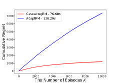
(a) Regret minimization, $N=4$

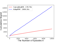
(b) Regret minimization, $N=8$

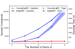
(c) Best policy identification

Figure 1: Experiments for cascading RL.

In this section, we present the experimental results for cascading RL. In our experiments, we set $\delta=0.005$, $H=5$, $S=9$ and $m=3$, and perform each algorithm for $20$ independent runs. In the regret minimization setting, we let $N\in\{4,8\}$ and $K=10000$, and show the average cumulative regrets and average running times (in the legend) across runs. In the best policy identification setting, we set $\epsilon=0.5$ and $N\in\{4,5,6,7,8\}$, and plot the average sample complexities and average running times across runs with $95\%$ confidence intervals.

Under the regret minimization objective, we compare our algorithm $\mathtt{CascadingVI}$ with an adaptation of a classical RL algorithm in (Zanette & Brunskill, 2019) to the combinatorial action space, named AdaptRM. From Figures 1(a) and 1(b), one can see that $\mathtt{CascadingVI}$ achieves significantly lower regret and running time than AdaptRM, and this advantage becomes more clear as $N$ increases. This result demonstrates the efficiency of our computation oracle and estimation scheme.

Regarding the regret minimization objective, we compare our algorithm $\mathtt{CascadingBPI}$ with AdaptBPI, an adaptation of a classic best policy identification algorithm in (Ménard et al., 2021) to combinatorial actions. In Figure 1(c), as $N$ increases, the sample complexity and running time of AdaptBPI increase exponentially fast. By contrast, $\mathtt{CascadingBPI}$ has much lower sample complexity and running time, and enjoys a mild growth rate as $N$ increases. This matches our theoretical result that the sample and computation complexities of $\mathtt{CascadingBPI}$ are polynomial in $N$.

8 Conclusion

In this work, we formulate a cascading RL framework, which generalizes the cascading bandit model to characterize the impacts of user states and state transition in applications such as recommendation systems. We design a novel oracle $\mathtt{BestPerm}$ to efficiently identify the optimal item list under combinatorial action spaces. Building upon this oracle, we develop efficient algorithms $\mathtt{CascadingVI}$ and $\mathtt{CascadingBPI}$ with near-optimal regret and sample complexity guarantees.

There are many future directions worth further investigation. One direction is to close the gap with respect to $H$ in our regret and sample complexity bounds. Another interesting direction is to extend our framework to the function approximation setting to allow infinite state and action spaces. A more general direction is to consider other combinatorial bandit problems that may also encounter state transition in real-world applications and extend them to the combinatorial RL setting.

Acnowledgement

The work of Yihan Du and R. Srikant is supported in part by AFOSR Grant FA9550-24-1-0002, ONR Grant N00014-19-1-2566, and NSF Grants CNS 23-12714, CNS 21-06801, CCF 19-34986, and CCF 22-07547.

Appendix

Appendix A Details of Experimental Setup

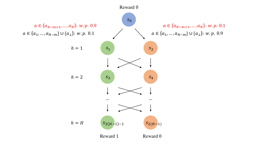
Figure 2: The instance in experiments.

In this section, we elaborate the details of experimental setup. In our experiments, we consider a cascading MDP with $H$ layers, $S=2H-1$ states and $N$ items as shown in Figure 2: There is only an initial state $s_{0}$ in the first layer. For any $2\leq h\leq H$, there are a good state $s_{2(h-1)-1}$ and a bad state $s_{2(h-1)}$ in layer $h$. The reward function depends only on states. All good states induce reward $1$, and all bad states and the initial state give reward $0$. The attraction probability for all state-item pairs is $\frac{1}{2}$. Denote $A^{\textup{ground}}=\{a_{1},\dots,a_{N}\}$. For any $h\in[H]$, under a good item $a\in\{a_{N-m+1},\dots,a_{N}\}$, the transition probabilities from each state in layer $h$ to the good state and the bad state in layer $h+1$ are $0.9$ and $0.1$, respectively. On the contrary, under a bad item $a\in\{a_{1},\dots,a_{N-m}\}\cup\{a_{\bot}\}$, the transition probabilities from each state in layer $h$ to the good state and the bad state in layer $h+1$ are $0.1$ and $0.9$, respectively. Therefore, in this MDP, an optimal policy is to select good items $(a_{N-m+1},\dots,a_{N})$ in all states.

The experiments are run on the Intel (R) Xeon (R) CPU E5-2678 v3 @ 2.50GHz with 16GB RAM, and each algorithm is performed for $20$ independent runs. In all experiments, we set $\delta=0.005$, $H=5$, $S=9$ and $m=3$. In the regret minimization setting, we let $N\in\{4,8\}$ and $K=10000$, and show the average cumulative regrets and average running times (in the legend) across runs. In the best policy identification setting, we set $\epsilon=0.5$ and $N\in\{4,5,6,7,8\}$, and plot the average sample complexities and average running times across runs with $95\%$ confidence intervals.

Appendix B Proofs for Oracle $\mathtt{BestPerm}$

In this section, we present the proofs for oracle $\mathtt{BestPerm}$.

First, we introduce two important lemmas which are used in the proof of Lemma 1.

Lemma 2 (Interchange by Descending Weights).

For any $u:A^{\textup{ground}}\mapsto[0,1]$, $w:A^{\textup{ground}}\mapsto\mathbb{R}$ and $A=(a_{1},\dots,a_{\ell},a_{\ell+1},\dots,a_{n})$ such that $1\leq\ell<n$ and $w(a_{\ell})<w(a_{\ell+1})$, denoting $A^{\prime}:=(a_{1},\dots,a_{\ell+1},a_{\ell},\dots,a_{n})$, we have

$$f(A,u,w)\leq f(A^{\prime},u,w).$$

Proof of Lemma 2.

This proof uses a similar idea as the interchange argument (Bertsekas & Castanon, 1999; Ross, 2014). We have

$$\quad\ f(A,u,w)-f(A^{\prime},u,w)$$

$$=\prod_{j=1}^{\ell-1}(1-u(a_{j}))\cdot\left(u(a_{\ell})w(a_{\ell})+(1-u(a_{\ell}))u(a_{\ell+1})w(a_{\ell+1})\right)$$

$$\quad\ -\prod_{j=1}^{\ell-1}(1-u(a_{j}))\cdot\left(u(a_{\ell+1})w(a_{\ell+1})+(1-u(a_{\ell+1}))u(a_{\ell})w(a_{\ell})\right)$$

$$=\prod_{j=1}^{\ell-1}(1-u(a_{j}))\cdot\left(u(a_{\ell+1})u(a_{\ell})w(a_{\ell})-u(a_{\ell})u(a_{\ell+1})w(a_{\ell+1})\right)$$

$$=\prod_{j=1}^{\ell-1}(1-u(a_{j}))\cdot u(a_{\ell})u(a_{\ell+1})\cdot\left(w(a_{\ell})-w(a_{\ell+1})\right)$$

$$\leq 0.$$

∎

Lemma 3 (Items behind $a_{\bot}$ Do Not Matter).

For any ordered subsets of $\{a_{1},\dots,a_{N}\}$, $A$ and $A^{\prime}$, such that $A\cap A^{\prime}=\emptyset$, we have

$$f((A,a_{\bot},A^{\prime}),u,w)=f((A,a_{\bot}),u,w).$$

Proof.

Since $u(a_{\bot})=1$, we have

$$f((A,a_{\bot},A^{\prime}),u,w)$$

$$= \sum_{i=1}^{|A|}\prod_{j=1}^{i-1}\Big{(}1-u(A(j))\Big{)}u(A(i))w(A(i))+\prod_{j=1}^{|A|}\Big{(}1-u(A(j))\Big{)}u(a_{\bot})w(a_{\bot})$$

$$+\sum_{i=1}^{|A^{\prime}|}\bigg{(}\prod_{\ell=1}^{|A|}\Big{(}1-u(A(\ell))\Big{)}\Big{(}1-u(a_{\bot})\Big{)}\prod_{j=1}^{i-1}\Big{(}1-u(A^{\prime}(j))\Big{)}\bigg{)}u(A^{\prime}(i))w(A^{\prime}(i))$$

$$= \sum_{i=1}^{|A|}\prod_{j=1}^{i-1}\Big{(}1-u(A(j))\Big{)}u(A(i))w(A(i))+\prod_{j=1}^{|A|}\Big{(}1-u(A(j))\Big{)}u(a_{\bot})w(a_{\bot})$$

$$= f((A,a_{\bot}),u,w).$$

∎

Now we prove Lemma 1.

For any $X\subseteq A^{\textup{ground}}$, let $\textup{Perm}(X)$ denote the collection of permutations of the items in $X$, and $\textup{DesW}(X)\in\textup{Perm}(X)$ denote the permutation where items are sorted in descending order of $w$.

Proof of Lemma 1.

First, we prove property (i) by contradiction.

Suppose that the best permutation $A^{*}=\operatornamewithlimits{argmax}_{A\in\textup{Perm}(X)}f(A,u,w)$ does not rank items in descending order of $w$. In other words, there exist some $a_{\ell},a_{\ell+1}$ such that we can write $A^{*}=(a_{1},\dots,a_{\ell},a_{\ell+1},\dots,a_{|X|})$ and $w(a_{\ell})<w(a_{\ell+1})$.

Then, using Lemma 2, we have that $A^{\prime}=(a_{1},\dots,a_{\ell+1},a_{\ell},\dots,a_{|X|})$ satisfies $f(A^{\prime},u,w)\geq f(A^{*},u,w)$, which contradicts the supposition. Given any permutation in $\textup{Perm}(X)$, we can repeatedly perform Lemma 2 to obtain a better permutation as bubble sort, until all items are ranked in descending order of $w$. Therefore, we obtain property (i).

Next, we prove property (ii).

For any $u$, $w$ and disjoint $X,X^{\prime}\subseteq A^{\textup{ground}}\setminus\{a_{\bot}\}$ such that $w(a)>w(a_{\bot})$ for any $a\in X,X^{\prime}$, we have

$$f((\textup{DesW}(X),a_{\bot}),u,w) \overset{\textup{(a)}}{=}f((\textup{DesW}(X),a_{\bot},X^{\prime}),u,w)$$

$$\overset{\textup{(b)}}{\leq}f((\textup{DesW}(X\cup X^{\prime}),a_{\bot}),u,w),$$

Here in the right-hand side of equality (a), $X^{\prime}$ can be in any order, and inequality (b) uses property (i).

Furthermore, for any $u$, $w$ and disjoint $X,X^{\prime}\subseteq A^{\textup{ground}}\setminus\{a_{\bot}\}$ such that $w(a)>w(a_{\bot})$ for any $a\in X$, and $w(a)<w(a_{\bot})$ for any $a\in X^{\prime}$, we have

$$f((\textup{DesW}(X,X^{\prime}),a_{\bot}),u,w) \overset{\textup{(c)}}{\leq}f((\textup{DesW}(X),a_{\bot},\textup{DesW}(X^{\prime})),u,w)$$

$$=f((\textup{DesW}(X),a_{\bot}),u,w),$$

where inequality (c) is due to property (i). ∎

Lemma 4 (Correctness of Oracle $\mathtt{BestPerm}$).

Given any $u:A^{\textup{ground}}\mapsto[0,1]$ and $w:A^{\textup{ground}}\mapsto\mathbb{R}$, the permutation $S^{\textup{best}}$ returned by algorithm $\mathtt{BestPerm}$ satisfies

$$f(S^{\textup{best}},u,w)=\max_{A\in\mathcal{A}}f(A,u,w).$$

Proof of Lemma 4.

From Lemma 1 (i), we have that when fixing a subset of $A^{\textup{ground}}$, the best order of this subset is to rank items in descending order of $w$. Thus, the problem of finding the best permutation in Eq. (2) reduces to finding the best subset, and then we can just sort items in this subset by descending $w$ to obtain the solution.

We sort the items in $A^{\textup{ground}}$ in descending order of $w$, and denote the sorted sequence by $a_{1},\dots,a_{J},a_{\bot},a_{J+1},\dots,a_{N}$. Here $J$ denotes the number of items with weights above $a_{\bot}$.

According to Lemma 1 (ii), we have that the best permutation only consists of items in $a_{1},\dots,a_{J}$. In other words, we should discard $a_{J+1},\dots,a_{N}$.

Case (i).

If $1\leq J\leq m$, $(a_{1},\dots,a_{J})$ satisfies the cardinality constraint and is the best permutation.

Case (ii).

Otherwise, if $J=0$, we have to select a single best item to satisfy that there is at least one regular item in the solution.

Why do not we select more items? We can prove that including more items gives a worse permutation by contradiction. Without loss of generality, consider a permutation with an additional item, i.e., $(a,a^{\prime},a_{\bot})$, where $a,a^{\prime}\in A^{\textup{ground}}\setminus\{a_{\bot}\}$ and $w(a),w(a^{\prime})<w(a_{\bot})$. Using Lemma 2, we have

$$f((a,a^{\prime},a_{\bot}),u,w) \leq f((a,a_{\bot},a^{\prime}),u,w)$$

$$=f((a,a_{\bot}),u,w).$$

In this case, the best permutation is the best single item $\operatornamewithlimits{argmax}_{a\in\{a_{1},\dots,a_{N}\}}f((a,a_{\bot}),u,w)$.

Case (iii).

If $J>m$, the problem reduces to selecting $m$ best items from $a_{1},\dots,a_{J}$. For any $i\in[J]$ and $k\in[\min\{m,J-i+1\}]$, let $F[i][k]$ denote the optimal value of the problem $\max_{(a^{\prime}_{1},\dots,a^{\prime}_{k})\subseteq(a_{i},\dots,a_{J})}f((a^{\prime}_{1},\dots,a^{\prime}_{k}),u,w)$. From the structure of $f(A,u,w)$, we have the following dynamic programming:

$$\left\{\begin{aligned} F[J][1]&=u(a_{J})w(a_{J})+(1-u(a_{J}))w(a_{\bot}),\\ F[i][0]&=w(a_{\bot}),&1\leq i\leq J,\\ F[i][k]&=-\infty,&1\leq i\leq J,\ J-i+1<k\leq m,\\ F[i][k]&=\max\{F[i+1][k],\\ u(a_{i})&w(a_{i})+(1-u(a_{i}))F[i+1][k-1]\},&1\leq i\leq J-1,\ 1\leq k\leq\min\{m,J-i+1\}.\end{aligned}\right.$$

Then, $F[1][m]$ gives the objective value of the best permutation.

Combining the above analysis, we have that $\mathtt{BestPerm}$ returns the best permutation, i.e., $f(S^{\textup{best}},u,w)=\max_{A\in\mathcal{A}}f(A,u,w)$. ∎

Appendix C Proofs for Cascading RL with Regret Minimization

In this section, we provide the proofs for cascading RL with the regret minimization objective.

C.1 Value Difference Lemma for Cascading MDP

We first give the value difference lemma for cascading MDP, which is useful for regret decomposition.

Lemma 5 (Cascading Value Difference Lemma).

For any two cascading MDPs $\mathcal{M}^{\prime}(\mathcal{S},A^{\textup{ground}},\mathcal{A},m,H,q^{\prime},p^{\prime},r^{\prime})$ and $\mathcal{M}^{\prime\prime}(\mathcal{S},A^{\textup{ground}},\mathcal{A},m,H,q^{\prime\prime},p^{\prime\prime},r^{\prime\prime})$, the difference in values under the same policy $\pi$ satisfies

$$V^{\prime\pi}_{h}(s)\! -\!V^{\prime\prime\pi}_{h}(s)=\sum_{t=h}^{H}\mathbb{E}_{q^{\prime\prime},p^{\prime\prime},\pi}\Bigg{[}\sum_{i=1}^{|A_{t}|}\prod_{j=1}^{i-1}(1-q^{\prime}(s_{t},A_{t}(j)))q^{\prime}(s_{t},A_{t}(i))r^{\prime}(s_{t},A_{t}(i))$$

$$-\sum_{i=1}^{|A_{t}|}\prod_{j=1}^{i-1}(1-q^{\prime\prime}(s_{t},A_{t}(j)))q^{\prime\prime}(s_{t},A_{t}(i))r^{\prime\prime}(s_{t},A_{t}(i))$$

$$+\bigg{(}\sum_{i=1}^{|A_{t}|}\prod_{j=1}^{i-1}(1-q^{\prime}(s_{t},A_{t}(j)))q^{\prime}(s_{t},A_{t}(i))p^{\prime}(\cdot|s_{t},A_{t}(i))$$

$$-\sum_{i=1}^{|A_{t}|}\prod_{j=1}^{i-1}(1-q^{\prime\prime}(s_{t},A_{t}(j)))q^{\prime\prime}(s_{t},A_{t}(i))p^{\prime\prime}(\cdot|s_{t},A_{t}(i))\bigg{)}^{\top}V^{\prime\pi}_{h+1}\bigg{|}s_{h}=s,A_{t}=\pi_{t}(s_{t})\Bigg{]}.$$

Proof of Lemma 5.

Let $A:=\pi_{h}(s)$. We have

$$V^{\prime\pi}_{h}(s)-V^{\prime\prime\pi}_{h}(s)$$

$$= \sum_{i=1}^{|A|}\prod_{j=1}^{i-1}(1-q^{\prime}(s,A(j)))q^{\prime}(s,A(i))\left(r^{\prime}(s,A(i))+p^{\prime}(\cdot|s,A(i))^{\top}V^{\prime\pi}_{h+1}\right)$$

$$-\sum_{i=1}^{|A|}\prod_{j=1}^{i-1}(1-q^{\prime\prime}(s,A(j)))q^{\prime\prime}(s,A(i))\left(r^{\prime\prime}(s,A(i))+p^{\prime\prime}(\cdot|s,A(i))^{\top}V^{\prime\prime\pi}_{h+1}\right)$$

$$= \sum_{i=1}^{|A|}\prod_{j=1}^{i-1}(1-q^{\prime}(s,A(j)))q^{\prime}(s,A(i))r^{\prime}(s,A(i))-\sum_{i=1}^{|A|}\prod_{j=1}^{i-1}(1-q^{\prime\prime}(s,A(j)))q^{\prime\prime}(s,A(i))r^{\prime\prime}(s,A(i))$$

$$+\Bigg{(}\sum_{i=1}^{|A|}\prod_{j=1}^{i-1}(1-q^{\prime}(s,A(j)))q^{\prime}(s,A(i))p^{\prime}(\cdot|s,A(i))$$

$$-\sum_{i=1}^{|A|}\prod_{j=1}^{i-1}(1-q^{\prime\prime}(s,A(j)))q^{\prime\prime}(s,A(i))p^{\prime\prime}(\cdot|s,A(i))\Bigg{)}^{\top}V^{\prime\pi}_{h+1}$$

$$+\sum_{i=1}^{|A|}\prod_{j=1}^{i-1}(1-q^{\prime\prime}(s,A(j)))q^{\prime\prime}(s,A(i))p^{\prime\prime}(\cdot|s,A(i))^{\top}\left(V^{\prime\pi}_{h+1}-V^{\prime\prime\pi}_{h+1}\right)$$

$$= \sum_{i=1}^{|A|}\prod_{j=1}^{i-1}(1-q^{\prime}(s,A(j)))q^{\prime}(s,A(i))r^{\prime}(s,A(i))-\sum_{i=1}^{|A|}\prod_{j=1}^{i-1}(1-q^{\prime\prime}(s,A(j)))q^{\prime\prime}(s,A(i))r^{\prime\prime}(s,A(i))$$

$$+\Bigg{(}\sum_{i=1}^{|A|}\prod_{j=1}^{i-1}(1-q^{\prime}(s,A(j)))q^{\prime}(s,A(i))p^{\prime}(\cdot|s,A(i))$$

$$-\sum_{i=1}^{|A|}\prod_{j=1}^{i-1}(1-q^{\prime\prime}(s,A(j)))q^{\prime\prime}(s,A(i))p^{\prime\prime}(\cdot|s,A(i))\Bigg{)}^{\top}V^{\prime\pi}_{h+1}$$

$$+\mathbb{E}_{q^{\prime\prime},p^{\prime\prime},\pi}\left[V^{\prime\pi}_{h+1}(s_{h+1})-V^{\prime\prime\pi}_{h+1}(s_{h+1})|s_{h}=s,\pi\right]$$

$$= \mathbb{E}_{q^{\prime\prime},p^{\prime\prime},\pi}\Bigg{[}\sum_{t=h}^{H}\Bigg{(}\sum_{i=1}^{|A_{t}|}\prod_{j=1}^{i-1}(1-q^{\prime}(s_{t},A_{t}(j)))q^{\prime}(s_{t},A_{t}(i))r^{\prime}(s_{t},A_{t}(i))$$

$$-\sum_{i=1}^{|A_{t}|1}\prod_{j=1}^{i-1}(1-q^{\prime\prime}(s_{t},A_{t}(j)))q^{\prime\prime}(s_{t},A_{t}(i))r^{\prime\prime}(s_{t},A_{t}(i))$$

$$+\bigg{(}\sum_{i=1}^{|A_{t}|}\prod_{j=1}^{i-1}(1-q^{\prime}(s_{t},A_{t}(j)))q^{\prime}(s_{t},A_{t}(i))p^{\prime}(\cdot|s_{t},A_{t}(i))$$

$$-\sum_{i=1}^{|A_{t}|}\prod_{j=1}^{i-1}(1-q^{\prime\prime}(s_{t},A_{t}(j)))q^{\prime\prime}(s_{t},A_{t}(i))p^{\prime\prime}(\cdot|s_{t},A_{t}(i))\bigg{)}^{\top}V^{\prime\pi}_{h+1}\Bigg{)}\bigg{|}s_{h}=s,A_{t}=\pi_{t}(s_{t})\Bigg{]}.$$

∎

C.2 Regret Upper Bound for algorithm $\mathtt{CascadingVI}$

Below we prove the regret upper bound for algorithm $\mathtt{CascadingVI}$.

C.2.1 Concentration

For any $k>0$, $s\in\mathcal{S}$ and $a\in A^{\textup{ground}}\setminus\{a_{\bot}\}$, let $n^{k,q}(s,a)$ denote the number of times that the attraction of $(s,a)$ is observed up to episode $k$. In addition, for any $k>0$, $s\in\mathcal{S}$ and $a\in A^{\textup{ground}}$, let $n^{k,p}(s,a)$ denote the number of times that the transition of $(s,a)$ is observed up to episode $k$.

Let event

$$\mathcal{E}:=\Bigg{\{} \left|\hat{q}^{k}(s,a)-q(s,a)\right|\leq 2\sqrt{\frac{\hat{q}^{k}(s,a)(1-\hat{q}^{k}(s,a))L}{n^{k,q}(s,a)}}+\frac{5L}{n^{k,q}(s,a)},$$

$$\left|\sqrt{\hat{q}^{k}(s,a)(1-\hat{q}^{k}(s,a))}-\sqrt{q(s,a)(1-q(s,a))}\right|\leq 2\sqrt{\frac{L}{n^{k,q}(s,a)}},$$

$$\forall k\in[K],\forall(s,a)\in\mathcal{S}\times(A^{\textup{ground}}\setminus\{a_{\bot}\})\Bigg{\}}.$$

Lemma 6 (Concentration of Attractive Probability).

It holds that

$$\Pr\left[\mathcal{E}\right]\geq 1-4\delta^{\prime}.$$

Proof of Lemma 6.

Using Bernstern’s inequality and a union bound over $n^{k,q}(s,a)\in[KH]$, $k\in[K]$ and $(s,a)\in\mathcal{S}\times A^{\textup{ground}}$, we have that with probability $1-2\delta^{\prime}$,

$$\left|\hat{q}^{k}(s,a)-q(s,a)\right|\leq 2\sqrt{\frac{q(s,a)(1-q(s,a))L}{n^{k,q}(s,a)}}+\frac{L}{n^{k,q}(s,a)}.$$ (4)

Moreover, applying Lemma 1 in (Zanette & Brunskill, 2019), we have that with probability $1-2\delta^{\prime}$,

$$\left|\sqrt{\hat{q}^{k}(s,a)(1-\hat{q}^{k}(s,a))}-\sqrt{q(s,a)(1-q(s,a))}\right|\leq 2\sqrt{\frac{L}{n^{k,q}(s,a)}}.$$ (5)

Combining Eqs. (4) and (5), we obtain this lemma. ∎

Let event

$$\mathcal{F}\!:=\!\Bigg{\{} \!\left|\left(\hat{p}^{k}(\cdot|s,a)-p(\cdot|s,a)\right)^{\!\top}\!V^{*}_{h+1}\right|\!\leq\!2\sqrt{\frac{\textup{Var}_{s^{\prime}\sim p}\left(V^{*}_{h+1}(s^{\prime})\right)\log\left(\frac{KHSA}{\delta^{\prime}}\right)}{n^{k,p}(s,a)}}\!+\!\frac{H\log\left(\frac{KHSA}{\delta^{\prime}}\right)}{n^{k,p}(s,a)},$$ (6)

$$\left|\hat{p}^{k}(s^{\prime}|s,a)-p(s^{\prime}|s,a)\right|\leq\sqrt{\frac{p(s^{\prime}|s,a)(1-p(s^{\prime}|s,a))\log\left(\frac{KHSA}{\delta^{\prime}}\right)}{n^{k,p}(s,a)}}+\frac{\log\left(\frac{KHSA}{\delta^{\prime}}\right)}{n^{k,p}(s,a)},$$ (7)

$$\left\|\hat{p}^{k}(\cdot|s,a)-p(\cdot|s,a)\right\|_{1}\leq\sqrt{\frac{2S\log\left(\frac{KHSA}{\delta^{\prime}}\right)}{n^{k,p}(s,a)}},$$ (8)

$$\forall k\in[K],\forall h\in[H],\forall(s,a)\in\mathcal{S}\times A^{\textup{ground}}\Bigg{\}}.$$

Lemma 7 (Concentration of Transition Probability).

It holds that

$$\Pr\left[\mathcal{F}\right]\geq 1-6\delta^{\prime}.$$

Proof of Lemma 7.

According to Bernstein’s inequality and a union bound over $n^{k,p}(s,a)\in[KH]$, $k\in[K]$, $h\in[H]$ and $(s,a)\in\mathcal{S}\times A^{\textup{ground}}$, we obtain Eqs. (6) and (7). In addition, Eq. (8) follows from (Weissman et al., 2003) and Eq. (55) in (Zanette & Brunskill, 2019) . ∎

Let event

$$\mathcal{G}:=\Bigg{\{} \left|\sqrt{\textup{Var}_{s^{\prime}\sim\hat{p}^{k}}\left(V^{*}_{h+1}(s^{\prime})\right)}-\sqrt{\textup{Var}_{s^{\prime}\sim p}\left(V^{*}_{h+1}(s^{\prime})\right)}\right|\leq 2H\sqrt{\frac{\log\left(\frac{KHSA}{\delta^{\prime}}\right)}{n^{k,p}(s,a)}},$$

$$\forall k\in[K],\forall h\in[H],\forall(s,a)\in\mathcal{S}\times A^{\textup{ground}}\Bigg{\}}.$$ (9)

Lemma 8 (Concentration of Variance).

It holds that

$$\Pr\left[\mathcal{G}\right]\geq 1-2\delta^{\prime}.$$

Furthermore, if event $\mathcal{F}\cap\mathcal{G}$ holds, we have that for any $k\in[K]$, $h\in[H]$ and $(s,a)\in\mathcal{S}\times A^{\textup{ground}}$,

$$\left|\left(\hat{p}^{k}(\cdot|s,a)-p(\cdot|s,a)\right)^{\top}V^{*}_{h+1}\right|\leq 2\sqrt{\frac{\textup{Var}_{s^{\prime}\sim\hat{p}^{k}}\left(\bar{V}^{k}_{h+1}(s^{\prime})\right)\log\left(\frac{KHSA}{\delta^{\prime}}\right)}{n^{k,p}(s,a)}}$$

$$+2\sqrt{\frac{\mathbb{E}_{s^{\prime}\sim\hat{p}^{k}}\left[\left(\bar{V}^{k}_{h+1}(s^{\prime})-\underline{V}^{k}_{h+1}(s^{\prime})\right)^{2}\right]\log\left(\frac{KHSA}{\delta^{\prime}}\right)}{n^{k,p}(s,a)}}+\frac{5H\log\left(\frac{KHSA}{\delta^{\prime}}\right)}{n^{k,p}(s,a)}.$$

Proof of Lemma 8.

According to Eq. (53) in (Zanette & Brunskill, 2019), we have

$$\Pr\left[\mathcal{G}\right]\geq 1-2\delta^{\prime}.$$

Moreover, if event $\mathcal{F}\cap\mathcal{G}$ holds, we have

$$\left|\sqrt{\textup{Var}_{s^{\prime}\sim\hat{p}^{k}}\left(\bar{V}^{k}_{h+1}(s^{\prime})\right)}-\sqrt{\textup{Var}_{s^{\prime}\sim p}\left(V^{*}_{h+1}(s^{\prime})\right)}\right|$$

$$\leq \left|\sqrt{\textup{Var}_{s^{\prime}\sim\hat{p}^{k}}\left(\bar{V}^{k}_{h+1}(s^{\prime})\right)}-\sqrt{\textup{Var}_{s^{\prime}\sim\hat{p}^{k}}\left(V^{*}_{h+1}(s^{\prime})\right)}\right|$$

$$+\left|\sqrt{\textup{Var}_{s^{\prime}\sim\hat{p}^{k}}\left(V^{*}_{h+1}(s^{\prime})\right)}-\sqrt{\textup{Var}_{s^{\prime}\sim p}\left(V^{*}_{h+1}(s^{\prime})\right)}\right|$$

$$\overset{\textup{(a)}}{\leq} \sqrt{\mathbb{E}_{s^{\prime}\sim\hat{p}^{k}}\left[\left(\bar{V}^{k}_{h+1}(s^{\prime})-\underline{V}^{k}_{h+1}(s^{\prime})\right)^{2}\right]}+2H\sqrt{\frac{\log\left(\frac{KHSA}{\delta^{\prime}}\right)}{n^{k,p}(s,a)}},$$ (10)

where inequality (a) is due to Eqs. (48)-(52) in (Zanette & Brunskill, 2019) and Lemma 15.

Plugging Eq. (10) into Eq. (6), we have that for any $k\in[K]$, $h\in[H]$ and $(s,a)\in\mathcal{S}\times A^{\textup{ground}}$,

$$\left|\left(\hat{p}^{k}(\cdot|s,a)-p(\cdot|s,a)\right)^{\top}V^{*}_{h+1}\right|\leq 2\sqrt{\frac{\textup{Var}_{s^{\prime}\sim\hat{p}^{k}}\left(\bar{V}^{k}_{h+1}(s^{\prime})\right)\log\left(\frac{KHSA}{\delta^{\prime}}\right)}{n^{k,p}(s,a)}}$$

$$+2\sqrt{\frac{\mathbb{E}_{s^{\prime}\sim\hat{p}^{k}}\left[\left(\bar{V}^{k}_{h+1}(s^{\prime})-\underline{V}^{k}_{h+1}(s^{\prime})\right)^{2}\right]\log\left(\frac{KHSA}{\delta^{\prime}}\right)}{n^{k,p}(s,a)}}+\frac{5H\log\left(\frac{KHSA}{\delta^{\prime}}\right)}{n^{k,p}(s,a)}.$$

∎

For any $k>0$, $h\in[H]$, $i\in[m]$ and $(s,a)\in\mathcal{S}\times(A^{\textup{ground}}\setminus\{a_{\bot}\})$, let $v^{observe,q}_{k,h,i}(s,a)$ denote the probability that the attraction of $(s,a)$ is observed in the $i$-th position at step $h$ of episode $k$. Let $v^{observe,q}_{k,h}(s,a):=\sum_{i=1}^{m}v^{observe,q}_{k,h,i}(s,a)$ and $v^{observe,q}_{k}(s,a):=\sum_{h=1}^{H}\sum_{i=1}^{m}v^{observe,q}_{k,h,i}(s,a)$.

For any $k>0$, $h\in[H]$, $i\in[m+1]$ and $(s,a)\in\mathcal{S}\times A^{\textup{ground}}$, let $v^{observe,p}_{k,h,i}(s,a)$ denote the probability that the transition of $(s,a)$ is observed (i.e., $(s,a)$ is clicked) in the $i$-th position at step $h$ of episode $k$. Let $v^{observe,p}_{k,h}(s,a):=\sum_{i=1}^{m+1}v^{observe,p}_{k,h,i}(s,a)$ and $v^{observe,p}_{k}(s,a):=\sum_{h=1}^{H}\sum_{i=1}^{m+1}v^{observe,p}_{k,h,i}(s,a)$.

Lemma 9.

For any $k>0$ and $h\in[H]$, we have

$$\sum_{(s,a)\in\mathcal{S}\times A^{\textup{ground}}\setminus\{a_{\bot}\}}v^{observe,q}_{k,h}(s,a)q(s,a)\leq 1.$$

Proof.

For any $k>0$, $h\in[H]$, $s\in\mathcal{S}$ and $A\in\mathcal{A}$, let $w_{k,h}(s,A)$ denote the probability that $(s,A)$ is visited at step $h$ in episode $k$.

It holds that

$$\sum_{(s,a)\in\mathcal{S}\times A^{\textup{ground}}\setminus\{a_{\bot}\}}v^{observe,q}_{k,h}(s,a)q(s,a)$$

$$= \sum_{(s,a)\in\mathcal{S}\times A^{\textup{ground}}\setminus\{a_{\bot}\}}\sum_{i=1}^{m}v^{observe,q}_{k,h,i}(s,a)q(s,a)$$

$$= \sum_{(s,a)\in\mathcal{S}\times A^{\textup{ground}}\setminus\{a_{\bot}\}}\sum_{i=1}^{m}\sum_{\begin{subarray}{c}A\in\mathcal{A}\\ A(i)=a\end{subarray}}w_{k,h}(s,A)\prod_{j=1}^{i-1}(1-q(s,A(j)))q(s,a)$$

$$= \sum_{(s,a)\in\mathcal{S}\times A^{\textup{ground}}\setminus\{a_{\bot}\}}\sum_{i=1}^{m}\Pr[(s,a)\textup{ is clicked in the $i$-th position at step $h$ of episode $k$}]$$

$$= \sum_{(s,a)\in\mathcal{S}\times A^{\textup{ground}}\setminus\{a_{\bot}\}}\Pr[(s,a)\textup{ is clicked at step $h$ of episode $k$}]$$

$$\leq 1.$$

∎

Let event

$$\mathcal{K}:=\Bigg{\{} n^{k,q}(s,a)\geq\frac{1}{2}\sum_{k^{\prime}<k}v^{observe,q}_{k^{\prime}}(s,a)-H\log\left(\frac{HSA}{\delta^{\prime}}\right),$$

$$\forall k\in[K],\forall(s,a)\in\mathcal{S}\times(A^{\textup{ground}}\setminus\{a_{\bot}\}),$$

$$n^{k,p}(s,a)\geq\frac{1}{2}\sum_{k^{\prime}<k}v^{observe,p}_{k^{\prime}}(s,a)-H\log\left(\frac{HSA}{\delta^{\prime}}\right),\forall k\in[K],\forall(s,a)\in\mathcal{S}\times A^{\textup{ground}}\Bigg{\}}$$

Lemma 10.

It holds that

$$\Pr\left[\mathcal{K}\right]\geq 1-2\delta^{\prime}.$$

Proof of Lemma 10.

This lemma can be obtained by Lemma F.4 in (Dann et al., 2017). ∎

C.2.2 Visitation

For any $k>0$, we define the following two sets:

$$B^{q}_{k} :=\left\{(s,a)\in\mathcal{S}\times(A^{\textup{ground}}\setminus\{a_{\bot}\}):\frac{1}{4}\sum_{k^{\prime}<k}v^{observe,q}_{k^{\prime}}(s,a)\geq H\log\left(\frac{HSN}{\delta^{\prime}}\right)+H\right\},$$

$$B^{p}_{k} :=\left\{(s,a)\in\mathcal{S}\times A^{\textup{ground}}:\frac{1}{4}\sum_{k^{\prime}<k}v^{observe,p}_{k^{\prime}}(s,a)\geq H\log\left(\frac{HSN}{\delta^{\prime}}\right)+H\right\}.$$

$B^{q}_{k}$ and $B^{p}_{k}$ stand for the sets of state-item pairs whose attraction and transition are sufficiently observed in expectation up to episode $k$, respectively.

Lemma 11 (Sufficient Visitation).

Assume that event $\mathcal{K}$ holds. Then, if $(s,a)\in B^{q}_{k}$, we have

$$n^{k,q}(s,a)\geq\frac{1}{4}\sum_{k^{\prime}\leq k}v^{observe,q}_{k^{\prime}}(s,a).$$

If $(s,a)\in B^{p}_{k}$, we have

$$n^{k,p}(s,a)\geq\frac{1}{4}\sum_{k^{\prime}\leq k}v^{observe,p}_{k^{\prime}}(s,a).$$

Proof of Lemma 11.

If $(s,a)\in B^{q}_{k}$, we have

$$n^{k,q}(s,a) \geq\frac{1}{2}\sum_{k^{\prime}<k}v^{observe,q}_{k^{\prime}}(s,a)-H\log\left(\frac{HSA}{\delta^{\prime}}\right)$$

$$=\frac{1}{4}\sum_{k^{\prime}<k}v^{observe,q}_{k^{\prime}}(s,a)+\frac{1}{4}\sum_{k^{\prime}<k}v^{observe,q}_{k^{\prime}}(s,a)-H\log\left(\frac{HSA}{\delta^{\prime}}\right)$$

$$\overset{\textup{(a)}}{\geq}\frac{1}{4}\sum_{k^{\prime}<k}v^{observe,q}_{k^{\prime}}(s,a)+H$$

$$\geq\frac{1}{4}\sum_{k^{\prime}<k}v^{observe,q}_{k^{\prime}}(s,a)+v^{observe,q}_{k}(s,a)$$

$$=\frac{1}{4}\sum_{k^{\prime}\leq k}v^{observe,q}_{k^{\prime}}(s,a),$$

where inequality (a) is due to the definition of $B^{q}_{k}$.

By a similar analysis, we can also obtain the second inequality in this lemma. ∎

Lemma 12 (Minimal Regret).

It holds that

$$\sum_{k=1}^{K}\sum_{h=1}^{H}\sum_{(s,a)\notin B^{q}_{k}}v^{observe,q}_{k,h}(s,a) \leq 8HSA\log\left(\frac{HSN}{\delta^{\prime}}\right),$$

$$\sum_{k=1}^{K}\sum_{h=1}^{H}\sum_{(s,a)\notin B^{p}_{k}}v^{observe,p}_{k,h}(s,a) \leq 8HSA\log\left(\frac{HSN}{\delta^{\prime}}\right).$$

Proof of Lemma 12.

We have

$$\sum_{k=1}^{K}\sum_{h=1}^{H}\sum_{(s,a)\notin B^{q}_{k}}v^{observe,q}_{k,h}(s,a) =\sum_{(s,a)\in\mathcal{S}\times A^{\textup{ground}}\setminus\{a_{\bot}\}}\sum_{k=1}^{K}\sum_{h=1}^{H}v^{observe,q}_{k,h}(s,a)\mathbb{I}\left\{(s,a)\notin B^{q}_{k}\right\}$$

$$=\sum_{(s,a)\in\mathcal{S}\times A^{\textup{ground}}\setminus\{a_{\bot}\}}\sum_{k=1}^{K}v^{observe,q}_{k}(s,a)\mathbb{I}\left\{(s,a)\notin B^{q}_{k}\right\}$$

$$\overset{\textup{(a)}}{\leq}\sum_{(s,a)\in\mathcal{S}\times A^{\textup{ground}}\setminus\{a_{\bot}\}}\left(4H\log\left(\frac{HSN}{\delta^{\prime}}\right)+4H\right)$$

$$=4HSA\log\left(\frac{HSN}{\delta^{\prime}}\right)+4HSA$$

$$\leq 8HSA\log\left(\frac{HSN}{\delta^{\prime}}\right),$$

where inequality (a) uses the definition of $B^{q}_{k}$.

The second inequality in this lemma can be obtained by applying a similar analysis. ∎

Lemma 13 (Visitation Ratio).

It holds that

$$\sum_{k=1}^{K}\sum_{h=1}^{H}\sum_{(s,a)\in B^{q}_{k}}\frac{v^{observe,q}_{k,h}(s,a)}{n^{k,q}(s,a)}\leq 8SA\log\left(KH\right),$$

$$\sum_{k=1}^{K}\sum_{h=1}^{H}\sum_{(s,a)\in B^{p}_{k}}\frac{v^{observe,p}_{k,h}(s,a)}{n^{k,p}(s,a)}\leq 8SA\log\left(KH\right).$$

Proof of Lemma 13.

We have

$$\sum_{k=1}^{K}\sum_{h=1}^{H}\sum_{(s,a)\in B^{q}_{k}}\frac{v^{observe,q}_{k,h}(s,a)}{n^{k,q}(s,a)} =\sum_{k=1}^{K}\sum_{(s,a)\in B^{q}_{k}}\frac{v^{observe,q}_{k}(s,a)}{n^{k,q}(s,a)}$$

$$=\sum_{k=1}^{K}\sum_{(s,a)\in\mathcal{S}\times A^{\textup{ground}}\setminus\{a_{\bot}\}}\frac{v^{observe,q}_{k}(s,a)}{n^{k,q}(s,a)}\mathbb{I}\left\{(s,a)\in B^{q}_{k}\right\}$$

$$\leq 4\!\!\!\!\!\!\sum_{(s,a)\in\mathcal{S}\times A^{\textup{ground}}\setminus\{a_{\bot}\}}\sum_{k=1}^{K}\frac{v^{observe,q}_{k}(s,a)}{\sum_{k^{\prime}\leq k}v^{observe,q}_{k^{\prime}}(s,a)}\mathbb{I}\left\{(s,a)\in B^{q}_{k}\right\}$$

$$\overset{\textup{(a)}}{\leq}8SA\log\left(KH\right),$$

where inequality (a) comes from Lemma 13 in (Zanette & Brunskill, 2019).

Using a similar analysis, we can also obtain the second inequality in this lemma. ∎

C.2.3 Optimism and Pessimism

Let $L:=\log(\frac{KHSA}{\delta^{\prime}})$. For any $k>0$, $h\in[H]$ and $s\in\mathcal{S}$, we define

$$\left\{\begin{aligned} b^{k,q}(s,a)&:=\min\left\{2\sqrt{\frac{\hat{q}^{k}(s,a)(1-\hat{q}^{k}(s,a))L}{n^{k,q}(s,a)}}+\frac{5L}{n^{k,q}(s,a)},\ 1\right\},\ \forall a\in A^{\textup{ground}}\setminus\{a_{\bot}\},\\ b^{k,q}(s,a_{\bot})&:=0,\\ b^{k,pV}(s,a)&:=\!\min\!\Bigg{\{}2\sqrt{\frac{\textup{Var}_{s^{\prime}\sim\hat{p}^{k}}\left(\bar{V}^{k}_{h+1}(s^{\prime})\right)L}{n^{k,p}(s,a)}}\!+\!2\sqrt{\frac{\mathbb{E}_{s^{\prime}\sim\hat{p}^{k}}\left[\left(\bar{V}^{k}_{h+1}(s^{\prime})-\underline{V}^{k}_{h+1}(s^{\prime})\right)^{2}\right]\!L}{n^{k,p}(s,a)}}\\ &\quad\ +\frac{5HL}{n^{k,p}(s,a)},\ H\Bigg{\}},\ \forall a\in A^{\textup{ground}}.\end{aligned}\right.$$

For any $k>0$, $h\in[H]$, $s\in\mathcal{S}$ and $A\in\mathcal{A}$, we define

$$\left\{\begin{aligned} \bar{Q}^{k}_{h}(s,A)&=\min\Bigg{\{}\sum_{i=1}^{|A|}\prod_{j=1}^{i-1}(1-\bar{q}^{k}(s,A(j)))\bar{q}^{k}(s,A(i))\cdot\\ &\quad\left(r(s,A(i))+\hat{p}^{k}(\cdot|s,A(i))^{\top}\bar{V}^{k}_{h+1}+b^{k,pV}(s,A(i))\right),\ H\Bigg{\}}\\ \pi^{k}_{h}(s)&=\operatornamewithlimits{argmax}_{A\in\mathcal{A}}\bar{Q}^{k}_{h}(s,A),\\ \bar{V}^{k}_{h}(s)&=\bar{Q}^{k}_{h}(s,\pi^{k}_{h}(s)),\\ \bar{V}^{k}_{H+1}(s)&=0,\end{aligned}\right.$$

$$\left\{\begin{aligned} \underline{Q}^{k}_{h}(s,A)&=\max\Bigg{\{}\sum_{i=1}^{|A|}\prod_{j=1}^{i-1}(1-\bar{q}^{k}(s,A(j)))\underline{q}^{k}(s,A(i))\cdot\\ &\quad\left(r(s,A(i))+\hat{p}^{k}(\cdot|s,A(i))^{\top}\underline{V}^{k}_{h+1}-b^{k,pV}(s,A(i))\right),\ 0\Bigg{\}},\\ \underline{V}^{k}_{h}(s)&=\underline{Q}^{k}_{h}(s,\pi^{k}_{h}(s)),\\ \underline{V}^{k}_{H+1}(s)&=0.\end{aligned}\right.$$

We first prove the monotonicity of $f$, which will be used in the proof of optimism.

Lemma 14 (Monotonicity of $f$).

For any $A=(a_{1},\dots,a_{n},a_{\bot})\in\mathcal{A}$, $w:A^{\textup{ground}}\mapsto\mathbb{R}$ and $\bar{u},u:A^{\textup{ground}}\mapsto[0,1]$ such that $1\leq n\leq m$, $w(a_{1})\geq\dots\geq w(a_{n})\geq w(a_{\bot})$ and $\bar{u}(a)\geq u(a)$ for any $a\in A$, we have

$$f(A,\bar{u},w)\geq f(A,u,w).$$

Proof of Lemma 14.

In the following, we make the convention $a_{n+1}=a_{\bot}$ and prove $f((a_{1},\dots,a_{k}),\bar{u},w)\geq f((a_{1},\dots,a_{k}),u,w)$ for $k=1,2,\dots,n+1$ by induction.

Then, it suffices to prove that for $k=1,2,\dots,n+1$,

$$\sum_{i=1}^{k}\prod_{j=1}^{i-1}(1-\bar{u}(a_{j}))\bar{u}(a_{i})w(a_{i})-\sum_{i=1}^{k}\prod_{j=1}^{i-1}(1-u(a_{j}))u(a_{i})w(a_{i})$$

$$\geq\ (1-\bar{u}(a_{1}))\cdots(1-\bar{u}(a_{k-1}))(\bar{u}(a_{k})-u(a_{k}))w(a_{k})$$

$$+(1-\bar{u}(a_{1}))\cdots(1-\bar{u}(a_{k-2}))(\bar{u}(a_{k-1})-u(a_{k-1}))(1-u(a_{k}))w(a_{k})+\dots$$

$$+(\bar{u}(a_{1})-u(a_{1}))(1-u(a_{2}))\cdots(1-u(a_{k}))w(a_{k}),$$ (11)

since the right-hand side of the above equation is nonnegative.

First, for $k=1$, we have

$$\bar{u}(a_{1})w(a_{1})-u(a_{1})w(a_{1})=\left(\bar{u}(a_{1})-u(a_{1})\right)w(a_{1}),$$

and thus Eq. (11) holds.

Then, for any $1\leq k\leq n$, supposing that Eq. (11) holds for $k$, we prove that it also holds for $k+1$.

$$\sum_{i=1}^{k+1}\prod_{j=1}^{i-1}(1-\bar{u}(a_{j}))\bar{u}(a_{i})w(a_{i})-\sum_{i=1}^{k+1}\prod_{j=1}^{i-1}(1-u(a_{j}))u(a_{i})w(a_{i})$$

$$\geq\ \sum_{i=1}^{k}\prod_{j=1}^{i-1}(1-\bar{u}(a_{j}))\bar{u}(a_{i})w(a_{i})-\sum_{i=1}^{k}\prod_{j=1}^{i-1}(1-u(a_{j}))u(a_{i})w(a_{i})$$

$$+\underbrace{(1-\bar{u}(a_{1}))\cdots(1-\bar{u}(a_{k}))\bar{u}(a_{k+1})w(a_{k+1})-(1-u(a_{1}))\cdots(1-u(a_{k}))u(a_{k+1})w(a_{k+1})}_{\textup{Term $D$}}.$$ (12)

Here, we have

$$\textup{Term $D$}=\ (1-\bar{u}(a_{1}))\cdots(1-\bar{u}(a_{k}))\bar{u}(a_{k+1})w(a_{k+1})$$

$$-(1-\bar{u}(a_{1}))\cdots(1-\bar{u}(a_{k}))u(a_{k+1})w(a_{k+1})$$

$$+(1-\bar{u}(a_{1}))\cdots(1-\bar{u}(a_{k}))u(a_{k+1})w(a_{k+1})$$

$$-(1-u(a_{1}))\cdots(1-u(a_{k}))u(a_{k+1})w(a_{k+1})$$

$$=\ (1-\bar{u}(a_{1}))\cdots(1-\bar{u}(a_{k}))\left(\bar{u}(a_{k+1})-u(a_{k+1})\right)w(a_{k+1})$$

$$+\Big{[}(1-\bar{u}(a_{1}))\cdots(1-\bar{u}(a_{k}))-(1-u(a_{1}))\cdots(1-u(a_{k}))\Big{]}u(a_{k+1})w(a_{k+1})$$

$$=\ (1-\bar{u}(a_{1}))\cdots(1-\bar{u}(a_{k}))\left(\bar{u}(a_{k+1})-u(a_{k+1})\right)w(a_{k+1})$$

$$+\Big{[}(1-\bar{u}(a_{1}))\cdots(1-\bar{u}(a_{k}))$$

$$-(1-\bar{u}(a_{1}))\cdots(1-\bar{u}(a_{k-1})(1-u(a_{k}))$$

$$+(1-\bar{u}(a_{1}))\cdots(1-\bar{u}(a_{k-1})(1-u(a_{k}))$$

$$-(1-u(a_{1}))\cdots(1-u(a_{k}))\Big{]}u(a_{k+1})w(a_{k+1})$$

$$=\ (1-\bar{u}(a_{1}))\cdots(1-\bar{u}(a_{k}))\left(\bar{u}(a_{k+1})-u(a_{k+1})\right)w(a_{k+1})$$

$$+(1-\bar{u}(a_{1}))\cdots(1-\bar{u}(a_{k-1})(u(a_{k})-\bar{u}(a_{k}))u(a_{k+1})w(a_{k+1})$$

$$+\Big{[}(1-\bar{u}(a_{1}))\cdots(1-\bar{u}(a_{k-1})-(1-u(a_{1}))\cdots(1-u(a_{k-1}))\Big{]}\cdot$$

$$(1-u(a_{k}))u(a_{k+1})w(a_{k+1})$$

$$=\ (1-\bar{u}(a_{1}))\cdots(1-\bar{u}(a_{k}))\left(\bar{u}(a_{k+1})-u(a_{k+1})\right)w(a_{k+1})$$

$$+(1-\bar{u}(a_{1}))\cdots(1-\bar{u}(a_{k-1})(u(a_{k})-\bar{u}(a_{k}))u(a_{k+1})w(a_{k+1})$$

$$+(1-\bar{u}(a_{1}))\cdots(1-\bar{u}(a_{k-2})(u(a_{k-1})-\bar{u}(a_{k-1}))(1-u(a_{k}))u(a_{k+1})w(a_{k+1})$$

$$+\dots$$

$$+(u(a_{1})-\bar{u}(a_{1}))(1-u(a_{2}))\cdots(1-u(a_{k}))u(a_{k+1})w(a_{k+1}).$$ (13)

Plugging Eq. (13) and the induction hypothesis into Eq. (12), we have

$$\sum_{i=1}^{k+1}\prod_{j=1}^{i-1}(1-\bar{u}(a_{j}))\bar{u}(a_{i})w(a_{i})-\sum_{i=1}^{k+1}\prod_{j=1}^{i-1}(1-u(a_{j}))u(a_{i})w(a_{i})$$

$$\geq\ (1-\bar{u}(a_{1}))\cdots(1-\bar{u}(a_{k}))\left(\bar{u}(a_{k+1})-u(a_{k+1})\right)w(a_{k+1})$$

$$+(1-\bar{u}(a_{1}))\cdots(1-\bar{u}(a_{k-1})(\bar{u}(a_{k})-u(a_{k}))\Big{[}w(a_{k})-u(a_{k+1})w(a_{k+1})\Big{]}$$

$$+(1-\bar{u}(a_{1}))\cdots(1-\bar{u}(a_{k-2})(\bar{u}(a_{k-1})-u(a_{k-1}))(1-u(a_{k}))\Big{[}w(a_{k})-u(a_{k+1})w(a_{k+1})\Big{]}$$

$$+\dots$$

$$+(\bar{u}(a_{1})-u(a_{1}))(1-u(a_{2}))\cdots(1-u(a_{k}))\Big{[}w(a_{k})-u(a_{k+1})w(a_{k+1})\Big{]}$$

$$\geq\ (1-\bar{u}(a_{1}))\cdots(1-\bar{u}(a_{k}))\left(\bar{u}(a_{k+1})-u(a_{k+1})\right)w(a_{k+1})$$

$$+(1-\bar{u}(a_{1}))\cdots(1-\bar{u}(a_{k-1})(\bar{u}(a_{k})-u(a_{k}))(1-u(a_{k+1}))w(a_{k+1})$$

$$+(1-\bar{u}(a_{1}))\cdots(1-\bar{u}(a_{k-2})(\bar{u}(a_{k-1})-u(a_{k-1}))(1-u(a_{k}))(1-u(a_{k+1}))w(a_{k+1})$$

$$+\dots$$

$$+(\bar{u}(a_{1})-u(a_{1}))(1-u(a_{2}))\cdots(1-u(a_{k}))(1-u(a_{k+1}))w(a_{k+1}).$$

Therefore, Eq. (11) holds for $k+1$, and we complete the proof. ∎

Now we prove the optimism of $\bar{V}^{k}_{h}(s)$ and pessimism of $\underline{V}^{k}_{h}(s)$.

Lemma 15 (Optimism and Pessimism).

Assume that event $\mathcal{E}\cap\mathcal{F}\cap\mathcal{G}$ holds. Then, for any $k\in[K]$, $h\in[H]$ and $s\in\mathcal{S}$,

$$\underline{V}^{k}_{h}(s)\leq V^{*}_{h}(s)\leq\bar{V}^{k}_{h}(s).$$

Proof of Lemma 15.

First, we prove $\bar{V}^{k}_{h}(s)\geq V^{*}_{h}(s)$ by induction.

For any $k\in[K]$ and $s\in\mathcal{S}$, it holds that $\bar{V}^{k}_{H+1}(s)=V^{*}_{H+1}(s)=0$.

For any $k\in[K]$, $h\in[H]$ and $(s,A)\in\mathcal{S}\times\mathcal{A}$, if $\bar{Q}^{k}_{h}(s,A)=H$, then $\bar{Q}^{k}_{h}(s,A)\geq Q^{*}_{h}(s,A)$ trivially holds. Otherwise, supposing $\bar{V}^{k}_{h+1}(s)\geq V^{*}_{h+1}(s)$, we have

$$\bar{Q}^{k}_{h}(s,A)= \sum_{i=1}^{|A|}\prod_{j=1}^{i-1}(1-\bar{q}^{k}(s,A(j)))\bar{q}^{k}(s,A(i))\bigg{(}r(s,A(i))+\hat{p}^{k}(\cdot|s,A(i))^{\top}\bar{V}^{k}_{h+1}$$

$$+b^{k,pV}(s,A^{\prime}(i))\bigg{)}$$

$$\overset{\textup{(a)}}{\geq} \sum_{i=1}^{|A|}\prod_{j=1}^{i-1}(1-\bar{q}^{k}(s,A(j)))\bar{q}^{k}(s,A(i))\bigg{(}r(s,A(i))+\hat{p}^{k}(\cdot|s,A(i))^{\top}V^{*}_{h+1}$$

$$+b^{k,pV}(s,A^{\prime}(i))\bigg{)}$$

$$\geq \sum_{i=1}^{|A|}\prod_{j=1}^{i-1}(1-\bar{q}^{k}(s,A(j)))\bar{q}^{k}(s,A(i))\bigg{(}r(s,A(i))+p(\cdot|s,A(i))^{\top}V^{*}_{h+1}\bigg{)}$$

$$\overset{\textup{(b)}}{\geq} \sum_{i=1}^{|A|}\prod_{j=1}^{i-1}(1-q(s,A(j)))q(s,A(i))\bigg{(}r(s,A(i))+p(\cdot|s,A(i))^{\top}V^{*}_{h+1}\bigg{)}$$

$$= Q^{*}_{h}(s,A).$$

Here inequality (a) uses the induction hypothesis. Inequality (b) follows from Lemma 14 and the fact that the optimal permutation $A^{\prime}:=\operatornamewithlimits{argmax}_{A\in\mathcal{A}}\sum_{i=1}^{|A|}\prod_{j=1}^{i-1}(1-q(s,A(j)))q(s,A(i))(r(s,A(i))+p(\cdot|s,A(i))^{\top}V^{*}_{h+1})$ satisfies that $w(A^{\prime}(1))\geq\dots\geq w(A^{\prime}(|A^{\prime}|))$ with $w(a):=r(s,a)+p(\cdot|s,a)^{\top}V^{*}_{h+1}$ for any $a\in A^{\textup{ground}}$.

Then, we have

$$\bar{V}^{k}_{h}(s)=\bar{Q}^{k}_{h}(s,\pi^{k}_{h}(s))\geq\bar{Q}^{k}_{h}(s,A^{*})\geq Q^{*}_{h}(s,A^{*})=V^{*}_{h}(s),$$

where $A^{*}:=\operatornamewithlimits{argmax}_{A\in\mathcal{A}}Q^{*}_{h}(s,A)$.

Next, we prove $\underline{V}^{k}_{h}(s)\leq V^{*}_{h}(s)$ by induction.

For any $k\in[K]$ and $s\in\mathcal{S}$, it holds that $\underline{V}^{k}_{H+1}(s)=V^{*}_{H+1}(s)=0$.

For any $k\in[K]$, $h\in[H]$ and $(s,A)\in\mathcal{S}\times\mathcal{A}$, if $\underline{Q}^{k}_{h}(s,A)=0$, then $\underline{Q}^{k}_{h}(s,A)\leq Q^{*}_{h}(s,A)$ trivially holds. Otherwise, supposing $\underline{V}^{k}_{h+1}(s)\leq V^{*}_{h+1}(s)$, we have

$$\underline{Q}^{k}_{h}(s,A) =\sum_{i=1}^{|A|}\prod_{j=1}^{i-1}(1-\bar{q}^{k}(s,A(j)))\underline{q}^{k}(s,A(i))\left(r(s,A(i))+\hat{p}^{k}(\cdot|s,A(i))^{\top}\underline{V}^{k}_{h+1}-b^{k,pV}(s,A(i))\right)$$

$$\overset{\textup{(a)}}{\leq}\sum_{i=1}^{|A|}\prod_{j=1}^{i-1}(1-\bar{q}^{k}(s,A(j)))\underline{q}^{k}(s,A(i))\left(r(s,A(i))+\hat{p}^{k}(\cdot|s,A(i))^{\top}V^{*}_{h+1}-b^{k,pV}(s,A(i))\right)$$

$$\leq\sum_{i=1}^{|A|}\prod_{j=1}^{i-1}(1-q(s,A(j)))q(s,A(i))\left(r(s,A(i))+p(\cdot|s,A(i))^{\top}V^{*}_{h+1}\right)$$

$$=Q^{*}_{h}(s,A),$$

where inequality (a) uses the induction hypothesis.

Then, we have

$$\underline{V}^{k}_{h}(s)=\underline{Q}^{k}_{h}(s,\pi^{k}_{h}(s))\leq Q^{*}_{h}(s,\pi^{k}_{h}(s))\leq Q^{*}_{h}(s,A^{*})=V^{*}_{h}(s).$$

∎

C.2.4 Second Order Term

Lemma 16 (Gap between Optimism and Pessimism).

For any $k>0$, $h\in[H]$ and $s\in\mathcal{S}$,

$$\bar{V}^{k}_{h}(s)-\underline{V}^{k}_{h}(s)\leq \sum_{t=h}^{H}\mathbb{E}_{(s_{t},A_{t})\sim\pi^{k}}\Bigg{[}\sum_{i=1}^{|A_{t}|-1}\prod_{j=1}^{i-1}(1-q^{k}(s_{t},A_{t}(j)))\frac{66H\sqrt{L}}{\sqrt{n^{k,q}(s_{t},A_{t}(i))}}$$

$$+\sum_{i=1}^{|A_{t}|}\prod_{j=1}^{i-1}(1-q^{k}(s,A_{t}(j)))q(s_{t},A_{t}(i))\frac{20HL\sqrt{S}}{\sqrt{n^{k,p}(s_{t},A_{t}(i))}}\Big{|}s_{h}=s,\pi^{k}\Bigg{]}.$$

Proof of Lemma 16.

Let $A^{\prime}=\pi^{k}_{h}(s)$. Recall that

$$\bar{V}^{k}_{h}(s)\leq\sum_{i=1}^{|A^{\prime}|}\prod_{j=1}^{i-1}(1-\bar{q}^{k}(s,A^{\prime}(j)))\bar{q}^{k}(s,A^{\prime}(i))\left(r(s,A^{\prime}(i))+\hat{p}^{k}(\cdot|s,A^{\prime}(i))^{\top}\bar{V}^{k}_{h+1}+b^{k,pV}(s,A^{\prime}(i))\right),$$

and

$$\underline{V}^{k}_{h}(s)\geq\sum_{i=1}^{|A^{\prime}|}\prod_{j=1}^{i-1}(1-\bar{q}^{k}(s,A^{\prime}(j)))\underline{q}^{k}(s,A^{\prime}(i))\left(r(s,A^{\prime}(i))+\hat{p}^{k}(\cdot|s,A^{\prime}(i))^{\top}\underline{V}^{k}_{h+1}-b^{k,pV}(s,A^{\prime}(i))\right).$$

Then, we have

$$\bar{V}^{k}_{h}(s)-\underline{V}^{k}_{h}(s)\leq \sum_{i=1}^{|A^{\prime}|}\prod_{j=1}^{i-1}(1-\bar{q}^{k}(s,A^{\prime}(j)))\cdot\bigg{(}2r(s,A^{\prime}(i))b^{k,q}(s,A^{\prime}(i))$$

$$+\left(\underline{q}^{k}(s,A^{\prime}(i))+2b^{k,q}(s,A^{\prime}(i))\right)\left(\hat{p}^{k}(\cdot|s,A^{\prime}(i))^{\top}\bar{V}^{k}_{h+1}+b^{k,pV}(s,A^{\prime}(i))\right)$$

$$-\underline{q}^{k}(s,A^{\prime}(i))\left(\hat{p}^{k}(\cdot|s,A^{\prime}(i))^{\top}\underline{V}^{k}_{h+1}-b^{k,pV}(s,A^{\prime}(i))\right)\bigg{)}$$

$$\leq \sum_{i=1}^{|A^{\prime}|}\prod_{j=1}^{i-1}(1-q^{k}(s,A^{\prime}(j)))\cdot\bigg{(}q(s,A^{\prime}(i))\Big{(}\hat{p}^{k}(\cdot|s,A^{\prime}(i))^{\top}\bar{V}^{k}_{h+1}-\hat{p}^{k}(\cdot|s,A^{\prime}(i))^{\top}\underline{V}^{k}_{h+1}$$

$$+2b^{k,pV}(s,A^{\prime}(i))\Big{)}+6Hb^{k,q}(s,A^{\prime}(i))\bigg{)}$$

$$= 6H\sum_{i=1}^{|A^{\prime}|-1}\prod_{j=1}^{i-1}(1-q^{k}(s,A^{\prime}(j)))\left(2\sqrt{\frac{\hat{q}^{k}(s,a)(1-\hat{q}^{k}(s,a))L}{n^{k,q}(s,a)}}+\frac{5L}{n^{k,q}(s,a)}\right)$$

$$+2\sum_{i=1}^{|A^{\prime}|}\prod_{j=1}^{i-1}(1-q^{k}(s,A^{\prime}(j)))q(s,A^{\prime}(i))\cdot\Bigg{(}2\sqrt{\frac{\textup{Var}_{s^{\prime}\sim\hat{p}^{k}}\left(\bar{V}^{k}_{h+1}(s^{\prime})\right)L}{n^{k,p}(s,A^{\prime}(i))}}$$

$$+2\sqrt{\frac{\mathbb{E}_{s^{\prime}\sim\hat{p}^{k}}\left[\left(\bar{V}^{k}_{h+1}(s^{\prime})-\underline{V}^{k}_{h+1}(s^{\prime})\right)^{2}\right]L}{n^{k,p}(s,A^{\prime}(i))}}+\frac{5HL}{n^{k,p}(s,A^{\prime}(i))}\Bigg{)}$$

$$+\sum_{i=1}^{|A^{\prime}|}\prod_{j=1}^{i-1}(1-q^{k}(s,A^{\prime}(j)))q(s,A^{\prime}(i))\left(\hat{p}^{k}(\cdot|s,A^{\prime}(i))-p(\cdot|s,A^{\prime}(i))\right)^{\top}\left(\bar{V}^{k}_{h+1}-\underline{V}^{k}_{h+1}\right)$$

$$+\sum_{i=1}^{|A^{\prime}|}\prod_{j=1}^{i-1}(1-q^{k}(s,A^{\prime}(j)))q(s,A^{\prime}(i))p(\cdot|s,A^{\prime}(i))^{\top}\left(\bar{V}^{k}_{h+1}-\underline{V}^{k}_{h+1}\right)$$

$$\overset{\textup{(a)}}{\leq} 6H\sum_{i=1}^{|A^{\prime}|-1}\prod_{j=1}^{i-1}(1-q^{k}(s,A^{\prime}(j)))\left(2\sqrt{\frac{q(s,a)(1-q(s,a))L}{n^{k,q}(s,a)}}+\frac{9L}{n^{k,q}(s,a)}\right)$$

$$+\sum_{i=1}^{|A^{\prime}|}\prod_{j=1}^{i-1}(1-q^{k}(s,A^{\prime}(j)))q(s,A^{\prime}(i))\frac{18HL}{\sqrt{n^{k,p}(s,A^{\prime}(i))}}$$

$$+\sum_{i=1}^{|A^{\prime}|}\prod_{j=1}^{i-1}(1-q^{k}(s,A^{\prime}(j)))q(s,A^{\prime}(i))\frac{2H\sqrt{SL}}{\sqrt{n^{k,p}(s,A^{\prime}(i))}}$$

$$+\sum_{i=1}^{|A^{\prime}|}\prod_{j=1}^{i-1}(1-q^{k}(s,A^{\prime}(j)))q(s,A^{\prime}(i))p(\cdot|s,A^{\prime}(i))^{\top}\left(\bar{V}^{k}_{h+1}-\underline{V}^{k}_{h+1}\right)$$

$$\leq \sum_{i=1}^{|A^{\prime}|-1}\prod_{j=1}^{i-1}(1-q^{k}(s,A^{\prime}(j)))\frac{66H\sqrt{L}}{\sqrt{n^{k,q}(s,A^{\prime}(i))}}$$

$$+\sum_{i=1}^{|A^{\prime}|}\prod_{j=1}^{i-1}(1-q^{k}(s,A^{\prime}(j)))q(s,A^{\prime}(i))\frac{20HL\sqrt{S}}{\sqrt{n^{k,p}(s,A^{\prime}(i))}}$$

$$+\sum_{i=1}^{|A^{\prime}|}\prod_{j=1}^{i-1}(1-q^{k}(s,A^{\prime}(j)))q(s,A^{\prime}(i))p(\cdot|s,A^{\prime}(i))^{\top}\left(\bar{V}^{k}_{h+1}-\underline{V}^{k}_{h+1}\right)$$

$$\leq \sum_{t=h}^{H}\mathbb{E}_{(s_{t},A_{t})\sim\pi^{k}}\Bigg{[}\sum_{i=1}^{|A_{t}|-1}\prod_{j=1}^{i-1}(1-q^{k}(s_{t},A_{t}(j)))\frac{66H\sqrt{L}}{\sqrt{n^{k,q}(s_{t},A_{t}(i))}}$$

$$+\sum_{i=1}^{|A_{t}|}\prod_{j=1}^{i-1}(1-q^{k}(s,A_{t}(j)))q(s_{t},A_{t}(i))\frac{20HL\sqrt{S}}{\sqrt{n^{k,p}(s_{t},A_{t}(i))}}\Big{|}s_{h}=s,\pi^{k}\Bigg{]},$$

where inequality (a) is due to Eq. (8). ∎

Lemma 17 (Cumulative Gap between Optimism and Pessimism).

It holds that

$$\sum_{k=1}^{K}\sum_{h=1}^{H}\sum_{(s,a)\in\mathcal{S}\times A^{\textup{ground}}}\!\!\!v^{observe,p}_{k,h}(s,a)\cdot p(\cdot|s,a)^{\top}\left(\bar{V}^{k}_{h+1}-\underline{V}^{k}_{h+1}\right)^{2}\leq 152192(m+1)H^{5}S^{2}NL^{3}.$$

Proof of Lemma 17.

For any $k>0$, $h\in[H]$ and $s\in\mathcal{S}$, let $w_{k,h}(s)$ denote the probability that state $s$ is visited at step $h$ in episode $k$.

We have

$$\sum_{k=1}^{K}\sum_{h=1}^{H}\sum_{(s,a)\in\mathcal{S}\times A^{\textup{ground}}}v^{observe,p}_{k,h}(s,a)\cdot p(\cdot|s,a)^{\top}\left(\bar{V}^{k}_{h+1}-\underline{V}^{k}_{h+1}\right)^{2}$$

$$= \sum_{k=1}^{K}\sum_{h=1}^{H}\sum_{(s,a)\in\mathcal{S}\times A^{\textup{ground}}}v^{observe,p}_{k,h}(s,a)\sum_{s^{\prime}\in\mathcal{S}}p(s^{\prime}|s,a)\left(\bar{V}^{k}_{h+1}(s^{\prime})-\underline{V}^{k}_{h+1}(s^{\prime})\right)^{2}$$

$$= \sum_{k=1}^{K}\sum_{h=1}^{H}\sum_{(s,a)\in\mathcal{S}\times A^{\textup{ground}}}\sum_{s^{\prime}\in\mathcal{S}}v^{observe,p}_{k,h}(s^{\prime},s,a)\left(\bar{V}^{k}_{h+1}(s^{\prime})-\underline{V}^{k}_{h+1}(s^{\prime})\right)^{2}$$

$$= \sum_{k=1}^{K}\sum_{h=1}^{H}\sum_{s^{\prime}\in\mathcal{S}}w_{k,h+1}(s^{\prime})\left(\bar{V}^{k}_{h+1}(s^{\prime})-\underline{V}^{k}_{h+1}(s^{\prime})\right)^{2}$$

$$= \sum_{k=1}^{K}\sum_{h=1}^{H}\mathbb{E}_{s_{h+1}\sim\pi^{k}}\left[\left(\bar{V}^{k}_{h+1}(s_{h+1})-\underline{V}^{k}_{h+1}(s_{h+1})\right)^{2}\right]$$

$$\leq \sum_{k=1}^{K}\sum_{h=1}^{H}\mathbb{E}_{s_{h}\sim\pi^{k}}\left[\left(\bar{V}^{k}_{h}(s_{h})-\underline{V}^{k}_{h}(s_{h})\right)^{2}\right]$$

$$\overset{\textup{(a)}}{\leq} \sum_{k=1}^{K}\sum_{h=1}^{H}\mathbb{E}_{s_{h}\sim\pi^{k}}\Bigg{[}\Bigg{(}\sum_{t=h}^{H}\mathbb{E}_{(s_{t},A_{t})\sim\pi^{k}}\Bigg{[}\sum_{i=1}^{|A_{t}|-1}\prod_{j=1}^{i-1}(1-q^{k}(s_{t},A_{t}(j)))\frac{66H\sqrt{L}}{\sqrt{n^{k,q}(s_{t},A_{t}(i))}}$$

$$+\sum_{i=1}^{|A_{t}|}\prod_{j=1}^{i-1}(1-q^{k}(s,A_{t}(j)))q(s_{t},A_{t}(i))\frac{20HL\sqrt{S}}{\sqrt{n^{k,p}(s_{t},A_{t}(i))}}\Big{|}s_{h}=s,\pi^{k}\Bigg{]}\Bigg{)}^{2}\Bigg{]}$$

$$\overset{\textup{(b)}}{\leq} H\sum_{k=1}^{K}\sum_{h=1}^{H}\mathbb{E}_{s_{h}\sim\pi^{k}}\Bigg{[}\sum_{t=h}^{H}\Bigg{(}\mathbb{E}_{(s_{t},A_{t})\sim\pi^{k}}\Bigg{[}\sum_{i=1}^{|A_{t}|-1}\prod_{j=1}^{i-1}(1-q(s_{t},A_{t}(j)))\frac{66H\sqrt{L}}{\sqrt{n^{k,q}(s_{t},A_{t}(i))}}$$

$$+\sum_{i=1}^{|A_{t}|}\prod_{j=1}^{i-1}(1-q(s,A_{t}(j)))q(s_{t},A_{t}(i))\frac{20HL\sqrt{S}}{\sqrt{n^{k,p}(s_{t},A_{t}(i))}}\Big{|}s_{h}=s,\pi^{k}\Bigg{]}\Bigg{)}^{2}\Bigg{]}$$

$$\overset{\textup{(c)}}{\leq} H\sum_{k=1}^{K}\sum_{h=1}^{H}\mathbb{E}_{s_{h}\sim\pi^{k}}\Bigg{[}\sum_{t=h}^{H}\mathbb{E}_{(s_{t},A_{t})\sim\pi^{k}}\Bigg{[}\Bigg{(}\sum_{i=1}^{|A_{t}|-1}\prod_{j=1}^{i-1}(1-q(s_{t},A_{t}(j)))\frac{66H\sqrt{L}}{\sqrt{n^{k,q}(s_{t},A_{t}(i))}}$$

$$+\sum_{i=1}^{|A_{t}|}\prod_{j=1}^{i-1}(1-q(s,A_{t}(j)))q(s_{t},A_{t}(i))\frac{20HL\sqrt{S}}{\sqrt{n^{k,p}(s_{t},A_{t}(i))}}\Bigg{)}^{2}\Big{|}s_{h}=s,\pi^{k}\Bigg{]}\Bigg{]}$$

$$\overset{\textup{(d)}}{\leq} 2(m+1)H\sum_{k=1}^{K}\sum_{h=1}^{H}\sum_{t=h}^{H}\mathbb{E}_{(s_{t},A_{t})\sim\pi^{k}}\Bigg{[}\sum_{i=1}^{|A_{t}|-1}\prod_{j=1}^{i-1}(1-q(s_{t},A_{t}(j)))^{2}\frac{4356H^{2}L}{n^{k,q}(s_{t},A_{t}(i))}$$

$$+\sum_{i=1}^{|A_{t}|}\prod_{j=1}^{i-1}(1-q(s,A_{t}(j)))^{2}q(s_{t},A_{t}(i))^{2}\frac{400H^{2}L^{2}S}{n^{k,p}(s_{t},A_{t}(i))}\Bigg{]}$$

$$= 2(m+1)H^{2}\sum_{k=1}^{K}\sum_{h=1}^{H}\Bigg{(}\sum_{(s,a)\in\mathcal{S}\times(A^{\textup{ground}}\setminus\{a_{\bot}\})}v^{observe,q}_{k,h}(s,a)\frac{4356H^{2}L}{n^{k,q}(s,a)}$$

$$+\sum_{(s,a)\in\mathcal{S}\times A^{\textup{ground}}}v^{observe,p}_{k,h}(s,a)\frac{400H^{2}L^{2}S}{n^{k,p}(s,a)}\Bigg{)}$$

$$\overset{\textup{(e)}}{\leq} 2(m+1)H^{2}\cdot\left(8SN\log(KH)+8HSN\log\left(\frac{HSN}{\delta^{\prime}}\right)\right)\cdot\left(4356H^{2}L+400H^{2}L^{2}S\right)$$

$$\leq 152192(m+1)H^{5}S^{2}NL^{3}.$$

Here inequality (a) uses Lemma 16. Inequalities (b) and (d) are due to the Cauchy-Schwarz inequality. Inequality (c) comes from Jensen’s inequality. Inequality (e) follows from Lemmas 12 and 13. ∎

C.2.5 Proof of Theorem 1

Proof of Theorem 1.

Recall that $\delta^{\prime}:=\frac{\delta}{14}$. Combining Lemmas 6-10, we have $\Pr[\mathcal{E}\cap\mathcal{F}\cap\mathcal{G}\cap\mathcal{K}]\geq 1-14\delta^{\prime}=1-\delta$.

In the following, we assume that event $\mathcal{E}\cap\mathcal{F}\cap\mathcal{G}\cap\mathcal{K}$ holds, and then prove the regret upper bound.

$$\mathcal{R}(K)= \sum_{k=1}^{K}\left(V^{*}_{1}(s^{k}_{1})-V^{\pi_{k}}_{1}(s^{k}_{1})\right)$$

$$\leq \sum_{k=1}^{K}\left(\bar{V}^{k}_{1}(s^{k}_{1})-V^{\pi_{k}}_{1}(s^{k}_{1})\right)$$

$$\leq \sum_{k=1}^{K}\sum_{h=1}^{H}\mathbb{E}\Bigg{[}\sum_{i=1}^{|A_{h}|}\prod_{j=1}^{i-1}(1-\bar{q}^{k}(s_{h},A_{h}(j)))\bar{q}^{k}(s_{h},A_{h}(i))r(s_{h},A_{h}(i))$$

$$-\sum_{i=1}^{|A_{h}|}\prod_{j=1}^{i-1}(1-q(s_{h},A_{h}(j)))q(s_{h},A_{h}(i))r(s_{h},A_{h}(i))$$

$$+\sum_{i=1}^{|A_{h}|}\prod_{j=1}^{i-1}(1-\bar{q}^{k}(s_{h},A_{h}(j)))\bar{q}^{k}(s_{h},A_{h}(j))\left(\hat{p}^{k}(\cdot|s_{t},A_{h}(i))^{\top}\bar{V}^{k}_{h+1}+b^{k,pV}(s_{t},A_{h}(i))\right)$$

$$-\sum_{i=1}^{|A_{h}|}\prod_{j=1}^{i-1}(1-q(s_{t},A_{h}(j)))q(s_{t},A_{h}(i))p(\cdot|s_{t},A_{h}(i))^{\top}\bar{V}^{k}_{h+1}\Bigg{]}$$

$$\leq \sum_{k=1}^{K}\sum_{h=1}^{H}\mathbb{E}\Bigg{[}2\sum_{i=1}^{|A_{h}|}\prod_{j=1}^{i-1}(1-q(s_{h},A_{h}(j)))r(s_{h},A_{h}(i))b^{k,q}(s_{h},A_{h}(i))$$

$$+\sum_{i=1}^{|A_{h}|}\prod_{j=1}^{i-1}(1-q(s_{h},A_{h}(j)))\left(q(s_{h},A_{h}(j))+2b^{k,q}(s_{h},A_{h}(j))\right)\cdot$$

$$\left(\hat{p}^{k}(\cdot|s_{t},A_{h}(i))^{\top}\bar{V}^{k}_{h+1}+b^{k,pV}(s_{t},A_{h}(i))\right)$$

$$-\sum_{i=1}^{|A_{h}|}\prod_{j=1}^{i-1}(1-q(s_{t},A_{h}(j)))q(s_{t},A_{h}(i))p(\cdot|s_{t},A_{h}(i))^{\top}\bar{V}^{k}_{h+1}\Bigg{]}$$

$$\leq \sum_{k=1}^{K}\sum_{h=1}^{H}\mathbb{E}\Bigg{[}2\sum_{i=1}^{|A_{h}|}\prod_{j=1}^{i-1}(1-q(s_{h},A_{h}(j)))r(s_{h},A_{h}(i))b^{k,q}(s_{h},A_{h}(i))$$

$$+\sum_{i=1}^{|A_{h}|}\prod_{j=1}^{i-1}(1-q(s_{h},A_{h}(j)))q(s_{h},A_{h}(j))\Big{(}\hat{p}^{k}(\cdot|s_{t},A_{h}(i))^{\top}\bar{V}^{k}_{h+1}+b^{k,pV}(s_{t},A_{h}(i))$$

$$-p(\cdot|s_{t},A_{h}(i))^{\top}\bar{V}^{k}_{h+1}\Big{)}+4H\sum_{i=1}^{|A_{h}|}\prod_{j=1}^{i-1}(1-q(s_{h},A_{h}(j)))b^{k,q}(s_{h},A_{h}(j))\Bigg{]}$$

$$\overset{\textup{(a)}}{\leq} \sum_{k=1}^{K}\sum_{h=1}^{H}\mathbb{E}\Bigg{[}6H\sum_{i=1}^{|A_{h}|-1}\prod_{j=1}^{i-1}(1-q(s_{h},A_{h}(j)))b^{k,q}(s_{h},A_{h}(i))$$

$$+\sum_{i=1}^{|A_{h}|}\prod_{j=1}^{i-1}(1-q(s_{h},A_{h}(j)))q(s_{h},A_{h}(j))b^{k,pV}(s_{t},A_{h}(i))$$

$$+\sum_{i=1}^{|A_{h}|}\prod_{j=1}^{i-1}(1-q(s_{h},A_{h}(j)))q(s_{h},A_{h}(j))\left(\hat{p}^{k}(\cdot|s_{t},A_{h}(i))-p(\cdot|s_{t},A_{h}(i))\right)^{\top}V^{*}_{h+1}$$

$$+\sum_{i=1}^{|A_{h}|}\prod_{j=1}^{i-1}(1-q(s_{h},A_{h}(j)))q(s_{h},A_{h}(j))\left(\hat{p}^{k}(\cdot|s_{t},A_{h}(i))-p(\cdot|s_{t},A_{h}(i))\right)^{\!\!\top}\!\!\left(\bar{V}^{k}_{h+1}-V^{*}_{h+1}\right)\Bigg{]}$$

$$\leq \sum_{k=1}^{K}\sum_{h=1}^{H}\mathbb{E}\Bigg{[}6H\sum_{i=1}^{m}\sum_{(s,a)\in\mathcal{S}\times(A^{\textup{ground}}\setminus\{a_{\bot}\})}v^{observe,q}_{k,h,i}(s,a)b^{k,q}(s,a)$$

$$+\sum_{i=1}^{m+1}\sum_{(s,a)\in\mathcal{S}\times A^{\textup{ground}}}v^{observe,p}_{k,h,i}(s,a)b^{k,pV}(s,a)$$

$$+\sum_{i=1}^{m+1}\sum_{(s,a)\in\mathcal{S}\times A^{\textup{ground}}}v^{observe,p}_{k,h,i}(s,a)\left(\hat{p}^{k}(\cdot|s,a)-p(\cdot|s,a)\right)^{\top}V^{*}_{h+1}$$

$$+\sum_{i=1}^{m+1}\sum_{(s,a)\in\mathcal{S}\times A^{\textup{ground}}}v^{observe,p}_{k,h,i}(s,a)\left(\hat{p}^{k}(\cdot|s,a)-p(\cdot|s,a)\right)^{\top}\left(\bar{V}^{k}_{h+1}-V^{*}_{h+1}\right)\Bigg{]}$$

$$\leq \sum_{k=1}^{K}\sum_{h=1}^{H}\sum_{(s,a)\in B^{q}_{k}}6Hv^{observe,q}_{k,h}(s,a)b^{k,q}(s,a)$$

$$+\sum_{k=1}^{K}\sum_{h=1}^{H}\sum_{(s,a)\in B^{p}_{k}}\bigg{(}v^{observe,p}_{k,h}(s,a)b^{k,pV}(s,a)$$

$$+v^{observe,p}_{k,h}(s,a)\left(\hat{p}^{k}(\cdot|s,a)-p(\cdot|s,a)\right)^{\top}V^{*}_{h+1}$$

$$+v^{observe,p}_{k,h}(s,a)\left(\hat{p}^{k}(\cdot|s,a)-p(\cdot|s,a)\right)^{\top}\left(\bar{V}^{k}_{h+1}-V^{*}_{h+1}\right)\bigg{)}$$

$$+6H\sum_{k=1}^{K}\sum_{h=1}^{H}\sum_{(s,a)\notin B^{q}_{k}}v^{observe,q}_{k,h}(s,a)+3H\sum_{k=1}^{K}\sum_{h=1}^{H}\sum_{(s,a)\notin B^{p}_{k}}v^{observe,p}_{k,h}(s,a)$$

$$\overset{\textup{(b)}}{\leq} \sum_{k=1}^{K}\sum_{h=1}^{H}\sum_{(s,a)\in B^{q}_{k}}6Hv^{observe,q}_{k,h}(s,a)b^{k,q}(s,a)$$

$$+\sum_{k=1}^{K}\sum_{h=1}^{H}\sum_{(s,a)\in B^{p}_{k}}\bigg{(}v^{observe,p}_{k,h}(s,a)b^{k,pV}(s,a)$$

$$+v^{observe,p}_{k,h}(s,a)\left(\hat{p}^{k}(\cdot|s,a)-p(\cdot|s,a)\right)^{\top}V^{*}_{h+1}$$

$$+v^{observe,p}_{k,h}(s,a)\left(\hat{p}^{k}(\cdot|s,a)-p(\cdot|s,a)\right)^{\top}\left(\bar{V}^{k}_{h+1}-V^{*}_{h+1}\right)\bigg{)}+72H^{2}SNL,$$ (14)

where inequality (a) is due to that for any $k>0$ and $s\in\mathcal{S}$, $b^{k,q}(s,a_{\bot}):=0$, and inequality (b) uses Lemma 12.

We bound the four terms on the right-hand side of the above inequality as follows.

(i) Term 1:

$$\quad\ 6H\sum_{k=1}^{K}\sum_{h=1}^{H}\sum_{(s,a)\in B^{q}_{k}}v^{observe,q}_{k,h}(s,a)b^{k,q}(s,a)$$

$$=6H\sum_{k=1}^{K}\sum_{h=1}^{H}\sum_{(s,a)\in B^{q}_{k}}v^{observe,q}_{k,h}(s,a)\left(2\sqrt{\frac{\hat{q}^{k}(s,a)(1-\hat{q}^{k}(s,a))L}{n^{k,q}(s,a)}}+\frac{5L}{n^{k,q}(s,a)}\right)$$

$$\leq 6H\sum_{k=1}^{K}\sum_{h=1}^{H}\sum_{(s,a)\in B^{q}_{k}}v^{observe,q}_{k,h}(s,a)\left(2\sqrt{\frac{q(s,a)(1-q(s,a))L}{n^{k,q}(s,a)}}+\frac{9L}{n^{k,q}(s,a)}\right)$$

$$\leq 12H\sqrt{L}\sqrt{\sum_{k=1}^{K}\sum_{h=1}^{H}\sum_{(s,a)\in B^{q}_{k}}v^{observe,q}_{k,h}(s,a)q(s,a)}\cdot\sqrt{\sum_{k=1}^{K}\sum_{h=1}^{H}\sum_{(s,a)\in B^{q}_{k}}\frac{v^{observe,q}_{k,h}(s,a)}{n^{k,q}(s,a)}}$$

$$\overset{\textup{(a)}}{\leq}12H\sqrt{L}\cdot\sqrt{KH}\cdot\sqrt{8SN\log\left(KH\right)}$$

$$\leq 48HL\sqrt{KHSN},$$

where inequality (a) is due to Lemma 9.

(ii) Term 2:

$$\sum_{k=1}^{K}\sum_{h=1}^{H}\sum_{(s,a)\in B^{p}_{k}}v^{observe,p}_{k,h}(s,a)b^{k,pV}(s,a)$$

$$= \sum_{k=1}^{K}\sum_{h=1}^{H}\sum_{(s,a)\in B^{p}_{k}}v^{observe,p}_{k,h}(s,a)\Bigg{(}2\sqrt{\frac{\textup{Var}_{s^{\prime}\sim\hat{p}^{k}}\left(\bar{V}^{k}_{h+1}(s^{\prime})\right)L}{n^{k,p}(s,a)}}$$

$$+2\sqrt{\frac{\mathbb{E}_{s^{\prime}\sim\hat{p}^{k}}\left[\left(\bar{V}^{k}_{h+1}(s^{\prime})-\underline{V}^{k}_{h+1}(s^{\prime})\right)^{2}\right]L}{n^{k,p}(s,a)}}+\frac{5HL}{n^{k,p}(s,a)}\Bigg{)}$$

$$\leq 2\sqrt{L}\!\sqrt{\sum_{k=1}^{K}\sum_{h=1}^{H}\sum_{(s,a)\in B^{p}_{k}}\frac{v^{observe,p}_{k,h}(s,a)}{n^{k,p}(s,a)}}\!\cdot\!\sqrt{\sum_{k=1}^{K}\sum_{h=1}^{H}\sum_{(s,a)\in B^{p}_{k}}v^{observe,p}_{k,h}(s,a)\textup{Var}_{s^{\prime}\sim\hat{p}^{k}}\left(\bar{V}^{k}_{h+1}(s^{\prime})\right)}$$

$$+2\sqrt{L}\sqrt{\sum_{k=1}^{K}\sum_{h=1}^{H}\sum_{(s,a)\in B^{p}_{k}}\frac{v^{observe,p}_{k,h}(s,a)}{n^{k,p}(s,a)}}\cdot$$

$$\Bigg{(}\sqrt{\sum_{k=1}^{K}\sum_{h=1}^{H}\sum_{(s,a)\in B^{p}_{k}}v^{observe,p}_{k,h}(s,a)p(\cdot|s,a)^{\top}\left(\bar{V}^{k}_{h+1}(s^{\prime})-\underline{V}^{k}_{h+1}(s^{\prime})\right)^{2}}$$

$$+\sqrt{\sum_{k=1}^{K}\sum_{h=1}^{H}\sum_{(s,a)\in B^{p}_{k}}v^{observe,p}_{k,h}(s,a)\left(\hat{p}^{k}(\cdot|s,a)-p(\cdot|s,a)\right)^{\top}\left(\bar{V}^{k}_{h+1}(s^{\prime})-\underline{V}^{k}_{h+1}(s^{\prime})\right)^{2}}\Bigg{)}$$

$$+5HL\sum_{k=1}^{K}\sum_{h=1}^{H}\sum_{(s,a)\in B^{p}_{k}}\frac{v^{observe,p}_{k,h}(s,a)}{n^{k,p}(s,a)}$$

$$\leq 2\sqrt{L}\cdot\sqrt{8SN\log\left(KH\right)}\cdot H\sqrt{KH}$$

$$+2\sqrt{L}\cdot\sqrt{8SN\log\left(KH\right)}\cdot\Big{(}\sqrt{152192(m+1)H^{5}S^{2}NL^{3}}$$

$$+\sqrt{H}\cdot\sqrt{1112H^{2}S^{2}NL^{2}\sqrt{(m+1)HL}}\Big{)}+5HL\cdot 8SN\log\left(KH\right)$$

$$\leq 8HL\sqrt{KHSN}+3428H^{2}SNL^{2}\sqrt{(m+1)HSL}.$$

(iii) Term 3:

$$\sum_{k=1}^{K}\sum_{h=1}^{H}\sum_{(s,a)\in B^{p}_{k}}v^{observe,p}_{k,h}(s,a)\left(\hat{p}^{k}(\cdot|s,a)-p(\cdot|s,a)\right)^{\top}V^{*}_{h+1}$$

$$= 2\sqrt{L}\sum_{k=1}^{K}\sum_{h=1}^{H}\sum_{(s,a)\in B^{p}_{k}}v^{observe,p}_{k,h}(s,a)\sqrt{\frac{\textup{Var}_{s^{\prime}\sim p(\cdot|s,a)}\left(V^{*}_{h+1}(s^{\prime})\right)}{n^{k,p}(s,a)}}$$

$$+HL\sum_{k=1}^{K}\sum_{h=1}^{H}\sum_{(s,a)\in B^{p}_{k}}\frac{v^{observe,p}_{k,h}(s,a)}{n^{k,p}(s,a)}$$

$$\leq 2\sqrt{L}\!\sqrt{\sum_{k=1}^{K}\sum_{h=1}^{H}\sum_{(s,a)\in B^{p}_{k}}\!\!\!\!\frac{v^{observe,p}_{k,h}(s,a)}{n^{k,p}(s,a)}}\!\cdot\!\!\sqrt{\sum_{k=1}^{K}\sum_{h=1}^{H}\sum_{(s,a)\in B^{p}_{k}}\!\!\!\!v^{observe,p}_{k,h}(s,a)\textup{Var}_{s^{\prime}\sim p(\cdot|s,a)}\left(V^{*}_{h+1}(s^{\prime})\right)}$$

$$+HL\sum_{k=1}^{K}\sum_{h=1}^{H}\sum_{(s,a)\in B^{p}_{k}}\frac{v^{observe,p}_{k,h}(s,a)}{n^{k,p}(s,a)}$$

$$\leq 2\sqrt{L}\cdot\sqrt{8SN\log\left(KH\right)}\cdot H\sqrt{KH}+HL\cdot 8SN\log\left(KH\right)$$

$$\leq 8HL\sqrt{KHSN}+8HSNL^{2}.$$

(iv) Term 4:

$$\sum_{k=1}^{K}\sum_{h=1}^{H}\sum_{(s,a)\in B^{p}_{k}}v^{observe,p}_{k,h}(s,a)\left(\hat{p}^{k}(\cdot|s,a)-p(\cdot|s,a)\right)^{\top}\left(\bar{V}^{k}_{h+1}-V^{*}_{h+1}\right)$$

$$\overset{\textup{(a)}}{\leq} \sum_{k=1}^{K}\sum_{h=1}^{H}\sum_{(s,a)\in B^{p}_{k}}v^{observe,p}_{k,h}(s,a)\sum_{s^{\prime}}\Bigg{(}\sqrt{\frac{p(s^{\prime}|s,a)(1-p(s^{\prime}|s,a))L}{n^{k,p}(s,a)}}\left|\bar{V}^{k}_{h+1}(s^{\prime})-V^{*}_{h+1}(s^{\prime})\right|$$

$$+\frac{HL}{n^{k,p}(s,a)}\Bigg{)}$$

$$\leq \sqrt{L}\sum_{k=1}^{K}\sum_{h=1}^{H}\sum_{(s,a)\in B^{p}_{k}}v^{observe,p}_{k,h}(s,a)\sum_{s^{\prime}}\sqrt{\frac{p(s^{\prime}|s,a)}{n^{k,p}(s,a)}}\left|\bar{V}^{k}_{h+1}(s^{\prime})-V^{*}_{h+1}(s^{\prime})\right|$$

$$+HL\sum_{k=1}^{K}\sum_{h=1}^{H}\sum_{(s,a)\in B^{p}_{k}}\frac{v^{observe,p}_{k,h}(s,a)}{n^{k,p}(s,a)}$$

$$\leq \sqrt{L}\sum_{k=1}^{K}\sum_{h=1}^{H}\sum_{(s,a)\in B^{p}_{k}}v^{observe,p}_{k,h}(s,a)\sqrt{S\sum_{s^{\prime}}\frac{p(s^{\prime}|s,a)}{n^{k,p}(s,a)}\left(\bar{V}^{k}_{h+1}(s^{\prime})-V^{*}_{h+1}(s^{\prime})\right)^{2}}$$

$$+HL\sum_{k=1}^{K}\sum_{h=1}^{H}\sum_{(s,a)\in B^{p}_{k}}\frac{v^{observe,p}_{k,h}(s,a)}{n^{k,p}(s,a)}$$

$$= \sqrt{SL}\sum_{k=1}^{K}\sum_{h=1}^{H}\sum_{(s,a)\in B^{p}_{k}}v^{observe,p}_{k,h}(s,a)\sqrt{\frac{p(\cdot|s,a)^{\top}\left(\bar{V}^{k}_{h+1}-V^{*}_{h+1}\right)^{2}}{n^{k,p}(s,a)}}$$

$$+HL\sum_{k=1}^{K}\sum_{h=1}^{H}\sum_{(s,a)\in B^{p}_{k}}\frac{v^{observe,p}_{k,h}(s,a)}{n^{k,p}(s,a)}$$

$$\leq \sqrt{SL}\sqrt{\sum_{k=1}^{K}\sum_{h=1}^{H}\sum_{(s,a)\in B^{p}_{k}}\frac{v^{observe,p}_{k,h}(s,a)}{n^{k,p}(s,a)}}\cdot$$

$$\sqrt{\sum_{k=1}^{K}\sum_{h=1}^{H}\sum_{(s,a)\in B^{p}_{k}}v^{observe,p}_{k,h}(s,a)\cdot p(\cdot|s,a)^{\top}\left(\bar{V}^{k}_{h+1}-V^{*}_{h+1}\right)^{2}}$$

$$+HL\sum_{k=1}^{K}\sum_{h=1}^{H}\sum_{(s,a)\in B^{p}_{k}}\frac{v^{observe,p}_{k,h}(s,a)}{n^{k,p}(s,a)}$$

$$\leq \sqrt{SL}\cdot\sqrt{8SN\log\left(KH\right)}\cdot\sqrt{152192(m+1)H^{5}S^{2}NL^{3}}+HL\cdot 8SN\log\left(KH\right)$$

$$\leq 1104H^{2}S^{2}NL^{2}\sqrt{(m+1)HL}+8HSNL^{2}$$

$$\leq 1112H^{2}S^{2}NL^{2}\sqrt{(m+1)HL},$$

where inequality (a) follows from Eq. (7).

Plugging the above four terms into Eq. (14), we obtain

$$\mathcal{R}(K)= \ 48HL\sqrt{KHSN}+8HL\sqrt{KHSN}+3428H^{2}SNL^{2}\sqrt{(m+1)HSL}$$

$$+8HL\sqrt{KHSN}+8HSNL^{2}+1112H^{2}S^{2}NL^{2}\sqrt{(m+1)HL}+72H^{2}SAL$$

$$= \ \tilde{O}\left(H\sqrt{KHSN}\right).$$

∎

Appendix D Algorithm and Proofs for Cascading RL with Best Policy Identification

In this section, we present algorithm $\mathtt{CascadingBPI}$ and proofs for cascading RL with the best policy identification objective.

D.1 Algorithm $\mathtt{CascadingBPI}$

Input: $\varepsilon$, $\delta$, $\delta^{\prime}:=\frac{\delta}{7}$. For any $\kappa\in(0,1)$ and $n>0$, $L^{*}(\kappa,n):=\log(\frac{HSN}{\kappa})+\log(8e(n+1))$ and $L(\kappa,n):=\log(\frac{HSN}{\kappa})+S\log(8e(n+1))$. For any $k>0$ and $s\in\mathcal{S}$, $\bar{q}^{k}(s,a_{\bot})=\underline{q}^{k}(s,a_{\bot})=q(s,a_{\bot}):=1$, $r(s,a_{\bot}):=0$ and $\bar{V}^{k}_{H+1}(s)=\underline{V}^{k}_{H+1}(s):=0$.

1 for $k=1,2,\dots,K$ do

2       for $h=H,H-1,\dots,1$ do

3             for $s\in\mathcal{S}$ do

4                   for $a\in A^{\textup{ground}}\setminus\{a_{\bot}\}$ do

5                         $b^{k,q}(s,a)\leftarrow\min\{4\sqrt{\frac{\hat{q}^{k}(s,a)(1-\hat{q}^{k}(s,a))L^{*}(\delta^{\prime},k)}{n^{k,q}(s,a)}}+\frac{15L^{*}(\delta^{\prime},k)}{n^{k,q}(s,a)},\ 1\}$;

6                         $\bar{q}^{k}(s,a)\leftarrow\hat{q}^{k}(s,a)+b^{k,q}(s,a)$. $\underline{q}^{k}(s,a)\leftarrow\hat{q}^{k}(s,a)-b^{k,q}(s,a)$;

7                        

8                  for $a\in A^{\textup{ground}}$ do

9                         $b^{k,pV}(s,a)\leftarrow\min\{4\sqrt{\frac{\textup{Var}_{s^{\prime}\sim\hat{p}^{k}}(\bar{V}^{k}_{h+1}(s^{\prime}))L^{*}(\delta^{\prime},k)}{n^{k,p}(s,a)}}+\frac{15H^{2}L(\delta^{\prime},k)}{n^{k,p}(s,a)}+\frac{2}{H}\hat{p}^{k}(\cdot|s,a)^{\top}(\bar{V}^{k}_{h+1}-\underline{V}^{k}_{h+1}),\ H\}$;

10                         $\bar{w}^{k}(s,a)\leftarrow r(s,a)+\hat{p}^{k}(\cdot|s,a)^{\top}\bar{V}^{k}_{h+1}+b^{k,pV}(s,a)$;

11                        

12                  $\bar{V}^{k}_{h}(s),\ \pi^{k}_{h}(s)\leftarrow$ BestPerm($A^{\textup{ground}},\bar{q}^{k}(s,\cdot),\bar{w}^{k}(s,\cdot)$);

13                   $\bar{V}^{k}_{h}(s)\leftarrow\min\{\bar{V}^{k}_{h}(s),\ H\}$. $A^{\prime}\leftarrow\pi^{k}_{h}(s)$;

14                   $\underline{V}^{k}_{h}(s)\leftarrow\max\{\sum_{i=1}^{|A^{\prime}|}\prod_{j=1}^{i-1}(1-\bar{q}^{k}(s,A^{\prime}(j)))\underline{q}^{k}(s,A^{\prime}(i))(r(s,A^{\prime}(i))+\hat{p}^{k}(\cdot|s,A^{\prime}(i))^{\top}\underline{V}^{k}_{h+1}-b^{k,pV}(s,A^{\prime}(i))),\ 0\}$;

15                   $G^{k}_{h}(s)\leftarrow\min\{\sum_{i=1}^{|A^{\prime}|}\prod_{j=1}^{i-1}(1-\bar{q}^{k}(s,A^{\prime}(j)))(6Hb^{k,q}(s,A^{\prime}(i))+\underline{q}^{k}(s,A^{\prime}(i))(2b^{k,pV}(s,A^{\prime}(i))+\hat{p}^{k}(\cdot|s,A^{\prime}(i))^{\top}G^{k}_{h+1})),\ H\}$;

16                  

17            

18      if $G^{k}_{1}(s_{1})\leq\varepsilon$ then

19             return $\pi^{k}$; // Estimation error is small enough

20      for $h=1,2,\dots,H$ do

21             Observe the current state $s^{k}_{h}$; // Take policy $\pi^{k}$ and observe the trajectory

22             Take action $A^{k}_{h}=\pi^{k}_{h}(s^{k}_{h})$. $i\leftarrow 1$;

23             while $i\leq m$ do

24                   Observe if $A^{k}_{h}(i)$ is clicked or not. Update $n^{k,q}(s^{k}_{h},A^{k}_{h}(i))$ and $\hat{q}^{k}(s^{k}_{h},A^{k}_{h}(i))$;

25                   if $A^{k}_{h}(i)$ is clicked then

26                         Receive reward $r(s^{k}_{h},A^{k}_{h}(i))$, and transition to a next state $s^{k}_{h+1}\sim p(\cdot|s^{k}_{h},A^{k}_{h}(i))$;

27                         $I_{k,h}\leftarrow i$. Update $n^{k,p}(s^{k}_{h},A^{k}_{h}(i))$ and $\hat{p}^{k}(\cdot|s^{k}_{h},A^{k}_{h}(i))$;

28                         break while; // Skip subsequent items

29                  else

30                         $i\leftarrow i+1$;

31                        

32                  

33            if $i=m+1$ then

34                   Transition to a next state $s^{k}_{h+1}\sim p(\cdot|s^{k}_{h},a_{\bot})$; // No item was clicked

35                   Update $n^{k,p}(s^{k}_{h},a_{\bot})$ and $\hat{p}^{k}(\cdot|s^{k}_{h},a_{\bot})$;

36                  

37            

38      

Algorithm 3 $\mathtt{CascadingBPI}$

Algorithm 3 gives the pseudo-code of $\mathtt{CascadingBPI}$. Similar to $\mathtt{CascadingVI}$, in each episode, we estimates the attraction and transition for each item independently, and calculates the optimistic attraction probability $\bar{q}^{k}(s,a)$ and weight $\bar{w}^{k}(s,a)$ using exploration bonuses. Here $\bar{w}^{k}(s,a)$ represents the optimistic cumulative reward that can be received if item $a$ is clicked in state $s$. Then, we call the oracle $\mathtt{BestPerm}$ to compute the maximum optimistic value $\bar{V}^{k}_{h}(s)$ and its greedy policy $\pi^{k}_{h}(s)$. Furthermore, we build an estimation error $G^{k}_{h}(s)$ which upper bounds the difference between $\bar{V}^{k}_{h}(s)$ and $V^{\pi^{k}}_{h}(s)$ with high confidence. If $G^{k}_{h}(s)$ shrinks within the accuracy parameter $\varepsilon$, we output the policy $\pi^{k}$. Otherwise, we play episode $k$ with policy $\pi^{k}$, and update the estimates of attraction and transition for the clicked item and the items prior to it.

Employing the efficient oracle $\mathtt{BestPerm}$, $\mathtt{CascadingBPI}$ only maintains the estimated attraction and transition probabilities for each $a\in A^{\textup{ground}}$, instead of calculating $\bar{Q}^{k}_{h}(s,A)$ for each $A\in\mathcal{A}$ as in a naive adaption of existing RL algorithms (Kaufmann et al., 2021; Ménard et al., 2021). Therefore, $\mathtt{CascadingBPI}$ achieves a superior computation cost that only depends on $N$, rather than $|\mathcal{A}|$.

D.2 Sample Complexity for Algorithm $\mathtt{CascadingBPI}$

In the following, we prove the sample complexity for algorithm $\mathtt{CascadingBPI}$.

D.2.1 Concentration

For any $\kappa\in(0,1)$ and $n>0$, let $L(\kappa,n):=\log(\frac{HSN}{\kappa})+S\log(8e(n+1))$ and $L^{*}(\kappa,n):=\log(\frac{HSN}{\kappa})+\log(8e(n+1))$.

Let event

$$\mathcal{L}:=\Bigg{\{} \left|\hat{q}^{k}(s,a)-q(s,a)\right|\leq 4\sqrt{\frac{\hat{q}^{k}(s,a)(1-\hat{q}^{k}(s,a))L^{*}(\delta^{\prime},k)}{n^{k,q}(s,a)}}+\frac{15L^{*}(\delta^{\prime},k)}{n^{k,q}(s,a)},$$

$$\left|\sqrt{\hat{q}^{k}(s,a)(1-\hat{q}^{k}(s,a))}-\sqrt{q(s,a)(1-q(s,a))}\right|\leq 4\sqrt{\frac{L^{*}(\delta^{\prime},k)}{n^{k,q}(s,a)}},$$ (15)

$$\forall k>0,\forall h\in[H],\forall(s,a)\in\mathcal{S}\times A^{\textup{ground}}\setminus\{a_{\bot}\}\Bigg{\}}.$$

Lemma 18 (Concentration of Attractive Probability).

It holds that

$$\Pr\left[\mathcal{L}\right]\geq 1-4\delta^{\prime}.$$

Proof of Lemma 18.

Using a similar analysis as that for Lemma 6 and a union bound over $k=1,\dots,\infty$, we have that event $\mathcal{L}$ holds with probability $1-4\delta^{\prime}$. ∎

Let event

$$\mathcal{M}:=\Bigg{\{} \textup{KL}\left(\hat{p}^{k}(\cdot|s,a)\|p(\cdot|s,a)\right)\leq\frac{L(\delta^{\prime},k)}{n^{k,p}(s,a)},$$

$$\left|\left(\hat{p}^{k}(\cdot|s,a)-p(\cdot|s,a)\right)^{\top}V^{*}_{h+1}\right|\leq 2\sqrt{\frac{\textup{Var}_{s^{\prime}\sim p}\left(V^{*}_{h+1}(s^{\prime})\right)L^{*}(\delta^{\prime},k)}{n^{k,p}(s,a)}}+\frac{3HL^{*}(\delta^{\prime},k)}{n^{k,p}(s,a)},$$

$$\forall k>0,\forall h\in[H],\forall(s,a)\in\mathcal{S}\times A^{\textup{ground}}\Bigg{\}}.$$

Lemma 19 (Concentration of Transition Probability).

It holds that

$$\Pr\left[\mathcal{M}\right]\geq 1-3\delta^{\prime}.$$

Furthermore, if event $\mathcal{L}\cap\mathcal{M}$ holds, we have that for any $k>0$, $h\in[H]$ and $(s,a)\in\mathcal{S}\times A^{\textup{ground}}$,

$$\left|\left(\hat{p}^{k}(\cdot|s,a)-p(\cdot|s,a)\right)^{\top}V^{*}_{h+1}\right|\leq 4\sqrt{\frac{\textup{Var}_{s^{\prime}\sim\hat{p}^{k}}\left(\bar{V}^{k}_{h+1}(s^{\prime})\right)L^{*}(\delta^{\prime},k)}{n^{k,p}(s,a)}}+\frac{15H^{2}L(\delta^{\prime},k)}{n^{k,p}(s,a)}$$

$$+\frac{2}{H}\hat{p}^{k}(\cdot|s,a)^{\top}\left(\bar{V}^{k}_{h+1}-\underline{V}^{k}_{h+1}\right)$$

Proof of Lemma 19.

Following Lemma 3 in (Ménard et al., 2021), we have $\Pr\left[\mathcal{M}\right]\geq 1-3\delta^{\prime}$.

Using Eq. (22) and (23) in Lemma 22, we have

$$\sqrt{\textup{Var}_{s^{\prime}\sim p}\left(V^{*}_{h+1}(s^{\prime})\right)\cdot\frac{L^{*}(\delta^{\prime},k)}{n^{k,p}(s,a)}}$$

$$\leq \sqrt{2\textup{Var}_{s^{\prime}\sim\hat{p}^{k}}\left(V^{*}_{h+1}(s^{\prime})\right)\cdot\frac{L^{*}(\delta^{\prime},k)}{n^{k,p}(s,a)}+\frac{4H^{2}L(\delta^{\prime},k)}{n^{k,p}(s,a)}\cdot\frac{L^{*}(\delta^{\prime},k)}{n^{k,p}(s,a)}}$$

$$\leq \sqrt{4\textup{Var}_{s^{\prime}\sim\hat{p}^{k}}\left(\bar{V}^{k}_{h+1}(s^{\prime})\right)\cdot\frac{L^{*}(\delta^{\prime},k)}{n^{k,p}(s,a)}+4H\hat{p}^{k}(\cdot|s,a)^{\top}\left(\bar{V}^{k}_{h+1}-V^{*}_{h+1}\right)\cdot\frac{L^{*}(\delta^{\prime},k)}{n^{k,p}(s,a)}}$$

$$+\frac{2HL(\delta^{\prime},k)}{n^{k,p}(s,a)}$$

$$\overset{\textup{(a)}}{\leq} \sqrt{4\textup{Var}_{s^{\prime}\sim\hat{p}^{k}}\left(\bar{V}^{k}_{h+1}(s^{\prime})\right)\cdot\frac{L^{*}(\delta^{\prime},k)}{n^{k,p}(s,a)}}+\sqrt{\frac{1}{H}\hat{p}^{k}(\cdot|s,a)^{\top}\left(\bar{V}^{k}_{h+1}-\underline{V}^{k}_{h+1}\right)\cdot\frac{4H^{2}L^{*}(\delta^{\prime},k)}{n^{k,p}(s,a)}}$$

$$+\frac{2HL(\delta^{\prime},k)}{n^{k,p}(s,a)}$$

$$\leq 2\sqrt{\textup{Var}_{s^{\prime}\sim\hat{p}^{k}}\left(\bar{V}^{k}_{h+1}(s^{\prime})\right)\cdot\frac{L^{*}(\delta^{\prime},k)}{n^{k,p}(s,a)}}+\frac{1}{H}\hat{p}^{k}(\cdot|s,a)^{\top}\left(\bar{V}^{k}_{h+1}-\underline{V}^{k}_{h+1}\right)+\frac{6H^{2}L(\delta^{\prime},k)}{n^{k,p}(s,a)},$$

where inequality (a) uses the induction hypothesis of Lemma 15.

Thus, we have

$$\left|\left(\hat{p}^{k}(\cdot|s,a)-p(\cdot|s,a)\right)^{\top}V^{*}_{h+1}\right|\leq 4\sqrt{\textup{Var}_{s^{\prime}\sim\hat{p}^{k}}\left(\bar{V}^{k}_{h+1}(s^{\prime})\right)\cdot\frac{L^{*}(\delta^{\prime},k)}{n^{k,p}(s,a)}}$$

$$+\frac{2}{H}\hat{p}^{k}(\cdot|s,a)^{\top}\left(\bar{V}^{k}_{h+1}-\underline{V}^{k}_{h+1}\right)+\frac{15H^{2}L(\delta^{\prime},k)}{n^{k,p}(s,a)}.$$

∎

D.2.2 Optimism and Estimation Error

For any $k>0$, $h\in[H]$ and $s\in\mathcal{S}$, we define

$$\left\{\begin{aligned} b^{k,q}(s,a)&:=\min\left\{4\sqrt{\frac{\hat{q}^{k}(s,a)(1-\hat{q}^{k}(s,a))L^{*}(\delta^{\prime},k)}{n^{k,q}(s,a)}}+\frac{15L^{*}(\delta^{\prime},k)}{n^{k,q}(s,a)},\ 1\right\},\\ &\qquad\forall a\in A^{\textup{ground}}\setminus\{a_{\bot}\},\\ b^{k,q}(s,a_{\bot})&:=0,\\ b^{k,pV}(s,a)&:=\min\Bigg{\{}4\sqrt{\frac{\textup{Var}_{s^{\prime}\sim\hat{p}^{k}}\left(\bar{V}^{k}_{h+1}(s^{\prime})\right)L^{*}(\delta^{\prime},k)}{n^{k,p}(s,a)}}+\frac{15H^{2}L(\delta^{\prime},k)}{n^{k,p}(s,a)}\\ &\qquad+\frac{2}{H}\hat{p}^{k}(\cdot|s,a)^{\top}\left(\bar{V}^{k}_{h+1}-\underline{V}^{k}_{h+1}\right),\ H\Bigg{\}},\ \forall a\in A^{\textup{ground}}.\end{aligned}\right.$$

For any $k>0$, $h\in[H]$, $s\in\mathcal{S}$ and $A\in\mathcal{A}$, we define

$$\left\{\begin{aligned} \bar{Q}^{k}_{h}(s,A)&=\min\Bigg{\{}\sum_{i=1}^{|A|}\prod_{j=1}^{i-1}(1-\bar{q}^{k}(s,A(j)))\bar{q}^{k}(s,A(i))\cdot\\ &\quad\Big{(}r(s,A(i))+\hat{p}^{k}(\cdot|s,A(i))^{\top}\bar{V}^{k}_{h+1}+b^{k,pV}(s,A(i))\Big{)},\ H\Bigg{\}}\\ \pi^{k}_{h}(s)&=\operatornamewithlimits{argmax}_{A\in\mathcal{A}}\bar{Q}^{k}_{h}(s,A),\\ \bar{V}^{k}_{h}(s)&=\bar{Q}^{k}_{h}(s,\pi^{k}_{h}(s)),\\ \bar{V}^{k}_{H+1}(s)&=0,\end{aligned}\right.$$

$$\left\{\begin{aligned} \underline{Q}^{k}_{h}(s,A)&=\max\Bigg{\{}\sum_{i=1}^{|A|}\prod_{j=1}^{i-1}(1-\bar{q}^{k}(s,A(j)))\underline{q}^{k}(s,A(i))\cdot\\ &\quad\Big{(}r(s,A(i))+\hat{p}^{k}(\cdot|s,A(i))^{\top}\underline{V}^{k}_{h+1}-b^{k,pV}(s,A(i))\Big{)},\ 0\Bigg{\}},\\ \underline{V}^{k}_{h}(s)&=\underline{Q}^{k}_{h}(s,\pi^{k}_{h}(s)),\\ \underline{V}^{k}_{H+1}(s)&=0,\end{aligned}\right.$$

$$\left\{\begin{aligned} G^{k}_{h}(s,A)&=\sum_{i=1}^{|A|}\prod_{j=1}^{i-1}(1-\bar{q}^{k}(s,A(j)))\Bigg{(}6H\min\bigg{\{}4\sqrt{\frac{\hat{q}^{k}(s,a)(1-\hat{q}^{k}(s,a))L^{*}(\delta^{\prime},k)}{n^{k,q}(s,a)}}\\ &\quad+\frac{15L^{*}(\delta^{\prime},k)}{n^{k,q}(s,a)},\ 1\bigg{\}}+\underline{q}^{k}(s,A(i))\cdot\bigg{(}\min\bigg{\{}8\sqrt{\frac{\textup{Var}_{s^{\prime}\sim\hat{p}^{k}}\left(\bar{V}^{k}_{h+1}(s^{\prime})\right)L^{*}(\delta^{\prime},k)}{n^{k,p}(s,a)}}\\ &\quad+\frac{30H^{2}L(\delta^{\prime},k)}{n^{k,p}(s,a)}+\frac{4}{H}\hat{p}^{k}(\cdot|s,a)^{\top}G^{k}_{h+1},\ 2H\bigg{\}}+\hat{p}^{k}(\cdot|s,a)^{\top}G^{k}_{h+1}\bigg{)}\Bigg{)},\\ G^{k}_{h}(s)&=G^{k}_{h}(s,\pi^{k}_{h}(s)),\\ G^{k}_{H+1}(s)&=0.\end{aligned}\right.$$

Lemma 20 (Optimism).

Assume that event $\mathcal{L}\cap\mathcal{M}$ holds. Then, for any $k>0$, $h\in[H]$ and $s\in\mathcal{S}$,

$$\bar{V}^{k}_{h}(s) \geq V^{*}_{h}(s).$$

Proof of Lemma 20.

By a similar analysis as that for Lemma 15 with different definitions of $b^{k,q}(s,a),b^{k,pV}(s,a)$ and Lemmas 18, 19, we obtain this lemma.

∎

Lemma 21 (Estimation Error).

Assume that event $\mathcal{K}\cap\mathcal{L}\cap\mathcal{M}$ holds. Then, with probability at least $1-\delta$, for any $k>0$, $h\in[H]$ and $s\in\mathcal{S}$,

$$\bar{V}^{k}_{h}(s)-\min\{\underline{V}^{k}_{h}(s),V^{\pi^{k}}_{h}(s)\}\leq G^{k}_{h}(s).$$

Proof of Lemma 21.

For any $k>0$ and $s\in\mathcal{S}$, it trivially holds that $\bar{V}^{k}_{H+1}(s)-\min\{\underline{V}^{k}_{H+1}(s),V^{\pi^{k}}_{H+1}(s)\}\leq G^{k}_{H+1}(s)$.

For any $k>0$, $h\in[H]$ and $(s,A)\in\mathcal{S}\times\mathcal{A}$, if $G^{k}_{h}(s,A)=H$, then it trivially holds that $\bar{Q}^{k}_{h+1}(s,A)-\min\{\underline{Q}^{k}_{h+1}(s,A),Q^{\pi^{k}}_{h+1}(s,A)\}\leq G^{k}_{h+1}(s,A)$.

Otherwise, supposing $\bar{V}^{k}_{h+1}(s)-\min\{\underline{V}^{k}_{h+1}(s),V^{\pi^{k}}_{h+1}(s)\}\leq G^{k}_{h+1}(s)$, we first prove $\bar{Q}^{k}_{h}(s,A)-\underline{Q}^{k}_{h}(s,A)\leq G^{k}_{h}(s,A)$.

$$\quad\ \bar{Q}^{k}_{h}(s,A)-\underline{Q}^{k}_{h}(s,A)$$

$$\leq\sum_{i=1}^{|A|}\prod_{j=1}^{i-1}(1-\bar{q}^{k}(s,A(j)))(\underline{q}^{k}(s,A(i))+2b^{k,q}(s,A(i)))\left(r(s,A(i))\!+\!\hat{p}^{k}(\cdot|s,A(i))^{\top}\bar{V}^{k}_{h+1}\!+\!b^{k,pV}(s,A(i))\right)$$

$$\quad-\sum_{i=1}^{|A|}\prod_{j=1}^{i-1}(1-\bar{q}^{k}(s,A(j)))\underline{q}^{k}(s,A(i))\left(r(s,A(i))+\hat{p}^{k}(\cdot|s,A(i))^{\top}\underline{V}^{k}_{h+1}-b^{k,pV}(s,A(i))\right)$$

$$=\sum_{i=1}^{|A|}\prod_{j=1}^{i-1}(1-\bar{q}^{k}(s,A(j)))\bigg{(}6Hb^{k,q}(s,A(i))$$

$$\quad+\underline{q}^{k}(s,A(i))\left(2b^{k,pV}(s,A(i))+\hat{p}^{k}(\cdot|s,A(i))^{\top}\left(\bar{V}^{k}_{h+1}-\underline{V}^{k}_{h+1}\right)\right)\bigg{)}$$

$$\leq\sum_{i=1}^{|A|}\prod_{j=1}^{i-1}(1-\bar{q}^{k}(s,A(j)))\bigg{(}6Hb^{k,q}(s,A(i))+\underline{q}^{k}(s,A(i))\left(2b^{k,pV}(s,A(i))+\hat{p}^{k}(\cdot|s,A(i))^{\top}G^{k}_{h+1}\right)\bigg{)}$$

$$=G^{k}_{h}(s,A).$$

Now, we prove $\bar{Q}^{k}_{h}(s,A)-Q^{\pi^{k}}_{h}(s,A)\leq G^{k}_{h}(s,A)$.

$$\bar{Q}^{k}_{h}(s,A)-Q^{\pi^{k}}_{h}(s,A)$$

$$\leq \sum_{i=1}^{|A|}\prod_{j=1}^{i-1}(1-\bar{q}^{k}(s,A(j)))(\underline{q}^{k}(s,A(i))\!+\!2b^{k,q}(s,A(i)))\left(r(s,A(i))\!+\!\hat{p}^{k}(\cdot|s,A(i))^{\top}\bar{V}^{k}_{h+1}\!+\!b^{k,pV}(s,A(i))\right)$$

$$-\sum_{i=1}^{|A|}\prod_{j=1}^{i-1}(1-\bar{q}^{k}(s,A(j)))\underline{q}^{k}(s,A(i))\left(r(s,A(i))+p(\cdot|s,A(i))^{\top}V^{\pi^{k}}_{h+1}\right)$$

$$\leq \sum_{i=1}^{|A|}\prod_{j=1}^{i-1}(1-\bar{q}^{k}(s,A(j)))\Bigg{(}6Hb^{k,q}(s,A(i))+\underline{q}^{k}(s,A(i))\bigg{(}b^{k,pV}(s,A(i))$$

$$+\hat{p}^{k}(\cdot|s,A(i))^{\top}\bar{V}^{k}_{h+1}-p(\cdot|s,A(i))^{\top}V^{\pi^{k}}_{h+1}\bigg{)}\Bigg{)}$$

$$\leq \sum_{i=1}^{|A|}\prod_{j=1}^{i-1}(1-\bar{q}^{k}(s,A(j)))\Bigg{(}6Hb^{k,q}(s,A(i))+\underline{q}^{k}(s,A(i))\bigg{(}b^{k,pV}(s,A(i))$$

$$+\hat{p}^{k}(\cdot|s,A(i))^{\top}\left(\bar{V}^{k}_{h+1}-V^{\pi^{k}}_{h+1}\right)+\left(\hat{p}^{k}(\cdot|s,A(i))-p(\cdot|s,A(i))\right)^{\top}V^{*}_{h+1}$$

$$+\left(p(\cdot|s,A(i))-\hat{p}^{k}(\cdot|s,A(i))\right)^{\top}\left(V^{*}_{h+1}-V^{\pi^{k}}_{h+1}\right)\bigg{)}\Bigg{)}$$ (16)

In addition, for any $(s,a)\in\mathcal{S}\times A^{\textup{ground}}$, we have

$$\left(p(\cdot|s,a)-\hat{p}^{k}(\cdot|s,a)\right)^{\top}\left(V^{*}_{h+1}-V^{\pi^{k}}_{h+1}\right)$$

$$\leq 2\sqrt{\frac{\textup{Var}_{s^{\prime}\sim p}\left(V^{*}_{h+1}(s^{\prime})-V^{\pi^{k}}_{h+1}(s^{\prime})\right)L(\delta^{\prime},k)}{n^{k,p}(s,a)}}+\frac{3HL(\delta^{\prime},k)}{n^{k,p}(s,a)}$$

$$\leq 2\sqrt{\frac{L(\delta^{\prime},k)}{n^{k,p}(s,a)}\cdot\left(2\textup{Var}_{s^{\prime}\sim\hat{p}^{k}}\left(V^{*}_{h+1}(s^{\prime})-V^{\pi^{k}}_{h+1}(s^{\prime})\right)+\frac{4H^{2}L(\delta^{\prime},k)}{n^{k,p}(s,a)}\right)}+\frac{3HL(\delta^{\prime},k)}{n^{k,p}(s,a)}$$

$$\leq 2\sqrt{\frac{L(\delta^{\prime},k)}{n^{k,p}(s,a)}\cdot\left(2H\hat{p}^{k}(\cdot|s,a)^{\top}\left(V^{*}_{h+1}-V^{\pi^{k}}_{h+1}\right)+\frac{4H^{2}L(\delta^{\prime},k)}{n^{k,p}(s,a)}\right)}+\frac{3HL(\delta^{\prime},k)}{n^{k,p}(s,a)}$$

$$\leq 2\sqrt{\frac{2H^{2}L(\delta^{\prime},k)}{n^{k,p}(s,a)}\cdot\frac{1}{H}\hat{p}^{k}(\cdot|s,a)^{\top}\left(V^{*}_{h+1}-V^{\pi^{k}}_{h+1}\right)}+\frac{4HL(\delta^{\prime},k)}{n^{k,p}(s,a)}+\frac{3HL(\delta^{\prime},k)}{n^{k,p}(s,a)}$$

$$\leq \frac{2}{H}\hat{p}^{k}(\cdot|s,a)^{\top}\left(V^{*}_{h+1}-V^{\pi^{k}}_{h+1}\right)+\frac{11H^{2}L(\delta^{\prime},k)}{n^{k,p}(s,a)}$$ (17)

Plugging Eq. (17) into Eq. (16), we have

$$\bar{Q}^{k}_{h}(s,A)-Q^{\pi^{k}}_{h}(s,A)$$

$$\leq \sum_{i=1}^{|A|}\prod_{j=1}^{i-1}(1-\bar{q}^{k}(s,A(j)))\Bigg{(}6H\bigg{(}4\sqrt{\frac{\hat{q}^{k}(s,a)(1-\hat{q}^{k}(s,a))L^{*}(\delta^{\prime},k)}{n^{k,q}(s,a)}}+\frac{15L^{*}(\delta^{\prime},k)}{n^{k,q}(s,a)}\bigg{)}$$

$$+\underline{q}^{k}(s,A(i))\bigg{(}4\sqrt{\frac{\textup{Var}_{s^{\prime}\sim\hat{p}^{k}}\left(\bar{V}^{k}_{h+1}(s^{\prime})\right)L^{*}(\delta^{\prime},k)}{n^{k,p}(s,a)}}$$

$$+\frac{15H^{2}L(\delta^{\prime},k)}{n^{k,p}(s,a)}+\frac{2}{H}\hat{p}^{k}(\cdot|s,a)^{\top}\left(\bar{V}^{k}_{h+1}-\underline{V}^{k}_{h+1}\right)$$

$$+\hat{p}^{k}(\cdot|s,A(i))^{\top}\left(\bar{V}^{k}_{h+1}-V^{\pi^{k}}_{h+1}\right)+2\sqrt{\frac{\textup{Var}_{s^{\prime}\sim\hat{p}^{k}}\left(\bar{V}^{k}_{h+1}(s^{\prime})\right)L^{*}(\delta^{\prime},k)}{n^{k,p}(s,a)}}+\frac{3HL(\delta^{\prime},k)}{n^{k,p}(s,a)}$$

$$+\frac{2}{H}\hat{p}^{k}(\cdot|s,a)^{\top}\left(V^{*}_{h+1}-V^{\pi^{k}}_{h+1}\right)+\frac{11H^{2}L(\delta^{\prime},k)}{n^{k,p}(s,a)}\bigg{)}\Bigg{)}$$

$$\leq \sum_{i=1}^{|A|}\prod_{j=1}^{i-1}(1-\bar{q}^{k}(s,A(j)))\Bigg{(}6H\bigg{(}4\sqrt{\frac{\hat{q}^{k}(s,a)(1-\hat{q}^{k}(s,a))L^{*}(\delta^{\prime},k)}{n^{k,q}(s,a)}}+\frac{15L^{*}(\delta^{\prime},k)}{n^{k,q}(s,a)}\bigg{)}$$

$$+\underline{q}^{k}(s,A(i))\bigg{(}6\sqrt{\frac{\textup{Var}_{s^{\prime}\sim\hat{p}^{k}}\left(\bar{V}^{k}_{h+1}(s^{\prime})\right)L^{*}(\delta^{\prime},k)}{n^{k,p}(s,a)}}$$

$$+\frac{29H^{2}L(\delta^{\prime},k)}{n^{k,p}(s,a)}+\left(1+\frac{4}{H}\right)\hat{p}^{k}(\cdot|s,a)^{\top}G^{k}_{h+1}\bigg{)}\Bigg{)}$$

By the clipping bound in Eq. (16), we have

$$\bar{Q}^{k}_{h}(s,A)-Q^{\pi^{k}}_{h}(s,A)$$

$$\leq \sum_{i=1}^{|A|}\prod_{j=1}^{i-1}(1-\bar{q}^{k}(s,A(j)))\Bigg{(}6H\min\bigg{\{}4\sqrt{\frac{\hat{q}^{k}(s,a)(1-\hat{q}^{k}(s,a))L^{*}(\delta^{\prime},k)}{n^{k,q}(s,a)}}+\frac{15L^{*}(\delta^{\prime},k)}{n^{k,q}(s,a)},\ 1\bigg{\}}$$

$$+\underline{q}^{k}(s,A(i))\cdot\bigg{(}\min\bigg{\{}6\sqrt{\frac{\textup{Var}_{s^{\prime}\sim\hat{p}^{k}}\left(\bar{V}^{k}_{h+1}(s^{\prime})\right)L^{*}(\delta^{\prime},k)}{n^{k,p}(s,a)}}+\frac{29H^{2}L(\delta^{\prime},k)}{n^{k,p}(s,a)}$$

$$+\frac{4}{H}\hat{p}^{k}(\cdot|s,a)^{\top}G^{k}_{h+1},\ 2H\bigg{\}}+\hat{p}^{k}(\cdot|s,a)^{\top}G^{k}_{h+1}\bigg{)}\Bigg{)}$$

$$\leq G^{k}_{h+1}(s,A).$$

Then, we have

$$\bar{V}^{k}_{h}(s)-\min\{\underline{V}^{k}_{h}(s),V^{\pi^{k}}_{h}(s)\} =\bar{Q}^{k}_{h}(s,\pi^{k}_{h}(s))-\min\{\underline{Q}^{k}_{h}(s,\pi^{k}_{h}(s)),Q^{\pi^{k}}_{h}(s,\pi^{k}_{h}(s))\}$$

$$\leq G^{k}_{h}(s,\pi^{k}_{h}(s))$$

$$=G^{k}_{h}(s),$$

which completes the proof. ∎

D.2.3 Proof of Theorem 2

Proof of Theorem 2.

Recall that $\delta^{\prime}:=\frac{\delta}{7}$. From Lemmas 10, 18 and 19, we have $\Pr[\mathcal{K}\cap\mathcal{L}\cap\mathcal{M}]\geq 1-7\delta^{\prime}=1-\delta$. Below we assume that event $\mathcal{K}\cap\mathcal{L}\cap\mathcal{M}$ holds, and then prove the correctness and sample complexity.

First, we prove the correctness. Using Lemma 20 and 21, we have that the output policy $\pi^{K+1}$ satisfies that

$$V^{*}_{1}(s_{1})-V^{\pi^{K+1}}_{1}(s_{1})\leq\bar{V}^{K+1}_{1}(s_{1})-V^{\pi^{K+1}}_{1}(s_{1})\leq G^{K+1}_{1}(s_{1})\leq\varepsilon,$$

which indicates that policy $\pi^{K+1}$ is $\varepsilon$-optimal.

Next, we prove sample complexity.

For any $k>0$, $h\in[H]$, $s\in\mathcal{S}$ and $A\in\mathcal{A}$,

$$G^{k}_{h}(s,A)\leq \sum_{i=1}^{|A|}\prod_{j=1}^{i-1}(1-\bar{q}^{k}(s,A(j)))\Bigg{(}6H\bigg{(}4\sqrt{\frac{\hat{q}^{k}(s,a)(1-\hat{q}^{k}(s,a))L^{*}(\delta^{\prime},k)}{n^{k,q}(s,a)}}+\frac{15L^{*}(\delta^{\prime},k)}{n^{k,q}(s,a)}\bigg{)}$$

$$+\underline{q}^{k}(s,A(i))\bigg{(}8\sqrt{\frac{\textup{Var}_{s^{\prime}\sim\hat{p}^{k}}\left(\bar{V}^{k}_{h+1}(s^{\prime})\right)L^{*}(\delta^{\prime},k)}{n^{k,p}(s,A(i))}}+\frac{30H^{2}L(\delta^{\prime},k)}{n^{k,p}(s,A(i))}$$

$$+\left(1+\frac{4}{H}\right)\hat{p}^{k}(\cdot|s,A(i))^{\top}G^{k}_{h+1}\bigg{)}\Bigg{)}$$

$$\leq \sum_{i=1}^{|A|}\prod_{j=1}^{i-1}(1-q(s,A(j)))\Bigg{(}24H\sqrt{\frac{\hat{q}^{k}(s,a)(1-\hat{q}^{k}(s,a))L^{*}(\delta^{\prime},k)}{n^{k,q}(s,a)}}+\frac{90HL^{*}(\delta^{\prime},k)}{n^{k,q}(s,a)}$$

$$+q(s,A(i))\bigg{(}8\sqrt{\frac{\textup{Var}_{s^{\prime}\sim\hat{p}^{k}}\left(\bar{V}^{k}_{h+1}(s^{\prime})\right)L^{*}(\delta^{\prime},k)}{n^{k,p}(s,A(i))}}+\frac{30H^{2}L(\delta^{\prime},k)}{n^{k,p}(s,A(i))}$$

$$+\left(1+\frac{4}{H}\right)\hat{p}^{k}(\cdot|s,A(i))^{\top}G^{k}_{h+1}\bigg{)}\Bigg{)}$$

$$\overset{\textup{(a)}}{\leq} \sum_{i=1}^{|A|}\prod_{j=1}^{i-1}(1-q(s,A(j)))\Bigg{(}24H\sqrt{\frac{q(s,a)(1-q(s,a))L^{*}(\delta^{\prime},k)}{n^{k,q}(s,a)}}+\frac{186HL^{*}(\delta^{\prime},k)}{n^{k,q}(s,a)}$$

$$+q(s,A(i))\bigg{(}8\sqrt{\frac{\textup{Var}_{s^{\prime}\sim\hat{p}^{k}}\left(\bar{V}^{k}_{h+1}(s^{\prime})\right)L^{*}(\delta^{\prime},k)}{n^{k,p}(s,A(i))}}+\frac{30H^{2}L(\delta^{\prime},k)}{n^{k,p}(s,A(i))}$$

$$+\left(1+\frac{4}{H}\right)p(\cdot|s,A(i))^{\top}G^{k}_{h+1}+\left(1+\frac{4}{H}\right)\left(\hat{p}^{k}(\cdot|s,A(i))-p(\cdot|s,A(i))\right)^{\top}G^{k}_{h+1}\bigg{)}\Bigg{)},$$ (18)

where inequality (a) comes from Eq. (15).

Using Eq. (21) in Lemma 22, we have

$$\left(\hat{p}^{k}(\cdot|s,A(i))-p(\cdot|s,A(i))\right)^{\top}G^{k}_{h+1}\leq \sqrt{\frac{2\textup{Var}_{s^{\prime}\sim p}\left(G^{k}_{h+1}(s^{\prime})\right)L(\delta,k)}{n^{k,p}(s,A(i))}}+\frac{2HL(\delta,k)}{3n^{k,p}(s,A(i))}$$

$$\leq \sqrt{\frac{1}{H}p(\cdot|s,A(i))^{\top}G^{k}_{h+1}\cdot\frac{2H^{2}L(\delta,k)}{n^{k,p}(s,A(i))}}+\frac{2HL(\delta,k)}{3n^{k,p}(s,A(i))}$$

$$\leq \frac{1}{H}p(\cdot|s,A(i))^{\top}G^{k}_{h+1}+\frac{3H^{2}L(\delta,k)}{n^{k,p}(s,A(i))}$$ (19)

According to Eqs. (22) and (23) in Lemma 22, we have

$$\sqrt{\textup{Var}_{s^{\prime}\sim\hat{p}^{k}}\left(\bar{V}^{k}_{h+1}(s^{\prime})\right)}\leq \sqrt{2\textup{Var}_{s^{\prime}\sim p}\left(\bar{V}^{k}_{h+1}(s^{\prime})\right)+\frac{4H^{2}L(\delta,k)}{n^{k,p}(s,a)}}$$

$$\leq \sqrt{4\textup{Var}_{s^{\prime}\sim p}\left(V^{\pi^{k}}_{h+1}(s^{\prime})\right)+4Hp(\cdot|s,a)^{\top}\left(\bar{V}^{k}_{h+1}-V^{\pi^{k}}_{h+1}\right)+\frac{4H^{2}L(\delta,k)}{n^{k,p}(s,a)}}$$

$$\leq \sqrt{4\textup{Var}_{s^{\prime}\sim p}\left(V^{\pi^{k}}_{h+1}(s^{\prime})\right)+4Hp(\cdot|s,a)^{\top}\left(\bar{V}^{k}_{h+1}-\underline{V}^{k}_{h+1}\right)+\frac{4H^{2}L(\delta,k)}{n^{k,p}(s,a)}}$$

$$\leq \sqrt{4\textup{Var}_{s^{\prime}\sim p}\left(V^{\pi^{k}}_{h+1}(s^{\prime})\right)}+\sqrt{4Hp(\cdot|s,a)^{\top}G^{k}_{h+1}}+\sqrt{\frac{4H^{2}L(\delta,k)}{n^{k,p}(s,a)}}$$

Then,

$$\sqrt{\frac{\textup{Var}_{s^{\prime}\sim\hat{p}^{k}}\left(\bar{V}^{k}_{h+1}(s^{\prime})\right)L^{*}(\delta^{\prime},k)}{n^{k,p}(s,a)}}\leq \sqrt{\frac{4\textup{Var}_{s^{\prime}\sim p}\left(V^{\pi^{k}}_{h+1}(s^{\prime})\right)L^{*}(\delta^{\prime},k)}{n^{k,p}(s,a)}}$$

$$+\sqrt{\frac{4H^{2}L^{*}(\delta^{\prime},k)}{n^{k,p}(s,a)}\cdot\frac{1}{H}p(\cdot|s,a)^{\top}G^{k}_{h+1}}+\frac{2HL(\delta^{\prime},k)}{n^{k,p}(s,a)}$$

$$\leq 2\sqrt{\frac{\textup{Var}_{s^{\prime}\sim p}\left(V^{\pi^{k}}_{h+1}(s^{\prime})\right)L^{*}(\delta^{\prime},k)}{n^{k,p}(s,a)}}+\frac{6H^{2}L(\delta^{\prime},k)}{n^{k,p}(s,a)}$$

$$+\frac{1}{H}p(\cdot|s,a)^{\top}G^{k}_{h+1}$$ (20)

Plugging Eqs. (19) and (20) into Eq. (18), we obtain

$$G^{k}_{h}(s,A)\leq \sum_{i=1}^{|A|}\prod_{j=1}^{i-1}(1-q(s,A(j)))\Bigg{(}24H\sqrt{\frac{q(s,a)(1-q(s,a))L^{*}(\delta^{\prime},k)}{n^{k,q}(s,a)}}+\frac{186HL^{*}(\delta^{\prime},k)}{n^{k,q}(s,a)}$$

$$+q(s,A(i))\bigg{(}16\sqrt{\frac{\textup{Var}_{s^{\prime}\sim p}\left(V^{\pi^{k}}_{h+1}(s^{\prime})\right)L^{*}(\delta^{\prime},k)}{n^{k,p}(s,a)}}+\frac{42H^{2}L(\delta^{\prime},k)}{n^{k,p}(s,a)}+\frac{8}{H}p(\cdot|s,a)^{\top}G^{k}_{h+1}$$

$$+\frac{30H^{2}L(\delta^{\prime},k)}{n^{k,p}(s,A(i))}+\left(1+\frac{4}{H}\right)p(\cdot|s,A(i))^{\top}G^{k}_{h+1}$$

$$+\left(1+\frac{4}{H}\right)\cdot\left(\frac{1}{H}p(\cdot|s,A(i))^{\top}G^{k}_{h+1}+\frac{3H^{2}L(\delta,k)}{n^{k,p}(s,A(i))}\right)\bigg{)}\Bigg{)}$$

$$\leq \sum_{i=1}^{|A|}\prod_{j=1}^{i-1}(1-q(s,A(j)))\Bigg{(}24H\sqrt{\frac{q(s,a)(1-q(s,a))L^{*}(\delta^{\prime},k)}{n^{k,q}(s,a)}}+\frac{186HL^{*}(\delta^{\prime},k)}{n^{k,q}(s,a)}$$

$$+q(s,A(i))\bigg{(}16\sqrt{\frac{\textup{Var}_{s^{\prime}\sim p}\left(V^{\pi^{k}}_{h+1}(s^{\prime})\right)L^{*}(\delta^{\prime},k)}{n^{k,p}(s,a)}}+\frac{87H^{2}L(\delta^{\prime},k)}{n^{k,p}(s,A(i))}$$

$$+\left(1+\frac{17}{H}\right)p(\cdot|s,A(i))^{\top}G^{k}_{h+1}\bigg{)}\Bigg{)}$$

Unfolding the above inequality over $h=1,2,\dots,H$, we have

$$G^{k}_{1}(s_{1})\leq \sum_{h=1}^{H}\!\sum_{(s,a)\in\mathcal{S}\times A^{\textup{ground}}\setminus\{a_{\bot}\}}\!\!\!\!\!v^{observe,q}_{k,h}(s,a)\Bigg{(}24H\sqrt{\frac{q(s,a)(1-q(s,a))L^{*}(\delta^{\prime},k)}{n^{k,q}(s,a)}}\!+\!\frac{186HL^{*}(\delta^{\prime},k)}{n^{k,q}(s,a)}\Bigg{)}$$

$$+\sum_{h=1}^{H}\sum_{(s,a)\in\mathcal{S}\times A^{\textup{ground}}}v^{observe,p}_{k,h}(s,a)\Bigg{(}16e^{17}\sqrt{\frac{\textup{Var}_{s^{\prime}\sim p}\left(V^{\pi^{k}}_{h+1}(s^{\prime})\right)L^{*}(\delta^{\prime},k)}{n^{k,p}(s,a)}}$$

$$+\frac{87e^{17}H^{2}L(\delta^{\prime},k)}{n^{k,p}(s,a)}\Bigg{)}$$

$$\leq 24H\sum_{h=1}^{H}\sum_{(s,a)\in\mathcal{S}\times A^{\textup{ground}}\setminus\{a_{\bot}\}}v^{observe,q}_{k,h}(s,a)\sqrt{\frac{q(s,a)(1-q(s,a))L^{*}(\delta^{\prime},k)}{n^{k,q}(s,a)}}$$

$$+186H\sum_{h=1}^{H}\sum_{(s,a)\in\mathcal{S}\times A^{\textup{ground}}\setminus\{a_{\bot}\}}v^{observe,q}_{k,h}(s,a)\frac{L^{*}(\delta^{\prime},k)}{n^{k,q}(s,a)}$$

$$+16e^{17}\sqrt{\sum_{h=1}^{H}\sum_{(s,a)\in\mathcal{S}\times A^{\textup{ground}}}v^{observe,p}_{k,h}(s,a)\textup{Var}_{s^{\prime}\sim p}\left(V^{\pi^{k}}_{h+1}(s^{\prime})\right)}\cdot$$

$$\sqrt{\sum_{h=1}^{H}\sum_{(s,a)\in\mathcal{S}\times A^{\textup{ground}}}v^{observe,p}_{k,h}(s,a)\frac{L^{*}(\delta^{\prime},k)}{n^{k,p}(s,a)}}$$

$$+87e^{17}\sum_{h=1}^{H}\sum_{(s,a)\in\mathcal{S}\times A^{\textup{ground}}}v^{observe,p}_{k,h}(s,a)\frac{H^{2}L(\delta^{\prime},k)}{n^{k,p}(s,a)}$$

$$\leq 24H\sum_{h=1}^{H}\sum_{(s,a)\in\mathcal{S}\times A^{\textup{ground}}\setminus\{a_{\bot}\}}v^{observe,q}_{k,h}(s,a)\sqrt{\frac{q(s,a)(1-q(s,a))L^{*}(\delta^{\prime},k)}{n^{k,q}(s,a)}}$$

$$+186H\sum_{h=1}^{H}\sum_{(s,a)\in\mathcal{S}\times A^{\textup{ground}}\setminus\{a_{\bot}\}}v^{observe,q}_{k,h}(s,a)\frac{L^{*}(\delta^{\prime},k)}{n^{k,q}(s,a)}$$

$$+16e^{17}H\sqrt{H}\sqrt{\sum_{h=1}^{H}\sum_{(s,a)\in\mathcal{S}\times A^{\textup{ground}}}v^{observe,p}_{k,h}(s,a)\frac{L^{*}(\delta^{\prime},k)}{n^{k,p}(s,a)}}$$

$$+87e^{17}H^{2}\sum_{h=1}^{H}\sum_{(s,a)\in\mathcal{S}\times A^{\textup{ground}}}v^{observe,p}_{k,h}(s,a)\frac{L(\delta^{\prime},k)}{n^{k,p}(s,a)}.$$

Let $K$ denote the number of episodes that algorithm $\mathtt{CascadingBPI}$ plays. According to the stopping rule of algorithm $\mathtt{CascadingBPI}$, we have that for any $k\leq K$,

$$\varepsilon<G^{k}_{1}(s_{1}).$$

Summing the above inequality over $k=1,\dots,K$, dividing $(s,a)$ by sets $B^{q}_{k}$ and $B^{p}_{k}$, and using the clipping construction of $G^{k}_{h}(s,A)$, we obtain

$$K\varepsilon< 24H\sum_{k=1}^{K}\sum_{h=1}^{H}\sum_{(s,a)\in B^{q}_{k}}v^{observe,q}_{k,h}(s,a)\sqrt{\frac{q(s,a)(1-q(s,a))L^{*}(\delta^{\prime},k)}{n^{k,q}(s,a)}}$$

$$+186H\sum_{k=1}^{K}\sum_{h=1}^{H}\sum_{(s,a)\in B^{q}_{k}}v^{observe,q}_{k,h}(s,a)\frac{L^{*}(\delta^{\prime},k)}{n^{k,q}(s,a)}$$

$$+16e^{17}H\sqrt{H}\sum_{k=1}^{K}\sqrt{\sum_{h=1}^{H}\sum_{(s,a)\in B^{p}_{k}}v^{observe,p}_{k,h}(s,a)\frac{L^{*}(\delta^{\prime},k)}{n^{k,p}(s,a)}}$$

$$+87e^{17}H^{2}\sum_{k=1}^{K}\sum_{h=1}^{H}\sum_{(s,a)\in B^{p}_{k}}v^{observe,p}_{k,h}(s,a)\frac{L(\delta^{\prime},k)}{n^{k,p}(s,a)}$$

$$+\sum_{k=1}^{K}\sum_{h=1}^{H}\sum_{(s,a)\notin B^{q}_{k}}v^{observe,q}_{k,h}(s,a)6H+\sum_{k=1}^{K}\sum_{h=1}^{H}\sum_{(s,a)\notin B^{p}_{k}}v^{observe,p}_{k,h}(s,a)2H$$

$$\leq 24H\sqrt{\sum_{k=1}^{K}\sum_{h=1}^{H}\sum_{(s,a)\in B^{q}_{k}}v^{observe,q}_{k,h}(s,a)q(s,a)}\sqrt{\sum_{k=1}^{K}\sum_{h=1}^{H}\sum_{(s,a)\in B^{q}_{k}}\frac{v^{observe,q}_{k,h}(s,a)L^{*}(\delta^{\prime},k)}{n^{k,q}(s,a)}}$$

$$+186H\sum_{k=1}^{K}\sum_{h=1}^{H}\sum_{(s,a)\in B^{q}_{k}}v^{observe,q}_{k,h}(s,a)\frac{L^{*}(\delta^{\prime},k)}{n^{k,q}(s,a)}$$

$$+16e^{17}H\sqrt{KH}\sqrt{\sum_{k=1}^{K}\sum_{h=1}^{H}\sum_{(s,a)\in B^{p}_{k}}v^{observe,p}_{k,h}(s,a)\frac{L^{*}(\delta^{\prime},k)}{n^{k,p}(s,a)}}$$

$$+87e^{17}H^{2}\sum_{k=1}^{K}\sum_{h=1}^{H}\sum_{(s,a)\in B^{p}_{k}}v^{observe,p}_{k,h}(s,a)\frac{L(\delta^{\prime},k)}{n^{k,p}(s,a)}+64H^{2}SA\log\left(\frac{HSN}{\delta^{\prime}}\right)$$

$$\overset{\textup{(a)}}{\leq} 96H\sqrt{KHSA\log\left(KH\right)L^{*}(\delta^{\prime},K)}+1488HSA\log\left(KH\right)L^{*}(\delta^{\prime},K)$$

$$+64e^{17}H\sqrt{KHSA\log\left(KH\right)L^{*}(\delta^{\prime},K)}+696e^{17}H^{2}SA\log\left(KH\right)L(\delta^{\prime},K)$$

$$+64H^{2}SA\log\left(\frac{HSN}{\delta^{\prime}}\right)$$

$$\leq 160e^{17}H\sqrt{HSA}\sqrt{K\left(\log\left(\frac{HSN}{\delta^{\prime}}\right)\log\left(KH\right)+\log^{2}(8eH(K+1))\right)}$$

$$+2248e^{17}H^{2}SA\left(\log\left(\frac{HSN}{\delta^{\prime}}\right)\log\left(\frac{KHSN}{\delta^{\prime}}\right)+S\log^{2}\left(\frac{8eHSN(K+1)}{\delta^{\prime}}\right)\right),$$

where inequality (a) uses Lemma 9.

Thus, we have

$$K<\ \frac{160e^{17}H\sqrt{HSA}}{\varepsilon}\sqrt{K\left(\log\left(\frac{HSN}{\delta^{\prime}}\right)\log\left(KH\right)+\log^{2}(8eH(K+1))\right)}$$

$$+\frac{2248e^{17}H^{2}SA}{\varepsilon}\left(\log\left(\frac{HSN}{\delta^{\prime}}\right)\log\left(\frac{KHSN}{\delta^{\prime}}\right)+S\log^{2}\left(\frac{8eHSN(K+1)}{\delta^{\prime}}\right)\right)$$

Using Lemma 23 with $\tau=K+1$, $\alpha=\frac{8eHSN}{\delta^{\prime}}$, $A=\log\left(\frac{HSN}{\delta^{\prime}}\right)$, $B=1$, $C=\frac{160e^{17}H\sqrt{HSA}}{\varepsilon}$, $D=\frac{2248e^{17}H^{2}SA}{\varepsilon}$ and $E=S$, we have

$$K+1\leq O\left(\frac{H^{3}SA}{\varepsilon^{2}}\log\left(\frac{HSN}{\delta}\right)C_{1}^{2}+\left(\frac{H^{2}SA}{\varepsilon}+\frac{H^{2}\sqrt{H}SA}{\varepsilon\sqrt{\varepsilon}}\right)\left(\log\left(\frac{HSN}{\delta}\right)+S\right)C_{1}^{2}\right),$$

where

$$C_{1}=O\left(\log\left(\frac{HSN}{\delta\varepsilon}\left(\log\left(\frac{HSN}{\delta}\right)+S\right)\right)\right).$$

Therefore, we obtain Theorem 2. ∎

Appendix E Technical Lemmas

In this section, we present two useful technical lemmas.

Lemma 22 (Lemmas 10, 11, 12 in (Ménard et al., 2021)).

Let $p_{1}$ and $p_{2}$ be two distributions on $\mathcal{S}$ such that $\textup{KL}(p_{1},p_{2})\leq\alpha$. Let $f$ and $g$ be two functions defined on $\mathcal{S}$ such that for any $s\in\mathcal{S}$, $0\leq f(s),g(s)\leq b$. Then,

$$\left|p_{1}^{\top}f-p_{2}^{\top}f\right| \leq\sqrt{2\textup{Var}_{p_{2}}(f)\alpha}+\frac{2}{3}b\alpha,$$ (21)

$$\textup{Var}_{p_{2}}(f)\leq 2\textup{Var}_{p_{1}}(f) +4b^{2}\alpha,\quad\textup{Var}_{p_{1}}(f)\leq 2\textup{Var}_{p_{2}}(f)+4b^{2}\alpha,$$ (22)

$$\textup{Var}_{p_{1}}(f) \leq 2\textup{Var}_{p_{1}}(g)+2b\cdot p_{1}^{\top}|f-g|.$$ (23)

Lemma 23.

Let $A$, $B$, $C$, $D$, $E$ and $\alpha$ be positive scalars such that $1\leq B\leq E$ and $\alpha\geq e$. If $\tau\geq 0$ satisfies

$$\tau\leq C\sqrt{\tau\left(A\log\left(\alpha\tau\right)+B\log^{2}\left(\alpha\tau\right)\right)}+D\left(A\log\left(\alpha\tau\right)+E\log^{2}\left(\alpha\tau\right)\right),$$

then

$$\tau\leq C^{2}\left(A+B\right)C_{1}^{2}+\left(D+2\sqrt{D}C\right)\left(A+E\right)C_{1}^{2}+1,$$

where

$$C_{1}=\frac{8}{5}\log\left(11\alpha^{2}\left(A+E\right)\left(C+D\right)\right).$$

References

- Agrawal & Jia (2017) Shipra Agrawal and Randy Jia. Posterior sampling for reinforcement learning: worst-case regret bounds. In Advances in Neural Information Processing Systems, pp. 1184–1194, 2017.
- Azar et al. (2012) Mohammad Gheshlaghi Azar, Rémi Munos, and Hilbert Kappen. On the sample complexity of reinforcement learning with a generative model. In International Conference on Machine Learning, 2012.
- Azar et al. (2017) Mohammad Gheshlaghi Azar, Ian Osband, and Rémi Munos. Minimax regret bounds for reinforcement learning. In International Conference on Machine Learning, pp. 263–272. PMLR, 2017.
- Bertsekas & Castanon (1999) Dimitri P Bertsekas and David A Castanon. Rollout algorithms for stochastic scheduling problems. Journal of Heuristics, 5:89–108, 1999.
- Cheung et al. (2019) Wang Chi Cheung, Vincent Tan, and Zixin Zhong. A thompson sampling algorithm for cascading bandits. In International Conference on Artificial Intelligence and Statistics, pp. 438–447. PMLR, 2019.
- Combes et al. (2015) Richard Combes, Stefan Magureanu, Alexandre Proutiere, and Cyrille Laroche. Learning to rank: Regret lower bounds and efficient algorithms. In Proceedings of the ACM SIGMETRICS International Conference on Measurement and Modeling of Computer Systems, pp. 231–244, 2015.
- Dann & Brunskill (2015) Christoph Dann and Emma Brunskill. Sample complexity of episodic fixed-horizon reinforcement learning. In Advances in Neural Information Processing Systems, pp. 2818–2826, 2015.
- Dann et al. (2017) Christoph Dann, Tor Lattimore, and Emma Brunskill. Unifying PAC and regret: uniform PAC bounds for episodic reinforcement learning. In Advances in Neural Information Processing Systems, pp. 5717–5727, 2017.
- Fiechter (1994) Claude-Nicolas Fiechter. Efficient reinforcement learning. In Proceedings of the Annual Conference on Computational Learning Theory, pp. 88–97, 1994.
- Jaksch et al. (2010) Thomas Jaksch, Ronald Ortner, and Peter Auer. Near-optimal regret bounds for reinforcement learning. Journal of Machine Learning Research, 11(4), 2010.
- Jin et al. (2018) Chi Jin, Zeyuan Allen-Zhu, Sebastien Bubeck, and Michael I Jordan. Is Q-learning provably efficient? In Advances in Neural Information Processing Systems, pp. 4868–4878, 2018.
- Katariya et al. (2016) Sumeet Katariya, Branislav Kveton, Csaba Szepesvari, and Zheng Wen. Dcm bandits: Learning to rank with multiple clicks. In International Conference on Machine Learning, pp. 1215–1224. PMLR, 2016.
- Kaufmann et al. (2021) Emilie Kaufmann, Pierre Ménard, Omar Darwiche Domingues, Anders Jonsson, Edouard Leurent, and Michal Valko. Adaptive reward-free exploration. In International Conference on Algorithmic Learning Theory, pp. 865–891. PMLR, 2021.
- Kveton et al. (2015a) Branislav Kveton, Csaba Szepesvari, Zheng Wen, and Azin Ashkan. Cascading bandits: Learning to rank in the cascade model. In International Conference on Machine Learning, pp. 767–776. PMLR, 2015a.
- Kveton et al. (2015b) Branislav Kveton, Zheng Wen, Azin Ashkan, and Csaba Szepesvari. Combinatorial cascading bandits. In Advances in Neural Information Processing Systems, volume 28, 2015b.
- Lagrée et al. (2016) Paul Lagrée, Claire Vernade, and Olivier Cappe. Multiple-play bandits in the position-based model. In Advances in Neural Information Processing Systems, volume 29, 2016.
- Li & Zhang (2018) Shuai Li and Shengyu Zhang. Online clustering of contextual cascading bandits. In Proceedings of the AAAI Conference on Artificial Intelligence, volume 32, 2018.
- Li et al. (2016) Shuai Li, Baoxiang Wang, Shengyu Zhang, and Wei Chen. Contextual combinatorial cascading bandits. In International Conference on Machine Learning, pp. 1245–1253. PMLR, 2016.
- Mary et al. (2015) Jérémie Mary, Romaric Gaudel, and Philippe Preux. Bandits and recommender systems. In Machine Learning, Optimization, and Big Data: First International Workshop, MOD 2015, Taormina, Sicily, Italy, July 21-23, 2015, Revised Selected Papers 1, pp. 325–336. Springer, 2015.
- Ménard et al. (2021) Pierre Ménard, Omar Darwiche Domingues, Anders Jonsson, Emilie Kaufmann, Edouard Leurent, and Michal Valko. Fast active learning for pure exploration in reinforcement learning. In International Conference on Machine Learning, pp. 7599–7608. PMLR, 2021.
- Osband & Van Roy (2016) Ian Osband and Benjamin Van Roy. On lower bounds for regret in reinforcement learning. arXiv preprint arXiv:1608.02732, 2016.
- Ross (2014) Sheldon M Ross. Introduction to stochastic dynamic programming. Academic press, 2014.
- Sutton & Barto (2018) Richard S Sutton and Andrew G Barto. Reinforcement learning: An introduction. MIT press, 2018.
- Tang et al. (2013) Liang Tang, Romer Rosales, Ajit Singh, and Deepak Agarwal. Automatic ad format selection via contextual bandits. In Proceedings of the ACM International Conference on Information & Knowledge Management, pp. 1587–1594, 2013.
- Thompson (1933) William R Thompson. On the likelihood that one unknown probability exceeds another in view of the evidence of two samples. Biometrika, 25(3/4):285–294, 1933.
- Vial et al. (2022) Daniel Vial, Sujay Sanghavi, Sanjay Shakkottai, and R Srikant. Minimax regret for cascading bandits. In Advances in Neural Information Processing Systems, volume 35, pp. 29126–29138, 2022.
- Weissman et al. (2003) Tsachy Weissman, Erik Ordentlich, Gadiel Seroussi, Sergio Verdu, and Marcelo J Weinberger. Inequalities for the l1 deviation of the empirical distribution. Hewlett-Packard Labs, Tech. Rep, 2003.
- Zanette & Brunskill (2019) Andrea Zanette and Emma Brunskill. Tighter problem-dependent regret bounds in reinforcement learning without domain knowledge using value function bounds. In International Conference on Machine Learning, pp. 7304–7312. PMLR, 2019.
- Zhong et al. (2021) Zixin Zhong, Wang Chi Chueng, and Vincent YF Tan. Thompson sampling algorithms for cascading bandits. Journal of Machine Learning Research, 22(1):9915–9980, 2021.
- Zoghi et al. (2017) Masrour Zoghi, Tomas Tunys, Mohammad Ghavamzadeh, Branislav Kveton, Csaba Szepesvari, and Zheng Wen. Online learning to rank in stochastic click models. In International Conference on Machine Learning, pp. 4199–4208. PMLR, 2017.
- Zong et al. (2016) Shi Zong, Hao Ni, Kenny Sung, Nan Rosemary Ke, Zheng Wen, and Branislav Kveton. Cascading bandits for large-scale recommendation problems. In Proceedings of the Conference on Uncertainty in Artificial Intelligence, pp. 835–844. AUAI Press, 2016.