PINSAT: Parallelized Interleaving of Graph Search and
Trajectory Optimization for Kinodynamic Motion Planning

Abstract

Trajectory optimization is a widely used technique in robot motion planning for letting the dynamics and constraints on the system shape and synthesize complex behaviors. Several previous works have shown its benefits in high-dimensional continuous state spaces and under differential constraints. However, long time horizons and planning around obstacles in non-convex spaces pose challenges in guaranteeing convergence or finding optimal solutions. As a result, discrete graph search planners and sampling-based planers are preferred when facing obstacle-cluttered environments. A recently developed algorithm called INSAT effectively combines graph search in the low-dimensional subspace and trajectory optimization in the full-dimensional space for global kinodynamic planning over long horizons. Although INSAT successfully reasoned about and solved complex planning problems, the numerous expensive calls to an optimizer resulted in large planning times, thereby limiting its practical use. Inspired by the recent work on edge-based parallel graph search, we present PINSAT, which introduces systematic parallelization in INSAT to achieve lower planning times and higher success rates, while maintaining significantly lower costs over relevant baselines. We demonstrate PINSAT by evaluating it on 6 DoF kinodynamic manipulation planning with obstacles.

1 Introduction

Graph search-based planning algorithms like A* and its variants (Hart, Nilsson, and Raphael 1968; Pohl 1970; Aine et al. 2016) enable robots to come up with well-reasoned long-horizon plans to achieve a given task objective (Kusnur et al. 2021; Mukherjee et al. 2021). They do so by searching over the graph that results from discretizing the state and action space. However, in robotics, several dynamically rich tasks require high-dimensional planning in the continuous space. For such domains, kinodynamic planning and trajectory optimization techniques have been developed to synthesize dynamically feasible trajectories. The existing kinodynamic algorithms achieve this by discretizing the action space to roll out trajectory primitives in the discrete or continuous state space. On the other hand, trajectory optimization techniques do not discretize the state or action space but suffer local minima, lack convergence guarantees in nonlinear settings, and struggle to reason over long horizons.

Figure 1: Filmstrip of waypoints along a kinodynamic plan generated using PINSAT for an ABB arm.

An algorithm called INSAT (Natarajan, Choset, and Likhachev 2021; Natarajan et al. 2023), short for INterleaved Search And Trajectory optimization, bridges this gap for global kinodynamic planning. The idea behind INSAT was (a) to identify a low-dimensional manifold, (b) perform a search over a discrete graph embedded in this manifold, and (c) while searching the graph, utilize full-dimensional trajectory optimization to compute the cost of partial solutions found by the search. Thus every edge/action evaluation in the graph required solving at least one and potentially several instances of trajectory optimization. Though INSAT used dynamic programming to cleverly warm-start every instance of optimization with a good approximate solution, the frequent calls to the optimizer limited its practical usage.

For domains where action evaluation is expensive, a parallelized planning algorithm ePA*SE (Edge-based Parallel A* for Slow Evaluations) was developed (Mukherjee, Aine, and Likhachev 2022a) that changes the basic unit of the search from state expansions to edge expansions. This decouples the evaluation of edges from the expansion of their common parent state, giving the search the flexibility to figure out what edges need to be evaluated to solve the planning problem. In this work, we employ the parallelization technique of ePA*SE to parallelize the expensive trajectory optimization step in INSAT. The resulting algorithm termed PINSAT: Parallel Interleaving of Graph Search and Trajectory Optimization, can compute dynamically feasible plans while achieving close to real-time performance. The key motivation for developing PINSAT is that if INSAT can effectively solve long-horizon, dynamically rich planning tasks, then using the ideas of ePA*SE parallelization to expedite slow edge optimizations in INSAT will result in a strictly better algorithm. We empirically demonstrate that this is indeed the case in PINSAT.

2 Related Work

Kinodynamic Motion Planning

Kinodynamic planning has been a subject of extensive research, driven by the need for robots and autonomous systems to navigate complex environments while considering their dynamic constraints. This dynamic feasibility is typically achieved using one of the four different schemes below

• Search-based kinodynamic planning involves precomputing a set of short, dynamically feasible trajectories that capture the robot’s capabilities called motion primitives. Then search-based planning algorithms like A* and its variants (Likhachev and Ferguson 2009) can be used to plan over a set of precomputed motion primitives. These search-based methods provide strong guarantees on optimality and completeness w.r.t the chosen motion primitives. However, the choice and calculation of these motion primitives that prove efficient can be challenging, particularly in high-dimensional systems.

• Sampling-based kinodynamic methods adapt and extend classic approaches such as Probabilistic Roadmaps (PRMs) (Kavraki et al. 1996) and Rapidly-exploring Random Trees (RRTs) (LaValle et al. 1998) to handle dynamic systems (LaValle and Kuffner Jr 2001). This is achieved using dynamically feasible rollouts with random control inputs or solutions of boundary value problems within the extend operation. There are probabilistically complete and asymptotically optimal variants (Kunz and Stilman 2015; Hauser and Zhou 2016), however, empirical convergence might be tricky.

• Optimization-based planning methods can generate high-quality trajectories that are dynamically feasible and do not suffer from the curse of dimensionality in search-based methods. They formulate the motion planning problem as an optimization problem (Betts 2010) with cost functions defined for trajectory length, time, or energy consumption. After transcribing into a finite-dimensional optimization, these methods rely on the gradients of the cost function and dynamics and employ numerical optimization algorithms to find locally optimal solutions (Schulman et al. 2014; Toussaint 2017; Tassa, Mansard, and Todorov 2014). However, except for a small subset of systems (such as linear or flat systems), for most nonlinear systems these methods lack guarantees on completeness, optimality or convergence.

• Hybrid planning methods combine two or all of the above-mentioned schemes. Search and sampling methods are combined in (Gammell, Srinivasa, and Barfoot 2015; Sakcak et al. 2019; Littlefield and Bekris 2018), sampling and optimization methods are combined in (Choudhury et al. 2016; Kamat et al. 2022; Alwala and Mukadam 2021), search, sampling and optimization methods are combined in (Ortiz-Haro et al. 2023). INSAT combined search and optimization methods and demonstrated its capability in several complex dynamical systems (Natarajan, Choset, and Likhachev 2021; Natarajan et al. 2023).

Parallel Search

Several approaches parallelize sampling-based planning algorithms in which parallel processes cooperatively build a PRM (Jacobs et al. 2012) or an RRT (Devaurs, Siméon, and Cortés 2011; Ichnowski and Alterovitz 2012; Jacobs et al. 2013) by sampling states in parallel. However, in many planning domains, sampling of states is not trivial. One such class of planning domains is simulator-in-the-loop planning, which uses a physics simulator to generate successors (Liang et al. 2021). Unless the state space is simple such that the sampling distribution can be scripted, there is no principled way to sample meaningful states that can be realized in simulation.

We focus on search-based planning, constructing the graph by recursively applying actions from every state. A* can be parallelized by generating successors in parallel during state expansion, but its improvement is bounded by the domain’s branching factor. Alternatively, approaches like (Irani and Shih 1986; Evett et al. 1995; Zhou and Zeng 2015) parallelize state expansions, allowing re-expansions to handle premature expansions before minimal cost. However, they may encounter an exponential number of re-expansions, especially with a weighted heuristic. In contrast, PA*SE (Phillips, Likhachev, and Koenig 2014) parallelly expands states at most once without affecting solution quality bounds. Yet, PA*SE becomes inefficient in domains with costly edge evaluations, as each thread sequentially evaluates outgoing edges. To address this, ePA*SE (Mukherjee, Aine, and Likhachev 2022a) improves PA*SE by parallelizing the search over edges. MPLP (Mukherjee, Aine, and Likhachev 2022b) achieves faster planning by lazily running the search and asynchronously evaluating edges in parallel, assuming successors can be generated without evaluating the edge. Some work focuses on parallelizing A* on GPUs (Zhou and Zeng 2015; He et al. 2021), but their SIMD execution model limits applicability to domains with simple actions sharing the same code.

To the best of our knowledge, there is very little previous work on parallel kinodynamic planning. All existing approaches are sampling-based and employ a straightforward parallelization to execute the steer operation in batch—either on CPU for steering with boundary value solvers (Li et al. 2021) or on GPU for steering with neural networks in batch (Chow, Chang, and Hollinger 2023). Consequently, they inherit the same limitations as sampling-based planners, where the sampling of states can be nontrivial. Search-based methods overcome this limitation by systematically exploring the space, and INSAT & PINSAT owe their success to this characteristic.

3 Problem Formulation

Let the $n$-dimensional state space of the robot be denoted by $\mathcal{X}\subseteq\mathbb{R}^{n}$. Let $\mathcal{X}^{obs}\subset\mathcal{X}$ be the obstacle space and $\mathcal{X}^{\text{free}}=\mathcal{X}\setminus\mathcal{X}^{obs}$ be the free motion planning space. For kinodynamic motion planning, we should reason about and satisfy constraints on the derivatives of position such as velocity, acceleration, etc. This boils down to including those derivatives as a part of the planning state that can quickly lead to a large intractable planning space. To cope with this let us consider a low-dimensional subspace $\mathcal{X}_{L}$ of the full-dimensional planning state space $\mathcal{X}$ such that $\mathcal{X}^{obs}\subset\mathcal{X}_{L}$. So $\mathcal{X}^{obs}\subset\mathcal{X}_{L}\subseteq\mathcal{X}$ and the auxiliary space $\mathcal{X}_{A}=\mathcal{X}\setminus\mathcal{X}_{L}$. Consider a finite graph $G=(\mathcal{V},\mathcal{E})$ defined as a set of vertices $\mathcal{V}$ and directed edges $\mathcal{E}$ embedded in this low-D space $\mathcal{X}_{L}$. Each vertex $v\in\mathcal{V}$ represents a state $\mathbf{x}\in\mathcal{X}_{L}$. An edge $e\in\mathcal{E}$ connecting two vertices $v_{1}$ and $v_{2}$ in the graph represents an action $\mathbf{a}\in\mathcal{A}$ that takes the agent from corresponding states $\mathbf{x}_{1}$ to $\mathbf{x}_{2}$. In this work, we assume that all actions are deterministic. Hence an edge $e$ can be represented as a pair $(\mathbf{x},\mathbf{a})$, where $\mathbf{x}$ is the state at which action $\mathbf{a}$ is executed. For an edge $e$, we will refer to the corresponding state and action as $e.\mathbf{x}$ and $e.\mathbf{a}$ respectively. So given a start state $\mathbf{x}^{S}$ and a goal region $\mathcal{G}$, the kinodynamic motion planning problem can be cast as the following optimization problem

$$\min_{\boldsymbol{\phi}(t),T}\quad w_{1}T+w_{2}\int_{0}^{T}\boldsymbol{\phi}(t)dt$$ (1a)

s.t. $$0<t_{\text{min}}\leq T\leq t_{\text{max}}$$ (1b)

$$\boldsymbol{\phi}(0)=\mathbf{x}^{S},\boldsymbol{\phi}(T)=\mathbf{x}^{G}\in\mathcal{G}$$ (1c)

$$|\boldsymbol{\phi}^{(j)}(t)|\preceq\boldsymbol{\phi}^{(j)}_{\text{lim}}>0;\forall t;j=\{1,2,\ldots,\gamma\}$$ (1d)

$$\boldsymbol{\phi}(t)\in\mathcal{X}^{\text{free}};\forall t$$ (1e)

$$\boldsymbol{\phi}(t)\in\mathcal{C}^{\gamma}(\mathbb{R});\forall t$$ (1f)

where $\boldsymbol{\phi}:[0,T]\rightarrow\mathcal{X}_{L}$ is a spatial trajectory that is $\gamma$-times differentiable and continuous, $w_{1}$ and $w_{2}$ trade-off the relative importance between path length and duration, and $\boldsymbol{\phi}^{(j)}(t)=\frac{d^{j}\boldsymbol{\phi}(t)}{dt^{j}}$ is the $l$-th derivative of $\boldsymbol{\phi}(t)$. The Eq. 1b is the constraint on the maximum duration of the trajectory, Eq. 1c is the boundary start and goal conditions, Eq. 1d are the system limits on the derivatives of the positional trajectory and Eq. 1e requires the trajectory to lie in $\mathcal{X}^{\text{free}}$. The minimizer of the Eq. 1 is a trajectory $\boldsymbol{\phi}_{\textbf{x}^{S}\textbf{x}^{G}}(t)$ that connects start state $\mathbf{x}^{S}$ to the goal region $\mathcal{G}$. There is a computational budget of $N_{t}$ threads available, which can run in parallel.

4 Background

In kinodynamic planning, a great deal of focus is on the integration accuracy of the dynamic equations to obtain feasible solutions to the dynamic constraints. However, controllers in fully actuated systems, like the vast majority of commercial manipulators, can accurately track trajectories generated with smooth splines (Lau, Sprunk, and Burgard 2009) even if they are mildly inconsistent with the system’s nonlinear dynamics. Even for many other dynamical systems, parameterizing trajectories with polynomials achieves near-dynamic feasibility and proves to be highly effective. Popular techniques like direct collocation and pseudo-spectral methods parameterize trajectories with polynomials at some level. In this work, we use a piecewise polynomial widely used recently for motion planning (Liu, Lai, and Wu 2013; Kicki et al. 2023) called B-spline to represent trajectories. We will first provide some background on B-splines and highlight a few nice properties that enable us to satisfy dynamics and guarantee completeness.

4.1 B-Splines

B-splines are smooth and continuous piecewise polynomial functions made of finitely many basis polynomials called B-spline bases. A $k$-th degree B-spline basis with $m$ control points can be calculated using the Cox-de Boor recursion formula [Patrikalakis et al] as

$$N_{i,k}(t)=\frac{t-t_{i}}{t_{i+k-1}-t_{i}}N_{i,k-1}(t)+\frac{t_{i+k}-t}{t_{i+k}-t_{i+1}}N_{i+1,k-1}(t)$$ (2)

where $i=0,\ldots,m$, $\frac{t-t_{i}}{t_{i+k-1}-t_{i}}$ and $\frac{t_{i+k}-t}{t_{i+k}-t_{i+1}}$ are the interpolating coefficients between $t_{i}$ and $t_{i+k}$. For $k=0$, $N_{i,0}$ is given by

$$N_{i,0}(t)=\left\{\begin{array}[]{ll}1&\text{ if }t_{i}\leq t<t_{i+1}\\ 0&\text{ otherwise }\end{array}\right.$$ (3)

Let us define a non-decreasing knot vector T

$$\textbf{T}=\{\underbrace{t_{0},\ldots,t_{0}}_{k-\text{points}},t_{k+1},\ldots,t_{m},\underbrace{t_{f},\ldots,t_{f}}_{k-\text{points}}\}$$ (4)

and the set of control points P

$$\textbf{P}=\{\textbf{p}_{0},\textbf{p}_{1},\ldots,\textbf{p}_{m}\}$$ (5)

where $\textbf{p}_{i}\in\mathbb{R}^{n},i=0,\ldots,m$. Then our B-spline trajectory $\boldsymbol{\phi}(t)$ can be uniquely determined by the degree of the polynomial $k$, the knot vector T, and the set of control points P called de Boor points.

$$\boldsymbol{\phi}(t)=\sum_{i=0}^{m}\textbf{p}_{i}N_{i,k}(t)$$ (6)

Remark 1.

The above B-spline trajectory $\boldsymbol{\phi}(t)$ is guaranteed to entirely lie inside the convex hull of the active control points P (the control points whose bases are not zero).

We need to evaluate the derivatives of $\boldsymbol{\phi}(t)$ to satisfy the limits on joint velocity and acceleration. For this, the $j$-th derivative of $N_{i,k}(t)$ is given as

$$N_{i,k}^{(j)}(t)=j\left(\frac{N_{i,k-1}^{(j-1)}(t)}{t_{i+k}-t_{i}}-\frac{N_{i+1,k-1}^{(j-1)}(t)}{t_{i+k+1}-t_{i+1}}\right)$$ (7)

Remark 2.

The derivative of a B-spline is also a B-spline of one less degree and it is given by

$$\boldsymbol{\phi}^{(j)}(t)=\sum_{i=0}^{n}\textbf{p}_{i}N_{i,k}^{(j)}(t)$$ (8)

5 Approach

PINSAT interleaves low-D parallelized graph search with full-D trajectory optimization to combine the benefits of the former’s ability to rapidly search non-convex spaces and solve combinatorial parts of the problem and the latter’s ability to obtain a locally optimal solution not constrained to discretization. This section will outline the fundamental selection of a low-D search algorithm and the necessary modifications to make it compatible with PINSAT. Subsequently, we will elaborate on how an edge in the graph in $\mathcal{X}_{L}$ is lifted to $\mathcal{X}$ using the B-spline optimization introduced below.

5.1 B-Spline Optimization

This subsection explains the abstract optimization over the length and duration of B-splines that satisfy the obstacle, duration, derivative, and boundary constraints. In the later section, we describe how it is utilized within ePA*SE’s parallel graph search.

Decoupling Optimization over Trajectory and its Duration

It is easy to observe from Eq. 1 that there is a coupling between the trajectory $\boldsymbol{\phi}(t)$ and its duration $T$. For simultaneous optimization over the $\boldsymbol{\phi}$ and $T$, we decouple them by introducing a trajectory coordinate $u\in[0,1]$ and a mapping to convert this coordinate to the actual time, $t=\alpha(u)$ [cite]. Let the mapping $\alpha$ be monotonously increasing with $\alpha(0)=0$ and $\alpha(1)=T$ and $\boldsymbol{\phi}(t)=\boldsymbol{\phi}(\alpha(u))=\boldsymbol{\psi}(u)$. With this transformation, the derivatives of the trajectory can be derived as

$$\boldsymbol{\phi}^{(1)}(t)=\frac{d\boldsymbol{\phi}(\alpha(u))}{d\alpha}\frac{d\alpha(u)}{du}\frac{du}{dt}=\frac{d\boldsymbol{\psi}(u)}{du}\frac{du}{dt}$$ (9)

Dropping the arguments for simplicity

$$\boldsymbol{\phi}^{(2)}(t)=\frac{d}{dt}\left(\frac{d\boldsymbol{\phi}}{d\alpha}\right)\frac{d\alpha}{du}\frac{du}{dt}\\ +\frac{d\boldsymbol{\phi}}{d\alpha}\frac{d}{dt}\left(\frac{d\alpha}{du}\right)\frac{du}{dt}+\cancelto{0}{\frac{d\boldsymbol{\phi}}{d\alpha}\frac{d\alpha}{du}\frac{d}{dt}\left(\frac{du}{dt}\right)}$$

$$\boldsymbol{\phi}^{(2)}(t)=\frac{d\boldsymbol{\psi}^{2}}{du^{2}}\left(\frac{du}{dt}\right)^{2}+\frac{d\boldsymbol{\psi}}{ds}\frac{d^{2}u}{dt^{2}}$$ (10)

Similarly

$$\boldsymbol{\phi}^{(3)}(t)=\frac{d^{3}\boldsymbol{\psi}}{du^{3}}\left(\frac{du}{dt}\right)^{3}+3\frac{d^{2}\boldsymbol{\psi}}{du^{2}}\frac{d^{2}u}{dt^{2}}\frac{du}{dt}+\frac{d\boldsymbol{\psi}}{du}\frac{d^{3}u}{dt^{3}}$$ (11)

Transcription for Optimizing B-splines

The derivative of the B-spline curve $\boldsymbol{\phi}^{(j)}(t)$ in terms of the derivative of the B-spline basis $N_{i,k}^{(j)}(t)$ is given in Eq. 8. Using this relation the derivative of the B-spline curve with the trajectory coordinate $\boldsymbol{\psi}^{(j)}(u)$ in terms of the derivative’s control points $\textbf{p}_{i}^{(j)}$ can be derived as (Piegl and Tiller 1996)

$$\boldsymbol{\psi}^{(j)}(u)=\sum_{i=0}^{n-j}\textbf{p}_{i}^{(j)}N_{i,k-j}(u)$$ (12)

where $\textbf{p}_{i}^{(j)}$ is given as

$$\textbf{p}_{i}^{(j)}=\begin{cases}\textbf{p}_{i}&j=0\\ \frac{k-j+1}{u_{i+k+1}-u_{i+j}}(\textbf{p}_{i+1}^{(j-1)}-\textbf{p}_{i}^{(j-1)})&j>0\end{cases}$$ (13)

In this work, we use $t=\alpha(u)=Tu$. So $\frac{du}{dt}=\frac{1}{T}$ and $\frac{d^{2}u}{dt^{2}}=\frac{d^{3}u}{dt^{3}}=0$ and Eq. 9 - Eq. 11 becomes

$$\boldsymbol{\phi}^{(j)}(t)=\frac{1}{T^{j}}\frac{d^{j}\boldsymbol{\psi}}{du^{j}}\quad\text{where}\ j=\{1,2,3\}$$ (14)

Now we can apply the decoupling introduced above to the optimization in Eq. 1 with the new trajectory coordinate $u$ and the map $\boldsymbol{\psi}$ introduced above. Given two boundary states $\mathbf{x}^{\prime},\mathbf{x}^{\prime\prime}$, the optimization in Eq. 1 can be transcribed into a parameter optimization problem over the control points of the B-spline trajectory $\textbf{P}=\{\textbf{p}_{0},\ldots,\textbf{p}_{m}\}$ and the duration of the trajectory $T$ using Eq. 14 as

$$\min_{\textbf{p}_{0},\ldots,\textbf{p}_{m},T}\quad w_{1}T+w_{2}\sum_{i=0}^{m-1}\left\lVert\textbf{p}_{i+1}-\textbf{p}_{i}\right\rVert_{2}$$ (15a)

s.t. $$0<t_{\text{min}}\leq T\leq t_{\text{max}}$$ (15b)

$$\textbf{p}_{0}=\mathbf{x}^{S},\textbf{p}_{m}=\mathbf{x}^{G}\in\mathcal{G}$$ (15c)

$$|\textbf{p}_{i}^{(j)}|\preceq T^{j}\boldsymbol{\phi}^{(j)}_{\text{lim}};i=\{0,\ldots,m\},j=\{1,2,3\}$$ (15d)

$$\boldsymbol{\psi}_{\textbf{P},T}(u)\in\mathcal{X}^{\text{free}};u\in[0,1]$$ (15e)

where the constraint Eq. 15d comes from Eq. 14 and $\boldsymbol{\psi}_{\textbf{P}},T$ is the trajectory reconstructed during every iteration using P and $T$ as explained below. From the properties of B-splines (De Boor 1978), we know that the B-spline curve is entirely contained inside the convex hull of its control points. We leverage this property to formulate Eq. 15a and Eq. 15d. So it is enough to just enforce the trajectory derivative constraints at the control points (Eq. 15d) instead of checking if the curve satisfies them for all $u$ (and therefore for all $t$).

Remark 3.

The constraint on the control points in Eq. 15d is a sufficient but not necessary condition to enforce the limits on derivatives. In other words, it is possible to have control points outside the limits $\pm T^{j}\boldsymbol{\phi}^{(j)}_{\text{lim}}$ and still have the curve satisfy these limits.

Note that Eq. 15 is a nonlinear program (NLP) for $j>1$ as it has quadratic (or cubic, quintic, etc) constraints in the decision variable $T$ (Eq. 15d). However, the following relaxation obtained by fixing the duration to $t_{\text{max}}$ is convex if $\mathcal{X}^{\text{free}}$ is convex

$$\min_{\textbf{p}_{0},\ldots,\textbf{p}_{m}}\quad w\sum_{i=0}^{m-1}\left\lVert\textbf{p}_{i+1}-\textbf{p}_{i}\right\rVert_{2}^{2}$$ (16a)

s.t. $$\textbf{p}_{0}=\mathbf{x}^{\prime},\textbf{p}_{m}=\mathbf{x}^{\prime\prime}$$ (16b)

$$|\textbf{p}_{i}^{(j)}|\preceq t_{\text{max}}^{j}\boldsymbol{\phi}^{(j)}_{\text{lim}};i=\{0,\ldots,m\},j=\{1,2,3\}$$ (16c)

$$\boldsymbol{\phi}_{\textbf{P},t_{\text{max}}}(t)\in\mathcal{X}^{\text{free}};t\in[0,t_{\text{max}}]$$ (16d)

B-spline Trajectory Reconstruction

Once the control point vector P and the duration of trajectory $T$ are found by solving Eq. 15, the trajectory and its derivatives can be computed given the choice of B-spline basis $N_{i,k}(t)$ (Eq. 2) and the knot vector T (Eq. 4) using Eq. 6 and Eq. 12. We also use this reconstruction to validate Eq. 15e within every iteration of the solver routine for obstacle avoidance, early termination and constraint satisfaction.

Algorithm 1 PINSAT: Planning Loop

1:  $\mathcal{A}\leftarrow\text{ action space }$, $N_{t}\leftarrow$ number of threads, $G\leftarrow\emptyset$

2:  $\mathbf{x}^{S}\leftarrow\text{ start state }$, $\mathcal{G}\leftarrow\text{ goal region}$, $terminate\leftarrow\text{False}$

3:  procedure Plan()

4:     $\forall\mathbf{x}\in G$, $\mathbf{x}.g\leftarrow\infty$, $n\_successors\_generated(s)=0$

5:     $\mathbf{x}^{S}.g\leftarrow 0$

6:     insert $(\mathbf{x}^{S},\mathbf{a^{d}})$ in OPEN # Dummy edge from $\mathbf{x}^{S}$

7:     LOCK

8:     while $\textbf{not }terminate$ do

9:        if $\textit{OPEN}=\emptyset\textbf{ and }\textit{BE}=\emptyset$ then

10:           $terminate=\text{True}$

11:           UNLOCK

12:           return  $\emptyset$

13:        end if

14:        $(\mathbf{x},\mathbf{a})\leftarrow\textit{OPEN}.min()$

15:        if such an edge does not exist then

16:           UNLOCK

17:           wait until OPEN or BE change

18:           LOCK

19:           continue

20:        end if

21:        if $\mathbf{x}\in\mathcal{G}$ then

22:           $terminate=\text{True}$

23:           UNLOCK

24:           return  $\mathbf{x}.traj$

25:        else

26:           UNLOCK

27:           while $(\mathbf{x},\mathbf{a})$ has not been assigned a thread do

28:              for $i=1:N_{t}$ do

29:                 if thread $i$ is available then

30:                    if thread $i$ has not been spawned then

31:                       Spawn $\textsc{EdgeExpandThread}(i)$

32:                    end if

33:                    Assign $(\mathbf{x},\mathbf{a})$ to thread $i$

34:                 end if

35:              end for

36:           end while

37:           LOCK

38:        end if

39:     end while

40:     $terminate=\text{True}$

41:     UNLOCK

42:  end procedure

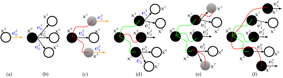
Figure 2: Graphical illustration of PINSAT. (Fig. a, b) The dummy edge $e^{d}_{0}$ from $\mathbf{x}^{0}$ is expanded to get real low-D edges $[e^{1}_{0},e^{2}_{0},e^{3}_{0}]$ but not yet evaluated with the optimizer in full-D to generate the state successor (denoted with hollow node). (c) The ePA*SE architecture in PINSAT then evaluates multiple edges in parallel (red curves). Once evaluated the outgoing nodes $\mathbf{x}^{1}\&\mathbf{x}^{3}$ are represented with dummy edges $e^{d}_{1}$ & $e^{d}_{3}$ and inserted in OPEN. This node is shown with a gray gradient to represent the underspecified full-D state for the optimization to figure out. In Fig. (d), we highlight the asynchronous execution of PINSAT. Here the dummy edges $e^{d}_{1}$ & $e^{d}_{3}$ are expanded into real edges and the $e^{2}_{0}$ is lifted to full-D by running the optimizer. Similarly, in Fig. (e), more edges are concurrently lifted to full-D. Fig. (f) denotes how the short incremental trajectory generated in Fig. (e) is reused for warm-starting the optimization and generating the trajectories from $\mathbf{x}^{S}$. This is a powerful step that dramatically increases the speed of convergence. Note that once the trajectory from $\mathbf{x}^{S}$ is generated, it replaces the low-D edge and helps drive the graph search into more informative directions.

5.2 Low Dimensional Graph Search

The low-D search runs w-eA* (Mukherjee, Aine, and Likhachev 2022a) with variations that enable its interleaving with the full-D trajectory optimization. Using w-eA* instead of wA* for the low-D search provides a systematic framework for parallelizing the expensive trajectory optimization via its parallelized variant w-ePA*SE. This is because, unlike in wA*, where the basic operation of the search loop is the expansion of a state, in w-eA*, the basic operation is the expansion of an edge.

Algorithm 2 PINSAT: Edge Expansion

1:  procedure EdgeExpandThread($i$)

2:     while $\textbf{not }terminate$ do

3:        if thread $i$ has been assigned an edge $(\mathbf{x},\mathbf{a})$ then

4:           $\textsc{Expand}\left((\mathbf{x},\mathbf{a})\right)$

5:        end if

6:     end while

7:  end procedure

8:  procedure Expand($(\mathbf{x},\mathbf{a})$)

9:     LOCK

10:     if $\mathbf{a}=\mathbf{a^{d}}$ then

11:        insert $\mathbf{x}$ in BE

12:        for $\mathbf{a}\in\mathcal{A}$ do

13:           $f\left((\mathbf{x},\mathbf{a})\right)=g(\mathbf{x})+h(\mathbf{x})$

14:           insert $(\mathbf{x},\mathbf{a})$ in OPEN with $f\left((\mathbf{x},\mathbf{a})\right)$

15:        end for

16:     else

17:        UNLOCK

18:        $\mathbf{x}^{\prime},c\left((\mathbf{x},\mathbf{a})\right)\leftarrow\textsc{GenerateSuccessor}\left((\mathbf{x},\mathbf{a})\right)$

19:        LOCK

20:        if $\mathbf{x}^{\prime}\notin\textit{CLOSED}\cup\textit{BE}$ then

21:           $\boldsymbol{\phi}(\mathbf{x}^{S}\mathbf{x}^{\prime})=\textsc{GenerateTrajectory}(\mathbf{x},\mathbf{x}^{\prime})$

22:           if $g(\mathbf{x}^{\prime})>c(\boldsymbol{\phi}(\mathbf{x}^{S}\mathbf{x}^{\prime}))$ then

23:              $g(\mathbf{x}^{\prime})=c(\boldsymbol{\phi}(\mathbf{x}^{S}\mathbf{x}^{\prime}))$

24:              $\mathbf{x}^{\prime}.parent=\mathbf{x}$

25:              $\mathbf{x}^{\prime}.traj=\boldsymbol{\phi}_{\mathbf{x}^{S}\mathbf{x}^{\prime}}$

26:              $f\left((\mathbf{x}^{\prime},\mathbf{a^{d}})\right)=g(\mathbf{x}^{\prime})+h(\mathbf{x}^{\prime})$

27:              insert/update $(\mathbf{x}^{\prime},\mathbf{a^{d}})$ in OPEN with $f\left((\mathbf{x}^{\prime},\mathbf{a^{d}})\right)$

28:           end if

29:        end if

30:        $n\_successors\_generated(\mathbf{x})+=1$

31:        if $n\_successors\_generated(\mathbf{x})=|\mathcal{A}|$ then

32:           remove $\mathbf{x}$ from BE

33:           insert $\mathbf{x}$ in CLOSED

34:        end if

35:     end if

36:     UNLOCK

37:  end procedure

w-eA*

In w-eA*, the open list (OPEN) is a priority queue of edges (not states like in wA*) that the search has generated but not expanded with the edge with the smallest priority in front of the queue. The priority of an edge is $f\left((\mathbf{x},\mathbf{a})\right)=g(\mathbf{x})+h(\mathbf{x})$. Expansion of an edge $(\mathbf{x},\mathbf{a})$ involves evaluating the edge to generate the successor $\mathbf{x}^{\prime}$ and adding/updating (but not evaluating) the edges originating from $\mathbf{x}^{\prime}$ into OPEN with the same priority of $g(\mathbf{x}^{\prime})+h(\mathbf{x}^{\prime})$. Henceforth, whenever $g(\mathbf{x}^{\prime})$ changes, the positions of all of the outgoing edges from $\mathbf{x}^{\prime}$ need to be updated in OPEN. To avoid this, ePA*SE replaces all the outgoing edges from $\mathbf{x}^{\prime}$ by a single dummy edge $(\mathbf{x}^{\prime},\mathbf{a^{d}})$, where $\mathbf{a^{d}}$ stands for a dummy action until the dummy edge is expanded. Every time $g(\mathbf{x}^{\prime})$ changes, only the dummy edge’s position has to be updated. When the dummy edge $(\mathbf{x}^{\prime},\mathbf{a^{d}})$ is expanded, it is replaced by the outgoing real edges from $\mathbf{x}^{\prime}$ in OPEN. The real edges are expanded when they are popped from OPEN by an edge expansion thread. This decoupling of the expansion of the outgoing edges from the expansion of their common parent is what enables its asynchronous parallelization.

5.3 PINSAT: Parallelized Interleaving of Search And Trajectory Optimization

The pseudocode of PINSAT is given in Alg. 1 along with a graphical illustration in Fig. 2. In graph search terminology, edge evaluation refers to computing the cost and representation of an edge that is part of the underlying graph. The optimizing step of rewiring to a better parent node, common in many search algorithms, is restricted to the edges within the graph. In contrast, a key distinction in PINSAT is that it dynamically generates edges between nodes that are not part of the low-D graph when searching for a full-D trajectory to a node. INSAT searches for this dynamic edge over the set of ancestor nodes leading to the node picked for expansion. Consequently, to make w-eA* and ePA*SE compatible with PINSAT, we search over the set of ancestor edges leading up to the edge picked for expansion (Alg. 3, line 2).

Each time the search expands a state, it removes that state from OPEN and generates the successors as per the discretization. For every low-dimensional successor, we solve a trajectory optimization problem described in the previous sections, to find a corresponding full-dimensional trajectory from the start to the successor. The trajectory optimization has access to the collision checker (implemented through callback mechanisms) and runs until convergence or collision occurrence, whichever comes first. During every iteration of the optimization, the iterates are reconstructed and checked for collision. In the case of collision, if the most recent iterate satisfies all the constraints then it is returned as a solution. If the optimized trajectory is in collision or infeasible, the algorithm enters the repair phase.

Parallelization

In w-ePA*SE, to maintain bounded sub-optimality, an edge can only be expanded if it is independent of all edges ahead of it in OPEN and the edges currently being expanded i.e. in set BE (Mukherjee, Aine, and Likhachev 2022a). However, since INSAT and therefore PINSAT are not bounded sub-optimal algorithms, the expensive independence check can be eliminated. Additionally, this increases the amount of parallelization that can be achieved. Once an edge is popped from OPEN 14, it is delegated for expansion to a spawned edge expansion thread. If all of the spawned edges are busy, a new thread is spawned as long as the total number of threads does not exceed the thread budget $N_{t}$ 31. When $N_{t}$ is higher than the number of edges available for expansion at any point in time, only a subset of available threads get spawned. This prevents performance degradation due to the operating system overhead of managing unused threads.

Algorithm 3 PINSAT: Trajectory Optimization

1:  procedure GenerateTrajectory($\mathbf{x},\mathbf{x}^{\prime}$)

2:     for $\mathbf{x}^{\prime\prime}\in\textsc{Ancestors}(\mathbf{x})\cup\mathbf{x}$ do # From $\mathbf{x}^{S}$ to $\mathbf{x}$

3:        $\boldsymbol{\phi}_{\mathbf{x}^{\prime\prime}\mathbf{x}^{\prime}}=\textsc{Optimize}(\mathbf{x}^{\prime\prime},\mathbf{x}^{\prime})$ # Eq. 15

4:        if $\boldsymbol{\phi}_{\mathbf{x}^{\prime\prime}\mathbf{x}^{\prime}}$ is collision free then

5:           $\boldsymbol{\phi}_{\mathbf{x}^{S}\mathbf{x}^{\prime}}=\textsc{WarmOptimize}(\boldsymbol{\phi}_{\mathbf{x}^{S}\mathbf{x}^{\prime\prime}},\boldsymbol{\phi}_{\mathbf{x}^{\prime\prime}\mathbf{x}^{\prime}})$ # Eq. 15

6:           return  $\boldsymbol{\phi}_{\mathbf{x}^{S}\mathbf{x}^{\prime}}$

7:        else if $\mathbf{x}^{\prime\prime}=\mathbf{x}$ then

8:           if $\boldsymbol{\phi}_{\mathbf{x}^{\prime\prime}\mathbf{x}^{\prime}}^{t_{\text{max}}}$ exists then # Solve Eq. 16

9:              $\boldsymbol{\phi}_{\mathbf{x}^{\prime\prime}\mathbf{x}^{\prime}}=\textsc{Optimize}(\mathbf{x}^{\prime\prime},\mathbf{x}^{\prime})$ # Eq. 15 with $k_{\text{min}}$

10:              $\boldsymbol{\phi}_{\mathbf{x}^{S}\mathbf{x}^{\prime}}=\textsc{WarmOptimize}(\boldsymbol{\phi}_{\mathbf{x}^{S}\mathbf{x}^{\prime\prime}},\boldsymbol{\phi}_{\mathbf{x}^{\prime\prime}\mathbf{x}^{\prime}})$ # 15

11:              return  $\boldsymbol{\phi}_{\mathbf{x}^{S}\mathbf{x}^{\prime}}$

12:           end if

13:        end if

14:        return  NULL

15:     end for

16:  end procedure

5.4 Theoretical Analysis

In this section, we will show that PINSAT is a provably complete algorithm, i.e. it finds a solution if one exists. We will begin with a few preliminaries required to prove completeness.

Definition 1.

Tunnel around Low-D Edges and Paths: For an edge $e\in\mathcal{E}$ in $G$, consider a low-D subspace corresponding to that edge called low-D tunnel of the edge $\tau_{L}(e)\subset\mathcal{X}_{L}$. The full-D tunnel for that edge is given by $\tau(e)=\tau_{L}(e)\times\mathcal{X}_{A}$. This definition can be extended to paths on the graph. Let a path between two nodes $\mathbf{x}^{\prime},\mathbf{x}^{\prime\prime}\in\mathcal{V}$ be given as $\boldsymbol{\theta}_{\mathbf{x}^{\prime}\mathbf{x}^{\prime\prime}}=\{(\mathbf{x}^{0},\mathbf{x}^{1}),(\mathbf{x}^{1},\mathbf{x}^{2}),\ldots,(\mathbf{x}^{W-1},\mathbf{x}^{W})\mid\mathbf{x}^{0}=\mathbf{x}^{\prime}\land\mathbf{x}^{W}=\mathbf{x}^{\prime\prime}\land(\mathbf{x}^{w-1},\mathbf{x}^{w})\in\mathcal{E},1\leq w\leq W\}$. Then a tunnel around $\boldsymbol{\theta}_{\mathbf{x}^{\prime}\mathbf{x}^{\prime\prime}}$ is given as $\tau(\boldsymbol{\theta}_{\mathbf{x}^{\prime}\mathbf{x}^{\prime\prime}})=\cup_{e\in\boldsymbol{\theta}_{\mathbf{x}^{\prime}\mathbf{x}^{\prime\prime}}}\tau(e)$.

Assumption 1.

We assume that there exists at least a path on the low-D graph $G$ form $\mathbf{x}^{S}$ to $\mathbf{x}^{G}$ such that its full-D tunnel contains $\boldsymbol{\phi}_{\textbf{x}^{S}\textbf{x}^{G}}$, i.e. $\exists\boldsymbol{\theta}_{\textbf{x}^{S}\textbf{x}^{G}}\in G\mid\exists\boldsymbol{\phi}_{\textbf{x}^{S}\textbf{x}^{G}}\in\tau(\boldsymbol{\theta}_{\textbf{x}^{S}\textbf{x}^{G}})$.

Assumption 2.

$\forall e\in\mathcal{E}$, $\tau(e)$ is convex.

Minimum Order of B-spline:

The minimum order $k_{\text{min}}$ of the B-spline $\boldsymbol{\phi}_{k_{\text{min}}}(t)$ with control points $\textbf{P}=\{\textbf{p}_{0},\ldots,\textbf{p}_{m}\}$ that is (i) guaranteed to lie entirely within the full-D tunnel of any edge $e=(\mathbf{x}^{\prime},\mathbf{x}^{\prime\prime})\in\mathcal{E}$ and (ii) satisfy constraints on its derivatives (similar to Eq. 15d) can be found by solving the simple optimization below

$$k_{\text{min}}=\ \ \max_{e\in\mathcal{E}}\ \min_{k_{e}}\ \ k_{e}$$ (17a)

s.t. $$\textbf{p}_{0}=\mathbf{x}^{\prime},\textbf{p}_{m}=\textbf{x}^{\prime\prime}$$ (17b)

$$\boldsymbol{\phi}_{k_{\text{min}}}(t)\in\tau_{L}(e);0\leq t\leq t_{\text{min}}$$ (17c)

$$|\textbf{p}_{0}^{(j)}|,|\textbf{p}_{k_{e}-j}^{(j)}|=t_{\text{min}}^{j}\boldsymbol{\phi}^{(j)}_{\text{lim}}$$ (17d)

$$|\textbf{p}_{1}^{(j)}|,\ldots,|\textbf{p}_{k_{e}-j-1}^{(j)}|\leq t_{\text{min}}^{j}\boldsymbol{\phi}^{(j)}_{\text{lim}}$$ (17e)

The tunnel constraints in Eq 17c are transcribed into constraints on the control points similar to how corridor constraints are represented in (Rousseau et al. 2019). In this work, the outer maximization is carried over actions set $\mathcal{A}$, which is typically a significantly smaller set than $\mathcal{E}$. This can be done if the edges in the graph can be grouped as a finite number of action primitives sharing the same tunnel representation. Note that the inner optimization in the above formulation is a linear program and is guaranteed to have at least one solution as long as the feasible region of the decision variable is nonempty and bounded.

Remark 4.

The feasible region depends on the limits of the system $\boldsymbol{\phi}^{(j)}_{\text{lim}}$ and the choice of the tunnel $\tau$ which is domain-specific. However, in most cases, a straightforward design of the tunnel (Rousseau et al. 2019) can ensure a nonempty feasible region and a reasonably low $k_{\text{min}}$.

Consider an edge $e=(\mathbf{x}^{\prime},\mathbf{x}^{\prime\prime})\in\mathcal{E}$.

Lemma 1.

If $\tau(e)$ is convex, then a $\boldsymbol{\phi}_{\mathbf{x}^{\prime}\mathbf{x}^{\prime\prime}}^{\sim}(t)\in\tau(e),\forall t\in[0,t_{\text{max}}]$ that solves Eq. 16 to global optimality can be found.

Proof.

Setting $\mathcal{X}^{\text{free}}=\tau(e)$ make Eq. 16d a convex domain constraint on the decision variables and Eq. 16 a convex program. Assuming $t_{\text{max}}$ is large enough, we know that a convex optimization can be solved to global optimality. ∎

Let $\boldsymbol{\hat{\phi}}_{\mathbf{x}^{\prime}\mathbf{x}^{\prime\prime}}\in\mathcal{C}^{\gamma}(\mathbb{R})$. $\boldsymbol{\hat{\phi}}_{\mathbf{x}^{\prime}\mathbf{x}^{\prime\prime}}$ need not satisfy $\boldsymbol{\phi}_{\text{lim}}^{(j)},j\leq\gamma$.

Lemma 2.

If $\boldsymbol{\hat{\phi}}_{\mathbf{x}^{\prime}\mathbf{x}^{\prime\prime}}\in\tau_{L}(e)$, then there exists a $k_{\text{min}}$-th order $\boldsymbol{\phi}_{\mathbf{x}^{\prime}\mathbf{x}^{\prime\prime}}^{*}\in\tau(e)$ that satisfies Eq. 15.

Proof.

It directly follows from the constraint satisfaction for finding $k_{\text{min}}$ in Eq. 17. This $k_{\text{min}}$ can be used to choose the B-spline basis for optimizing Eq. 15 simultaneously over path length and time to find $\boldsymbol{\phi}_{\mathbf{x}^{\prime}\mathbf{x}^{\prime\prime}}^{*}\in\tau(e)$. ∎

In other words, Lemma. 2 states that if there is a trajectory that is (i) $\mathcal{C}^{j}$-continuous, (ii) satisfies the low-D boundary conditions of an edge $e\in\mathcal{E}$ and, (iii) is contained entirely within the low-D tunnel of the edge $\tau_{L}(e)$, then we can use $k_{\text{min}}$-th order basis functions to construct a trajectory that satisfies full-D $j$-th derivative boundary conditions and lies entirely within the full-D tunnel of the edge $\tau(e)$. We note that Lemma. 2 is a critical building block towards developing PINSAT’s guarantee on completeness.

Theorem 1.

Completeness of PINSAT: If Assumption 1 holds, then PINSAT with $k_{\text{min}}$-th order B-spline optimization is guaranteed to find a $\boldsymbol{\phi}_{\mathbf{x}^{S}\mathbf{x}^{G}}$ that satisfies Eq. 1.

6 Evaluation

	pBiRRT +TrajOpt				w-ePA*SE +TrajOpt				INSAT	PINSAT
Threads	5	10	50	120	5	10	50	120	1	5	10	50	120
Success rate ($\%$)	1	1	3	2	0	0	6	2	58	72	81	90	90
Time ($\mathrm{s}$)	0.03$\pm$0.02	0.021$\pm$0.02	0.02$\pm$0.01	0.02$\pm$0.01	0.38$\pm$0.35	0.30$\pm$0.31	0.28$\pm$0.32	0.27$\pm$0.30	2.02$\pm$2.01	0.70$\pm$0.91	0.43$\pm$0.6	0.43$\pm$0.31	0.99$\pm$0.72
Cost	5.18$\pm$2.89	4.88$\pm$2.75	4.55$\pm$2.48	4.25$\pm$2.24	9.19$\pm$4.23	8.71$\pm$4.00	8.34$\pm$3.89	8.23$\pm$3.76	1.55$\pm$2.68	0.51$\pm$1.11	1.10$\pm$2.06	1.47$\pm$2.54	1.57$\pm$2.62

Table 1: Mean and standard deviation of planning time and cost for PINSAT and the baselines for different thread budgets.

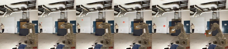
Figure 3: PINSAT used accelerate preprocessing of a motion library for rapid lookup. Here an ABB arm with a shield attached to its end-effector executes a motion generated by PINSAT to block a ball thrown at it.

We evaluate PINSAT in a kinodynamic manipulation planning for an ABB IRB 1600 industrial robot shown in Fig 1. The red horizontal and vertical bars are obstacles and divide the region around the robot into eight quadrants, four below the horizontal bars and four above. We randomly sample 500 hard start and goal configurations. We ensure that the end effector corresponding to one of those configurations is above the horizontal bars and the other is underneath. We also ensure that the end effector for the start and goal configurations are not sampled in the region enclosed by the same two adjacent vertical bars. Our samples are deliberately far apart in the manipulator’s C-space and require long spatial and temporal plans to connect them. The motivation for sampling start-goal pairs in this manner is to subject the planner to stress tests under severe constraints on the duration of the trajectory. All the experiments are run on an AMD Ryzen Threadripper Pro with 128 threads.

For our experiments, we use a backward breadth-first search (BFS) from the goal state in the task space of the manipulator as our heuristic. The action space $\mathcal{A}$ is made of small unit joint movements. For every joint, we had a $4\deg$ and $7\deg$ primitive in each direction subject to the joint limits. In addition to this, during every state expansion, we also check if the goal state is the line of sight to consider the goal as a potential successor. The velocity limits of the arm were inflated 10x the values specified in the datasheet for simulation. We used $50m/s^{2}$ and $200m/s^{3}$ as the acceleration and jerk limits. The maximum duration of trajectory was limited to 0.6s. The reason for inflating the velocity limits is to allow the bare minimum time to navigate the obstacles and reach from start to goal.

Table 1 shows success rate and planning time statistics for INSAT and PINSAT for different thread budgets. The planning time statistics were only computed over the problems successfully solved by both algorithms for a given thread budget. We also implemented a parallelized version of RRTConnect (pBiRRT) as a baseline. The kinematic plan generated by pBiRRT was then post-processed by the same B-spline optimization used in PINSAT to compute the final kinodynamic plan. As the optimization has a constraint on the maximum execution duration of the trajectory, adding all the waypoints from the path at once will result in an over-constrained system of equations for which a solution may not exist. To circumvent this, we iteratively add the waypoint constraint starting from the minimum containing just the start and the goal state. Though pBiRRT had a 100% success rate in computing the spatial trajectory, the results after post-processing with the optimizer were abysmal. PINSAT achieves a significantly higher success rate than INSAT for all thread budgets greater than 1. Specifically, it achieves a 5x improvement in mean planning time, a 7x improvement in median planning time, and a 1.8x improvement in success rate for $N_{t}$ = 60. Even with a single thread, PINSAT achieves lower planning times than INSAT. This is because of the decoupling of edge evaluations from state expansions in ePA*SE.

7 Conclusion

We presented PINSAT, which parallelizes the interleaving of search and trajectory optimization using the ideas of ePA*SE (Mukherjee, Aine, and Likhachev 2022a). In a kinodynamic manipulation planning domain, PINSAT achieved significantly higher success rates than INSAT (Natarajan, Choset, and Likhachev 2021; Natarajan et al. 2023) and a drastic reduction in planning time.

References

- Aine et al. (2016) Aine, S.; Swaminathan, S.; Narayanan, V.; Hwang, V.; and Likhachev, M. 2016. Multi-heuristic A*. The International Journal of Robotics Research, 35(1-3): 224–243.
- Alwala and Mukadam (2021) Alwala, K. V.; and Mukadam, M. 2021. Joint sampling and trajectory optimization over graphs for online motion planning. In 2021 IEEE/RSJ International Conference on Intelligent Robots and Systems (IROS), 4700–4707. IEEE.
- Betts (2010) Betts, J. T. 2010. Practical methods for optimal control and estimation using nonlinear programming. SIAM.
- Choudhury et al. (2016) Choudhury, S.; Gammell, J. D.; Barfoot, T. D.; Srinivasa, S. S.; and Scherer, S. 2016. Regionally accelerated batch informed trees (rabit*): A framework to integrate local information into optimal path planning. In 2016 IEEE International Conference on Robotics and Automation (ICRA), 4207–4214. IEEE.
- Chow, Chang, and Hollinger (2023) Chow, S.; Chang, D.; and Hollinger, G. A. 2023. Parallelized Control-Aware Motion Planning With Learned Controller Proxies. IEEE Robotics and Automation Letters, 8(4): 2237–2244.
- De Boor (1978) De Boor, C. 1978. A practical guide to splines, volume 27. springer-verlag New York.
- Devaurs, Siméon, and Cortés (2011) Devaurs, D.; Siméon, T.; and Cortés, J. 2011. Parallelizing RRT on distributed-memory architectures. In 2011 IEEE International Conference on Robotics and Automation, 2261–2266.
- Evett et al. (1995) Evett, M.; Hendler, J.; Mahanti, A.; and Nau, D. 1995. PRA*: Massively parallel heuristic search. Journal of Parallel and Distributed Computing, 25(2): 133–143.
- Gammell, Srinivasa, and Barfoot (2015) Gammell, J. D.; Srinivasa, S. S.; and Barfoot, T. D. 2015. Batch informed trees (BIT*): Sampling-based optimal planning via the heuristically guided search of implicit random geometric graphs. In 2015 IEEE international conference on robotics and automation (ICRA), 3067–3074. IEEE.
- Hart, Nilsson, and Raphael (1968) Hart, P. E.; Nilsson, N. J.; and Raphael, B. 1968. A formal basis for the heuristic determination of minimum cost paths. IEEE transactions on Systems Science and Cybernetics, 4(2): 100–107.
- Hauser and Zhou (2016) Hauser, K.; and Zhou, Y. 2016. Asymptotically optimal planning by feasible kinodynamic planning in a state–cost space. IEEE Transactions on Robotics, 32(6): 1431–1443.
- He et al. (2021) He, X.; Yao, Y.; Chen, Z.; Sun, J.; and Chen, H. 2021. Efficient parallel A* search on multi-GPU system. Future Generation Computer Systems, 123: 35–47.
- Ichnowski and Alterovitz (2012) Ichnowski, J.; and Alterovitz, R. 2012. Parallel sampling-based motion planning with superlinear speedup. In IROS, 1206–1212.
- Irani and Shih (1986) Irani, K.; and Shih, Y.-f. 1986. Parallel A* and AO* algorithms- An optimality criterion and performance evaluation. In 1986 International Conference on Parallel Processing, University Park, PA, 274–277.
- Jacobs et al. (2012) Jacobs, S. A.; Manavi, K.; Burgos, J.; Denny, J.; Thomas, S.; and Amato, N. M. 2012. A scalable method for parallelizing sampling-based motion planning algorithms. In 2012 IEEE International Conference on Robotics and Automation, 2529–2536.
- Jacobs et al. (2013) Jacobs, S. A.; Stradford, N.; Rodriguez, C.; Thomas, S.; and Amato, N. M. 2013. A scalable distributed RRT for motion planning. In 2013 IEEE International Conference on Robotics and Automation, 5088–5095.
- Kamat et al. (2022) Kamat, J.; Ortiz-Haro, J.; Toussaint, M.; Pokorny, F. T.; and Orthey, A. 2022. Bitkomo: Combining sampling and optimization for fast convergence in optimal motion planning. In 2022 IEEE/RSJ International Conference on Intelligent Robots and Systems (IROS), 4492–4497. IEEE.
- Kavraki et al. (1996) Kavraki, L. E.; Svestka, P.; Latombe, J.-C.; and Overmars, M. H. 1996. Probabilistic roadmaps for path planning in high-dimensional configuration spaces. IEEE tran. on Robot. Autom., 12(4): 566–580.
- Kicki et al. (2023) Kicki, P.; Liu, P.; Tateo, D.; Bou-Ammar, H.; Walas, K.; Skrzypczyński, P.; and Peters, J. 2023. Fast Kinodynamic Planning on the Constraint Manifold with Deep Neural Networks. arXiv preprint arXiv:2301.04330.
- Kunz and Stilman (2015) Kunz, T.; and Stilman, M. 2015. Kinodynamic RRTs with fixed time step and best-input extension are not probabilistically complete. In Algorithmic Foundations of Robotics XI: Selected Contributions of the Eleventh International Workshop on the Algorithmic Foundations of Robotics, 233–244. Springer.
- Kusnur et al. (2021) Kusnur, T.; Mukherjee, S.; Saxena, D. M.; Fukami, T.; Koyama, T.; Salzman, O.; and Likhachev, M. 2021. A planning framework for persistent, multi-uav coverage with global deconfliction. In Field and Service Robotics, 459–474. Springer.
- Lau, Sprunk, and Burgard (2009) Lau, B.; Sprunk, C.; and Burgard, W. 2009. Kinodynamic motion planning for mobile robots using splines. In 2009 IEEE/RSJ International Conference on Intelligent Robots and Systems, 2427–2433. IEEE.
- LaValle and Kuffner Jr (2001) LaValle, S. M.; and Kuffner Jr, J. J. 2001. Randomized kinodynamic planning. Int. J. Robot. Research, 20(5): 378–400.
- LaValle et al. (1998) LaValle, S. M.; et al. 1998. Rapidly-exploring random trees: A new tool for path planning.
- Li et al. (2021) Li, L.; Miao, Y.; Qureshi, A. H.; and Yip, M. C. 2021. Mpc-mpnet: Model-predictive motion planning networks for fast, near-optimal planning under kinodynamic constraints. IEEE Robotics and Automation Letters, 6(3): 4496–4503.
- Liang et al. (2021) Liang, J.; Sharma, M.; LaGrassa, A.; Vats, S.; Saxena, S.; and Kroemer, O. 2021. Search-Based Task Planning with Learned Skill Effect Models for Lifelong Robotic Manipulation. arXiv preprint arXiv:2109.08771.
- Likhachev and Ferguson (2009) Likhachev, M.; and Ferguson, D. 2009. Planning long dynamically feasible maneuvers for autonomous vehicles. The International Journal of Robotics Research, 28(8): 933–945.
- Littlefield and Bekris (2018) Littlefield, Z.; and Bekris, K. E. 2018. Efficient and asymptotically optimal kinodynamic motion planning via dominance-informed regions. In 2018 IEEE/RSJ International Conference on Intelligent Robots and Systems (IROS), 1–9. IEEE.
- Liu, Lai, and Wu (2013) Liu, H.; Lai, X.; and Wu, W. 2013. Time-optimal and jerk-continuous trajectory planning for robot manipulators with kinematic constraints. Robotics and Computer-Integrated Manufacturing, 29(2): 309–317.
- Mukherjee, Aine, and Likhachev (2022a) Mukherjee, S.; Aine, S.; and Likhachev, M. 2022a. ePA*SE: Edge-Based Parallel A* for Slow Evaluations. In International Symposium on Combinatorial Search, volume 15, 136–144. AAAI Press.
- Mukherjee, Aine, and Likhachev (2022b) Mukherjee, S.; Aine, S.; and Likhachev, M. 2022b. MPLP: Massively Parallelized Lazy Planning. IEEE Robotics and Automation Letters, 7(3): 6067–6074.
- Mukherjee et al. (2021) Mukherjee, S.; Paxton, C.; Mousavian, A.; Fishman, A.; Likhachev, M.; and Fox, D. 2021. Reactive long horizon task execution via visual skill and precondition models. In 2021 IEEE/RSJ International Conference on Intelligent Robots and Systems (IROS), 5717–5724. IEEE.
- Natarajan, Choset, and Likhachev (2021) Natarajan, R.; Choset, H.; and Likhachev, M. 2021. Interleaving graph search and trajectory optimization for aggressive quadrotor flight. IEEE Robotics and Automation Letters, 6(3): 5357–5364.
- Natarajan et al. (2023) Natarajan, R.; Johnston, G. L.; Simaan, N.; Likhachev, M.; and Choset, H. 2023. Torque-limited manipulation planning through contact by interleaving graph search and trajectory optimization. In 2023 IEEE International Conference on Robotics and Automation (ICRA), 8148–8154. IEEE.
- Ortiz-Haro et al. (2023) Ortiz-Haro, J.; Hoenig, W.; Hartmann, V. N.; and Toussaint, M. 2023. iDb-A*: Iterative Search and Optimization for Optimal Kinodynamic Motion Planning. arXiv preprint arXiv:2311.03553.
- Phillips, Likhachev, and Koenig (2014) Phillips, M.; Likhachev, M.; and Koenig, S. 2014. PA* SE: Parallel A* for slow expansions. In Twenty-Fourth International Conference on Automated Planning and Scheduling.
- Piegl and Tiller (1996) Piegl, L.; and Tiller, W. 1996. The NURBS book. Springer Science & Business Media.
- Pohl (1970) Pohl, I. 1970. Heuristic search viewed as path finding in a graph. Artificial intelligence, 1(3-4): 193–204.
- Rousseau et al. (2019) Rousseau, G.; Maniu, C. S.; Tebbani, S.; Babel, M.; and Martin, N. 2019. Minimum-time B-spline trajectories with corridor constraints. Application to cinematographic quadrotor flight plans. Control Engineering Practice, 89: 190–203.
- Sakcak et al. (2019) Sakcak, B.; Bascetta, L.; Ferretti, G.; and Prandini, M. 2019. Sampling-based optimal kinodynamic planning with motion primitives. Autonomous Robots, 43(7): 1715–1732.
- Schulman et al. (2014) Schulman, J.; Duan, Y.; Ho, J.; Lee, A.; Awwal, I.; Bradlow, H.; Pan, J.; Patil, S.; Goldberg, K.; and Abbeel, P. 2014. Motion planning with sequential convex optimization and convex collision checking. The International Journal of Robotics Research, 33(9): 1251–1270.
- Tassa, Mansard, and Todorov (2014) Tassa, Y.; Mansard, N.; and Todorov, E. 2014. Control-limited differential dynamic programming. In 2014 IEEE International Conference on Robotics and Automation (ICRA), 1168–1175. IEEE.
- Toussaint (2017) Toussaint, M. 2017. A tutorial on Newton methods for constrained trajectory optimization and relations to SLAM, Gaussian Process smoothing, optimal control, and probabilistic inference. Geometric and numerical foundations of movements, 361–392.
- Zhou and Zeng (2015) Zhou, Y.; and Zeng, J. 2015. Massively parallel A* search on a GPU. In Proceedings of the AAAI Conference on Artificial Intelligence.