Topological charge pumping in dimerized Kitaev chains

Abstract

We investigated the topological pumping charge of a dimerized Kitaev chain with spatially modulated chemical potential, which hosts nodal loops in parameter space and violates particle number conservation. In the simplest case, with alternatively assigned hopping and pairing terms, we show that the model can be mapped into the Rice-Mele model by a partial particle-hole transformation and subsequently supports topological charge pumping as a demonstration of the Chern number for the ground state. Beyond this special case, analytic analysis shows that the nodal loops are conic curves. Numerical simulation of a finite-size chain indicates that the pumping charge is zero for a quasiadiabatic loop within the nodal loop and is $\pm 1$ for a quasiadiabatic passage enclosing the nodal loop. Our findings unveil a hidden topology in a class of Kitaev chains.

Introduction

Thouless pumping Thouless1983Quan has received much attention over a long period of time. It is the quantum version of matter pumping by a mechanical device in our everyday life. The intriguing features are that (i) the total probability of the transferred particles is precisely quantized for a cyclic adiabatic passage without a bias voltage and (ii) a nonzero pumping charge for the ground state is shown to relate a degenerate point and then acts as a topological invariant XiaoDi .

Recent enhanced quantum manipulation techniques allowing precise control of the time-dependent periodic potential have made experimental realization of quantum pumping possible. Electron pumping experiments have been performed in various semiconductor-based nanoscale devices Switkes1999a ; Blumenthal2007 ; kaestner2008single . More recently, the topological charge pump was realized in optical superlattices based on ultracold atom technology nakajima2016topological ; lohse2016thouless ; lu2016geometrical , and it was also extensively studied in theory chiang1998quantum ; qian2011quantum ; wang2013topological ; matsuda2014topological ; mei2014topological ; wei2015anomalous ; yang2018continuously ; Matsuda2022 ; zhang2020top . To date, both experimental and theoretical studies have focused mainly on systems that involve the conversion of particles, such as 1D or 2D topological insulators.

In this work, we studied the topological pumping charge of a dimerized Kitaev chain model with spatially modulated chemical potential. In general, the topological pumping charge in a one-dimensional Kitaev model refers to the corresponding Majorana lattice rather than the transport of spinless fermions XiaoDi ; WR1 ; WR2 . Technically, the origin of this topological feature is the degenerate point. In contrast, the present dimerized Kitaev model hosts nodal loops in parameter space, and the pumping charge is obtained directly from the ground state of the model, which does not support particle number conservation. The main motivation of this work arises from the simplest case in which the hopping and pairing terms are completely assigned to different dimers alternatively. We show that this model can be mapped into a Rice-Mele (RM) model Rice by a partial particle-hole transformation under certain constraints. Then, the ground state of such a Kitaev model supports the topological charge pumping as a demonstration of the Chern number because the current operator is invariant under the transformation. Beyond this special case, analytic analysis has shown that the degenerate points become nodal loops. Numerical simulation of a finite-size chain indicates that the pumping charge is zero for a quasiadiabatic loop within the nodal loop and $\pm 1$ for the passage loop enclosing the nodal loop. Our findings unveil a hidden topology in a class of Kitaev chains.

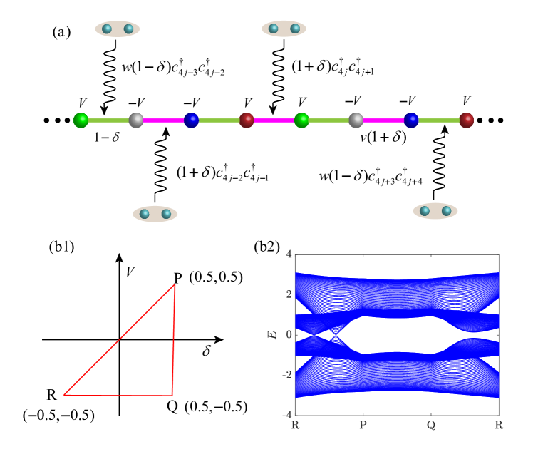
Figure 1: (a) A schematic diagram of the Hamiltonian in Eq. (1). A unit cell is composed of four sites with modulated chemical potential. The strengths of the hopping terms and pairing terms are stagger. $1-\delta$ and $v\left(1+\delta\right)$ are the strengths of the hopping terms, and $w\left(1-\delta\right)$ and $1+\delta$ are the strengths of pair creation (annihilation). (b1) shows a triangular loop on the $\delta-V$ plane, and (b2) shows the corresponding energy spectra along the loop. The spectra are symmetrical with respect to zero, and there are two degenerate points because the loop has two crossing points with the degenerate line of the energy spectra. The parameters are $N=50,w=0.6,$ and $v=-0.3$.

The rest of the paper is organized as follows. We begin Sec. I by introducing the Hamiltonian and its symmetry. We also analytically deduce the equations of nodal lines in parameter space. In Sec. II we demonstrate that the model under some constraints can be mapped into the Rice-Mele model via a partial particle-hole transformation, which inspires us to investigate the pumping charge of this model. In Sec. III, we numerically calculate the pumping charges of the ground state for different quasiadiabatic passages in parameter space. The results indicate that the pumping charge can be treated as a topological invariant to characterize the topology of the model. Finally, we draw conclusions in Sec. IV. Some detailed derivations are given in the Appendix.

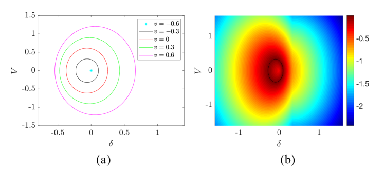
Figure 2: (a) Several representative nodal lines derived from Eq. (12) on the $\delta-V$ plane for fixed $w$ and different $v$. (b) Color contour plots of the numerical results of one of the energy bands with the wavevector $k=0$. The black loop is the nodal line from (a) with $v=-0.3$ and this indicates that the degenerate line on the $\delta-V$ plane is a closed loop, which accords with that in (a). The other parameters are $N=50$ and $w=0.6$.

I Model and nodal ellipses

The Kitaev chain model describes a spin-polarized $p$-wave superconductor in a one-dimensional system and has received much attention since its simple form also includes a rich phase diagram. This system has a topological phase, realizing Majorana zero modes at the ends of the chain Kitaev . On the other hand, it is the fermionized version of the well-known one-dimensional transverse-field Ising model Pfeuty , which is one of the simplest solvable models that exhibit quantum criticality and phase transition with spontaneous symmetry breaking SachdevBook . Several studies have been conducted with a focus on long-range Kitaev chains, in which the superconducting pairing term decays with distance as a power law TPCHOY ; AGG ; DV1 ; DV2 ; OV ; LL ; UB .

In this work, we investigate the topological features of the Kitaev chain from an alternative perspective, referred to as the hidden topology. Such a feature does not emerge in the usual Kitaev chain considered in the literature. Considering a dimerized one-dimensional Kitaev model, the Hamiltonian contains two parts

$$H=H_{1}+H_{2},$$ (1)

with

$$H_{1} = \sum_{l=1}^{2N}\left[\left(1-\delta\right)c_{2l-1}^{{\dagger}}c_{2l}+\left(1+\delta\right)c_{2l}^{{\dagger}}c_{2l+1}^{{\dagger}}\right]+\mathrm{h.c.}$$ (2)

$$+V\sum_{l=1}^{2N}\left(-1\right)^{l+1}\left(c_{2l-1}^{{\dagger}}c_{2l-1}-c_{2l}^{{\dagger}}c_{2l}\right),$$

and

$$H_{2}=\sum_{l=1}^{2N}\left[\left(1-\delta\right)wc_{2l-1}^{{\dagger}}c_{2l}^{{\dagger}}+\left(1+\delta\right)vc_{2l}^{{\dagger}}c_{2l+1}\right]+\mathrm{h.c.}.$$ (3)

The dimerized Kitaev model is schematically illustrated in Fig. 1 (a). This seems to be somewhat complicated, and the purpose of this separation is to provide a better presentation for the following discussions. Here, $c_{j}$ denotes the fermion annihilation operator at site $j$. $\left(1\pm\delta\right)$ are the hopping amplitudes and the strength of the pairing operator between neighboring sites with dimerized factors $1$, $v$, and $w$, and the real number $V$ is the chemical potential. When the periodic boundary is taken, we define $c_{4N+j}=c_{j}$.

For arbitrary parameters, the unit cell includes four sites. Then, the Hamiltonian $H$ can be written in block diagonal form

$$H=\sum_{\pi>k>0}\Psi_{k}h_{k}\Psi_{k}^{{\dagger}}=\sum_{\pi>k>0}\Psi_{k}\left(\begin{array}[]{cc}A&-B\\ B&-A\end{array}\right)\Psi_{k}^{{\dagger}},$$ (4)

by introducing Fourier transformation

$$\left(\begin{array}[]{c}c_{4j-3}\\ c_{4j-2}\\ c_{4j-1}\\ c_{4j}\end{array}\right)=\frac{e^{ikj}}{\sqrt{N}}\sum\limits_{k}\left(\begin{array}[]{c}\alpha_{k}\\ \gamma_{k}\\ \beta_{k}\\ \eta_{k}\end{array}\right),$$ (5)

with $k=2\pi m/N$, $m=1,2,\cdots N$. Here, the operator vector is defined as

$$\Psi_{k}=\left(\begin{array}[]{cccccccc}\alpha_{k}^{{\dagger}}&\gamma_{k}^{{\dagger}}&\beta_{k}^{{\dagger}}&\eta_{k}^{{\dagger}}&\alpha_{-k}&\gamma_{-k}&\beta_{-k}&\eta_{-k}\end{array}\right),$$ (6)

and the two $4\times 4$ matrices $A$ and $B$ are

$$A=\left(\begin{array}[]{cccc}V&1-\delta&0&v\Gamma_{-k}\\ 1-\delta&-V&v\Gamma_{0}&0\\ 0&v\Gamma_{0}&-V&1-\delta\\ v\Gamma_{k}&0&1-\delta&V\end{array}\right),$$ (7)

and

$$B=w\left(\begin{array}[]{cccc}0&\delta-1&0&\Gamma_{-k}/w\\ 1-\delta&0&-\Gamma_{0}/w&0\\ 0&\Gamma_{0}/w&0&\delta-1\\ -\Gamma_{k}/w&0&1-\delta&0\end{array}\right),$$ (8)

where the $k$-dependent factor $\Gamma_{k}=\left(1+\delta\right)e^{ik}$. The symmetry of the matrix $h_{k}$ contains the core information of the system, which allows us to obtain the conclusion without solving the $8\times 8$ matrix $h_{k}$ explicitly.

Introducing the $8\times 8$ matrix

$$P=\left(\begin{array}[]{cc}0&I_{2}\\ I_{2}&0\end{array}\right),I_{2}=\left(\begin{array}[]{cc}1&0\\ 0&1\end{array}\right),$$ (9)

we readily have

$$P\left(\begin{array}[]{cc}A&-B\\ B&-A\end{array}\right)P^{-1}=-\left(\begin{array}[]{cc}A&-B\\ B&-A\end{array}\right),$$ (10)

which ensures that the spectrum $\varepsilon_{k}$ of $h_{k}$ is symmetric with respect to the zero-energy point. This can be demonstrated by numerical simulations for finite-size chains. The spectra of the system with representative parameters are plotted in Fig. 1 (b2). Furthermore, $\left|\varepsilon_{k}\right|$ can be obtained directly from the diagonalization of the $4\times 4$ matrix $\left(A+B\right)\left(A-B\right)$ (details are shown in the Appendix).

In the following, we focus on the degeneracy points of $\varepsilon_{k}$ in the parameter space. The derivations in the Appendix show that the band degenerate points always lay in the subspace with $k=0$ or $\pi$, i.e., the degenerate zero-energy points (nodal line) can be determined by

$$\varepsilon_{0}\varepsilon_{\pi}=0.$$ (11)

Then, the corresponding nodal lines obey the equations

$$\left(\frac{\delta+c_{1}}{a_{1}}\right)^{2}+\left(\frac{V}{b_{1}}\right)^{2}=1,$$ (12)

and

$$\left(\frac{\delta+c_{2}}{a_{2}}\right)^{2}-\left(\frac{V}{b_{2}}\right)^{2}=1,$$ (13)

which are obviously an ellipse and a hyperbola, respectively. Here, the shapes of two conic curves are determined by the system parameters

$$a_{1} = \frac{2\left(w+v\right)}{4-\left(w-v\right)^{2}},a_{2}=\frac{2}{w+v},$$ (14)

$$b_{1} = \frac{2\left(w+v\right)}{\sqrt{4-\left(w-v\right)^{2}}},b_{2}=2,$$ (15)

$$c_{1} = \frac{w^{2}-v^{2}}{4-\left(w-v\right)^{2}},c_{2}=\frac{v-w}{v+w}.$$ (16)

We note that when taking $w+v\rightarrow 0$ (see also the exact solution for $w+v=0$ in the following section), the first equation reduces to a point $\left(\delta,V\right)=\left(0,0\right)$ if $\left|w\right|<1$. In this work, we focus on the nodal line around the point $\left(\delta,V\right)=\left(0,0\right)$. The corresponding nodal lines and energy band edges are plotted in Fig. 2 (a) and (b). In the following, we will investigate the topological features related to the nodal lines. This study differs from all the previous work on nodal lines, which are lines in 3D space, while the present study appears only in 2D space.

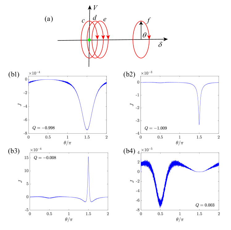
Figure 3: The adiabatic current in Eq. (30) and pumping charge in Eq. (31) of the ground state of the Hamiltonian with a single degenerate point for different passages. (a) The green solid dot is the degenerate point $\left(\delta,V\right)=\left(0,0\right)$ and the red lines represent different adiabatic loops. The equations are $\delta=\sin\left(\omega t\right)+\delta_{0}$, $V=3\cos\left(\omega t\right)$ and $\theta=\omega t$; for $c,d,e,$ and $f$, the parameters $\delta_{0}$ are 0, 0.9, 1.1, and 2, respectively; and (b1), (b2), (b3) and (b4) show the corresponding numerical results of the adiabatic current and pumping charge. The time interval is $t_{l}-t_{l-1}=0.0628$, and the other parameters are $w=0.6,v=-0.6$, $\omega=0.001$, and $N=50$. This implies that if the adiabatic loop encircles the degenerate point, the pumping charge is nearly -1; otherwise, the pumping charge is nearly 0.

II Equivanlent RM model

In this section, we start with a Kitaev model that connects to a well-known model possessing topological features. We consider the Hamiltonian $H$ with $v=-w$, at which the Hamiltonian becomes a simplified form

$$h_{k}=h_{1}^{k}+h_{2}^{k}=\sum_{l=1,2}\left(\begin{array}[]{cc}A_{l}&-B_{l}\\ B_{l}&-A_{l}\end{array}\right),$$ (17)

and obey the commutative relations

$$\left[h_{1}^{k},h_{2}^{k}\right]=\left[H_{1},H_{2}\right]=0.$$ (18)

The relations can be checked by a straightforward derivation for the following explicit forms of four matrices. Here, two $k$-independent $4\times 4$ matrices are

$$A_{1}=\left(\begin{array}[]{cccc}V&1-\delta&0&0\\ 1-\delta&-V&0&0\\ 0&0&-V&1-\delta\\ 0&0&1-\delta&V\end{array}\right),$$ (19)

and

$$B_{2}=w\left(1-\delta\right)\left(\begin{array}[]{cccc}0&-1&0&0\\ 1&0&0&0\\ 0&0&0&-1\\ 0&0&1&0\end{array}\right),$$ (20)

while the other two $k$-dependent ones are

$$B_{1}=\left(1+\delta\right)\left(\begin{array}[]{cccc}0&0&0&e^{-ik}\\ 0&0&-1&0\\ 0&1&0&0\\ -e^{ik}&0&0&0\end{array}\right),$$ (21)

and

$$A_{2}=-\left(1+\delta\right)w\left(\begin{array}[]{cccc}0&0&0&e^{-ik}\\ 0&0&1&0\\ 0&1&0&0\\ e^{ik}&0&0&0\end{array}\right).$$ (22)

Obviously, $H$ and $H_{1}$ have common eigenstates. Importantly, the derivation in the Appendix shows that $H$ and $H_{1}$ have the same ground state within the region $\left|w\right|<1$. This means that one can focus on the investigation and analysis of $H_{1}$ only. Notably, we will show that $H_{1}$ has a connection to a RM model.

Taking a partial particle-hole transformation

$$\left(\begin{array}[]{c}c_{4j-3}\\ c_{4j-2}\\ c_{4j-1}\\ c_{4j}\end{array}\right)\longrightarrow\left(\begin{array}[]{c}c_{4j-3}^{{\dagger}}\\ c_{4j-2}^{{\dagger}}\\ c_{4j-1}\\ -c_{4j}\end{array}\right),$$ (23)

with $j\in\left[1,N\right]$, $H_{1}$ becomes a RM model Rice

$$H_{\mathrm{RM}} = -\sum_{l=1}^{2N}\left[\left(1-\delta\right)c_{2l-1}^{{\dagger}}c_{2l}+\left(1+\delta\right)c_{2l}^{{\dagger}}c_{2l+1}\right]+\mathrm{h.c.}$$ (24)

$$+V\sum_{l=1}^{2N}\left(-c_{2l-1}^{{\dagger}}c_{2l-1}+c_{2l}^{{\dagger}}c_{2l}\right).$$

It is well-known that $H_{\mathrm{RM}}$ is one of the basic models discussed in connection with ferroelectrics smith1993theory ; onoda2004hall and topological properties. This provides a natural platform for directly studying topological invariants through dynamics both from theoretical XiaoDi ; WR1 ; WR2 and experimental Marcos perspectives. For a RM model, it has been shown XiaoDi that if the system adiabatically evolves along a loop enclosing the degeneracy points $(0,0)$ in the $\delta-V$ plane, then the polarization will change by $\pm 1$, where the sign depends on the direction of the loop. On the other hand, if the loop does not contain the degeneracy point, then the pumped charge is zero XiaoDi .

Specifically, considering a time-dependent RM Hamiltonian $H_{\mathrm{RM}}(t)$ with $\delta(t)=\delta(T+t)$ and $V(t)=V(T+t)$, the pumping charge passing site $j$ for the evolved state $\left|\phi(t)\right\rangle$ from the initial ground state $\left|\phi(0)\right\rangle$ of $H_{\mathrm{RM}}(0)$ for the time evolution period $T$ can be expressed as

$$Q_{j}=\int_{0}^{T}\langle\phi(t)|\mathcal{J}_{j}\left|\phi(t)\right\rangle\mathrm{d}t,$$ (25)

where the current operator is

$$\mathcal{J}_{j}=-i\left(1-\delta\right)c_{4j-3}^{{\dagger}}c_{4j-2}+\mathrm{h.c.,}$$ (26)

where $j=1,2,...,N$. The pumping charge $Q_{j}$ is quantized when it is an adiabatic cycle, characterizing the topological feature.

Importantly, we note that the current operator $\mathcal{J}_{j}$ is invariant under the partial particle-hole transformation in Eq. (23). This finding suggested that the dimerized Kitaev chain with $v=-w$ has the same topological features as the RM model within the region $\left|w\right|<1$.

Although this conclusion was obtained rigorously, it is a little surprising because a RM model supports the conservation of the particle number, while the Kitaev model does not. To date, almost all studies on the topic of pumping charge have focused mainly on particle conservation systems. In addition, the unveiled topology for the special case with $v=-w$ may be extended to a more general case. This is the main goal of this work.

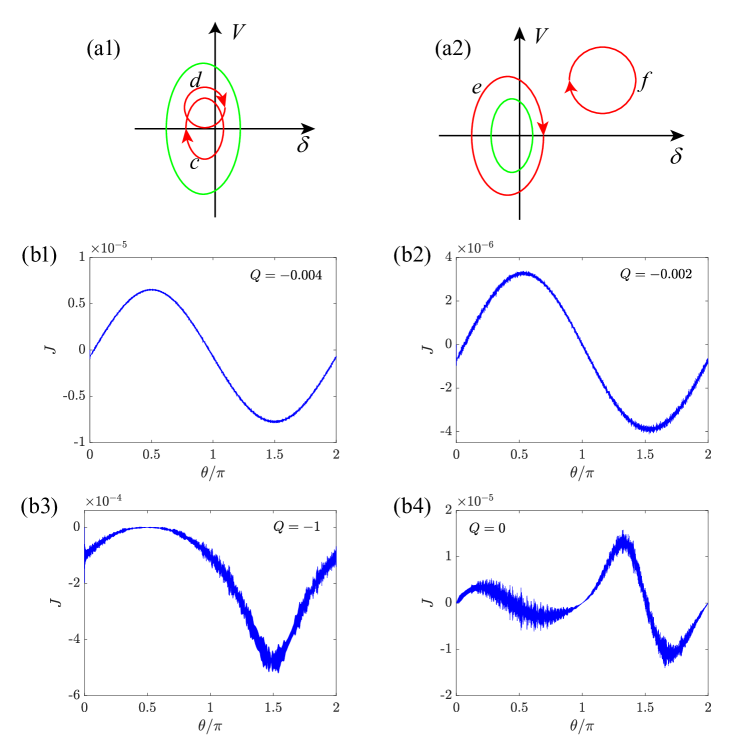
Figure 4: The adiabatic current in Eq. (30) and pumping charge in Eq. (31) of the ground state of the Hamiltonian with nodal lines for different passages. The green loops in (a1) and (a2) are the same nodal line with the parameters $w=0.6,v=-0.3$ and its center is $\left(\delta,V\right)=\left(\delta_{0},0\right)$. $c,d,e$, and $f$ are four different adiabatic loops and the corresponding equations are $c$: $\delta=0.02\sin\left(\omega t\right)+\delta_{0}$, $V=0.04\cos\left(\omega t\right)$; $d$: $\delta=0.02\sin\left(\omega t\right)+\delta_{0}$, $V=0.02\cos\left(\omega t\right)$+0.02; $e$: $\delta=\sin\left(\omega t\right)+\delta_{0}$, $V=2\cos\left(\omega t\right)$ ; $f$: $\delta=0.5\sin\left(\omega t\right)+1$, $V=0.5\cos\left(\omega t\right)+1$ and $\theta=\omega t$. The other parameters are $N=50$, $\omega=0.001$ and the time interval is $t_{l}-t_{l-1}=0.0628$. (b1), (b2), (b3) and (b4) demonstrate the corresponding numerical results for the current and pumping charge. This indicates that if the adiabatic loop encircles the nodal line, the pumping is very close to $-1$, and the pumping charge is very close to $0$ if the nodal line is outside the adiabatic loop.

III Topology of the nodal ellipse

Now, we turn to the question of what happens in the case with nonzero $v+w$, at which the degeneracy points form an ellipse. Here, we would like to emphasize that the nodal line lies in a 2D plane in this work rather than in the 3D space in previous works. For a nodal loop within a 3D space, the pumping charge is studied along a closed passage piercing the nodal loop. Therefore, we will investigate the topology associated with the nodal loop from another aspect. Specifically, how does the pumping charge when an adiabatic loop encloses the ellipse or lies inside the ellipse? In the latter case, the loop does not enclose any degeneracy points, there is no doubt that the pumping charge is zero. However, it is difficult to predict this result for the former case because the total pumping charge depends on the vortex of an individual degenerate point WR1 . In this situation, numerical simulation is an efficient tool providing evidence for theoretical investigation.

A numerical simulation is performed for the time-dependent Hamiltonian with the parameters

$$\delta=R_{1}\cos(\omega t)+\delta_{0},V=R_{2}\sin(\omega t)+V_{0},$$ (27)

which is an ellipse with a center at ($\delta_{0},V_{0}$) in the $\delta-V$ plane. Here, $\omega$ controls the varying speed of the time-dependent Hamiltonian. The computation is performed using a uniform mesh in time discretization. Time $t$ is discretized into $t_{i}$, with $t_{0}=0$ and $t_{M}=T$. For a given initial eigenstate $\left|\phi\left(0\right)\right\rangle$, the time-evolved state is computed using

$$\left|\phi\left(t_{n}\right)\right\rangle=\mathcal{T}\prod\limits_{l=1}^{n}\exp[(-iH\left(t_{l-1}\right)(t_{l}-t_{l-1})]\left|\phi(0)\right\rangle,$$ (28)

where $\mathcal{T}$ is the time-order operator. In the simulation, the value of $M$ is considered sufficiently large to obtain a convergent result. The total pumping charge passing through site $j$ during the time evolution period $T$ can be expressed as

$$Q_{j}\approx\sum_{l=1}^{M}\langle\phi\left(t_{l}\right)|\mathcal{J}_{j}\left(t_{l}\right)\left|\phi\left(t_{l}\right)\right\rangle(t_{l}-t_{l-1}).$$ (29)

and the corresponding average current and average pumping charge are defined as

$$J\left(t_{l}\right)=\frac{1}{N}\sum_{j=1}^{N}\langle\phi\left(t_{l}\right)|\mathcal{J}_{j}\left(t_{l}\right)\left|\phi\left(t_{l}\right)\right\rangle,$$ (30)

$$Q=\frac{1}{N}\sum_{j=1}^{N}Q_{j}.$$ (31)

Due to the translational symmetry of the system, the current and pumping charge across the same type of dimer are identical. However, the average current and pumping charge are favorable for numerical computation.

In principle, the value of $\omega$ should be sufficiently small to fulfill the requirement of quasiadiabatic evolution. In the computation, we select $\omega$ to satisfy the quasiadiabatic condition, under which the obtained pumping charge is not sensitive to a slight change in $\omega$. Fig. 3 and Fig. 4 present the plots of the simulations for two kinds of quasiadiabatic passages with the degeneracy point and nodal line unenclosed and enclosed by a loop, respectively. The instantaneous current and total accumulated charge of the ground state are computed. According to our analysis for the case with $w+v=0$, the final value of the pumping charge $Q$ depends on whether the evolution loop encloses the degeneracy point $(0,0)$ in the $\delta-V$ parameter space. We first demonstrate this point in Fig. 3, which clearly shows that $Q=0$ or $-1$ with high precision for the unenclosed or enclosed circle. We then plot the results for the case with $w+v\neq 0$ in Fig. 4. Notably, we find that the pumping charge $Q=0$ or $-1$ is highly precise for unenclosed or enclosed loops. This strongly implies that the pumping charge can be considered a quasitopological invariant arising from a nodal ellipse. Thus far, this finding has not been verified theoretically.

IV Summary

In summary, we investigated the topology associated with nodal loops in a system without particle number conservation. In addition, the nodal loop lies in a 2D parameter space rather than 3D space. In previous work on a nodal line in 3D space, such as that in Ref. WR1 , the related topology feature was essentially the same as that of an isolated degenerate point. This can be seen from a cross section in 3D space, in which the nodal line reduces to a degenerate point. As an example, we studied the topological pumping charge of a dimerized Kitaev chain with spatially modulated chemical potential. This model has the advantage that it can be mapped into a Rice-Mele model by a partial particle-hole transformation under certain constraints. This motivates us to compute the pumping charge beyond this special case. Numerical simulation of a finite-size chain indicates that the pumping charge is zero for a quasiadiabatic loop within the nodal loop and $\pm 1$ for the passage loop enclosing the nodal loop. This indicates that such a Kitaev model supports topological charge pumping as a demonstration of Chern number. Our findings unveil a hidden topology in a class of Kitaev chains, exploring topological matter from an alternative aspect.

Appendix A Appendix

In this appendix, we derive the spectrum of the Hamiltonian and show that (i) $H$ and $H_{1}$ with $v=-w$ have the same ground state within the region $\left|w\right|<1$ and that (ii) the degenerate lines are a set of conic functions.

(i) In the case of $v+w=0$, we have $\left[H,H_{1}\right]=\left[H_{1},H_{2}\right]=0$. The corresponding core matrices of $H_{1}$ and $H_{2}$ are

$$h_{l}^{k}=\left(\begin{array}[]{cc}A_{l}&-B_{l}\\ B_{l}&-A_{l}\end{array}\right),l=1,2.$$ (32)

Which are defined in the main text. We note that the spectrum $\left\{\varepsilon_{l}^{k},l=1,2\right\}$ of $h_{l}^{k}$ is also symmetric with respect to the zero-energy point; then, one can obtain $\left|\varepsilon_{l}^{k}\right|$ by solving the matrix

$$\left(h_{l}^{k}\right)^{2}=\left(\begin{array}[]{cc}A_{l}^{2}-B_{l}^{2}&B_{l}A_{l}-A_{l}B_{l}\\ B_{l}A_{l}-A_{l}B_{l}&A_{l}^{2}-B_{l}^{2}\end{array}\right).$$ (33)

Taking the unitary transformation

$$u=\frac{1}{\sqrt{2}}\left(\begin{array}[]{cc}1&1\\ 1&-1\end{array}\right),$$ (34)

we have

$$u\left(h_{l}^{k}\right)^{2}u^{{\dagger}}=\left(\begin{array}[]{cc}D_{l}^{+}D_{l}^{-}&0\\ 0&D_{l}^{-}D_{l}^{+}\end{array}\right),$$ (35)

where the diagonal block matrices are

$$D_{l}^{\pm}=A_{l}\pm B_{l}.$$ (36)

Solving the equation

$$\det\left[D_{l}^{+}D_{l}^{-}-\left(\varepsilon_{l}^{k}\right)^{2}I_{2}\right]=0,$$ (37)

we obtain

$$\left(\varepsilon_{1}^{k}\right)^{2} = V^{2}+\left(\varepsilon_{2}^{k}\right)^{2}/w^{2},$$ (38)

$$\left(\varepsilon_{2}^{k}\right)^{2} = w^{2}\left[2\left(\delta^{2}+1\right)\pm f\left(\delta,k\right)\right].$$ (39)

with the function $f\left(\delta,k\right)=\left(\delta^{2}-1\right)\sqrt{2\left(1+\cos k\right)}$. Obviously, we always have $\left|\varepsilon_{1}^{k}\right|>\left|\varepsilon_{2}^{k}\right|$ when $\left|w\right|<1$. As a result, the ground state of $H_{1}$ is also the ground state of $H$.

(ii) For the general case with arbitrary $w$ and $v$, we still have

$$\det\left[D^{+}D^{-}-\left(\varepsilon_{k}\right)^{2}I_{2}\right]=0,$$ (40)

based on a similar analysis. Then, the degeneracy line can be determined by

$$\det\left(D^{+}D^{-}\right)=0.$$ (41)

Here, matrices $D^{\pm}=A\pm B$ can be written in the explicit form

$$D^{\pm}=\left(\begin{array}[]{cccc}V&\Sigma^{\mp}&0&\Delta^{\pm}e^{-ik}\\ \Sigma^{\pm}&-V&\Delta^{\mp}&0\\ 0&\Delta^{\pm}&-V&\Sigma^{\mp}\\ \Delta^{\mp}e^{ik}&0&\Sigma^{\pm}&V\end{array}\right),$$ (42)

where $\Sigma^{\pm}=\left(1-\delta\right)\left(1\pm w\right)$ and $\Delta^{\pm}=\left(1+\delta\right)\left(v\pm 1\right)$. The equation $\det\left(D^{\pm}\right)=0$ requires the vanishing real and imaginary parts of $\det\left(D^{\pm}\right)$, or explicitly

$$\left(V^{2}+\Sigma^{+}\Sigma^{-}-\Delta^{+}\Delta^{-}\right)^{2}+2\Sigma^{+}\Sigma^{-}\Delta^{+}\Delta^{-}$$

$$-\left[\left(\Sigma^{+}\Delta^{+}\right)^{2}+\left(\Sigma^{-}\Delta^{-}\right)^{2}\right]\cos k_{c}=0,$$ (43)

and

$$\left[\left(\Sigma^{+}\Delta^{+}\right)^{2}-\left(\Sigma^{-}\Delta^{-}\right)^{2}\right]\sin k_{c}=0.$$ (44)

Then, the degeneracy lines obey the conditions

$$\left(V^{2}+\Sigma^{+}\Sigma^{-}-\Delta^{+}\Delta^{-}\right)^{2}=\mp\left(\Sigma^{+}\Delta^{+}\pm\Sigma^{-}\Delta^{-}\right)^{2},$$ (45)

for $k_{c}=\pi/2\pm\pi/2$. In the following, we consider only the cases with $\left|w\right|<1$ and $\left|v\right|<1$ for simplicity and without loss of practicality. Within this region, we always have $V^{2}+\Sigma^{+}\Sigma^{-}-\Delta^{+}\Delta^{-}>0$. Then, the conditions for degeneracy lines become

$$\left|V^{2}+\Sigma^{+}\Sigma^{-}-\Delta^{+}\Delta^{-}\right|=\left|\Sigma^{+}\Delta^{+}-\Sigma^{-}\Delta^{-}\right|,$$ (46)

which are simplified to two conic functions

$$\left(\frac{\delta+c_{1}}{a_{1}}\right)^{2}+\left(\frac{V}{b_{1}}\right)^{2}=1,$$ (47)

and

$$\left(\frac{\delta+c_{2}}{a_{2}}\right)^{2}-\left(\frac{V}{b_{2}}\right)^{2}=1,$$ (48)

where the parameters are

$$a_{1} = \frac{2\left(w+v\right)}{4-\left(w-v\right)^{2}},a_{2}=\frac{2}{w+v},$$ (49)

$$b_{1} = \frac{2\left(w+v\right)}{\sqrt{4-\left(w-v\right)^{2}}},b_{2}=2,$$ (50)

$$c_{1} = \frac{w^{2}-v^{2}}{4-\left(w-v\right)^{2}},c_{2}=\frac{v-w}{v+w}.$$ (51)

In conclusion, the nodal lines are conic functions associated with the zero-momentum invariant subspace.

References

- (1) D. J. Thouless, Quantization of particle transport, Phys. Rev. B 27, 6083 (1983).
- (2) Di Xiao, Ming-Che Chang, and Qian Niu, Berry phase effects on electronic properties, Rev. Mod. Phys. 82, 1959 (2010).
- (3) M. Switkes, C. M. Marcus, K. Campman, and A. C. Gossard, An adiabatic quantum electron pump, Science 283, 1905 (1999).
- (4) M. D. Blumenthal, B. Kaestner, L. Li, S. Giblin, T. J. B. M. Janssen, M. Pepper, D. Anderson, G. Jones, and D. A. Ritchie, Gigahertz quantized charge pumping, Nat. Phys. 3, 343 (2007).
- (5) B. Kaestner, V. Kashcheyevs, S. Amakawa, M. D. Blumenthal, L. Li, T. J. B. M. Janssen, G. Hein, K. Pierz, T. Weimann, U. Siegner, and H. W. Schumacher, Single-parameter nonadiabatic quantized charge pumping, Phys. Rev. B 77, 153301 (2008).
- (6) S. Nakajima, T. Tomita, S. Taie, T. Ichinose, H. Ozawa, L. Wang, M. Troyer, and Y. Takahashi, Topological Thouless pumping of ultracold fermions, Nat. Phys. 12, 296 (2016).
- (7) M. Lohse, C. Schweizer, O. Zilberberg, M. Aidelsburger, and I. Bloch, A Thouless quantum pump with ultracold bosonic atoms in an optical superlattice, Nat. Phys. 12, 350 (2016).
- (8) H.-I. Lu, M. Schemmer, L. M. Aycock, D. Genkina, S. Sugawa, and I. B. Spielman, Geometrical pumping with a Bose-Einstein condensate, Phys. Rev. Lett. 116, 200402 (2016).
- (9) J.-T. A. Chiang and Q. Niu, Quantum adiabatic particle transport in optical lattices, Phys. Rev. A 57, R2278(R) (1998).
- (10) Y. Qian, M. Gong, and C. Zhang, Quantum transport of bosonic cold atoms in double-well optical lattices, Phys. Rev. A 84, 013608 (2011).
- (11) L. Wang, M. Troyer, and X. Dai, Topological charge pumping in a one-dimensional optical lattice, Phys. Rev. Lett. 111, 026802 (2013).
- (12) F. Matsuda, M. Tezuka, and N. Kawakami, Topological properties of ultracold bosons in one-dimensional quasiperiodic optical lattice, J. Phys. Soc. Jpn. 83, 083707 (2014).
- (13) F. Mei, J.-B. You, D.-W. Zhang, X. C. Yang, R. Fazio, S.-L. Zhu, and L. C. Kwek, Topological insulator and particle pumping in a one-dimensional shaken optical lattice, Phys. Rev. A 90, 063638 (2014).
- (14) R. Wei and E. J. Mueller, Anomalous charge pumping in a one-dimensional optical superlattice, Phys. Rev. A 92, 013609 (2015).
- (15) Y.-B. Yang, L.-M. Duan, and Y. Xu, Continuously tunable topological pump in high-dimensional cold atomic gases, Phys. Rev. B 98, 165128 (2018).
- (16) F. Matsuda, M. Tezuka, and N. Kawakami, Two-Dimensional Thouless Pumping of Ultracold Fermions in Obliquely Introduced Optical Superlattice, arXiv:1907.10357.
- (17) Y. Zhang, Y. Gao, and D. Xiao, Topological charge pumping in twisted bilayer graphene, Phys. Rev. B 101, 041410(R) (2020).
- (18) R. Wang, C. Li, X. Z. Zhang, and Z. Song, Dynamical bulk-edge correspondence for degeneracy lines in parameter space, Phys. Rev. B 98, 014303 (2018).
- (19) R. Wang, X. Z. Zhang, and Z. Song, Dynamical topological invariant for the non-Hermitian Rice-Mele model, Phys. Rev. A 98, 042120 (2018).
- (20) M. J. Rice and E. J. Mele, Elementary Excitations of a Linearly Conjugated Diatomic Polymer, Phys. Rev. Lett. 49, 1455 (1982).
- (21) A. Y. Kitaev, Unpaired Majorana fermions in quantum wires, Phys. Usp. 44, 131 (2001).
- (22) P. Pfeuty, The one-dimensional Ising model with a transverse field, Ann. Phys. (NY) 57, 79 (1970).
- (23) S. Sachdev, Quantum Phase Transitions (Cambridge University Press, Cambridge, England, 1999).
- (24) T.-P. Choy, J. M. Edge, A. R. Akhmerov, and C. W. J. Beenakker, Majorana fermions emerging from magnetic nanoparticles on a superconductor without spin-orbit coupling, Phys. Rev. B 84, 195442 (2011).
- (25) A. Gorczyca-Goraj, T. Domanski, and M. M. Maska, Topological superconductivity at finite temperatures in proximitized magnetic nanowires, Phys. Rev. B 99, 235430 (2019).
- (26) D. Vodola, L. Lepori, E. Ercolessi, A. V. Gorshkov, and G. Pupillo, Kitaev Chains with Long-Range Pairing, Phys. Rev. Lett. 113, 156402 (2014).
- (27) D. Vodola, L. Lepori, E. Ercolessi, A. V. Gorshkov, and G. Pupillo, Long-range ising and kitaev models: Phases, correlations and edge modes, New. J. Phys. 18, 015001 (2015).
- (28) O. Viyuela, D. Vodola, G. Pupillo, and M. A. Martin-Delgado, Topological massive dirac edge modes and long-range superconducting hamiltonians, Phys. Rev. B 94, 125121 (2016).
- (29) L. Lepori and L. Dell’Anna, Long-range topological insulators and weakened bulk-boundary correspondence, New. J. Phys. 19, 103030 (2017).
- (30) U. Bhattacharya, S.Maity, A. Dutta, and D. Sen, Critical phase boundaries of static and periodically kicked long-range kitaev chain, J. Phys.: Condens. Matter 31, 174003 (2019).
- (31) R. D. King-Smith and D. Vanderbilt, Theory of polarization of crystalline solids, Phys. Rev. B 47, 1651 (1993).
- (32) M. Onoda, S. Murakami, and N. Nagaosa, Hall Effect of Light, Phys. Rev. Lett. 93, 083901 (2004).
- (33) M. Atala, M. Aidelsburger, J. T. Barreiro, D. Abanin, T. Kitagawa, E. Demler, and I. Bloch, Direct measurement of the Zak phase in topological Bloch bands, Nat. Phys. 9, 795 (2013).