Probing the Higgs Portal into Vacuum Stability

Vacuum Stability of the SM and the Higgs Portal

The Higgs Portal into

Vacuum Stability in the Standard Model and Beyond

Abstract

We revisit the stability of the Standard Model vacuum, and investigate its quantum effective potential using the highest available orders in perturbation theory and the most accurate determination of input parameters to date. We observe that the stability of the electroweak vacuum centrally depends on the values of the top mass and the strong coupling constant. We estimate that reducing their uncertainties by a factor of two is sufficient to establish or refute SM vacuum stability at the $5\sigma$ level. We further investigate vacuum stability for a variety of singlet scalar field extensions with and without flavor using the Higgs portal mechanism. We identify the BSM parameter spaces for stability and find sizable room for new physics. We further study the phenomenology of Planck-safe models at colliders, and determine the impact on the Higgs trilinear, the Higgs-to-electroweak-boson, and the Higgs quartic couplings, some of which can be significant. The former two can be probed at the HL-LHC, the latter requires a future collider with sufficient energy and precision such as the FCC-hh.

I Introduction

It is widely appreciated that the Standard Model (SM) of particle physics is incomplete. Yet, clear-cut signatures for new physics at the electroweak scale are missing, despite of extensive experimental searches and a variety of anomalies in the data. Also, theory guidance for top-down model building from first principles beyond the paradigm of effective theories is scarce. Therefore, it has been proposed to revisit the metastability of the SM vacuum Degrassi:2012ry and to turn it into a bottom-up model building task Hiller:2022rla ; Hiller:2023bdb . While the onset of metastability in the SM around $10^{10}\,\text{GeV}$ is a high energy effect – though still far below the quantum gravity scale – its remedy may arise from new physics at any scale below, possibly as low as a TeV. At the same time, new physics modifications of the Higgs potential may also affect interaction vertices of the Higgs particle, thus offering additional opportunities for indirect tests of stability at present and future colliders such as the (high-luminosity) Large Hadron Collider LHC (HL-LHC) ATLAS:2019mfr , the Future Circular Collider (FCC) FCC:2018byv , the Chinese Electron Positron Collider (CEPC) CEPCStudyGroup:2018ghi , the International Linear Collider Project (ILC) ILC:2019gyn or a muon collider Casarsa:2023vqx . In this light, the aim of this paper is threefold:

Firstly, we revisit the stability of the SM vacuum, and investigate its quantum effective potential using the highest available orders in perturbation theory and the most accurate determination of input parameters to date. We find that the stability centrally depends on the values of the top mass and the strong coupling constant, their uncertainties Workman:2022ynf , and correlation CMS:2019esx . We estimate that reducing their uncertainties by a factor of two is sufficient to establish or refute stability at the $5\sigma$ level.

Secondly, we systematically investigate the stability of scalar field extensions with and without flavor, using the Higgs portal mechanism. This includes the addition of real, complex, $O(N)$, or $SU(N)\times SU(N)$ symmetric singlet scalar fields $S$, their self-interactions, and their renormalizable portal couplings $\sim(H^{\dagger}H)(S^{\dagger}S)$ with the Higgs $H$. For either of these, we identify the BSM parameter spaces of masses and couplings for SM extensions to be “Planck-safe” – meaning stable up to or at the Planck scale, and free of subplanckian Landau poles – and uncover sizable room for new physics. Results are achieved by extensive studies of the two-loop RG running of couplings between the scale of new physics and the Planck scale using the precision tool ARGES Litim:2020jvl . Our methodology has been developed in a series of earlier works Hiller:2019mou ; Hiller:2020fbu ; Bissmann:2020lge ; Bause:2021prv ; Hiller:2022rla ; PlanckSafeQuark , inspired by models of particle physics with controlled interacting UV fixed points Litim:2014uca ; Litim:2015iea ; Bond:2016dvk ; Buyukbese:2017ehm ; Bond:2017lnq ; Bond:2017suy ; Bond:2017tbw ; Bond:2017wut ; Kowalska:2017fzw ; Bond:2018oco ; Bond:2019npq ; Fabbrichesi:2020svm ; Bond:2021tgu . Previous studies of the Higgs portal include BSM models with a real Falkowski:2015iwa ; Khan:2014kba ; Han:2015hda ; Garg:2017iva , complex Gabrielli:2013hma ; Elias-Miro:2012eoi ; Gonderinger:2012rd ; Costa:2014qga ; Khoze:2014xha ; Anchordoqui:2012fq , or charged scalar(s) Bandyopadhyay:2016oif ; Bandyopadhyay:2021kue ; Chakrabarty:2020jro ; Hamada:2015bra , models with additional BSM Yukawa couplings  Latosinski:2015pba ; Hiller:2019mou ; Hiller:2020fbu ; Bause:2021prv ; Xiao:2014kba ; Dhuria:2015ufo ; Salvio:2015jgu ; Son:2015vfl ; DuttaBanik:2018emv ; Borah:2020nsz and two-Higgs-doublet models Chowdhury:2015yja ; Khan:2015ipa ; Ferreira:2015rha ; Ferreira:2015pfi ; Bhattacharya:2019fgs ; Swiezewska:2015paa ; Chakrabarty:2016smc ; Schuh:2018hig ; Bagnaschi:2015pwa (for an overview see Hiller:2022rla and references therein).

Thirdly, we investigate the modifications of the Higgs potential dictated by Planck-safe SM extensions and their phenomenology at colliders. In particular, we determine the impact of new physics on the Higgs trilinear, the Higgs-to-electroweak-boson, and the Higgs quartic couplings, which can be sizable. We show that the former two can already be probed at the HL-LHC ATLAS:2019mfr , whereas the latter will require a future collider with sufficient energy and precision such as the FCC-hh FCC:2018byv .

The paper is organized as follows. We begin with an update of the SM quantum effective potential and its stability in terms of the most critical input parameters (Sec. II). This is followed by a study of the Higgs portal for a variety of singlet scalar field extensions with and without flavor, and their BSM parameter spaces for safe and stable extensions up to the Planck scale (Sec. III). We further work out the phenomenology of stable SM extensions, in particular their impact on the Higgs trilinear, quartic, and couplings to the $Z$ boson, and their signatures at present and future colliders (Sec. IV). We close with a brief discussion of results and some conclusions (Sec. V). Four appendices contain further details of the SM stability analysis (App. A), conventions and terminology (App. B), scalar mixing (App. C), and constraints from unitarity (App. D).

II Revisiting SM Vacuum Stability

Since the discovery of the Higgs boson ATLAS:2012yve ; CMS:2012qbp the meta-stability of its potential has been evidenced Degrassi:2012ry ; Buttazzo:2013uya . The metastability appears to be non-pathological in that the tunnel rate is comparable with the age of the universe Buttazzo:2013uya . Also, absolute stability has neither been excluded conclusively due to underlying uncertainties of SM observables. Ever since these early works, important strides have been made in both theory and experiment improving this prediction. Thus, a high-precision determination of the region of vacuum stability in the SM is warranted and will be conducted here, enhancing previous studies, e.g. Degrassi:2012ry ; Alekhin:2012py ; Buttazzo:2013uya ; Andreassen:2014gha ; Bednyakov:2015sca ; Chigusa:2018uuj .

II.1 Input

Progress on the experimental side consists of improved precision for all input observables that determine vacuum stability in the SM. These include the Higgs, top and $Z$ pole masses $M_{h,t,Z}$, the 5-flavor strong coupling $\alpha_{s}^{(5)}(\mu=M_{Z})$, the fine-structure constant $\alpha_{e}$ and the hadronic contribution to its running $\Delta\alpha_{e}^{(5)}(\mu=M_{Z})$, Fermi’s constant $G_{F}$, $\overline{\text{MS}}$ quark masses $m_{b}(\mu=m_{b})$, $m_{c}(\mu=m_{c})$, $m_{u,d,s}(\mu=2\,\text{GeV})$ and lepton pole masses $M_{e,\mu,\tau}$. Their central values and uncertainties are taken from the 2023 update of the PDG Workman:2022ynf .

Progress on the theory side consists of several streams. Specifically, using Alam:2022cdv , all running SM parameters and their uncertainties are determined from the input observables at a reference scale

$$\mu_{\text{ref}}=200~{}\text{GeV}\,.$$ (1)

The precision of this procedure is an improvement upon Buttazzo:2013uya , an overview of all loop contributions is found in Martin:2019lqd . In particular, five loop logarithmic resummations are conducted Baikov:2012zm ; Baikov:2016tgj ; Herzog:2017ohr ; Luthe:2017ttg ; Chetyrkin:2017bjc while threshold and matching corrections to the light quark masses and gauge couplings are considered up to four loops in QCD Melnikov:2000qh ; Martin:2018yow . The pole masses of the top quark, $Z$ and Higgs boson are matched at full two loop precision with leading three-loop corrections Martin:2014cxa ; Martin:2015rea ; Martin:2016xsp ; Martin:2022qiv .

SM vacuum stability is established if the quantum effective potential is bounded from below. We employ an RG-improved ansatz

$$\frac{1}{(4\pi)^{2}}V_{\text{eff}}=\frac{1}{4}\alpha_{\lambda,\text{eff}}(\alpha_{i})\ h^{4}\left(\frac{1}{8\pi^{2}\alpha_{t}}\frac{h}{\mu}\right)^{4\gamma/(1-\gamma)}\,,$$ (2)

where $h$ is the Higgs field and $\gamma$ its anomalous dimension. We denote all running couplings by

$$\alpha_{i}=\frac{z_{i}^{2}}{(4\pi)^{2}}\text{ with }z_{i}=g_{1,2,3},\text{ or }y_{t,b,c,s,u,d,\tau,\mu,e}\,$$ (3)

as well as $\alpha_{\lambda}=\lambda/(4\pi)^{2}$ for the Higgs self-interaction in the tree-level potential. Vacuum stability is independent of the field values $h$ and requires

$$\alpha_{\lambda,\text{eff}}>0\,,$$ (4)

as all other factors in (2) are manifestly positive. The effective coupling $\alpha_{\lambda,\text{eff}}$ is obtained by matching (2) to fixed-order calculations of the effective potential Ford:1992pn ; Martin:2013gka ; Martin:2014bca ; Martin:2015eia ; Martin:2017lqn ; Martin:2018emo which are evaluated at constant field value $h=8\pi^{2}\alpha_{t}\,\mu$. The first loop order reads

$$\alpha_{\lambda,\text{eff}}= {}\ \alpha_{\lambda}+\frac{3}{16}(\alpha_{1}+\alpha_{2})^{2}\left(\ln\frac{\alpha_{1}+\alpha_{2}}{2\alpha_{t}}-\frac{5}{6}\right)$$ (5)

$${}+4\,\alpha_{\lambda}^{2}\left(\ln\frac{4\alpha_{\lambda}}{\alpha_{t}}-\frac{3}{2}\right)+\frac{3}{8}\alpha_{2}^{2}\left(\ln\frac{\alpha_{2}}{2\alpha_{t}}-\frac{5}{6}\right)$$

$$-\sum_{f}N_{f}\alpha_{f}^{2}\left(\ln\frac{\alpha_{f}}{\alpha_{t}}-\frac{3}{2}\right)+\mathcal{O}(\text{2 loop}),$$

where the sum in the last line runs over all fermions flavors $f=t,b,c,s,u,d,\tau,\mu,e$ and $N_{f}$ are the respective color multiplicities. Apart from the well-known results (5), we include electroweak, strong, top and scalar contributions at two loops Ford:1992pn ; Martin:2018emo , strong and top contributions at three loops Martin:2013gka ; Martin:2017lqn and QCD contributions at four loops Martin:2015eia , all in Landau gauge and with Goldstone resummation Martin:2014bca ; Martin:2017lqn . The effective potential is stable if the coupling $\alpha_{\lambda,\text{eff}}$ does not turn negative under RG evolution. We study the evolution explicitly between $\mu_{\text{ref}}\leq\mu\leq M_{\text{Pl}}{}$, where we employ four loop running for gauge couplings Davies:2019onf ; Davies:2021mnc ; Bednyakov:2021qxa , three-loop for Yukawa Bednyakov:2012en ; Davies:2021mnc ; Bednyakov:2021qxa as well as quartic Chetyrkin:2013wya ; Bednyakov:2014pia interactions. On top of that, 5-loop QCD corrections for the strong coupling beta function Baikov:2016tgj ; Herzog:2017ohr ; Luthe:2017ttg ; Chetyrkin:2017bjc as well and four loops for Yukawas and quartic Chetyrkin:2016ruf are utilized.

II.2 Results

We find that at the reference scale $\mu_{\text{ref}}$ the effective quartic $\alpha_{\lambda,\text{eff}}(\mu_{\text{ref}})$ is enhanced by $17\%$ over its tree level value $\alpha_{\lambda}(\mu_{\text{ref}})$. Studying the RG evolution between $\mu_{\text{ref}}\leq\mu\leq M_{\text{Pl}}{}$, instability is already manifest in the tree-level potential, as $\alpha_{\lambda}$ turns negative at $\Lambda_{0}\approx 9\cdot 10^{10}$ using PDG central values. Taking into account quantum corrections to the potential, $\alpha_{\lambda,\text{eff}}$ still turns negative before the Planck scale around $\Lambda_{0,\text{eff}}\approx 2\cdot 10^{11}$ GeV. However, the coupling remains only slightly negative $\alpha_{\lambda,\text{eff}}\gtrsim-10^{-4}$, hinting at metastability of the potential. If quantum gravity effects are neglected, $\alpha_{\lambda,\text{eff}}$ turns positive again after the Planck scale. The RG evolution of $\alpha_{\lambda,\text{eff}}$ (solid, including $5\sigma$ uncertainty bands form $M_{t}$) and $\alpha_{\lambda}$ (dashed, using central values) are displayed in Fig. 1.

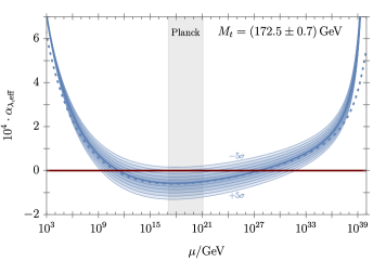
Figure 1: Shown is the running quartic coupling $\alpha_{\lambda,\text{eff}}$ characterizing the quantum effective potential at the RG scale $\mu$, using the PDG central value of the top mass (thick line) and five standard deviations in either direction (thin lines), while the gray band indicates the Planck scale. For comparison, we also show the running of the quartic coupling $\alpha_{\lambda}$ of the tree-level potential (thick dashed line). Effective potentials for which $\alpha_{\lambda,\text{eff}}$ stays positive are stable.

Obs.	Value	$\alpha_{\lambda}>0$		$\alpha_{\lambda,\text{eff}}>0$
$M_{h}/\text{GeV}$	$125.25(17)$	$128.22$	$+17.5\sigma$	$128.10$	$+16.7\sigma$
$M_{t}/\text{GeV}$	$172.5(7)^{\ddagger}$	$169.62$	$-\phantom{0}4.1\sigma$	$169.74$	$-\phantom{0}3.9\sigma$
	$172.69(30)^{\dagger}$		$-10.3\sigma$		$-\phantom{0}9.8\sigma$
	$170.5(8)$	$167.85$	$-\phantom{0}3.3\sigma$	$167.97$	$-\phantom{0}3.2\sigma$
$m_{t}/\text{GeV}$	$162.5(^{+2.1}_{-1.5})$	$160.0\phantom{0}$	$-\phantom{0}1.7\sigma$	$160.1\phantom{0}$	$-\phantom{0}1.6\sigma$
$\alpha_{s}^{(5)}(M_{Z})$	$0.1180(9)$	$0.1255$	$+\phantom{0}8.3\sigma$	$0.1252$	$+\phantom{0}8.0\sigma$
	$0.1135(^{+21}_{-17})$	$0.1203$	$+\phantom{0}3.2\sigma$	$0.1200$	$+\phantom{0}3.1\sigma$

Table 1: Strong coupling, Higgs or top mass and their uncertainty from PDG Workman:2022ynf (white fields) as well as CMS analysis CMS:2019esx (gray fields). For each observable, the shift around the central values from Workman:2022ynf or CMS:2019esx required to stabilize the tree level $(\alpha_{\lambda}>0)$ or quantum effective potential $(\alpha_{\lambda,\text{eff}}>0)$ in the SM before the Planck scale is given. The value $m_{t}$ is the $\overline{\text{MS}}$ mass of the top at the scale $m_{t}$. The PDG top pole masses $M_{t}$ extracted from cross section measurements^‡ and Monte-Carlo fits^† are both listed.

An overview of the most sensitive observables to determine the stability of the SM potential is collected in Tab. 1. The Higgs pole mass is essential to extract $\alpha_{\lambda}(\mu_{\text{ref}})$ and thus its uncertainty has the highest impact at tree-level for $\alpha_{\lambda,\text{eff}}(\mu_{\text{ref}})$. However, the uncertainty of $M_{h}$ is modest and instability arises as a result of RG running above $\mu_{\text{ref}}$ : due to the technical non-naturalness of $\alpha_{\lambda}$, the coupling is subdominant in its own RG evolution, and the influence on stability is weak. On the other hand, $\alpha_{t}$ and $\alpha_{3}$, corresponding to the top mass and $\alpha_{s}^{(5)}(M_{Z})$, are the largest couplings at $\mu_{\text{ref}}$ and dominate the running. To stabilize the Higgs, $\alpha_{s}^{(5)}(M_{Z})$ requires an $8\sigma$ upward shift from the 2023 PDG world average. Note however that many individual studies summarized in Workman:2022ynf quote much larger uncertainties, often resulting in a less than $5\sigma$ shift. The critical role of the strong coupling may appear surprising given that its influence on the effective potential as well as the running is loop-suppressed. This suppression, however, is effectively compensated by $\alpha_{3}$ (and $\alpha_{t}$) being numerically large compared to the other SM gauge and Yukawa couplings.

Alternatively, a smaller value of the top mass may also entail vacuum stability in the SM. The PDG provides three world averages for the top mass. The pole mass extracted from cross section measurements, $M_{t}=(172.5\pm 0.7)~{}\text{GeV}$, implies that a $3.9\sigma$ downwards shift from its central value stabilizes the Higgs potential. A secondary top mass estimate $M_{t}=(172.69\pm 0.30)$ GeV stems from template fits of kinematic distributions sensitive to the top-quark pole mass Hoang:2020iah . These template fits are based on a modeling of top-quark production and decay dynamics in Monte Carlo event generators. The small uncertainty requires a $10\sigma$ shift to achieve stability. The recent update Dehnadi:2023msm suggests that the difference in uncertainties of both pole mass predictions is similar to the uncertainty differences among the various Monte-Carlo generators. Finally, the PDG also quotes an $\overline{\text{MS}}$ top mass value $m_{t}(\mu=m_{t})$, which has a large uncertainty of about $1\%$ that would allow stabilization of the Higgs potential with a $1.6\sigma$ shift.

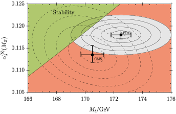
Figure 2: Regions of stability for the SM Higgs potential as a function of the top mass $M_{t}$ and the strong coupling constant $\alpha_{s}^{(5)}(M_{Z})$. Upper panel: 2023 PDG central values and uncertainties Workman:2022ynf , including the first five $1\sigma$ uncertainty rings (thin lines). The top mass from cross-section measurements is utilized. Lower panel: CMS central values with correlated uncertainties CMS:2019esx and $1\sigma$ rings (dashed lines), in comparison with the PDG. Color-coding indicates stability ($\alpha_{\lambda,\text{eff}}(\mu)\geq 0$, green) or otherwise (red/gray).

If PDG uncertainties in both top mass and strong coupling are combined in quadrature less then a $4\sigma$ deviation from the central values are required to achieve stability, see Fig. 2. However, this neglects correlations between the observables, which may play a critical role in determining the stability of the SM Higgs vacuum.

The correlation was taken into account by the CMS analysis CMS:2019esx . Here the central value of $\alpha_{s}^{(5)}(M_{Z})$ and $M_{t}$ are smaller than the PDG world averages, and the uncertainty for $\alpha_{s}^{(5)}(M_{Z})$ is significantly larger. Moreover, $\alpha_{s}^{(5)}(M_{Z})$ and $M_{t}$ in CMS:2019esx are individually $3\sigma$ and in combination $2\sigma$ away from the region of absolute stability. The PDG (upper plot) and CMS (lower plot) determinations of $\alpha_{s}$ versus $M_{t}$ are depicted in Fig. 2.

Given the present state of affairs, one may also turn the question around and ask how much accuracy is required individually in the determination of the top mass and the strong coupling constant to establish the absence of SM Higgs stability at the $5\sigma$ level or above. Assuming that central values do not change, we find that a $5\sigma$ signature necessitates the uncertainty in the top mass $M_{t}$ to come down to the $500-600$ MeV range. Similarly, the uncertainty in $\alpha_{s}^{(5)}$ would have to come down to the $(14-15)\cdot 10^{-4}$ range. Based on the presently reported errors (see Tab. 1), it is conceivable that these targets are in reach in the near future.

We briefly comment on the influence of other SM input. The electroweak gauge couplings $\alpha_{1,2}(\mu_{\text{ref}})$ are larger than $\alpha_{\lambda}(\mu_{\text{ref}})$, and therefore have sizable impact on its RG evolution. However, the values of $\alpha_{1,2}$ are extracted from electroweak precision observables, $\alpha_{e}$, $G_{F}$, $M_{Z}$ and $\Delta\alpha_{\text{had}}^{(5)}(M_{Z})$ to the running fine structure constant, which have too small of an uncertainty to matter at the level of $M_{t,h}$ and $\alpha_{s}^{(5)}(M_{Z})$ for the evolution of $\alpha_{\lambda}$ and its sign. In particular, the current tension Parker:2018vye ; Morel:2020dww in the determination of the fine structure constant is insignificant in the context of vacuum stability. The $W$ pole mass has a higher uncertainty than the one of the $Z$, and is therefore not included in the analysis. The remaining input parameters, such as quark and lepton masses, are too small to play a role for the effective potential and stability analysis.

In summary, we have sharpened the evidence for the metastability of the SM vacuum. At this point, however, a completely stable SM cannot be excluded at a $5\sigma$ confidence level, as this would require higher precision in the determinations of the top mass, the strong coupling, and their uncertainties and correlation. We also emphasize that stability is largely dominated by RG effects, and that the role of finite-order corrections to the effective potential is minor. This supports the view that the stability of SM extensions may very well be extracted from RG studies of the tree-level potential. This will be our main search strategy from here on.

III Stability via Higgs Portals

In this section, we change gear and take the metastability of the SM as a model building task to find stable vacua all the way up to the Planck scale. Our focus is on a variety of singlet scalar field extensions with and without flavor, and the prospects for stability through the Higgs portal mechanism.

III.1 Higgs Portal Mechanism

We consider models in which the SM is extended by a scalar singlet sector under the SM $SU(3)_{C}\times SU(2)_{L}\times U(1)_{Y}$ gauge group. Such scalars, generically denoted by real components $S_{i}$, allow for a well-known renormalizable portal interaction

$${\cal L}\supset\sum_{i}\delta_{i}\,(H^{\dagger}H)(S_{i}\!{}^{\intercal}\!S_{i})$$ (6)

with the SM Higgs doublet $H$ via canonically marginal portal couplings $\delta_{i}$. This Higgs portal most directly affects the Higgs sector and can cure metastability Machacek:1984zw . Previous works considering such models include e.g. Falkowski:2015iwa ; Khan:2014kba ; Han:2015hda ; Garg:2017iva ; Gabrielli:2013hma ; Elias-Miro:2012eoi ; Gonderinger:2012rd ; Costa:2014qga ; Khoze:2014xha .

In particular, the Higgs portal affects the RG evolution of Higgs quartic $\lambda$, which enters in the scalar potential term as $\lambda(H^{\dagger}H)^{2}$, at 1-loop order

$$\beta_{\lambda}=\beta^{\text{SM}}_{\lambda}+\sum_{i}2\,N_{i}\,\alpha_{\delta_{i}}^{2}\,,$$ (7)

where $\beta_{\lambda}\equiv\frac{\text{d}\alpha_{\lambda}}{\text{d}\ln\mu}$ denotes the beta-function of $\alpha_{\lambda}$, and $N_{i}$ denotes the number of real scalar components in each $S_{i}$, such that (6) is compatible with a $O(N_{i})$ symmetry for each $S_{i}$. Here and in the following we denote for any quartic coupling

$$\alpha_{q}=\frac{q}{(4\pi)^{2}},\quad\text{ with }q=\lambda,\delta,...$$ (8)

and (3) for the gauge and Yukawa couplings. Therefore, at a scale $\Lambda$ at or above the electroweak one,

$$\alpha_{\lambda}(\Lambda)-\alpha_{\lambda}^{\text{SM}}(\Lambda)\propto\sum_{i}2\,N_{i}\,\alpha_{\delta_{i}}^{2}>0\,,$$ (9)

that is, the portal contribution increases the Higgs quartic relative to its SM value.

The $\beta$-function of the Higgs portal coupling is technically natural, i.e. $\beta_{\delta}\propto\alpha_{\delta}$. Thus, if vanishing, $\alpha_{\delta}$ cannot be switched on by quantum fluctuations. As a consequence there cannot be any RG induced sign changes of $\alpha_{\delta}$ in the running either. As further discussed in concrete models in the following, the RG evolution of $\alpha_{\delta}$ is governed by both the SM as well as the BSM sector. The details of the latter depends on symmetries; in general there exist several quartic interactions among the BSM scalars. However, the pure BSM quartics enter $\beta_{\lambda}$ directly only starting from three loops, and are always mediated by the portal coupling $\alpha_{\delta}$ Machacek:1984zw . Therefore, the pure BSM scalar potential decouples from the Higgs portal mechanics for sufficiently small couplings. On the other hand, we find that, due to the interplay of BSM quartics with the portal, even small values of $\delta$ induce stability once the pure BSM quartics are sufficiently large.

For the RG-analysis and numerics to identify stability regions we follow closely Hiller:2022rla to which we refer for further details. In particular, we make use of the SM couplings from Alam:2022cdv and apply full 2-loop running of all couplings in our BSM models. The central goal of this work is to identify parameter configurations in scalar SM extensions that allow for Planck safety, that is a RG flow from the new physics scale $\mu_{0}=M_{s}\gtrsim 1\,\text{TeV}$ - where $M_{s}$ denotes the physical mass of the BSM scalar(s) - up to the Planck scale $M_{\text{Pl}}\simeq 10^{19}\,\text{GeV}$ without poles and vacuum instabilities. These Planck-safe parameter configurations span the BSM ciritical surface at the matching scale. If in the RG evolution all (tree-level) vacuum stability conditions are fulfilled all the way to the Planck scale we speak of strict Planck safety. On the other hand, if a RG flow features intermediate metastabilities in the Higgs potential but a stable potential at the Planck scale we speak of soft Planck safety, see App. B for details.

The remainder of this section deals with vacuum stability in BSM extensions with $O(N)$ global symmetry (Sec. III.2), models with a single scalar singlet field (Sec. III.3), the incompatibility of a negative portal with Planck-safety (Sec. III.4), flavorful BSM extensions with more delicate symmetries (Sec. III.5) and the availability of negative BSM quartics for these (Sec. III.6).

III.2 ${O(N_{S})}$ Symmetric Scalars

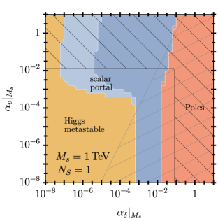
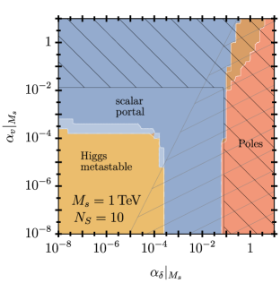
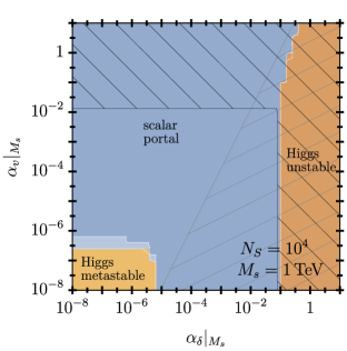
Figure 3: BSM critical surface for the $O(N_{S})$ model with $N_{S}=1,10,100$ and $10^{4}$ generations of real scalar singlets spanned by the pure BSM quartic $\alpha_{v}(M_{s})$ and the Higgs portal $\alpha_{\delta}(M_{s})$. Red areas correspond to a RG evolution featuring Landau poles below the Planck scale. Brown indicates instabilities in the Higgs potential ($\min\alpha_{\lambda}(\mu)\leq-10^{-4}$). Gray regions feature an unstable BSM scalar potential i.e. violation of (11) at some scale $\mu$ before $M_{\text{Pl}}$. Yellow regions correspond to a SM-like RG evolution with $-10^{-4}\leq\min\alpha_{\lambda}(\mu),\,\alpha_{\lambda}(M_{\text{Pl}})\leq 0$ hinting a metastable Higgs. Dark (light) blue areas correspond to a strictly (softly) Planck-safe RG evolution with a stable potential all the way up to (at) $M_{\text{Pl}}$, see App. B. Hatched black areas violate tree-level perturbative unitarity (15), while gray, lightely hatched ones are experimentally excluded by (31) on the scalar mixing angle, see Sec. IV for details.

The simplest global symmetry group a SM extension with $N_{S}$ real BSM scalars can exhibit is $O(N_{S})$, which implies a mass parameter $\mu_{S}$, a portal coupling $\delta$ as well as BSM quartic $v$. The scalar potential

$$V_{O(N_{S})}= -\frac{1}{2}\mu_{H}^{2}H^{\dagger}H-\frac{1}{2}\mu_{S}^{2}S^{T}S+\lambda(H^{\dagger}H)^{2}$$ (10)

$$+v(S^{T}S)^{2}+\delta\,(H^{\dagger}H)(S^{T}S),$$

is stable if

$$\qquad\lambda>0,\qquad v>0,\qquad\delta>-2\sqrt{\lambda v}.$$ (11)

For $N_{S}=1$ the global symmetry becomes a $\mathbb{Z}_{2}$. The setup (10) describes also $\tfrac{1}{2}N_{S}$ complex scalars with a $U(N_{S}/2)$ global symmetry. For more delicate global symmetries, there might be additional quartic interactions beyond the BSM scalar portal $\delta$ and self-coupling $v$. However, the potential (10) can be recovered by switching off all couplings that violate the $O(N_{S})$ symmetry.

The RG-analysis and numerics how to identify stability regions is described in App. B and Hiller:2022rla , to which we refer for further details. The Higgs portal mechanics arises already at 1-loop via (7), with $i=1$ and $N_{1}=N_{S}$. Including also the two-loop contribution $\beta_{\lambda}$ reads

$$\beta_{\lambda}= \beta^{\text{SM}}_{\lambda}+\beta^{\text{BSM},(1)}_{\lambda}+\beta^{\text{BSM},(2)}_{\lambda},$$ (12)

$$\beta^{\text{BSM},(1)}_{\lambda}= +2N_{S}\,\alpha_{\delta}^{2},$$

$$\beta^{\text{BSM},(2)}_{\lambda}= -4\,N_{S}(4\,\alpha_{\delta}+5\alpha_{\lambda})\alpha_{\delta}^{2}.$$

The pure BSM quartic $\alpha_{v}$ does not contribute to $\beta_{\lambda}$ at 1- and 2-loop Machacek:1984zw . However it contributes positively at 1-loop to $\beta_{\delta}$ via

$$\beta_{\delta}= \beta^{(1)}_{\delta}+\beta^{(2)}_{\delta},$$ (13)

$$\beta^{(1)}_{\delta}\subset [+8(2+N_{S})\alpha_{v}]\alpha_{\delta},$$

$$\beta^{(2)}_{\delta}\subset [-160(2+N_{S})\alpha_{v}^{2}-96N_{S}\,\alpha_{v}\alpha_{\delta}]\alpha_{\delta}.$$

Thus, a sizable $\alpha_{v}$ can indirectly also cause an uplift of $\alpha_{\lambda}$ by inducing an uplift in $\alpha_{\delta}$. Recall that the full $\beta_{\delta}\propto\alpha_{\delta}$ is technically natural, we just omitted the terms involving SM couplings as they are not relevant for demonstrating the discussed stabilization mechanisms. For completeness we also give the beta function at one and two loop for the pure BSM quartic

$$\beta_{v} =\beta^{(1)}_{v}+\beta^{(2)}_{v}\,,$$ (14)

$$\beta^{(1)}_{v} =(8N_{S}+64)\alpha_{v}^{2}+2\alpha_{\delta}^{2}\,,$$

$$\beta^{(2)}_{v} =-(2688+576N_{S})\alpha_{v}^{3}-16\alpha_{\delta}^{3}-80\alpha_{v}\alpha_{\delta}^{2}$$

$$\phantom{=\ }+4(\alpha_{1}+3\alpha_{2}-3\alpha_{b}-3\alpha_{t})\alpha_{\delta}^{2}\,.$$

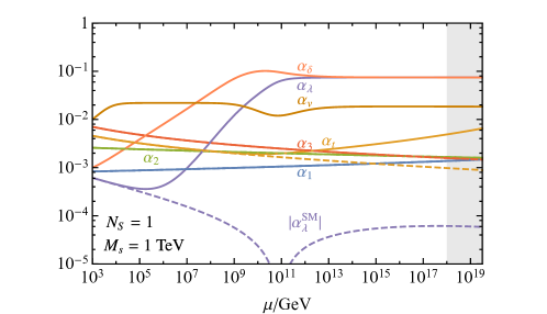
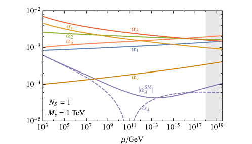
Figure 4: Two-loop renormalization group flow in the SM (dashed lines) and the scalar $O(N_{S})$ model (solid lines) for $N_{S}=1$, $M_{s}=1\text{ TeV}$, $(\alpha_{\delta},\,\alpha_{v})|_{M_{s}}=(10^{-3},\,10^{-2})$ (top) and $(\alpha_{\delta},\,\alpha_{v})|_{M_{s}}=(10^{-3},\,10^{-4})$ (bottom). In the upper plot quartic couplings are trapped in a walking regime before the Planck scale, whereas in the lower plot the running to $M_{\text{Pl}}$ occurs within a weakly coupled regime without walking.

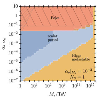
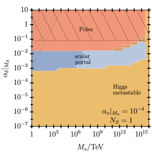
Figure 5: BSM critical surface in the $M_{s}-\alpha_{\delta}(M_{s})$-plane in a minimal BSM model featuring $N_{S}=1$ real BSM scalars and $O(N_{S})$ symmetry for fixed $\alpha_{v}(M_{s})=10^{-2}$ (top) and $\alpha_{v}(M_{s})=10^{-4}$ (bottom). Same color coding as Fig. 3.

In Fig. 3, the BSM critical surface in $\alpha_{\delta}-\alpha_{v}$ space is displayed for different field multiplicities $N_{S}$ and mass $M_{s}=1\,\text{TeV}$. Generically, the metastability of the Higgs potential is cured if $\alpha_{v}$ or $\alpha_{\delta}$ are sufficiently large. However, too large values of $\alpha_{\delta}$ lead to the loss of Higgs stability and to subplanckian Landau poles. Due to the term $N_{S}\,\alpha_{\delta}^{2}$ in (12) an increase of $N_{S}$ generically lowers the minimal values of $\alpha_{\delta}$ and $\alpha_{v}$ required to stabilize the Higgs. We emphasize that even a feeble portal coupling suffices to achieve stability due to the indirect stabilization from a large $\alpha_{v}(M_{s})$.

Also shown (dark hatched) in Fig. 3 and subsequent figures are constraints from tree-level perturbative unitarity Dawson:2021jcl

$$\alpha_{\lambda}\lesssim\frac{1}{6\pi},\quad\alpha_{v}\lesssim\frac{1}{24\pi},\quad\alpha_{\delta}\lesssim\frac{1}{4\pi},\quad$$ (15)

as well as constraints from mixing between the Higgs and the BSM scalar (lighter, gray hatched). The latter requires the BSM scalar to acquire a VEV, see App. C and App. D for details. While the unitarity bounds limit couplings to be rather perturbative, outside of which theoretical control ceases anyway, the implications of the Higgs being an admixture can lead to additional constraints.

Depending on the the parameters $\alpha_{\delta},\,\alpha_{v}$ and $N_{S}$ the stabilization of the Higgs potential may occur either within a weakly coupled or a walking regime. The latter refers to an RG flow where a subset of couplings is interlocked at sizable, fixed values for several orders of magnitude, see Fig. 4 (top figure). Walking regimes are a well known phenomenon that has already been observed in earlier works Hiller:2020fbu ; Hiller:2022rla . They occur due to the presence of a pseudo fixed point, i.e. a nearby fixed point of the RG flow in the complex plane of couplings. The walking greatly enhances the parameter space that exhibits Planck safety, and its occurrence with respect to non-walking is more pronounced at larger $\alpha_{\delta},\,\alpha_{v}$ and $N_{S}$. Moreover, larger coupling values work without encountering subplanckian Landau poles.

We find that for TeV-ish BSM scalars a stable potential (17) at large $N_{S}$ is roughly obtained for

$$10^{-3}/\sqrt{N_{S}}\lesssim\alpha_{\delta}\lesssim 10^{-1}$$ (16)

or $$N_{S}\,\alpha_{v}\gtrsim 10^{-2}~{}\text{and}~{}\log\alpha_{\delta}\gtrsim-0.16\,N_{S}-6.6$$

$$\qquad\qquad\qquad\qquad\;\,(\log\alpha_{\delta}\gtrsim-0.93\,N_{S}-6.1)$$

for strict (soft) Planck safety, see also Fig. 3. The second condition in (LABEL:eq:ON-cond) corresponds to an indirect stabilization of the Higgs potential. The relatively large value of $\alpha_{v}(M_{s})$ induces a significant RG growth in $\alpha_{\delta}$ which is then sufficient to render $\alpha_{\lambda}$ positive up to $M_{Pl}$ even for tiny $\alpha_{\delta}(M_{s})$. Note that the allowed ranges for $\alpha_{v}(M_{s})$ and $\alpha_{\delta}(M_{s})$ in (LABEL:eq:ON-cond) generically shrink for larger $M_{s}$, as there is less RG time from the matching scale $\mu_{0}\simeq M_{s}$ to the Planck scale left to stabilize the Higgs.

III.3 Single Scalar Singlet

Next, we discuss stability for the common scenario with a single real BSM scalar and a $\mathbb{Z}_{2}$-symmetry. The BSM critical surface is shown in the $\alpha_{\delta}$–$\alpha_{v}$ plane in the upper left panel of Fig. 3, as well as the $M_{s}$–$\alpha_{\delta}(M_{s})$ plane in Fig. 5. For feeble $\alpha_{v}$ and lower values of $\alpha_{\delta}(M_{s})$ the full scalar potential remains metastable at the Planck scale. Moderate values of $\alpha_{\delta}(M_{s})$ allow for Planck safety, largely independently of the size of $\alpha_{v}(M_{s})$. Concretely, we find for $M_{s}=1\,\text{TeV}$

$$9.2\cdot 10^{-4}\lesssim \alpha_{\delta}(M_{s})\lesssim 1.9\cdot 10^{-2},$$ (17)

$$(8.2\cdot 10^{-4}\lesssim \alpha_{\delta}(M_{s})\lesssim 2.0\cdot 10^{-2}),$$

for strict (soft) Planck safety. While $\alpha_{\delta}$ is the main actor behind the stabilization of the potential, this may occur within a regime of running (smaller $\alpha_{\delta}$, see Fig. 4, lower pannel) or walking couplings (larger $\alpha_{\delta}$, see Fig. 4, upper panel). In general, the RG flow enters walking regimes at lower scales the larger either or both $|\alpha_{\delta,v}(M_{s})|$ are. More concretely, the onset of walking may range from close above the matching scale $M_{s}$, to far beyond the Planck regime or even the hypercharge Landau pole around $\mu\approx 10^{41}$ GeV for very small values of $\alpha_{\delta,v}(M_{s})$. On the other hand, too large values of $\alpha_{\delta}(M_{s})$ give rise to subplanckian Landau poles in $\alpha_{\delta}$. This phenomenon has little sensitivity to the numerical values of $\alpha_{v}(M_{s})$ (cf. Fig. 3) or $M_{s}$ (cf. Fig. 5), but rather to $\alpha_{\delta}(M_{s})$ itself.

For sufficiently large values of the pure BSM quartic $\alpha_{v}(M_{s})\gtrsim 3\cdot 10^{-3}$, $\alpha_{v}$ may also drive the stabilization of the Higgs potential through the portal, even if the latter is feeble. Therefore, the range of $\alpha_{\delta}(M_{s})$ that allows for Planck safety grows, especially towards lower coupling values. For $M_{s}\simeq 1$ TeV, the range of viable $\alpha_{\delta}(M_{s})$ increases to roughly $(10^{-7})\,10^{-5}\lesssim\alpha_{\delta}(M_{s})\lesssim 10^{-1}$ for strict (soft) Planck safety. However, as $\alpha_{\delta}$ is technically natural even the stabilization mechanism via sizable $\alpha_{v}(M_{s})$ must cease to occur once $\alpha_{\delta}(M_{s})$ is too small. With fixed $\alpha_{v}(M_{s})$ but increasing $M_{s}$ larger minimal values of $\alpha_{\delta}(M_{s})$ are required to bound the potential from below, as less RG time is left to do so, see Fig. 5. Note that for strict Planck safety generically an upper bound on the scale of new physics exists, $M_{s}\sim\mu_{0}\lesssim 10^{7}\,\text{TeV}$ corresponding to the scale where $\alpha_{\lambda}$ gets negative in the SM.

III.4 Negative Portals are Not Safe

In principle, the vacuum stability conditions (11) allow for a negative portal coupling $\alpha_{\delta}(\mu_{0})<0$ at the matching scale. In practice, however, this turns out to be in conflict with Planck safety. Specifically, for $-\alpha_{\delta}(\mu_{0})>0$ too large, the stability condition (11) is already violated at the matching scale $\mu_{0}$. Then, for smaller $-\alpha_{\delta}(\mu_{0})>0$, the RG evolution drives the portal quickly towards more negative values and subsequently into a pole, again in violation of (11). This pattern is understood by recalling that the portal coupling is technically natural,

$$\beta_{\delta}=X\cdot\alpha_{\delta}\,,$$ (18)

where the proportionality factor $X=X(\alpha_{i})$ is polynomial in the couplings. It can be read off, for instance, from (13) and turns out to be positive, $X>0$, to leading order in perturbation theory. Consequently, for slowly varying $X$, we observe a power-law growth of the portal coupling towards the UV, $\alpha_{\delta}(\mu)\sim\alpha_{\delta}(\mu_{0})(\mu/\mu_{0})^{X}$, irrespective of its sign. On the other hand, for tiny $|\alpha_{\delta,v}(\mu_{0})|$, the portal contribution to (12) is too small to prevent $\alpha_{\lambda}$ from turning negative. This pattern is not improved by increasing the BSM quartic $\alpha_{v}(\mu_{0})$, which enhances $X$, invariably leading to a violation of the third condition in (11) due to the faster growth of $|\alpha_{\delta}(\mu)|$.

We have also searched for sweet spots by taking $\alpha_{\delta}(\mu_{0})<0$ the least negative for given $\alpha_{v}(\mu_{0})\geq 0$, and demanding that $\alpha_{\lambda}\geq 0$ for all scales below $M_{\rm Pl}$. However, we find that there are none, meaning that it is not possible to simultaneously satisfy the three stability conditions (11) for all scales $\mu_{0}\leq\mu\leq M_{\rm Pl}$. Ultimately, the reason for this is that the instability scale of the SM is too far away from the Planck scale. We conclude that BSM models with a negative portal coupling are not (strictly) Planck-safe.

III.5 Flavorful Matrix Scalars

In this section we discuss models featuring a flavorful, complex scalar matrix field $S_{ij}$, with $i,j=1\ldots N_{F}$ and $N_{F}>1$ being the number of flavors, thus the number of real degrees of freedom is $2N_{F}^{2}$. In addition to the portal coupling $\delta$, the potential

$$V_{SU(N_{F})^{2}}= -\frac{1}{2}\mu_{H}^{2}H^{\dagger}H-\mu_{S}^{2}\,\mathrm{tr}\left[\,S^{\dagger}S\right]$$ (19)

$$+u\,\mathrm{tr}\left[S^{\dagger}SS^{\dagger}S\right]+v\left[\mathrm{tr}\,S^{\dagger}S\right]^{2}$$

$$+\lambda(H^{\dagger}H)^{2}+\delta\,(H^{\dagger}H)\,\mathrm{tr}\left[S^{\dagger}S\right],$$

contains two pure BSM quartics $u,v$. We recall footnote 4. Here, traces are in flavor space; note the potential is invariant under the $SU(N_{F})_{L}\times SU(N_{F})_{R}$ flavor symmetry under which $S\to V^{\dagger}SU$ and $V,U\subset SU(N_{F})_{L},SU(N_{F})_{R}$, respectively. The flavor symmetry greatly reduces the number of couplings and beta functions. Note that for $u=0$ the global symmetry is enhanced to $O\left(2\,N_{F}^{2}\right)$. Therefore $\alpha_{u}$ is technically natural just like the portal coupling $\alpha_{\delta}$.

The reasons for considering scalar matrix fields with $N_{F}^{2}$ complex scalars instead of simply studying $N_{F}$ copies of a single scalar are manyfold: Firstly, quadratic field multiplicities $\propto N_{F}^{2}$ rather than linear ones enhance the impact of the scalar sector on the model, an effect that has been crucial in constructing exact asymptotically safe models Litim:2014uca , and concrete safe SM extensions Bond:2017wut . Secondly, the flavor symmetry in the scalars can be linked to SM flavor, a possibility explored in Hiller:2019mou ; Hiller:2020fbu ; Bissmann:2020lge ; Bause:2021prv ; PlanckSafeQuark choosing $N_{F}=3$. Thirdly, the flavor structure of (19) allows for different ground states. Depending on the sign of $u$, two non-trivial ground states $V^{\pm}$ exist with stability conditions

$$\lambda>0, \qquad\Delta>0,\qquad\delta>-2\sqrt{\lambda\Delta},$$ (20)

$$V^{+}: u>0,\quad\Delta=u/N_{F}+v\,,$$

$$V^{-}: u<0,\quad\Delta=u+v\,.$$

Notably, $V^{-}$ breaks flavor universality spontaneously Hiller:2019mou ; Hiller:2020fbu , a unique feature of these models. Thus, they provide novel BSM explanations for ongoing flavor anomalies that suggest a violation of lepton flavor universality e.g. to the muon anomalous magnetic moment Hiller:2019mou or an excess of $B\to K\nu\bar{\nu}$ branching ratio Belle-II:2023esi suggesting taus to couple differently than the other leptons Bause:2023mfe . Lastly, from the connection to SM flavor genuine new, testable signatures for colliders arise that are flavorful yet not in conflict with severe FCNC constraints Bissmann:2020lge .

The Higgs portal is very potent in these models as it is quadratically enhanced by $2N_{F}^{2}$ as in (7). Specifically, the beta function of the Higgs quartic reads

$$\beta_{\lambda}= \;\beta^{\text{SM}}_{\lambda}+\beta^{\text{BSM},(1)}_{\lambda}+\beta^{\text{BSM},(2)}_{\lambda},$$ (21)

$$\beta^{\text{BSM},(1)}_{\lambda}= +N_{F}^{2}\,\alpha_{\delta}^{2},$$

$$\beta^{\text{BSM},(2)}_{\lambda}= -2N_{F}^{2}\,(2\,\alpha_{\delta}+5\,\alpha_{\lambda})\alpha_{\delta}^{2}.$$

The pure BSM quartics $u,v$ contribute to $\beta_{\lambda}$ only beyond 2-loop order Machacek:1984zw ; Hiller:2020fbu . Thus, as in the $O(N_{S})$ model their influence is channeled through their contribution to $\beta_{\delta}$, and of minor direct importance for $\alpha_{\lambda}$. However, the BSM quartics $\alpha_{u,v}$ matter for the RG evolution of the portal coupling $\alpha_{\delta}$. They contribute positive at one-loop to the running of the portal

$$\beta_{\delta}= \;\beta^{(1)}_{\delta}+\beta^{(2)}_{\delta},$$ (22)

$$\beta^{(1)}_{\delta}\subset +[8N_{F}\alpha_{u}+4(N_{F}^{2}+1)\alpha_{v}]\alpha_{\delta},$$

$$\beta^{(2)}_{\delta}\subset -[20(N_{F}^{2}+1)\alpha_{u}^{2}+48N_{F}\alpha_{u}\alpha_{\delta}+80N_{F}\alpha_{u}\alpha_{v}$$

$$\quad+20(N_{F}^{2}+1)\alpha_{v}^{2}+24(N_{F}^{2}+1)\alpha_{v}\alpha_{\delta}]\alpha_{\delta}.$$

For fixed values of $N_{F}$, $M_{s}$, the BSM critical surface depending on $\alpha_{\delta}(M_{S})$ and $\alpha_{u,v}(M_{s})$ is displayed in Fig. 6. For feeble $\alpha_{u}(M_{s})$ (upper plot) there is a striking resemblance to the $O(N_{S})$ symmetry case shown in Fig. 3. For both $\alpha_{\delta,v}(M_{s})$ feebly small, the running is SM-like and the Higgs potential remains metastable. Increasing the values of $\alpha_{\delta}(M_{s})$ promotes the scalar portal itself to the primary actor stabilizing $\alpha_{\lambda}$. This is achieved at first within a weakly coupled, and later with increasing portal coupling a walking regime. Even larger $\alpha_{\delta}(M_{s})$ drives itself into a Landau pole.

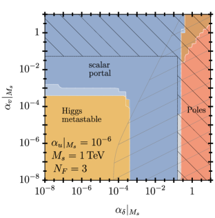
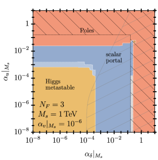
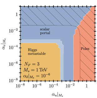
Figure 6: BSM critical surface in the $SU(N_{F})\times SU(N_{F})$ model in the $\alpha_{\delta}(M_{s})$–$\alpha_{v}(M_{s})$- (top) , $\alpha_{\delta}(M_{s})$–$\alpha_{u}(M_{s})$- (middle) and $\alpha_{u}(M_{s})$–$\alpha_{v}(M_{s})$-plane (bottom) with the remaining quartic feeble, at $10^{-6}$, and $N_{F}=3$ and $M_{s}=1\,\text{TeV}$. Same color coding as Fig. 3 with blue corresponding to the vacuum $V^{+}$.

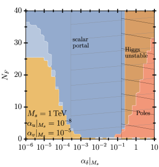
Figure 7: BSM critical surface in the $SU(N_{F})\times SU(N_{F})$ model in the $\alpha_{\delta}(M_{s})-N_{F}$ plane for $M_{s}=1\,\text{TeV}$, $\alpha_{u}(M_{s})=10^{-8}$ and $\alpha_{v}(M_{s})=10^{-5}$. Same color coding as Fig. 6.

Fig. 7 displays the interplay between $N_{F}$ of the stabilization via $\alpha_{\delta}$, with tiny $\alpha_{u,v}(M_{s})$. For larger $N_{F}$, the stability window is widened. Approximately, we find

$$\frac{1.4\cdot 10^{-3}}{N_{F}}\lesssim\,\alpha_{\delta}(M_{s})\lesssim\begin{cases}(0.05\dots 0.08)\,N_{F},\,\,N_{F}\lesssim 10\\ 0.25,\qquad\qquad\qquad N_{F}\gtrsim 10\end{cases}$$ (23)

which is largely independent of $\alpha_{u,v}(M_{s})$ and $M_{s}$ unless both quartics are sizable $\alpha_{u,v}(M_{s})=\mathcal{O}(1)$ or $M_{s}$ is close to $M_{Pl}$. Notice that the required minimal value of $\alpha_{\delta}(M_{s})$ can always be reduced by increasing $N_{F}$ and vice versa. The maximum possible value on the other hand for $N_{F}\lesssim 10$ is dictated by avoiding subplanckian Landau poles in $\alpha_{\delta}$. This changes for $N_{F}\gtrsim 10$ where we obtain roughly $\alpha_{\delta}\lesssim 0.25$ independent of $N_{F}$, as for larger values in $\alpha_{\delta}$ the Higgs potential is destabilized. This can be understood from (21). The numerically dominant terms for large $\alpha_{\delta}$ and $N_{F}$ are $N_{F}^{2}\alpha_{\delta}^{2}-4N_{F}^{2}\alpha_{\delta}^{3}$, where the first is from one- and the second from two-loop. This contribution is negative for $\alpha_{\delta}>1/4$ independent of $N_{F}$, resulting in an unstable Higgs.

Constraints from tree-level perturbative unitarity (72), displayed by the dark hatched regions, disfavor Planck safety from large $\alpha_{\Delta}\gtrsim 5\cdot 10^{-2}$. The $\alpha_{\delta}$ bound on the other hand is not really relevant as too large values of $\alpha_{\delta}$ anyway induce poles.

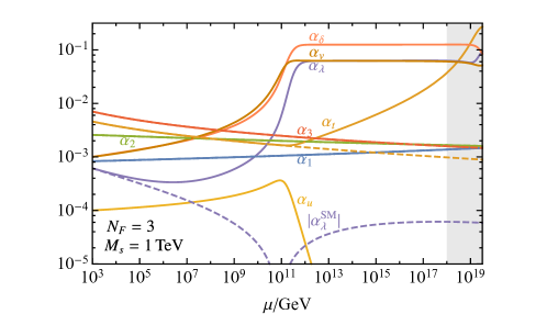
Figure 8: Two-loop renormalization group flow in the SM (dashed lines) and in the scalar $SU(N_{F})\times SU(N_{F})$ model (solid lines) for $N_{F}=3$ and $M_{s}=1\,\text{TeV}$ as well as $\alpha_{\delta,u,v}(M_{s})=(10^{-3},\,10^{-4},\,10^{-3})$. All quartic couplings are trapped in a walking regime before the Planck scale, except for $\alpha_{u}$ which asymptotically approaches zero.

Returning to the upper plot of Fig. 6, larger values of $\alpha_{v}(M_{s})$ improve the stability of the scalar potential due to the occurrence of a walking regime. In particular, the walking corresponds to the same pseudo fixed point of the $O(2N_{F}^{2})$ symmetry case. Therefore, it is expected that $\alpha_{v}$ reaches sizable values while $|\alpha_{u}|\to 0$ as the walking regime is entered, irrespective of the sign of $\alpha_{u}$, but without transitions between the vacua $V^{\pm}$ (20). This is displayed in Fig. 8. Stabilization of the Higgs within a walking regime is also possible within a range of sizable $\alpha_{u}(M_{s})$. Thus, sufficiently sizable $\alpha_{u,v}(M_{s})$ may stabilize the Higgs potential, even if $\alpha_{\delta}(M_{s})$ itself is too small to allow this, see lower plot in Fig. 6. In this case, the pure BSM quartics are driving force behind the running of $\alpha_{\delta}$ and through it the stabilization of $\alpha_{\lambda}$. In this case we roughly obtain

$$(6\dots 8)\cdot 10^{-3}\lesssim \;N_{F}^{2}\,\alpha_{v}(M_{s}),$$ (24)

$$3\cdot 10^{-3}\lesssim \;N_{F}\,\alpha_{u}(M_{s})\lesssim(6\dots 8)\cdot 10^{-2}$$ (25)

for feeble $10^{-10}\lesssim\alpha_{\delta}(M_{s})\lesssim 10^{-5}$, vanishing $\alpha_{u/v}(M_{S})$ and TeV-ish $M_{s}$. The upper bound on $\alpha_{u}(M_{s})$ is due to the occurrence of subplanckian Landau poles in $\alpha_{u}$ which constitutes an important qualitative difference to $\alpha_{v}$-induced Planck safety. When increasing $M_{s}$ by a few orders of magnitude also the lower bounds on $\alpha_{u,v}(M_{s})$ increase, as there is less RG time to rescue the potential and the effect is channeled though $\alpha_{\delta}$. This is similar to the $O(N_{S})$ model.

With increasing $N_{F}$, the window of stabilization for $\alpha_{v}(M_{s})$ is generically larger than the one for $\alpha_{u}(M_{s})$. This follows from the leading-$N_{F}$ contributions to (22), which are of order $\propto N_{F}^{2}\alpha_{v}$ and $\propto N_{F}\alpha_{u}$, respectively.

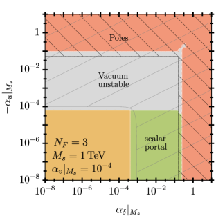
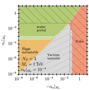
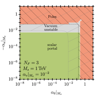
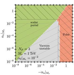
Figure 9: BSM critical surface of the $SU(N_{F})\times SU(N_{F})$ model for negative $\alpha_{u}(M_{s})$ with $M_{s}=1\,\text{TeV}$, $N_{F}=3$ in the $\alpha_{\delta}(M_{s})-\alpha_{u}(M_{s})$ plane and $\alpha_{v}(M_{s})=10^{-4}$ ($\alpha_{v}(M_{s})=10^{-2}$) in the upper (lower) plot on the left, and in the $\alpha_{u}(M_{s})-\alpha_{v}(M_{s})$ plane for $\alpha_{\delta}(M_{s})=10^{-4}$ ($\alpha_{\delta}(M_{s})=10^{-2}$) in the upper (lower) plot on the right. Dark (light) green corresponds to strict (soft) Planck safety in vacuum $V^{-}$, with other colors as in Fig. 3.

III.6 Negative BSM Quartics

Here, we investigate whether Planck safety can be realized in the $SU(N_{F})\times SU(N_{F})$ model for negative BSM quartics at the matching scale. The tree-level stability conditions (20) in principle allow all BSM quartics to be negative as long as $\alpha_{u}$ and $\alpha_{v}$ are not negative at the same time. Depending on the sign of $\alpha_{u}(\mu_{0})$ stability can be realized in the two different vacuum configurations $V^{\pm}$. Recall also that $\alpha_{u}$ is technically natural. Thus, no RG induced sign changes in $\alpha_{u}$ occur, and for negative (positive) $\alpha_{u}(\mu_{0})$ Planck safety can only be realized in $V^{-}$ ($V^{+}$). This is an important difference to models with additional Yukawa couplings Hiller:2019mou ; Hiller:2020fbu ; PlanckSafeQuark which spoil the technical naturalness of $\alpha_{u}$ and can induce transitions between the vacua.

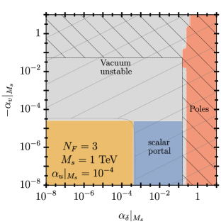
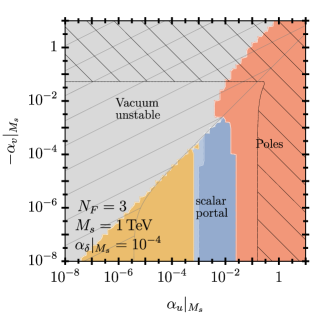
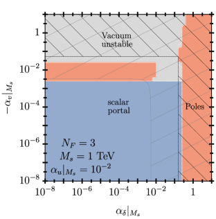
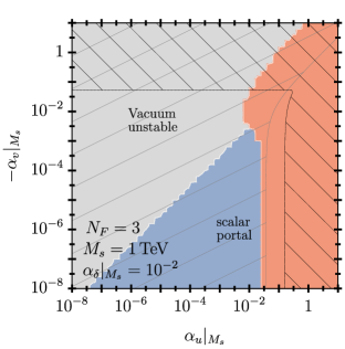
Figure 10: BSM critical surface of the $SU(N_{F})\times SU(N_{F})$ model for negative $\alpha_{v}(M_{s})$ with $M_{s}=1\,\text{TeV}$, $N_{F}=3$ in the $\alpha_{\delta}(M_{s})-\alpha_{v}(M_{s})$ plane for $\alpha_{u}(M_{s})=10^{-4}$ ($\alpha_{u}(M_{s})=10^{-2}$) in the upper (lower) plot on the left, and in the $\alpha_{u}(M_{s})-\alpha_{v}(M_{s})$ plane for $\alpha_{\delta}(M_{s})=10^{-4}$ ($\alpha_{\delta}(M_{s})=10^{-2}$) in the upper (lower) plot on the right. Same color coding as Fig. 6.

We start by analyzing a negative Higgs portal coupling. Although in principle allowed by the stability conditions (20) we find that $\alpha_{\delta}(\mu_{0})<0$ is excluded by a Planck-safe RG evolution. This result is independent of the signs of $\alpha_{u,v}(\mu_{0})$ and analogous to our findings in the $O(N_{S})$ model, discussed in Sec. III.4: also in the $SU(N_{F})\times SU(N_{F})$ model the coefficient in the one-loop beta function for the portal, $X$, is positive, see (22), for any $N_{F}\geq 1$, or otherwise inconsistent with stability (20). Therefore, with arguments analogous to the $O(N_{S})$ model, for portal couplings $\alpha_{\delta}(\mu_{0})<0$ one always encounters vacuum instabilities or poles below $M_{\text{Pl}}$.

For the pure BSM quartics $\alpha_{u,v}$, on the other hand, we find significant Planck-safe regions in parameter space for either negative $\alpha_{u}(\mu_{0})$ or $\alpha_{v}(\mu_{0})$. In general, $\alpha_{u}(\mu_{0})<0$ requires $\alpha_{v}(\mu_{0})>|\alpha_{u}(\mu_{0})|$, see (20), to realize stability in the vacuum $V^{-}$, also illustrated in Fig. 9. Likewise, $\alpha_{v}(\mu_{0})<0$ implies positive $\alpha_{u}(\mu_{0})>N_{F}|\alpha_{v}(\mu_{0})|$ to satisfy (20) in $V^{+}$, consistent with Fig. 10. Other features are similar to the previous discussion of non-negative quartics.

IV Probing the Higgs Potential

The Higgs portal coupling in combination with spontaneous symmetry breaking in the SM and BSM sector induces mixing between the SM Higgs and the BSM scalar. This directly affects the phenomenology of the 125 GeV Higgs boson. Here we discuss the constraints on the models’ parameters from the Higgs width and its couplings. In particular, we work out the impact of our models on the coupling of the Higgs boson to a pair of $Z$ bosons and on its self-couplings at leading order.

IV.1 Higgs-BSM Mixing

We discuss scalar mixing, and refer to App. C for further details. In addition to electroweak symmetry breaking, with a VEV $v_{h}$ for the Higgs as $H=\frac{1}{\sqrt{2}}(h+v_{h})$, BSM symmetry breaking may occur and the BSM scalar $S$ acquires a vacuum expectation value (VEV), $v_{s}$, as

$$O(N_{S}): \;S_{i}=(s+v_{s})\delta_{i1}+\dots,$$ (26)

$$V^{+}: \;S_{ij}=\frac{\delta_{ij}}{\sqrt{2N_{F}}}(s+v_{s}+i\,\tilde{s})+\dots$$

$$V^{-}: \;S_{ij}=\frac{\delta_{i1}\delta_{j1}}{\sqrt{2}}(s+v_{s}+i\,\tilde{s})+\dots\,.$$

with the real SM and BSM Higgs modes $h$ and $s$, respectively, as propagating degrees of freedom. Here $V^{\pm}$ refer to the different vacuum configurations in the $SU(N_{F})\times SU(N_{F})$ model. The ellipsis refer to additional components of the broken scalar fields that are irrelevant for the mixing between $s$ and $h$, while $\tilde{s}$ is an additional pseudoreal scalar singlet which appears for complex fields. Plugging (26) into the potentials (10) and (19) one obtains the scalar potential, which depends only on $h$, $s$ and the VEVs,

$$V(h,s)= -\frac{\mu_{H}^{2}}{2}(h+v_{h})^{2}-\frac{1}{2}\mu_{S}^{2}(s+v_{s})^{2}+\frac{\lambda}{4}(h+v_{h})^{4}$$ (27)

$$+\frac{\Delta}{\mathcal{N}^{2}}(s+v_{s})^{4}+\frac{\delta}{2\mathcal{N}}(h+v_{h})^{2}(s+v_{s})^{2}\,,$$

where the model-specific expressions are given for

$$O(N_{S}): \quad\mathcal{N}=1,\quad\Delta=v,$$ (28)

$$V^{+}: \quad\mathcal{N}=2,\quad\Delta=\frac{u}{N_{F}}+v,$$

$$V^{-}: \quad\mathcal{N}=2,\quad\Delta=u+v.$$

The fields $h$ and $s$ in the gauge basis mix into the mass eigenstates $h^{\prime}$ and $s^{\prime}$, (61), (62).We identify the masses of these physical fields with the Higgs mass $M_{h}=m_{h^{\prime}}=125$ GeV and the BSM scalar $M_{s}=m_{s^{\prime}}>M_{h}$. The scalar mixing angle $\beta$ can be written as

$$\tan 2\beta=\frac{\alpha_{\delta}}{\sqrt{\alpha_{\lambda}\alpha_{\Delta}}}\frac{m_{h}m_{s}}{m_{s}^{2}-m_{h}^{2}}\,,$$ (29)

and is induced by the portal coupling; $m_{h}\propto v_{h}$ and $m_{s}\propto v_{s}$ denote mass terms in the gauge basis, cf. App. C.

The five (six) a priori independent model parameters $\mu_{H}^{2},\,\mu_{S}^{2},\,\lambda,\,\delta,\,v$ (and $u$) in the potential of the $O(N_{S})$ ($SU(N_{F})\times SU(N_{F})$) model are correlated by experimental determinations of $M_{h}$ and $v_{h}\simeq 246\,\text{GeV}$ (e.g. via Fermi’s constant $G_{F}=(\sqrt{2}v_{h}^{2})^{-1}$). Hence, the models are controlled by three (four) BSM degrees of freedom, for which we choose $M_{s},\,\alpha_{\delta}(M_{s}),\,\alpha_{v}(M_{s})$ (and $\alpha_{u}(M_{s})$) in addition to the number of flavors $N_{S}$ ($N_{F}$). This implies also that the Higgs quartic coupling $\lambda(M_{s})$ becomes a function of these parameters, see (69) for the tree-level matching, and in general deviates from its SM value $\lambda_{\text{SM}}=\tfrac{M_{h}^{2}}{2v_{h}^{2}}$. While this effect can be sizable, with observable consequences worked out in Sec. IV.3, it has only a minor effect on the running, cf. Sec. II

In general, mixing reduces the decay width of the physical Higgs $h^{\prime}$ to SM final states $\{f\}$ compared to the SM by a global factor

$$\Gamma(h^{\prime}\rightarrow\{f\})=\cos^{2}\beta\;\Gamma^{\text{SM}}(h\rightarrow\{f\})\,,$$ (30)

subject to a model-independent 95% c.l. limit Dawson:2021jcl

$$|\sin\beta|\leq 0.2$$ (31)

from combined Higgs signal strength measurements from ATLAS ATLAS:2019nkf and CMS CMS:2020gsy .

IV.2 Trilinear, Quartic and $ZZh$ Higgs Couplings

The scalar mixing affects all couplings of the physical Higgs boson. In particular, $g_{h^{\prime}ZZ}$, the coupling to $Z$’s is reduced in comparison to the SM one, $g_{hZZ}^{\text{SM}}$, with relative shift

$$\delta g_{hZZ}=\frac{g_{h^{\prime}ZZ}}{g_{hZZ}^{\text{SM}}}-1=\cos\beta-1\,,$$ (32)

with the second expression holding at tree-level. The Higgs coupling to $W$’s is analogously affected by mixing, however, experimentally weaker constrained and has smaller projected sensitivity than the $Z$ FCC:2018byv , so we focus on the latter. Currently, $\delta g_{hZZ}$ is experimentally constrained at the level of 6% by ATLAS ATLAS:2022vkf and 7% by CMS CMS:2022dwd . There is also a constraint from ATLAS assuming equal coupling modifiers to pairs of $Z$ and $W$ bosons with an accuracy of 3.1% ATLAS:2022vkf , which would still result in a slightly weaker bound on $\beta$ than (31) from the Higgs signal strength. However, the projected sensitivities to $\delta g_{hZZ}$ of 1.5% at HL-LHC Cepeda:2019klc and 0.16% at FCC-ee FCC:2018byv improve the bound on $|\sin\beta|$ to 0.17 and 0.06, respectively. The ILC at 500 GeV (1 TeV) center of mass energy has a sensitivity of $0.3\%\,(0.17\%)$ in the $hZZ$ coupling ILC:2019gyn .

Our models also impact the triple self coupling $\kappa_{3}$ of the Higgs boson. The SM tree-level expression $V^{(3)}_{\text{SM}}=\lambda_{\text{SM}}v_{h}h^{3}\equiv\kappa_{3}^{\text{SM}}h^{3}$ is modified by mixing. The cubic terms in the scalar potential in the gauge basis read

$$V^{(3)}(h,s)=\lambda v_{h}h^{3}+\frac{\delta}{\mathcal{N}}v_{s}h^{2}s+\frac{\delta}{\mathcal{N}}v_{h}hs^{2}+\frac{4\Delta}{\mathcal{N}^{2}}v_{s}s^{3}$$ (33)

which after rotating to the mass basis via (62) yields

$$V^{(3)}(h^{\prime},s^{\prime})\supset \;\kappa_{3}h^{\prime 3}$$ (34)

$$= \left(\lambda v_{h}\cos^{3}\beta-\frac{\delta v_{s}}{\mathcal{N}}\cos^{2}\beta\sin\beta\right.$$

$$\left.+\frac{\delta v_{h}}{\mathcal{N}}\cos\beta\sin^{2}\beta-\frac{4\Delta v_{s}}{\mathcal{N}^{2}}\sin^{3}\beta\right)h^{\prime 3}$$

and thus

$$\frac{\kappa_{3}}{\kappa_{3}^{\text{SM}}}= \frac{\lambda}{\lambda_{\text{SM}}}\cos^{3}\beta-\frac{\delta v_{s}}{\mathcal{N}\lambda_{\text{SM}}v_{h}}\cos^{2}\beta\sin\beta$$ (35)

$$+\frac{\delta}{\mathcal{N}\lambda_{\text{SM}}}\cos\beta\sin^{2}\beta-\frac{4\Delta v_{s}}{\mathcal{N}^{2}\lambda_{\text{SM}}v_{h}}\sin^{3}\beta\,.$$

Experimentally, $\kappa_{3}$ is currently only poorly constrained by ATLAS and CMS with $-1.5<\kappa_{3}/\kappa_{3}^{\text{SM}}<6.7$ ATLAS:2021jki and $-1.24<\kappa_{3}/\kappa_{3}^{\text{SM}}<6.49$ CMS:2022dwd , respectively. Bounds are expected to significantly improve in the future with projected sensitivities of 50% at HL-LHC, 44% at FCC-ee and 5% at FCC-hh FCC:2018byv . The ILC at 500 GeV (1 TeV) center of mass energy has a sensitivity of $27\%\,(10\%)$ in the trilinear ratio (35) ILC:2019gyn .

We also consider BSM effects in the Higgs quartic self-coupling, encoded in $V^{(4)}(h^{\prime},s^{\prime})\supset\kappa_{4}h^{\prime 4}$, where in the SM $\kappa_{4}^{\text{SM}}=\tfrac{\lambda_{\text{SM}}}{4}$, and

$$\frac{\kappa_{4}}{\kappa_{4}^{\text{SM}}}\!=\!\frac{\lambda}{\lambda_{\text{SM}}}\cos^{4}\beta\!+\!\frac{2\delta}{\mathcal{N}\lambda_{\text{SM}}}\cos^{2}\beta\sin^{2}\beta\!+\!\frac{4\Delta}{\mathcal{N}^{2}\lambda_{\text{SM}}}\sin^{4}\beta\,.$$ (36)

No LHC constraints on $\kappa_{4}$ have been reported to date Workman:2022ynf . The FCC-hh has a projected sensitivity of $-4\lesssim\kappa_{4}/\kappa_{4}^{\text{SM}}\lesssim 10$ for $0\lesssim\kappa_{3}/\kappa_{3}^{\text{SM}}\lesssim 1$ FCC:2018byv . Note that unitarity provides an upper limit $\kappa_{4}/\kappa_{4}^{\text{SM}}\lesssim 65$, see App. D.

BSM effects in (32), (35), and (36) have been implemented at the leading order. An analysis of the Higgs observables in the SM and BSM beyond tree-level as well as a global higher order analysis of electroweak precision observables in the scalar singlet models such as in Dawson:2021jcl is desirable but beyond the scope of this work.

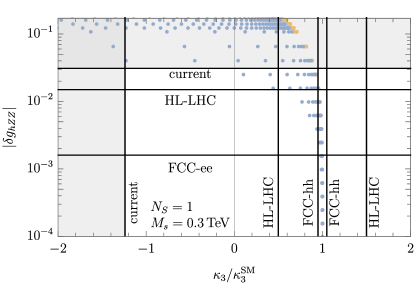
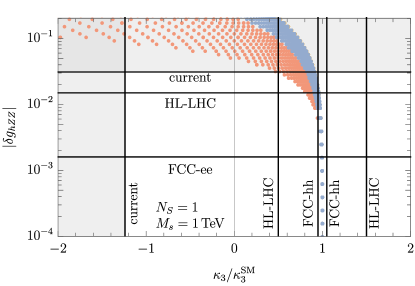
Figure 11: Higgs couplings $\delta g_{hZZ}$ (32) versus $\kappa_{3}$ (35) in the $N_{S}=1$ scalar singlet model for $M_{s}=0.3\,\text{TeV}$ (top), $M_{s}=1\,\text{TeV}$ (bottom). The scattered dots correspond to different BSM coupling values $\alpha_{\delta}|_{M_{s}}$ and $\alpha_{v}|_{M_{s}}$ as in Fig. 3. The color indicates the Planck fate, same color coding as Fig. 3, blue means safety. Black horizontal and vertical lines correspond to experimental sensitivities at current and future colliders. Gray regions are excluded by current data.

IV.3 Signatures of Safe Scalar Singlet Extensions

We begin with a few analytical approximations, which explain the main features of the phenomenology of Higgs couplings in Planck-safe scalar singlet extensions. For small mixing angles $\beta\ll 1$, one obtains

$$\beta\simeq\frac{\delta}{2\sqrt{\lambda\Delta}}\frac{m_{h}}{M_{s}}\,.$$ (37)

Expanding in small $\beta$ and using (69) we find that in the trilinear ratio (35) the $\mathcal{O}(\beta)$-term cancels against the shift in $\lambda$. Hence, the leading effect arises at $\mathcal{O}(\beta^{2})$

$$\frac{\kappa_{3}}{\kappa_{3}^{\text{SM}}}\simeq 1-\beta^{2}\left(\frac{3}{2}\frac{\lambda}{\lambda_{\text{SM}}}-\frac{\delta}{\mathcal{N}\lambda_{\text{SM}}}\right)\,.$$ (38)

For the quartic ratio (36) we obtain, using the same approximations

$$\frac{\kappa_{4}}{\kappa_{4}^{\text{SM}}}\simeq 1+\frac{\delta^{2}}{4\Delta\lambda_{\text{SM}}}\,,$$ (39)

which is unsuppressed by neither small $\beta$ nor large BSM masses. Within Planck-safe regions with $\delta\gtrsim 2\sqrt{\lambda\Delta}$, this is a positive and sizable correction of order unity to the quartic ratio, see Fig. 3 in the $O(N_{S})$ and Fig. 6 in the matrix scalar model. The BSM shift is enhanced by $M_{s}$ for fixed $\beta$, and one therefore expects $\kappa_{4}$ to be more sensitive to larger masses than $\kappa_{3}$.

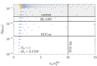
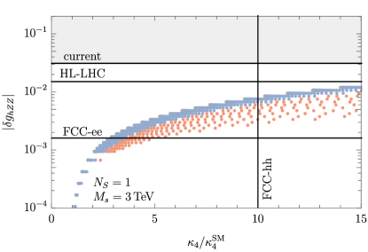
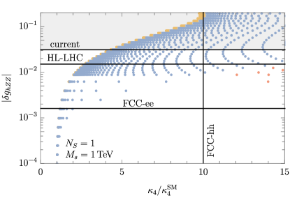
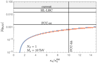
Figure 12: Higgs couplings $\delta g_{hZZ}$ (32) versus $\kappa_{4}$ (36) in the scalar singlet model $(N_{S}=1)$ for different scalar field masses, showing $M_{s}=0.3\,\text{TeV}$ (top left), $M_{s}=1\,\text{TeV}$ (bottom left), $M_{s}=3\,\text{TeV}$ (top right), and $M_{s}=10\,\text{TeV}$ (bottom right); color-coding and exclusion regions as in Fig. 11. The admissible band of Planck-safe models becomes increasingly narrower with increasing mass.

For the diboson-Higgs coupling we expect small BSM effects of the order

$$\delta g_{hZZ}\simeq-\frac{\beta^{2}}{2}\,.$$ (40)

Unlike in $\kappa_{4}$, both BSM shifts in $\kappa_{3}$ and $\delta g_{hZZ}$ are suppressed by $M_{s}^{2}$, see (37), i.e., they are smaller for larger BSM scalar masses.

In the following we validate these features in the numerical analysis, which is based on the full expressions without expansions in small mixing angles or mass ratios.

The couplings $\delta g_{hZZ}$ (32) and $\kappa_{3}$ (35), as well as $\delta g_{hZZ}$ (32) against $\kappa_{4}$ (36) in the $N_{S}=1$ scalar singlet extension are shown in Fig. 11 and Fig. 12 for $M_{s}=0.3\,\text{TeV}$ and $M_{s}=1\,\text{TeV}$. Due to its higher sensitivity to larger $M_{s}$ we also show BSM effects in $\kappa_{4}/\kappa_{4}^{\text{SM}}$ for $3\,\text{TeV}$ and $10\,\text{TeV}$. For larger $M_{s}$ the band becomes increasingly narrower and tuned, and decouples from $\delta g_{hZZ}$ and $\kappa_{3}$. Blue dots correspond to Planck-safety.

We observe that safe scalar singlet models are already probed, with some part of the parameter space ruled out by the LHC (gray area in Fig. 11 and Fig. 12). The bound on $\delta g_{hZZ}$ excludes large deviations in $\kappa_{3}/\kappa_{3}^{\text{SM}}$. In the nearer future the HL-LHC Cepeda:2019klc will improve the limit on $\delta g_{hZZ}$ by roughly a factor of two, and could observe the trilinear for smaller $M_{s}$; the projected reach in parameter space is larger with $\delta g_{hZZ}$ than with $\kappa_{3}$. For TeV-ish BSM masses and above BSM effects in $\kappa_{3}$ are within $20\%$, and within $10\%$ after the HL-LHC phase due to the correlation with $hZZ$-limits, and detectable at the future hadron collider FCC-hh FCC:2018byv . For a future FCC-ee collider FCC:2018byv one expects an order of magnitude improvement in $\delta g_{hZZ}$ from the current limit. In contrast, the enhancement of $\kappa_{4}/\kappa_{4}^{\text{SM}}$ can be sizable, typically a factor of a few, and even $O(10)$ factors are achievable. Consequently, for larger $M_{s}\approx 10\,\text{TeV}$, signatures slip out of reach of the FCC-ee due to the smallness of $\delta g_{hZZ}$. We stress that an enhanced Higgs quartic may well be the only signature of the model, which is in reach of the FCC-hh (see Fig. 12).

Changing $N_{S}$ but keeping $\alpha_{\delta},\,\alpha_{v}$ and $M_{s}$ would give identical values of $\kappa_{3}$ and $\delta g_{hZZ}$, so the plots hold generically in $O(N_{S})$ models. While for larger $N_{S}$ Planck safety can be obtained already for lower coupling values and hence, points corresponding to a metastable Higgs can convert to Planck-safe ones in Fig. 11, this does not increase to region of available, and testable parameter space.

The phenomenology of the $SU(N_{F})\times SU(N_{F})$ model in Planck-safe parameter configurations is very similar to the $O(N_{S})$ model, and therefore not shown. Note that Planck-safe parameter configurations in the vacua $V^{\pm}$ map onto similar points in the Higgs coupling space and require additional observables such as those related to the flavor structure to disentangle them.

For further phenomenological discussion of the $O(N_{S})$ model and the $SU(N_{F})\times SU(N_{F})$ model we refer to e.g. Dawson:2021jcl ; Huang:2016cjm and Hiller:2020fbu , respectively. BSM signatures include mixing induced BSM scalar decays to SM fermions or gauge bosons via the Higgs portal.

V Conclusions

We revisited the stability analysis of the SM Higgs potential with the state-of-the art precision in theory and experiment. The mass of the top quark followed by the strong coupling constant are the most critical observables to determine vacuum stability, with their correlation shown in Fig. 2. The region (green) in which the Higgs quartic remains positive is away from the PDG 2023 averages of $M_{t}$ and $\alpha_{s}$ by $-3.9\sigma$ and $+8\sigma$, respectively. Correlations matter and ideally should be provided by combined experimental determinations, such as from CMS CMS:2019esx , which finds lower central values closer to the stability region and more sizable uncertainties. An overview of shifts using different inputs for the top mass is provided in Tab. 1. We estimate that reducing uncertainties by a factor of two is sufficient to establish or refute SM vacuum stability at the $5\sigma$ level. Our results encourage further combined analyses of the top quark mass together with the strong coupling constant to shed light on the stability of the SM vacuum.

In addition, we have investigated the Higgs portal mechanism as a minimally invasive route towards stability beyond the SM. We systematically studied a variety of singlet scalar field extensions covering real, complex, vector and matrix scalar fields, with and without flavor symmetries, thereby also extending earlier works. Particular emphasis has been given to the interplay of the Higgs, portal, and BSM quartic couplings and their higher order RG evolution up to the Planck scale.

We find that a TeV-ish (but possibly much heavier) BSM scalar singlets with modest portal coupling within $10^{-3}\lesssim\alpha_{\delta}(\mu_{0})\lesssim 10^{-2}$ suffices to achieve stability. For larger mass the required value of $\alpha_{\delta}(\mu_{0})$ slowly increases as there is less RG time left to rescue the potential (Fig. 3). The value of the Higgs portal coupling can also be quite feeble by increasing the number of BSM scalars, or for sizeable pure BSM quartic couplings by indirect stabilization from RG-mixing (13), (22). Negative values of the portal $\alpha_{\delta}(\mu_{0})$ – although in principle allowed – are inconsistent with Planck safety because they run into trouble, either into subplanckian Landau poles or RG-induced vacuum instabilities. The $SU(N_{F})\times SU(N_{F})$ models, on the other hand, feature two pure BSM quartics for which we find sizeable Planck-safe areas in the parameter space with one of them negative (Fig. 9 and Fig. 10). These models can also break flavor universality spontaneously.

There is sizable room for new physics in the scalar singlet models that can be tested at the HL-LHC Cepeda:2019klc in Higgs couplings to electroweak bosons, its trilinear coupling, and for sub-TeV BSM masses (Fig. 11). A future lepton collider, such as the FCC-ee FCC:2018byv can explore these models further by reaching deeper into regions with smaller Higgs-BSM mixing due to an order of magnitude higher sensitivity to $\delta g_{hZZ}$. BSM effects in the quartic Higgs self-coupling (36), on the other hand, can experience significant enhancements by a factor of up to ten (Fig. 12), which require a future collider with sufficient energy and precision such as the FCC-hh FCC:2018byv .

The Higgs-to-electroweak-boson and the trilinear self-couplings provide promising nearer term collider observables of planck-safe flavorful scalar singlet extensions. Further studies exploring the Higgs couplings are encouraged.

Appendix A SM Effective Potential

In this appendix, we recall the main steps to find the SM effective potential following standard procedures, e.g. Ford:1992pn ; Martin:2013gka ; Martin:2014bca ; Martin:2015eia ; Martin:2017lqn ; Martin:2018emo . Classically, the stability of the Higgs potential only depends on the sign of its quartic interaction $\propto\lambda(H^{\dagger}H)^{2}$. At quantum level, additional corrections arise as the classical potential is improved to the effective potential, including quantum effects and operators of higher powers in the field.

Technically, the quantum effective potential $V_{\text{eff}}$ is obtained by expanding the Higgs $H=\frac{1}{\sqrt{2}}h+\hat{H}$ around a constant, classical field $h$ and integrating out the quantum field $\hat{H}$. The RG equation for the effective potential reads

$$0=\left(\frac{\partial}{\partial\ln\mu}+\gamma\frac{\partial}{\partial\ln h}+\sum_{i}\beta_{i}\frac{\partial}{\partial\alpha_{i}}\right)V_{\text{eff}}\,,$$ (41)

where $\gamma$ is the anomalous dimension of the classical field $h$ and $\alpha_{i}$ are all SM couplings with their beta functions $\beta_{i}$. As the classical potential is $V=\tfrac{1}{4}\lambda h^{4}$, we relate the effective potential to a dimensionless parameter $\lambda_{h}$ via

$$V_{\text{eff}}=\tfrac{1}{4}\lambda_{h}(\alpha_{i},z_{h})\,h^{4}\quad\text{ where }\quad z_{h}=h/\mu$$ (42)

without loss of generality. It follows that

$$0=\left(4\gamma+(\gamma-1)\frac{\partial}{\partial\ln z_{h}}+\sum_{i}\beta_{i}\frac{\partial}{\partial\alpha_{i}}\right)\lambda_{h}\,.$$ (43)

Next, the field dependent part $z_{h}$ is separated by the ansatz

$$\lambda_{h}(\alpha_{i},z_{h})=\left(\frac{z_{h}}{z_{0}}\right)^{4\gamma/(1-\gamma)}\lambda_{\text{0}}(\alpha_{i},z_{0})\,.$$ (44)

This ansatz corresponds to an absolutely stable potential which is positive, bounded from below and convex. The quantity $z_{0}$ is a positive parameter independent of the field $h$. Using this ansatz, only an implicit RG dependence remains in the couplings, which cancels for the effective potential

$$\sum_{i}\beta_{i}\frac{\partial}{\partial\alpha_{i}}\lambda_{h}=0\,.$$ (45)

The quantum effective potential thus reads

$$V_{\text{eff}}=\frac{1}{4}\lambda_{\text{0}}(\alpha_{i},z_{0})\,h^{4}\left(\frac{z_{h}}{z_{0}}\right)^{4\gamma/(1-\gamma)}\,.$$ (46)

The crucial property is that the field dependent factor $\propto h^{4}(z_{h}/z_{0})^{4\gamma/(1-\gamma)}$ is manifestly positive, meaning that the stability of the effective potential only hinges on the sign of $\lambda_{0}$. As the effective potential is RG invariant, neither its stability nor sign of $\lambda_{0}$ can change at a different choice of renormalization scale $\mu$. Similarly, the explicit choice of $z_{0}$ does not change the sign of $\lambda_{0}$ either, as it only amounts to a positive rescaling

$$\lambda_{0}(\alpha_{i},z_{0}^{\prime})=\lambda_{0}(\alpha_{i},z_{0})\left(\frac{z_{0}}{z_{0}^{\prime}}\right)^{4\gamma/(1-\gamma)}\,,$$ (47)

as $z_{0}$ drops out from the effective potential. Nevertheless, the parameter $z_{0}$ is crucial to optimize the numerical precision in the determination of $\lambda_{0}$. The quartic coupling $\lambda_{0}(\alpha_{i},z_{0})$ is obtained by evaluating fixed-order calculations of the effective potential Ford:1992pn ; Martin:2013gka ; Martin:2014bca ; Martin:2015eia ; Martin:2017lqn ; Martin:2018emo at constant field value $z_{h}=z_{0}$. This yields

$$\lambda_{0}= {}\lambda+\frac{1}{(4\pi)^{2}}\bigg{[}$$ (48)

$${}+4\lambda^{2}\left(\ln\frac{2\lambda}{z_{0}}-\frac{3}{2}\right)+\frac{3}{8}g_{2}^{4}\left(\ln\frac{g_{2}^{2}}{4z_{0}}-\frac{5}{6}\right)$$

$$+\frac{3}{16}(g_{1}^{2}+g_{2}^{2})^{2}\left(\ln\frac{g_{1}^{2}+g_{2}^{2}}{4z_{0}}-\frac{5}{6}\right)$$

$$-\sum_{f}N_{f}y_{f}^{4}\left(\ln\frac{y_{f}^{2}}{2z_{0}}-\frac{3}{2}\right)\bigg{]}+\mathcal{O}(\text{2 loop})\,,$$

where the last line is summed over all fermions flavors with $N_{f}$ being their respective color multiplicity. We use $z_{0}$ to minimize the size of loop corrections to $\lambda_{0}$ by controlling the size of logarithmic terms. Around the electroweak scale, the strong gauge coupling $g_{3}$ is most sizable, but only appears at two loops in $\lambda_{0}$ and outside of logarithms. The next largest coupling is the top Yukawa $y_{t}$. Therefore, logarithms stemming from top corrections are switched off by choosing $z_{0}=\tfrac{1}{2}y_{t}^{2}$. This choice has been adopted in Sec. II, together with $\alpha_{\lambda,\text{eff}}=\lambda_{0}/(4\pi)^{2}$, see (2) and (5). Notice that other logarithms in (48) become more sizable by this choice. However, these terms remain nevertheless subleading owing to the smallness of couplings in front of them.

In Sec. II, we observe cases where the coupling $\alpha_{\lambda,\text{eff}}$ turns negative under the RG evolution at very high scales, which is in tension with the ansatz (46) of an absolutely stable potential. In these cases, we cannot ascertain that the effective potential is convex and bounded from below.

Appendix B Some Terminology and Conventions

In this work, we are primarily interested in whether BSM models stabilize the SM effective potential, or continue to exhibit instabilities, or even worse Landau poles, prior to the Planck scale $M_{\text{Pl}}$. Then, possible realizations include outright stability at the Planck scale ($0\leq\alpha_{\lambda}$), SM-like meta-stability (mildly negative $\alpha^{\rm SM}_{\lambda}\leq\alpha_{\lambda}<0$), and vacuum instability ($\alpha_{\lambda}<\alpha^{\rm SM}_{\lambda}<0)$. To differentiate between scenarios, and for want of some terminology, we refer to the different possibilities as follows:

• Strict Planck Safety: We characterize BSM models as (strictly) Planck-safe, provided the tree-level potential including both SM and BSM fields is stable for all scales up to the Planck scale, $\mu_{0}\leq\mu\leq M_{\text{Pl}}$. We also demand that the RG running does not lead to Landau poles in any of the other couplings.

• Soft Planck Safety: We characterize BSM models as (softly) Planck-safe, provided their tree-level potential including both SM and BSM fields is stable at the Planck scale, but we allow $\alpha_{\lambda}$ to be negative at intermediate scales, but not more negative than in the SM,

  $$-10^{-4}\lesssim\min\alpha_{\lambda}(\mu),\quad\alpha_{\lambda}(M_{\text{Pl}})>0\,.$$ (49)

  As the stability conditions of the portal coupling $\delta$ involve $\sqrt{\lambda}$ we require

  $$\alpha_{\delta}(\mu)>0\quad\text{if}\quad-10^{-4}\lesssim\alpha_{\lambda}(\mu)\lesssim 0.$$ (50)

  in accordance with the stability conditions (11), (20) in the limit $\lambda\to 0$. We also demand that the running does not lead to Landau poles elsewhere.

• SM-like Theories: We characterize BSM models as SM-like provided the Higgs quartic remains mildly negative at the Planck scale, yet less negative as in the SM,

  $$-10^{-4}\lesssim\alpha_{\lambda}(M_{\text{Pl}})\lesssim 0\,,$$ (51)

  and without spurious Landau poles prior to $M_{\rm Pl}$.

With this classification in mind, we have adopted the following color-coding in key figures of this paper. If an RG flow features a subplanckian Landau pole it is always labeled with Pole (red). A pole-free RG flow with $\min\alpha_{\lambda}(\mu)<-10^{-4}$ is marked as Higgs unstable (brown). A RG evolution without poles and with $\min\alpha_{\lambda}(\mu)>-10^{-4}$ but violating BSM stability conditions (11), (20), or (50) is titled Vacuum unstable (gray). If BSM stability conditions in (11), (20) or (50) are fulfilled and $-10^{-4}\lesssim\min\alpha_{\lambda}(\mu)\lesssim 0$ as stated in (49) the corresponding RG flow is SM-like if $-10^{-4}<\alpha_{\lambda}(M_{\text{Pl}})\leq 0$ (yellow) or (softly) Planck safe, if $\alpha_{\lambda}(M_{\text{Pl}})>0$ (light blue). If all tree-level stability conditions (11) or (20) are fulfilled for all scales $\mu_{0}\leq\mu\leq M_{\text{Pl}}$, models are (strictly) Planck safe (dark blue). In Fig. 13, we illustrate our terminology exemplary for a SM extension with a real scalar field and various portal couplings.

Figure 13: A selection of trajectories for the Higgs quartic coupling $|\alpha_{\lambda}(\mu)|$, illustrating the main scenarios depending on the Higgs portal coupling $\alpha_{\delta}$ at the matching scale $M_{s}$, exemplarily for a model with a real BSM scalar ($M_{s}=1\,\text{TeV}$, $\alpha_{v}(M_{s})=10^{-2}$, see also (10)). For feeble $\alpha_{\delta}=10^{-8}$ (yellow, metastability), the theory remains SM-like. Mildly increasing $\alpha_{\delta}=10^{-6}$ (purple), the theory becomes (softly) Planck-safe, with $\alpha_{\lambda}$ changing sign twice prior to the Planck scale. Increasing $\alpha_{\delta}$ even further, $\alpha_{\delta}=10^{-3}$ (dark blue), the model becomes strictly Planck safe, with $\alpha_{\lambda}(\mu)>0$ up to $M_{Pl}$. For strongly coupled settings, $\alpha_{\delta}=10^{-1}$ (red), a Landau pole arises right above the matching scale, and the running cannot be continued to the Planck scale.

Appendix C Scalar Mixing

The kinetic and mass terms for a single, free scalar field $S$ read

$$\mathcal{L}_{S}=\frac{\mathcal{N}}{2}(\partial_{\mu}S)^{\dagger}\partial^{\mu}S-\frac{\mathcal{N}}{2}m_{S}^{2}S^{\dagger}S\,,$$ (52)

where $\mathcal{N}=2$ ($\mathcal{N}=1$) for a complex (real) scalar field which is canonically normalized. When spontaneous symmetry breaking in the BSM sector occurs, a VEV $v_{s}$ and a real scalar $s$ emerge via (26) along with other components which depend on details of the scalar sector. In particular, a $O(N_{S})$ symmetric BSM model additionally yields a scalar field $\phi$ in the fundamental representation of the remaining $O(N_{S}-1)$ symmetry:

$$O(N_{S}):\quad S=\begin{pmatrix}v_{s}+s\\ \phi^{1}\\ \vdots\\ \phi^{N_{S}-1}\end{pmatrix}\,.$$ (53)

As the $SU(N_{F})_{L}\times SU(N_{F})_{R}$ symmetric scalar is complex, there is also a pseudo-real singlet mode $\tilde{s}$ in the spectrum. The vacuum $V^{-}$ implies a spontaneous breaking of $SU(N_{F})_{L}\times SU(N_{F})_{R}\to SU(N_{F}-1)_{L}\times SU(N_{F}-1)_{R}$, and the additional fields $\phi_{L,R}$ appear in the fundamental of the $SU(N_{F}-1)_{L,R}$ subgroup and as singlet in the other, as well as $\Phi$ which is bifundamental

$$S=\begin{pmatrix}\frac{1}{\sqrt{2}}(v_{s}+s+i\tilde{s})\!&\!\phi_{R}^{1}\!&\!\dots\!&\!\phi_{R}^{N_{F}-1}\!\\ \phi_{L}^{1}\!&\!\Phi^{1,1}\!&\!\dots\!&\!\Phi^{1,N_{F}-1}\!\\ \vdots\!&\!\vdots\!&\!\!&\!\vdots\!\\ \phi_{L}^{N_{F}-1}\!&\!\Phi^{N_{F}-1,1}\!&\!\dots\!&\!\Phi^{N_{F}-1,N_{F}-1}\!\end{pmatrix}\,.$$ (54)

In the $V^{+}$ configuration, the chiral symmetry collapses to the vectorial part $SU(N_{F})_{L}\times SU(N_{F})_{R}\to SU(N_{F})_{V}$, giving rise to the real and pseudoreal adjoints $R$ and $I$, respectively. Thus the unbroken scalar decomposes to

$$S_{ij}=\frac{\delta_{ij}}{\sqrt{2N_{F}}}\left(v_{s}+s+i\tilde{s}\right)+\left(R^{a}+iI^{a}\right)t^{a}_{ij}\,,$$ (55)

where $t^{a}_{ij}$ are the (traceless) generators of $SU(N_{F})_{V}$. Expanding the unbroken, model-dependent scalar potentials (10) and (19) in terms of these scalar components yields lengthy expressions. Fortunately, to investigate the mixing with the SM Higgs only the modes $h$ and $s$ matter. This part of the potential can be expressed in a model-independent fashion via (27), where the specific expressions in the different models are obtained from (28).

The potential (27) is minimized for $\text{d}V(h,s)/\text{d}h=\text{d}V(h,s)/\text{d}s=0$, which yields

$$\mu_{H}^{2}=\lambda v_{h}^{2}+\frac{\delta}{\mathcal{N}}v_{s}^{2},\qquad\mu_{S}^{2}=\frac{4\Delta}{\mathcal{N}^{2}}v_{s}^{2}+\frac{\delta}{\mathcal{N}}v_{h}^{2}.$$ (56)

The quadratic terms in $V_{h,s}$ can be identified with mass terms for the real scalar fields $h$ and $s$ as

$$V(h,s)\subset+\frac{1}{2}m_{h}^{2}h^{2}+\frac{1}{2}m_{hs}^{2}hs+\frac{1}{2}m_{s}^{2}s^{2}\,,$$ (57)

$$m_{h}^{2}= \frac{\text{d}^{2}V(h,s)}{\text{d}h^{2}}|_{h=s=0}=2\lambda v_{h}^{2}\,,$$ (58)

$$m_{hs}^{2}= 2\frac{\text{d}^{2}V(h,s)}{\text{d}h\text{d}s}|_{h=s=0}=\frac{4}{\mathcal{N}}\delta v_{h}v_{s}\,,$$

$$m_{s}^{2}= \frac{\text{d}^{2}V(h,s)}{\text{d}s^{2}}|_{h=s=0}=\frac{8}{\mathcal{N}^{2}}\Delta v_{s}^{2}\,,$$

and

$$v_{h}^{2}=\frac{m_{h}^{2}}{2\lambda},\quad v_{s}^{2}=\frac{\mathcal{N}^{2}m_{s}^{2}}{8\Delta},\quad m_{hs}^{2}=\frac{\delta}{\sqrt{\lambda\Delta}}m_{h}m_{s}\,.$$ (59)

The mass terms can be compactly written in matrix form

$$M^{2}=\begin{pmatrix}m_{s}^{2}&m_{hs}^{2}/2\\ m_{hs}^{2}/2&m_{h}^{2}\end{pmatrix}=\begin{pmatrix}\frac{8}{\mathcal{N}^{2}}\Delta v_{s}^{2}&\frac{2}{\mathcal{N}}\delta v_{h}v_{s}\\ \frac{2}{\mathcal{N}}\delta v_{h}v_{s}&2\lambda v_{h}^{2}\end{pmatrix}\,.$$ (60)

The scalars $h$ and $s$ mix into mass eigenstates $h^{\prime}$ and $s^{\prime}$

$$\begin{pmatrix}s^{\prime}\\ h^{\prime}\end{pmatrix}=O\begin{pmatrix}s\\ h\end{pmatrix}$$ (61)

with the orthogonal mixing matrix $O$

$$O=\begin{pmatrix}\cos\beta&\sin\beta\\ -\sin\beta&\cos\beta\end{pmatrix}\,.$$ (62)

The mixing angle $\beta$ is readily obtained by exploiting that the (1,2) element of the diagonalized mass matrix

$$M^{\prime 2}=OM^{2}O^{T}=\begin{pmatrix}m_{s^{\prime}}^{2}&0\\ 0&m_{h^{\prime}}^{2}\end{pmatrix}$$ (63)

vanishes. This yields

$$\tan 2\beta= \frac{m^{2}_{hs}}{m_{s}^{2}-m_{h}^{2}}$$ (64)

$$= \frac{\frac{4}{\mathcal{N}}\delta v_{h}v_{s}}{\left(\frac{8}{\mathcal{N}^{2}}\Delta v_{s}^{2}-2\lambda v_{h}^{2}\right)}$$

$$= \frac{\delta}{\sqrt{\lambda\Delta}}\frac{m_{h}m_{s}}{m_{s}^{2}-m_{h}^{2}}\,,$$

cf. (29). Evaluating $M^{2}=O^{T}M^{\prime 2}O$, (63), in components yields

$$m_{s}^{2} =\cos^{2}\beta\,m_{s^{\prime}}^{2}+\sin^{2}\beta\,m_{h^{\prime}}^{2}\,,$$ (65)

$$m_{h}^{2} =\cos^{2}\beta\,m_{h^{\prime}}^{2}+\sin^{2}\beta\,m_{s^{\prime}}^{2}\,,$$ (66)

$$\sin 2\beta =\frac{m_{hs}^{2}}{m_{s^{\prime}}^{2}-m_{h^{\prime}}^{2}}\,.$$ (67)

The latter equation demonstrates that for BSM scalars heavier than the Higgs in Planck-safe models which require $\delta$ positive, hence $m^{2}_{hs}>0$, the mixing angle must be positive, too. The first two equations show that $m_{h^{\prime}}^{2}\leq m_{s}^{2},m_{h}^{2}\leq m_{s^{\prime}}^{2}$ (for the mass ordering $m_{h^{\prime}}<m_{s^{\prime}}$ which we assume), and that in the small angle approximation $0<\beta\ll 1$ the diagonal mass terms coincide, $m_{s}^{\prime}\simeq m_{s}$, $m_{h}^{\prime}\simeq m_{h}$. This approximation works well for $m_{s}^{\prime}$ but breaks down for $m_{h}^{\prime}$ once $\beta m_{s}^{\prime}\gtrsim m_{h}^{\prime}$. Note that (67) implies

$$|\delta|<4\sqrt{\lambda\Delta}\,\frac{m_{s^{\prime}}^{2}-m_{h^{\prime}}^{2}}{m_{s}m_{h}}.$$ (68)

The Higgs quartic $\lambda$ can be obtained from (66) as

$$\lambda= \frac{m_{h}^{2}}{2v_{h}^{2}}=\lambda_{\text{SM}}+\frac{\sin^{2}\beta}{2v_{h}^{2}}(m_{s^{\prime}}^{2}-m_{h^{\prime}}^{2})$$ (69)

$$\simeq \;\lambda_{\text{SM}}+\frac{\delta^{2}}{4\Delta}\left(1+\frac{m_{h^{\prime}}^{2}}{m_{s^{\prime}}^{2}}+\mathcal{O}\left(\frac{m_{h^{\prime}}^{4}}{m_{s^{\prime}}^{4}}\right)\right)\,,$$

where $\lambda_{\text{SM}}=m_{h^{\prime}}^{2}/(2v_{h}^{2})$, and in the last step we expanded in small $\beta$ (37). In the main text physical masses are denoted by

$$m_{h^{\prime}}=M_{h}=125\,\text{GeV},\qquad m_{s^{\prime}}=M_{s}\,.$$ (70)

We briefly comment on a contribution $-\mu_{det}(det(S)+det(S^{\dagger}))$ to the scalar potential (19), which is allowed by the global symmetries. For $N_{F}=3$ $\mu_{det}$ becomes a dimensionful parameter, which is negligible for the RG-analysis. On the other hand, it induces in $V^{+}$ an additional term in $V(h,s)$, $-\mu_{det}(s+v_{s})^{3}/(\sqrt{2}\sqrt{N_{F}}^{3})$, which contributes to $\kappa_{3}$ as $\mu_{det}\sin^{3}\beta/(\sqrt{2}\sqrt{N_{F}}^{3})$. As it is of third order in the mixing angle, which is small, (31), and further suppressed by $N_{F}^{3/2}$, it is negligible for the phenomenological analysis. However, $\mu_{det}$ modifies the minimization condition $\mu_{S}^{2}=\Delta v_{s}^{2}+\frac{\delta}{2}v_{h}^{2}-\frac{v_{s}\mu_{det}}{\sqrt{2N_{F}}}$, and breaks the one-to-one correspondence (58) between mass and VEV for the BSM scalar, $m_{s}^{2}=2\Delta v_{s}^{2}-\frac{v_{s}\mu_{det}}{\sqrt{2N_{F}}}$. The value of $v_{s}$ depends now on $\mu_{det}$, for a given BSM mass. While this does not affect the sign of $m^{2}_{hs}$ and therefore $\beta$, it makes the analysis of parameters more involved by adding another degree of freedom. We therefore neglect $\mu_{det}$ for the purpose of this work. In $V^{-}$ no such contribution to (27) arises.

Appendix D Unitarity Constraints

Tree-level perturbative unitarity in $2\to 2$ scattering of the physical SM and BSM Higgs modes $h$ and $s$ with a potential

$$V^{(4)}(h,s)\supset\frac{\lambda}{4}h^{4}+\frac{\Delta}{\mathcal{N}^{2}}s^{4}+\frac{\delta}{2\mathcal{N}}h^{2}s^{2}\,$$ (71)

requires Dawson:2021jcl

$$\alpha_{\lambda}\lesssim\frac{1}{6\pi},\quad\alpha_{\Delta}\lesssim\frac{\mathcal{N}^{2}}{24\pi},\quad\alpha_{\delta}\lesssim\frac{\mathcal{N}}{4\pi},\quad$$ (72)

assuming negligible scalar mixing, see App. C.

References

- (1) G. Degrassi, S. Di Vita, J. Elias-Miro, J. R. Espinosa, G. F. Giudice, G. Isidori et al., Higgs mass and vacuum stability in the Standard Model at NNLO, JHEP 08 (2012) 098 [1205.6497].
- (2) G. Hiller, T. Höhne, D. F. Litim and T. Steudtner, Portals into Higgs vacuum stability, Phys. Rev. D 106 (2022) 115004 [2207.07737].
- (3) G. Hiller, T. Höhne, D. F. Litim and T. Steudtner, Vacuum Stability as a Guide for Model Building, in 57th Rencontres de Moriond on Electroweak Interactions and Unified Theories, 5, 2023, 2305.18520.
- (4) ATLAS, CMS collaboration, Addendum to the report on the physics at the HL-LHC, and perspectives for the HE-LHC: Collection of notes from ATLAS and CMS, CERN Yellow Rep. Monogr. 7 (2019) Addendum [1902.10229].
- (5) FCC collaboration, FCC Physics Opportunities: Future Circular Collider Conceptual Design Report Volume 1, Eur. Phys. J. C 79 (2019) 474.
- (6) CEPC Study Group collaboration, CEPC Conceptual Design Report: Volume 2 - Physics & Detector, 1811.10545.
- (7) ILC collaboration, The International Linear Collider. A Global Project, 1901.09829.
- (8) M. Casarsa, D. Lucchesi and L. Sestini, Experimentation at a muon collider, 2311.03280.
- (9) Particle Data Group collaboration, Review of Particle Physics, PTEP 2022 (2022) 083C01.
- (10) CMS collaboration, Measurement of normalised multi-differential cross sections in pp collisions at TeV, and simultaneous determination of the strong coupling strength, top quark pole mass, and parton distribution functions, Eur. Phys. J. C 80 (2020) 658 [1904.05237].
- (11) D. F. Litim and T. Steudtner, ARGES – Advanced Renormalisation Group Equation Simplifier, Comput. Phys. Commun. 265 (2021) 108021 [2012.12955].
- (12) G. Hiller, C. Hormigos-Feliu, D. F. Litim and T. Steudtner, Anomalous magnetic moments from asymptotic safety, Phys. Rev. D 102 (2020) 071901 [1910.14062].
- (13) G. Hiller, C. Hormigos-Feliu, D. F. Litim and T. Steudtner, Model Building from Asymptotic Safety with Higgs and Flavor Portals, Phys. Rev. D 102 (2020) 095023 [2008.08606].
- (14) S. Bißmann, G. Hiller, C. Hormigos-Feliu and D. F. Litim, Multi-lepton signatures of vector-like leptons with flavor, Eur. Phys. J. C 81 (2021) 101 [2011.12964].
- (15) R. Bause, G. Hiller, T. Höhne, D. F. Litim and T. Steudtner, B-anomalies from flavorful U(1)′ extensions, safely, Eur. Phys. J. C 82 (2022) 42 [2109.06201].
- (16) Hiller, Höhne, Litim and Steudtner, Planck safety from Vector-like Quarks and Flavorful Scalars, (in preparation) (2024) .
- (17) D. F. Litim and F. Sannino, Asymptotic safety guaranteed, JHEP 12 (2014) 178 [1406.2337].
- (18) D. F. Litim, M. Mojaza and F. Sannino, Vacuum stability of asymptotically safe gauge-Yukawa theories, JHEP 01 (2016) 081 [1501.03061].
- (19) A. D. Bond and D. F. Litim, Theorems for Asymptotic Safety of Gauge Theories, Eur. Phys. J. C 77 (2017) 429 [1608.00519].
- (20) T. Buyukbese and D. F. Litim, Asymptotic Safety of Gauge Theories Beyond Marginal Interactions, PoS LATTICE2016 (2017) 233.
- (21) A. D. Bond and D. F. Litim, More asymptotic safety guaranteed, Phys. Rev. D 97 (2018) 085008 [1707.04217].
- (22) A. D. Bond and D. F. Litim, Asymptotic safety guaranteed in supersymmetry, Phys. Rev. Lett. 119 (2017) 211601 [1709.06953].
- (23) A. D. Bond, D. F. Litim, G. Medina Vazquez and T. Steudtner, UV conformal window for asymptotic safety, Phys. Rev. D 97 (2018) 036019 [1710.07615].
- (24) A. D. Bond, G. Hiller, K. Kowalska and D. F. Litim, Directions for model building from asymptotic safety, JHEP 08 (2017) 004 [1702.01727].
- (25) K. Kowalska, A. Bond, G. Hiller and D. Litim, Towards an asymptotically safe completion of the Standard Model, PoS EPS-HEP2017 (2017) 542.
- (26) A. D. Bond and D. F. Litim, Price of Asymptotic Safety, Phys. Rev. Lett. 122 (2019) 211601 [1801.08527].
- (27) A. D. Bond, D. F. Litim and T. Steudtner, Asymptotic safety with Majorana fermions and new large equivalences, Phys. Rev. D 101 (2020) 045006 [1911.11168].
- (28) M. Fabbrichesi, C. M. Nieto, A. Tonero and A. Ugolotti, Asymptotically safe SU(5) GUT, Phys. Rev. D 103 (2021) 095026 [2012.03987].
- (29) A. D. Bond, D. F. Litim and G. M. Vazquez, Conformal windows beyond asymptotic freedom, Phys. Rev. D 104 (2021) 105002 [2107.13020].
- (30) A. Falkowski, C. Gross and O. Lebedev, A second Higgs from the Higgs portal, JHEP 05 (2015) 057 [1502.01361].
- (31) N. Khan and S. Rakshit, Study of electroweak vacuum metastability with a singlet scalar dark matter, Phys. Rev. D 90 (2014) 113008 [1407.6015].
- (32) H. Han and S. Zheng, New Constraints on Higgs-portal Scalar Dark Matter, JHEP 12 (2015) 044 [1509.01765].
- (33) I. Garg, S. Goswami, K. N. Vishnudath and N. Khan, Electroweak vacuum stability in presence of singlet scalar dark matter in TeV scale seesaw models, Phys. Rev. D 96 (2017) 055020 [1706.08851].
- (34) E. Gabrielli, M. Heikinheimo, K. Kannike, A. Racioppi, M. Raidal and C. Spethmann, Towards Completing the Standard Model: Vacuum Stability, EWSB and Dark Matter, Phys. Rev. D 89 (2014) 015017 [1309.6632].
- (35) J. Elias-Miro, J. R. Espinosa, G. F. Giudice, H. M. Lee and A. Strumia, Stabilization of the Electroweak Vacuum by a Scalar Threshold Effect, JHEP 06 (2012) 031 [1203.0237].
- (36) M. Gonderinger, H. Lim and M. J. Ramsey-Musolf, Complex Scalar Singlet Dark Matter: Vacuum Stability and Phenomenology, Phys. Rev. D 86 (2012) 043511 [1202.1316].
- (37) R. Costa, A. P. Morais, M. O. P. Sampaio and R. Santos, Two-loop stability of a complex singlet extended Standard Model, Phys. Rev. D 92 (2015) 025024 [1411.4048].
- (38) V. V. Khoze, C. McCabe and G. Ro, Higgs vacuum stability from the dark matter portal, JHEP 08 (2014) 026 [1403.4953].
- (39) L. A. Anchordoqui, I. Antoniadis, H. Goldberg, X. Huang, D. Lust, T. R. Taylor et al., Vacuum Stability of Standard Model++, JHEP 02 (2013) 074 [1208.2821].
- (40) P. Bandyopadhyay and R. Mandal, Vacuum stability in an extended standard model with a leptoquark, Phys. Rev. D 95 (2017) 035007 [1609.03561].
- (41) P. Bandyopadhyay, S. Jangid and A. Karan, Constraining scalar doublet and triplet leptoquarks with vacuum stability and perturbativity, Eur. Phys. J. C 82 (2022) 516 [2111.03872].
- (42) N. Chakrabarty, Doubly charged scalars and vector-like leptons confronting the muon g-2 anomaly and Higgs vacuum stability, Eur. Phys. J. Plus 136 (2021) 1183 [2010.05215].
- (43) Y. Hamada, K. Kawana and K. Tsumura, Landau pole in the Standard Model with weakly interacting scalar fields, Phys. Lett. B 747 (2015) 238 [1505.01721].
- (44) A. Latosinski, A. Lewandowski, K. A. Meissner and H. Nicolai, Conformal Standard Model with an extended scalar sector, JHEP 10 (2015) 170 [1507.01755].
- (45) M.-L. Xiao and J.-H. Yu, Stabilizing electroweak vacuum in a vectorlike fermion model, Phys. Rev. D 90 (2014) 014007 [1404.0681].
- (46) M. Dhuria and G. Goswami, Perturbativity, vacuum stability, and inflation in the light of 750 GeV diphoton excess, Phys. Rev. D 94 (2016) 055009 [1512.06782].
- (47) A. Salvio and A. Mazumdar, Higgs Stability and the 750 GeV Diphoton Excess, Phys. Lett. B 755 (2016) 469 [1512.08184].
- (48) M. Son and A. Urbano, A new scalar resonance at 750 GeV: Towards a proof of concept in favor of strongly interacting theories, JHEP 05 (2016) 181 [1512.08307].
- (49) A. Dutta Banik, A. K. Saha and A. Sil, Scalar assisted singlet doublet fermion dark matter model and electroweak vacuum stability, Phys. Rev. D 98 (2018) 075013 [1806.08080].
- (50) D. Borah, R. Roshan and A. Sil, Sub-TeV singlet scalar dark matter and electroweak vacuum stability with vectorlike fermions, Phys. Rev. D 102 (2020) 075034 [2007.14904].
- (51) D. Chowdhury and O. Eberhardt, Global fits of the two-loop renormalized Two-Higgs-Doublet model with soft Z2 breaking, JHEP 11 (2015) 052 [1503.08216].
- (52) N. Khan and S. Rakshit, Constraints on inert dark matter from the metastability of the electroweak vacuum, Phys. Rev. D 92 (2015) 055006 [1503.03085].
- (53) P. Ferreira, H. E. Haber and E. Santos, Preserving the validity of the Two-Higgs Doublet Model up to the Planck scale, Phys. Rev. D 92 (2015) 033003 [1505.04001].
- (54) P. M. Ferreira and B. Swiezewska, One-loop contributions to neutral minima in the inert doublet model, JHEP 04 (2016) 099 [1511.02879].
- (55) S. Bhattacharya, P. Ghosh, A. K. Saha and A. Sil, Two component dark matter with inert Higgs doublet: neutrino mass, high scale validity and collider searches, JHEP 03 (2020) 090 [1905.12583].
- (56) B. Swiezewska, Inert scalars and vacuum metastability around the electroweak scale, JHEP 07 (2015) 118 [1503.07078].
- (57) N. Chakrabarty and B. Mukhopadhyaya, High-scale validity of a two Higgs doublet scenario: metastability included, Eur. Phys. J. C 77 (2017) 153 [1603.05883].
- (58) P. Schuh, Vacuum Stability of Asymptotically Safe Two Higgs Doublet Models, Eur. Phys. J. C 79 (2019) 909 [1810.07664].
- (59) E. Bagnaschi, F. Brümmer, W. Buchmüller, A. Voigt and G. Weiglein, Vacuum stability and supersymmetry at high scales with two Higgs doublets, JHEP 03 (2016) 158 [1512.07761].
- (60) ATLAS collaboration, Observation of a new particle in the search for the Standard Model Higgs boson with the ATLAS detector at the LHC, Phys. Lett. B 716 (2012) 1 [1207.7214].
- (61) CMS collaboration, Observation of a New Boson at a Mass of 125 GeV with the CMS Experiment at the LHC, Phys. Lett. B 716 (2012) 30 [1207.7235].
- (62) D. Buttazzo, G. Degrassi, P. P. Giardino, G. F. Giudice, F. Sala, A. Salvio et al., Investigating the near-criticality of the Higgs boson, JHEP 12 (2013) 089 [1307.3536].
- (63) S. Alekhin, A. Djouadi and S. Moch, The top quark and Higgs boson masses and the stability of the electroweak vacuum, Phys. Lett. B 716 (2012) 214 [1207.0980].
- (64) A. Andreassen, W. Frost and M. D. Schwartz, Consistent Use of the Standard Model Effective Potential, Phys. Rev. Lett. 113 (2014) 241801 [1408.0292].
- (65) A. V. Bednyakov, B. A. Kniehl, A. F. Pikelner and O. L. Veretin, Stability of the Electroweak Vacuum: Gauge Independence and Advanced Precision, Phys. Rev. Lett. 115 (2015) 201802 [1507.08833].
- (66) S. Chigusa, T. Moroi and Y. Shoji, Decay Rate of Electroweak Vacuum in the Standard Model and Beyond, Phys. Rev. D 97 (2018) 116012 [1803.03902].
- (67) Z. Alam and S. P. Martin, Standard model at 200 GeV, Phys. Rev. D 107 (2023) 013010 [2211.08576].
- (68) S. P. Martin and D. G. Robertson, Standard model parameters in the tadpole-free pure scheme, Phys. Rev. D 100 (2019) 073004 [1907.02500].
- (69) P. A. Baikov, K. G. Chetyrkin, J. H. Kuhn and J. Rittinger, Vector Correlator in Massless QCD at Order and the QED beta-function at Five Loop, JHEP 07 (2012) 017 [1206.1284].
- (70) P. A. Baikov, K. G. Chetyrkin and J. H. Kühn, Five-Loop Running of the QCD coupling constant, Phys. Rev. Lett. 118 (2017) 082002 [1606.08659].
- (71) F. Herzog, B. Ruijl, T. Ueda, J. A. M. Vermaseren and A. Vogt, The five-loop beta function of Yang-Mills theory with fermions, JHEP 02 (2017) 090 [1701.01404].
- (72) T. Luthe, A. Maier, P. Marquard and Y. Schroder, The five-loop Beta function for a general gauge group and anomalous dimensions beyond Feynman gauge, JHEP 10 (2017) 166 [1709.07718].
- (73) K. G. Chetyrkin, G. Falcioni, F. Herzog and J. A. M. Vermaseren, Five-loop renormalisation of QCD in covariant gauges, JHEP 10 (2017) 179 [1709.08541].
- (74) K. Melnikov and T. v. Ritbergen, The Three loop relation between the MS-bar and the pole quark masses, Phys. Lett. B 482 (2000) 99 [hep-ph/9912391].
- (75) S. P. Martin, Matching relations for decoupling in the Standard Model at two loops and beyond, Phys. Rev. D 99 (2019) 033007 [1812.04100].
- (76) S. P. Martin and D. G. Robertson, Higgs boson mass in the Standard Model at two-loop order and beyond, Phys. Rev. D 90 (2014) 073010 [1407.4336].
- (77) S. P. Martin, -Boson Pole Mass at Two-Loop Order in the Pure Scheme, Phys. Rev. D 92 (2015) 014026 [1505.04833].
- (78) S. P. Martin, Top-quark pole mass in the tadpole-free scheme, Phys. Rev. D 93 (2016) 094017 [1604.01134].
- (79) S. P. Martin, Three-loop QCD corrections to the electroweak boson masses, Phys. Rev. D 106 (2022) 013007 [2203.05042].
- (80) C. Ford, I. Jack and D. R. T. Jones, The Standard model effective potential at two loops, Nucl. Phys. B 387 (1992) 373 [hep-ph/0111190].
- (81) S. P. Martin, Three-Loop Standard Model Effective Potential at Leading Order in Strong and Top Yukawa Couplings, Phys. Rev. D 89 (2014) 013003 [1310.7553].
- (82) S. P. Martin, Taming the Goldstone contributions to the effective potential, Phys. Rev. D 90 (2014) 016013 [1406.2355].
- (83) S. P. Martin, Four-Loop Standard Model Effective Potential at Leading Order in QCD, Phys. Rev. D 92 (2015) 054029 [1508.00912].
- (84) S. P. Martin, Effective potential at three loops, Phys. Rev. D 96 (2017) 096005 [1709.02397].
- (85) S. P. Martin and H. H. Patel, Two-loop effective potential for generalized gauge fixing, Phys. Rev. D 98 (2018) 076008 [1808.07615].
- (86) J. Davies, F. Herren, C. Poole, M. Steinhauser and A. E. Thomsen, Gauge Coupling Functions to Four-Loop Order in the Standard Model, Phys. Rev. Lett. 124 (2020) 071803 [1912.07624].
- (87) J. Davies, F. Herren and A. E. Thomsen, General gauge-Yukawa-quartic -functions at 4-3-2-loop order, JHEP 01 (2022) 051 [2110.05496].
- (88) A. Bednyakov and A. Pikelner, Four-Loop Gauge and Three-Loop Yukawa Beta Functions in a General Renormalizable Theory, Phys. Rev. Lett. 127 (2021) 041801 [2105.09918].
- (89) A. V. Bednyakov, A. F. Pikelner and V. N. Velizhanin, Yukawa coupling beta-functions in the Standard Model at three loops, Phys. Lett. B 722 (2013) 336 [1212.6829].
- (90) K. G. Chetyrkin and M. F. Zoller, -function for the Higgs self-interaction in the Standard Model at three-loop level, JHEP 04 (2013) 091 [1303.2890].
- (91) A. V. Bednyakov, A. F. Pikelner and V. N. Velizhanin, Three-loop SM beta-functions for matrix Yukawa couplings, Phys. Lett. B 737 (2014) 129 [1406.7171].
- (92) K. G. Chetyrkin and M. F. Zoller, Leading QCD-induced four-loop contributions to the -function of the Higgs self-coupling in the SM and vacuum stability, JHEP 06 (2016) 175 [1604.00853].
- (93) A. H. Hoang, What is the Top Quark Mass?, Ann. Rev. Nucl. Part. Sci. 70 (2020) 225 [2004.12915].
- (94) B. Dehnadi, A. H. Hoang, O. L. Jin and V. Mateu, Top Quark Mass Calibration for Monte Carlo Event Generators – An Update, 2309.00547.
- (95) R. H. Parker, C. Yu, W. Zhong, B. Estey and H. Müller, Measurement of the fine-structure constant as a test of the Standard Model, Science 360 (2018) 191 [1812.04130].
- (96) L. Morel, Z. Yao, P. Cladé and S. Guellati-Khélifa, Determination of the fine-structure constant with an accuracy of 81 parts per trillion, Nature 588 (2020) 61.
- (97) M. E. Machacek and M. T. Vaughn, Two Loop Renormalization Group Equations in a General Quantum Field Theory. 3. Scalar Quartic Couplings, Nucl. Phys. B 249 (1985) 70.
- (98) S. Dawson, P. P. Giardino and S. Homiller, Uncovering the High Scale Higgs Singlet Model, Phys. Rev. D 103 (2021) 075016 [2102.02823].
- (99) Belle-II collaboration, Evidence for Decays, 2311.14647.
- (100) R. Bause, H. Gisbert and G. Hiller, Implications of an enhanced branching ratio, Phys. Rev. D 109 (2024) 015006 [2309.00075].
- (101) ATLAS collaboration, Combined measurements of Higgs boson production and decay using up to fb-1 of proton-proton collision data at 13 TeV collected with the ATLAS experiment, Phys. Rev. D 101 (2020) 012002 [1909.02845].
- (102) CMS collaboration, Combined Higgs boson production and decay measurements with up to 137 fb-1 of proton-proton collision data at = 13 TeV, .
- (103) ATLAS collaboration, A detailed map of Higgs boson interactions by the ATLAS experiment ten years after the discovery, Nature 607 (2022) 52 [2207.00092].
- (104) CMS collaboration, A portrait of the Higgs boson by the CMS experiment ten years after the discovery., Nature 607 (2022) 60 [2207.00043].
- (105) M. Cepeda et al., Report from Working Group 2: Higgs Physics at the HL-LHC and HE-LHC, CERN Yellow Rep. Monogr. 7 (2019) 221 [1902.00134].
- (106) ATLAS collaboration, Search for Higgs boson pair production in the two bottom quarks plus two photons final state in collisions at TeV with the ATLAS detector, .
- (107) P. Huang, A. J. Long and L.-T. Wang, Probing the Electroweak Phase Transition with Higgs Factories and Gravitational Waves, Phys. Rev. D 94 (2016) 075008 [1608.06619].