Sample Relationships through the Lens of Learning Dynamics with Label InformationFewer Data → Better Generalisation: Sample Relationship from Learning Dynamics Matters

Abstract

Although much research has been done on proposing new models or loss functions to improve the generalisation of artificial neural networks (ANNs), less attention has been directed to the data, which is also an important factor for training ANNsimpact of the training data on generalisation. In this work, we start from approximating the interaction between two samples, i.e. how learning one sample would modify the model’s prediction on the other sampleother samples. Through analysing the terms involved in weight updates in supervised learning, we find that the signs of labels influence the interactions interaction between samples. Therefore, we propose the labelled pseudo Neural Tangent Kernel (lpNTK) which takes label information into consideration when measuring the interactions between samples. We first prove that lpNTK would asymptotically converge to the well-known empirical Neural Tangent Kernel asymptotically converges to the empirical neural tangent kernel in terms of the Frobenius norm under certain assumptions. Secondly, we illustrate how lpNTK helps to understand learning phenomena identified in previous work, specifically the learning difficulty of samples and forgetting events during learning. Moreover, we also show that lpNTK using lpNTK to identify and remove poisoning training samples can help to improve the generalisation performance of ANNs in image classification tasks, compared with the original whole training sets.

1 Introduction

In the past decade, artificial neural networks (ANNs) have achieved great successes with the help of large models and very large datasets (silver2016mastering; krizhevsky2017imagenet; vaswani2017attention). There are usually three components involved in training an ANN: 1) the model, i.e. the ANN itself; 2) a loss function; and 3) a dataset, usually labelled for supervised learning. Previous work has shown that generalisation performance can be boosted by i) changing the model architecture, e.g. ResNet (he2016resnet) and ViT (dosovitskiy2020vit); or ii) introducing new loss functions, e.g. focal loss (lin2017focal) and regularisation (goodfellow2016deep). Researchers have also explored methods that allow models to choose data, e.g. active learning (settles2012active), to improve the generalisation performance and reduce laborious data annotation. In this work, we focus on selecting data in order to achieve greater better generalisation performance.

Although the samples in datasets training samples are usually assumed to be independent and identically distributed (i.i.d, goodfellow2016deep), ANNs do not learn them independently: the samples independently, as the parameter update on one labelled sample will influence the predictions for many other samples. This dependency is a double-edged sword. On the plus side, the dependency between seen and unseen samples makes it possible for ANNs to output reliable predictions on held-out data (koh2017understanding). However, dependencies between samples can also cause catastrophic forgetting  (Kirkpatrick2017Forgetting), i.e. updates on a sample appearing later might erase the correct predictions for previous samples. While researchers have proposed statistics to describe such forgetting events (e.g. toneva2018forgetting; paul2021datadiet), it is an open question to identify the causes of such events. We Hence, we argue that it is necessary to investigate the relationships between samples in order to understand how data selection affects the learningand further , and further how to improve generalisation performance through manipulating data.

We first decompose the learning dynamics of ANN models in classification tasks, and show that the interactions between training samples can be well-captured by combining the empirical neural tangent kernel (eNTK NTK) with label information. Inspired by the pseudo NTK (pNTK) proposed by mohamadi2022pntk which can represent the relationship between two input samples using one scalar, we propose the labelled pseudo NTK (lpNTK) to measure the interactions between samples, i.e. how the update on one sample influences the predictions on others. As shown in Section 2.3, our lpNTK can be viewed as a linear kernel on a feature space representing each sample as a vector derived from the lpNTK. Since the angles between inner product of high-dimensional vectors can be obtusepositive/rightnegative/acutezero, we point out that there are three types of relationships between two a pair of samples: interchangeable, unrelated, and contradictory. Through Following the analysis of inner products between lpNTK representations, we find that a sample is considered as redundant if its largest inner product is not with itself, i.e. it can be removed without reducing the trained ANNs’ generalisation performance. Moreover, through experiments, we verify that two concepts from previous work can be connected to and explained by the above three types of relationships: 1) the the learning difficulty of data discussed by paul2021datadiet, and the forgetting events during ANN learning found by toneva2018forgetting; 2) the learning difficulty of data discussed by paul2021datadiet. Inspired . Furthermore, inspired by the discussion about the connections between learning difficulty and generalisation from sorscher2022beyond, we show that the generalisation performance of trained ANNs can be improved by removing part of the samples in the largest cluster obtained through farthest point clustering (FPC) with lpNTK as the similarity metric, compared with the whole original dataset. .

In summary, we make three contributions in this work: 1) we introduce a new kernel, lpNTK, which can take label information into account for ANNs to measure the interaction between sample samples during learning; 2) we provide a unified view to explain the learning difficulty of samples and forgetting events using the three types of relationships defined under lpNTK; 3) we show that generalisation performance in classification problems can be improved by carefully removing part of the samples data items that have similar lpNTK feature representations.

2 lpNTK: Interactions between Samples Sample Interaction via First-Order Taylor Approximation

In this section, we first show the first-order Taylor approximation to the interactions between two samples in a typical supervised learning task, classification. We then show how labels modify those interactions, which inspires our lpNTK. At the end of this section, we formalise our lpNTK and mathematically prove that it asymptotically converges to eNTK (NTK).

2.1 Derivation on Supervised Learning for Classification Problems

Suppose in a $K$-way classification problem, the dataset ${\mathcal{D}}$ consists of $N$ labelled samples, i.e. ${\mathcal{D}}=\{\{{\bm{x}}_{1},y_{1}\},\dots,\{{\bm{x}}_{N},y_{N}\}\}$. Our neural network model is $f({\bm{x}};{\bm{w}})\triangleq{\bm{q}}({\bm{x}})=\mathrm{softmax}({\bm{z}}({\bm{x}};{\bm{w}}))$ where ${\bm{w}}\in{\mathbb{R}}^{d}$ is the vectorised parameters, ${\bm{z}}\in\mathbb{R}^{K}$, and ${\bm{q}}\in\Delta^{K}$. To update parameters, we use the cross-entropy loss function, i.e. $L(y,{\bm{q}}({\bm{x}}))=-\log{\bm{q}}_{y}({\bm{x}})$ where ${\bm{q}}_{k}$ represents the $k$-th element of the prediction vector ${\bm{q}}$, and the back-propagation algorithm (rumelhart1986learning). At time $t$, suppose we take a step of stochastic gradient descent (SGD) with learning rate $\eta$ on a sample ${\color[rgb]{0,0,1}{\bm{x}}_{u}}$, we show that this will modify the prediction on ${\color[rgb]{1,.5,0}{\bm{x}}_{o}}\neq{\color[rgb]{0,0,1}{\bm{x}}_{u}}$ as:

$$\Delta_{{\color[rgb]{0,0,1}{\bm{x}}_{u}}}{\bm{q}}({\color[rgb]{1,.5,0}{\bm{x}}_{o}})\triangleq{\bm{q}}^{t+1}({\color[rgb]{1,.5,0}{\bm{x}}_{o}})-{\bm{q}}^{t}({\color[rgb]{1,.5,0}{\bm{x}}_{o}})\approx\eta\cdot\underbrace{{\bm{A}}^{t}({\color[rgb]{1,.5,0}{\bm{x}}_{o}})\cdot}_{K\times K}\underbrace{{\bm{K}}^{t}({\color[rgb]{1,.5,0}{\bm{x}}_{o}},{\color[rgb]{0,0,1}{\bm{x}}_{u}})}_{K\times K}\cdot\underbrace{\left({\bm{p}}_{\text{tar}}({\color[rgb]{0,0,1}{\bm{x}}_{u}})-{\bm{q}}^{t}({\color[rgb]{0,0,1}{\bm{x}}_{u}})\right)}_{K\times 1}$$ (1)

where ${\bm{A}}^{t}({\color[rgb]{1,.5,0}{\bm{x}}_{o}})\triangleq\nabla_{{\bm{z}}}{\bm{q}}^{t}({\color[rgb]{1,.5,0}{\bm{x}}_{o}})|_{{\bm{z}}^{t}}$, ${\bm{K}}^{t}({\color[rgb]{1,.5,0}{\bm{x}}_{o}},{\color[rgb]{0,0,1}{\bm{x}}_{u}})\triangleq\nabla_{{\bm{w}}}{\bm{z}}^{t}({\color[rgb]{1,.5,0}{\bm{x}}_{o}})|_{{\bm{w}}^{t}}\cdot\left(\nabla_{{\bm{w}}}{\bm{z}}^{t}({\color[rgb]{0,0,1}{\bm{x}}_{u}})|_{{\bm{w}}^{t}}\right)^{\mathsf{T}}$, and ${\bm{p}}_{\text{tar}}({\color[rgb]{0,0,1}{\bm{x}}_{u}})$ is a one-hot vector where only the ${\color[rgb]{0,0,1}y_{u}}$-th element is $1$. The full derivation is given in Appendix A.

${\bm{K}}^{t}({\color[rgb]{1,.5,0}{\bm{x}}_{o}},{\color[rgb]{0,0,1}{\bm{x}}_{u}})$ in Equation 1 is a dot product between the gradient matrix on ${\color[rgb]{0,0,1}{\bm{x}}_{u}}$ ($\nabla_{{\bm{w}}}{\bm{z}}^{t}({\color[rgb]{0,0,1}{\bm{x}}_{u}})|_{{\bm{w}}^{t}}$) and ${\color[rgb]{1,.5,0}{\bm{x}}_{o}}$ ($\nabla_{{\bm{w}}}{\bm{z}}^{t}({\color[rgb]{1,.5,0}{\bm{x}}_{o}})|_{{\bm{w}}^{t}}$). Thus, an entry $K^{t}_{ij}>0$ means that the two gradient vectors, $\nabla_{{\bm{w}};i,\cdot}{\bm{z}}^{t}({\color[rgb]{0,0,1}{\bm{x}}_{u}})$ and $\nabla_{{\bm{w}};j,\cdot}{\bm{z}}^{t}({\color[rgb]{1,.5,0}{\bm{x}}_{o}})$, are pointing in similar directions, thus learning one leads to better prediction on the other; when $K^{t}_{ij}<0$ the two gradients are pointing in opposite directions, thus learning one leads to worse prediction on the other. Regarding the case where $K^{t}_{ij}\approx 0$, the two gradient vectors are approximately orthogonal, and learning one of them has almost no influence on the other. Since ${\bm{K}}^{t}({\color[rgb]{1,.5,0}{\bm{x}}_{o}},{\color[rgb]{0,0,1}{\bm{x}}_{u}})$ is the only term that involves both ${\color[rgb]{0,0,1}{\bm{x}}_{u}}$ and ${\color[rgb]{1,.5,0}{\bm{x}}_{o}}$ at the same time, we argue that the matrix itself or a transformation of it can be seen as a similarity measure between ${\color[rgb]{0,0,1}{\bm{x}}_{u}}$ and ${\color[rgb]{1,.5,0}{\bm{x}}_{o}}$, which naturally follows from the first-order Taylor approximation. ${\bm{K}}^{t}({\color[rgb]{1,.5,0}{\bm{x}}_{o}},{\color[rgb]{0,0,1}{\bm{x}}_{u}})$ is also known as the eNTK (NTK) in vector output form.

Though ${\bm{K}}^{t}({\color[rgb]{1,.5,0}{\bm{x}}_{o}},{\color[rgb]{0,0,1}{\bm{x}}_{u}})$ is a natural similarity measure between ${\color[rgb]{1,.5,0}{\bm{x}}_{o}}$ and ${\color[rgb]{0,0,1}{\bm{x}}_{u}}$, there are two problems. First, it depends on both the samples and parameters ${\bm{w}}^{t}$, thus becomes variable over training since ${\bm{w}}^{t}$ varies over $t$. Therefore, to make this similarity metric more accurate, it is reasonable to prefer the parameters that perform the best on the validation set, i.e. parameters having the best generalisation performance. Without loss of generality, we denote such parameters as ${\bm{w}}$ in the following, and the matrix as ${\bm{K}}$. The second problem is that we can compute ${\bm{K}}({\bm{x}},{\bm{x}}^{\prime})$ for every pair of samples $({\bm{x}},{\bm{x}}^{\prime})$, but need to convert them to scalars $\kappa({\bm{x}},{\bm{x}}^{\prime})$ in order to use them as a conventional scalar-valued kernel. This also makes it possible to directly compare two similarity matrices, e.g. ${\bm{K}}$ and ${\bm{K}}^{\prime}$. It is intuitive to use $L_{p,q}$ or Frobenius norm of matrices to convert ${\bm{K}}({\bm{x}},{\bm{x}}^{\prime})$ to scalars. However, through experiments, we found that the off-diagonal entries in ${\bm{K}}^{t}({\color[rgb]{1,.5,0}{\bm{x}}_{o}},{\color[rgb]{0,0,1}{\bm{x}}_{u}})$ are usually non-zero and there are many negative entries, thus neither $L_{p,q}$-norm nor F-norm is appropriate. Instead, the findings from mohamadi2022pntk suggests that the sum of all elements in ${\bm{K}}({\bm{x}},{\bm{x}}^{\prime})$ divided by $K$ serves as a good candidate for this proxy scalar value, and they refer to this quantity as pNTK. We follow their idea, but show that the signs of elements in ${\bm{K}}$ should be considered in order to have higher test accuracy in practice. We provide empirical evidence that this is the case in Section 4.

2.2 Information From Labels

Beyond the similarity matrix ${\bm{K}}$, there are two other terms in Equation 1, the $\mathrm{softmax}$ derivative term ${\bm{A}}$ and the prediction error term ${\bm{p}}_{\text{tar}}({\color[rgb]{0,0,1}{\bm{x}}_{u}})-{\bm{q}}^{t}({\color[rgb]{0,0,1}{\bm{x}}_{u}})$. As shown in Equation 6 from Appendix A, the signs in ${\bm{A}}$ are constant across all samples. Thus, it is not necessary to take ${\bm{A}}$ into consideration when we measure the similarity between two specific samples.

Let’s now have a look at We now consider the prediction error term. In common practice, ${\bm{p}}_{\text{tar}}({\bm{x}})$ is usually a one-hot vector in which only the $y$-th element is $1$ and all others are $0$. Since ${\bm{q}}=\mathrm{softmax}({\bm{z}})\in\Delta^{K}$, we can do the following analysis of the signs of elements in the prediction error term:

$${\bm{p}}_{\text{tar}}({\color[rgb]{0,0,1}{\bm{x}}_{u}})-{\bm{q}}({\color[rgb]{0,0,1}{\bm{x}}_{u}}) =\begin{bmatrix}0-q_{1}<0\\ \dots\\ 1-q_{y}>0\\ \dots\\ 0-q_{K}<0\end{bmatrix}\Rightarrow {\bm{s}}({\color[rgb]{0,0,1}y_{u}})\triangleq\operatorname{sign}\left({\bm{p}}_{\text{tar}}({\color[rgb]{0,0,1}{\bm{x}}_{u}})-{\bm{q}}({\color[rgb]{0,0,1}{\bm{x}}_{u}})\right) =\begin{bmatrix}-1\\ \dots\\ +1\\ \dots\\ -1\end{bmatrix}.$$ (2)

The above analysis shows how learning ${\color[rgb]{0,0,1}{\bm{x}}_{u}}$ would modify the predictions on ${\color[rgb]{1,.5,0}{\bm{x}}_{o}}$, i.e. $\Delta_{{\color[rgb]{0,0,1}{\bm{x}}_{u}}}{\bm{q}}({\color[rgb]{1,.5,0}{\bm{x}}_{o}})$. Conversely, we can also approximate $\Delta_{{\color[rgb]{1,.5,0}{\bm{x}}_{o}}}{\bm{q}}({\color[rgb]{0,0,1}{\bm{x}}_{u}})$ in the same way. In this case, it is easy to see that ${\bm{K}}({\color[rgb]{0,0,1}{\bm{x}}_{u}},{\color[rgb]{1,.5,0}{\bm{x}}_{o}})={\bm{K}}({\color[rgb]{1,.5,0}{\bm{x}}_{o}},{\color[rgb]{0,0,1}{\bm{x}}_{u}})^{\mathsf{T}}$ and all elements of ${\bm{p}}_{\text{tar}}({\color[rgb]{1,.5,0}{\bm{x}}_{o}})-{\bm{q}}({\color[rgb]{1,.5,0}{\bm{x}}_{o}})$ are negative except the ${\color[rgb]{1,.5,0}y_{o}}$-th digit, since ${\bm{K}}({\color[rgb]{0,0,1}{\bm{x}}_{u}},{\color[rgb]{1,.5,0}{\bm{x}}_{o}})\cdot\left({\bm{p}}_{\text{tar}}({\color[rgb]{1,.5,0}{\bm{x}}_{o}})-{\bm{q}}({\color[rgb]{1,.5,0}{\bm{x}}_{o}})\right)={\bm{K}}({\color[rgb]{1,.5,0}{\bm{x}}_{o}},{\color[rgb]{0,0,1}{\bm{x}}_{u}})^{\mathsf{T}}\cdot\left({\bm{p}}_{\text{tar}}({\color[rgb]{1,.5,0}{\bm{x}}_{o}})-{\bm{q}}({\color[rgb]{1,.5,0}{\bm{x}}_{o}})\right)$. Therefore, for a pair of samples ${\color[rgb]{1,.5,0}{\bm{x}}_{o}}$ and ${\color[rgb]{0,0,1}{\bm{x}}_{u}}$, their labels would change the signs of the rows and columns of the similarity matrix ${\bm{K}}({\color[rgb]{1,.5,0}{\bm{x}}_{o}},{\color[rgb]{0,0,1}{\bm{x}}_{u}})$, respectively.

Note that we do not use the whole term ${\bm{p}}_{\text{tar}}({\bm{x}})-{\bm{q}}({\bm{x}})$ but only the signs of the its entries. As illustrated in Section 3.1 below, if a large fraction of samples in the dataset share similar gradients, all their prediction errors would become tiny after a relatively short period of training. In this case, taking the magnitude of ${\bm{p}}_{\text{tar}}({\bm{x}})-{\bm{q}}({\bm{x}})$ ${\bm{p}}_{\text{tar}}({\bm{x}})-{\bm{q}}({\bm{x}})(\approx\bm{0})$ into consideration leads to a conclusion that those samples are less similar dissimilar to each other because the model can accurately fit them. Therefore, we argue that the magnitudes of prediction errors are misleading for measuring the similarity between samples . from the learning dynamic perspective.

2.3 Labelled Pseudo Neural Tangent Kernel (lpNTK)

Following the analysis in Section 2.2, we introduce the following lpNTK:

$$\text{lpNTK}(({\color[rgb]{1,.5,0}{\bm{x}}_{o}},{\color[rgb]{1,.5,0}y_{o}}),({\color[rgb]{0,0,1}{\bm{x}}_{u}},{\color[rgb]{0,0,1}y_{u}})) \triangleq\frac{1}{K}\sum\left[{\bm{s}}({\color[rgb]{0,0,1}y_{u}})\cdot{\bm{s}}({\color[rgb]{1,.5,0}y_{o}})^{\mathsf{T}}\right]\odot{\bm{K}}({\color[rgb]{1,.5,0}{\bm{x}}_{o}},{\color[rgb]{0,0,1}{\bm{x}}_{u}})$$ (3)

$$=\underbrace{\left[\frac{1}{\sqrt{K}}{\bm{s}}({\color[rgb]{1,.5,0}y_{o}})^{\mathsf{T}}\nabla_{{\bm{w}}}{\bm{z}}({\color[rgb]{1,.5,0}{\bm{x}}_{o}})\right]}_{1\times d}\cdot\underbrace{\left[\nabla_{{\bm{w}}}{\bm{z}}({\color[rgb]{0,0,1}{\bm{x}}_{u}})^{\mathsf{T}}{\bm{s}}({\color[rgb]{0,0,1}y_{u}})\frac{1}{\sqrt{K}}\right]}_{d\times 1}$$

where $\odot$ denotes that element-wise product between two matrices, and ${\bm{s}}(\cdot)$ is defined in Equation 2.

The first line of Equation 3 is to emphasise the difference between our lpNTK and pNTK, i.e. we sum up the element-wise products between $\frac{1}{K}{\bm{s}}({\color[rgb]{0,0,1}y_{u}})\cdot{\bm{s}}({\color[rgb]{1,.5,0}y_{o}})^{\mathsf{T}}$ and ${\bm{K}}$. Equivalently, the second line shows that our kernel can also be thought of as a linear kernel on the feature space where a sample ${\bm{x}}$ along with its label $y$ is represented as $\frac{1}{\sqrt{K}}{\bm{s}}(y)^{\mathsf{T}}\nabla_{{\bm{w}}}{\bm{z}}({\bm{x}})$. The second expression also shows the novelty of our lpNTK, i.e. the label information is taken into the feature representations of samples.

We first verify that the lpNTK kernel matrix approximates the corresponding eNTK. Following mohamadi2022pntk, we also study the asymptotic convergence of lpNTK in terms of the Frobenius norm.

Theorem 1.

(Informal). Suppose the last layer of our neural network ${\bm{z}}({\bm{x}};{\bm{w}})$ is a linear layer of width $w$. Let $\kappa(({\bm{x}},y),({\bm{x}}^{\prime},y^{\prime}))$ be the corresponding lpNTK, and $\tilde{{\bm{K}}}({\bm{x}},{\bm{x}}^{\prime})$ be the corresponding eNTK. When the final linear layer of ${\bm{z}}({\bm{x}};{\bm{w}})$ is properly initialised, with high probability, the following holds:

$$||\frac{1}{\sqrt{w}}\kappa\left(({\bm{x}},y),({\bm{x}}^{\prime},y^{\prime})\right)\otimes{\bm{I}}_{K}-\frac{1}{\sqrt{w}}\tilde{{\bm{K}}}({\bm{x}},{\bm{x}}^{\prime})||_{F}\in{\mathcal{O}}(w^{-\frac{1}{2}})\vspace{-0.4cm}$$ (4)

where ${\bm{I}}_{K}$ is a $K$-by-by-$K$ identity matrix. A formal statement and proof of Theorem 4 are given in Appendix B.

In the following sections, we first show the connection between our lpNTK and learning phenomena discussed by toneva2018forgetting and paul2021datadiet. Then, we empirically show that our lpNTK improves the generalisation performance in a typical supervised learning task, image classification, compared to the pNTK.

3 Rethinking Easy/Hard Samples following lpNTK

Since each labelled sample $({\bm{x}},y)$ corresponds to a vector $\frac{1}{\sqrt{K}}{\bm{s}}(y)^{\mathsf{T}}\nabla_{{\bm{w}}}{\bm{z}}({\bm{x}})\in{\mathbb{R}}^{d}$ under lpNTK, and the angle angles between any two such vectors could be obtuseacute, right, or acute, obtuse, it is straightforward to see the following three types of relationships between two labelled samples:

• interchangeable samples (where the angle between samples is acute) update the parameters of the model in similar directions, thus updates on one sample make the predictions on other interchangeable samples learning one sample makes the prediction on the other sample also more accurate;

• unrelated samples which (where the angle is right) update parameters in (almost) orthogonal directions, thus updates on one sample would not modify the predictions on other sampleslearning one sample (almost) doesn’t modify the prediction on the other sample;

• contradictory samples which (where the angle is obtuse) update parameters in opposite directions, thus updates on one sample would make the predictions on the contradictory samples learning one sample makes the prediction on the other sample worse.

More details about the above three types of relationships can be found in Appendix C. In the remainder of this section, we illustrate how the above three types of relationships provide a new unified view of some existing learning phenomena, specifically easy/hard samples discussed by paul2021datadiet and forgetting events found by toneva2018forgetting.

3.1 A Unified View for Easy/Hard Samples and Forgetting Events

Suppose at time-step $t$ of training, we use a batch of data ${\mathbb{B}}^{t}=\{({\bm{x}}^{t}_{i},y^{t}_{i})\}_{i=1}^{|{\mathbb{B}}^{t}|}$ to update the parameters. Let’s We now consider how this update would influence the predictions of samples in ${\mathbb{B}}^{t-1}$ and ${\mathbb{B}}^{t+1}$. As shown by Equation 1, for a sample ${\bm{x}}^{\prime}$ in either ${\mathbb{B}}^{t-1}$ or ${\mathbb{B}}^{t+1}$, the change of its prediction is approximately $\eta\cdot{\bm{A}}^{t}({\bm{x}}^{\prime})\cdot\sum_{{\bm{x}}^{t}\in{\mathbb{B}}^{t}}{\bm{K}}^{t}({\bm{x}}^{\prime},{\bm{x}}^{t})\cdot\left({\bm{p}}_{\text{tar}}({\bm{x}}^{t})-{\bm{q}}^{t}({\bm{x}}^{t})\right)$. Note that the sum on ${\mathbb{B}}^{t}$ is still linear, as all elements in Equation 1 are linear.

Following the above analysis, it is straightforward to see that if a sample in ${\mathbb{B}}^{t-1}$ is contradictory to most of the samples in ${\mathbb{B}}^{t}$, it would most likely be forgotten, as the updates from ${\mathbb{B}}^{t}$ modify its prediction in the “wrong” direction. Furthermore, if the probability of sampling data contradictory to $({\bm{x}},y)$ is high across the training, then $({\bm{x}},y)$ would become hard to learn as the updates from this sample are likely to be cancelled out by the updates from the contradictory samples until the prediction error on the contradictory samples are low.

On the other hand, if a sample in ${\mathbb{B}}^{t+1}$ is interchangeable with most of the samples in ${\mathbb{B}}^{t}$, it would be an easy sample, as the updates from ${\mathbb{B}}^{t}$ already modified its prediction in the “correct” direction. Moreover, if there is a large group of samples that are interchangeable with each other, they will be easier to learn since the updates from all of them modify their predictions in similar directions.

Therefore, we argue that the easy/hard samples as well as the forgetting events are closely related to the interactions between the lpNTK feature representations, i.e. $\frac{1}{\sqrt{K}}{\bm{s}}(y)^{\mathsf{T}}\nabla_{{\bm{w}}}{\bm{z}}({\bm{x}})$, of the samples in a dataset. The number of interchangeable/contradictory samples can be thought as the “learning weights” of their corresponding lpNTK feature representations.

An example of and further details about the above analysis are given in Appendix D.1.

3.2 Experiment 1: Control Learning Difficultyof Samples on Smaller Datasets

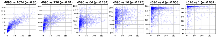
Figure 1: Correlation between the learning difficulty of each sample (red, blue, green, and orange are class 1, 2, 3, and 4, respectively) samples trained with on subsets of varying sizes. For each subfigure, the x-value is the difficulty of samples trained in on the full batch universal set (2000$4096$), while y-axis is the corresponding difficulty trained on the contrast setting (1000$1024$, 500$256$, etc.). Smaller $\rho$ (the Pearson correlation coefficient ) $\rho$ means less correlation between x and y values. The title of each panel is the settings we compare, e.g. “2000 4096 vs 1” means that we plot the learning difficulty of the same sample in on the single-batch universal set (of size $2,000$$4096$) case against the sample’s its learnability in a dataset containing just itself.

The first experiment we run is to verify that the learning difficulty of samples is mainly due to the interactions between them, rather than inherent properties of individual samples. To do so, we control the number of samples used for training models.The following experiment shows empirically verify the following two predictions derived from our explanation given in Section 3.1:

1. for a given universal set of training samples ${\mathbb{T}}$, if a subset of it $\tilde{{\mathbb{T}}}$ contains fewer samples, then the interactions in $\tilde{{\mathbb{T}}}$ is weaker compared to the interactions in ${\mathbb{T}}$, thus the learning difficulty of samples on $\tilde{{\mathbb{T}}}$ is less correlated with its learning difficulty on ${\mathbb{T}}$;

2. for a given training sample, if the other samples in the training set are more interchangeable to it, then it is easier to learn.

To verify Prediction 1, we show that the learning difficulty of a sample on the whole universal dataset ${\mathbb{T}}$ becomes less correlated with its learning difficulty on subsets of ${\mathbb{T}}$ of smaller sizes.

Following the definition from c-score and zigzag, we define the learning difficulty of a sample $({\bm{x}},y)$ as the integration between of its training loss and iterationsover epochs, or formally $\sum_{t}l({\bm{x}},y)$ where $t$ indicates the index of training epochs. In this way, larger values indicate slower convergence, and greater learning difficulty.

We run our experiments using a simple 3-layer MLP experiment using the ResNet-18 model (he2016resnet) and a subset of MNIST: we take the first $4$ classes of MNIST and select $500$ the CIFAR-10 dataset (krizhevsky2009cifar): we select $4096$ samples randomly from eachall the ten classes, giving a set of $2,000$ $40960$ samples in total.

We On this dataset, we first track the learning difficulty of samples on the whole dataset through a single training run of the model. Then, we randomly split the whole dataset into $\frac{2000}{X}$ subsets where $X\in\{1,5,10,40,200,1000\}$it into $\frac{4096}{X}$ subsets where $X\in\{1,4,16,256,1024\}$, and train a model on each of these subsets. For example, when $X=1$, we train $2,000$ $4096$ models of the same architecture and initial parameters on the $2,000$ $4096$ subsets containing just $1$ sample per class. In all experimentsruns, we use the same hyperparameters and train the network using full-batch gradient descentwith the same batch size. The results are shown in Figure 1. To eliminate the effects from hyperparameters, we also run the same experiment with varying settings of hyperparameters on both CIFAR10 (with ResNet-18, and MNIST where we train a LeNet-5 model (lecun1989handwritten). Note that we train ResNet-18 on CIFAR10 and LeNet-5 on MNIST in all the following experiments. Further details can be found in Appendix D.2.

Given our analysis in Section 3.1, we expect that the interactions between samples will be weaker more different to the universal set when the dataset size is smaller, and in the extreme case where $X=1$, the as a result the learning difficulty of the samples is purely decided by the inherent difficulty of that samplesamples would change more. As shown in Figure 1, the correlation between the learning difficulty on the whole dataset and the subsets indeed become becomes less when the subset is of smaller size, which matches with our analysis above. prediction.

To verify Prediction 2, we follow an analysis in Section 3.1, i.e. if there is a large group of samples that are interchangeable/contradictory to a sample, it should become easier/harder to learn respectively. To do so, we first need to group the labelled samples. Considering that the number of sample are usually tens of thousands and the time for computing a $\kappa({\bm{x}},{\bm{x}}^{\prime})$ is quadratic to the number of parameters, we choose the farthest point clustering (FPC) algorithm proposed by gonzalez1985clustering, since: 1) in theory, it can be sped up to ${\mathcal{O}}(N\log M)$ where $M$ is the number of centroids (feder1988optimal); 2) we cannot arbitrarily interpolate between two gradients. More details are given in Appendix D.5.

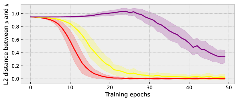
(a) MNIST

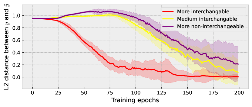
(b) CIFAR-10

Figure 2: Learning difficulty of target samples, i.e. centroids of FPC clusters, depending on whether additional samples in the same training set are interchangeable (red line), non-interchangeable (purple line), or medium interchangeable (yellow line).

As shown in the Appendix D.5, the clusters from FPC are distributed in a heavy long-tail fashion, i.e. most of the samples are in the largest cluster. A straightforward prediction following our method is that the centroid of the head cluster becomes easier due to the large number of interchangeable samples in the cluster. To verify this, we single out the centroids of all classes on MNIST and CIFAR10, and manually add an equal number of the following three types of samples: 1) most interchangeable samples from the head cluster which should make them easier; 2) most non-interchangeable samples from tail clusters which make them harder; 3) medium interchangeable samples from the “edge” of the head cluster which should have an intermediate effect on learnability. We then track the learning difficulty of the centroids on these three types of datasets over 100 random seeds, and the results are shown in Figure 2. It can be seen that the learning difficulty of the target samples become significantly lower when there are more interchangeable samples in the training set, as the red lines are always the lowest. Conversely, as the purple lines are always the highest, the learning difficulty of targets become significantly lower when there exist more non-interchangeable samples in the training set. Similarly, if the samples are medium interchangeable to the centroids, their learning difficulty is just between the other two cases. This shows that we can control the learning difficulty of a sample through controlling the relationships of other samples in the same dataset to it, which supports our Prediction 2 and further our analysis in Section 3.1. More details can be found in Appendix D.3.

3.3 Experiment 2: Predict Forgetting Events with eNTKlpNTK

The second experiments experiment we run is to check whether the forgetting events can be accurately predicted with eNTK. predicted with lpNTK ($\kappa$). However, due to that the sum operation in Equation 3 is irreversible, we propose a variant of lpNTK $\tilde{\kappa}$ to predict the forgetting events in more accuracy, of which more details are illustrated in Appendix D.4. Following toneva2018forgetting, we say a sample is forgotten at epoch $t+1$ if the model can correctly predict it at $t$ but then makes the wrong prediction at $t+1$. Given that the time for computing ${\bm{K}}({\bm{x}},{\bm{x}}^{\prime})$ is quadratic in the number of parameters, we choose benchmarks that are not too large and models that are not too over-parameterised: we train a LeNet-5 model (lecun1989handwritten) on the MNIST dataset (lecun1998gradient) and a ResNet-18 model (he2016resnet) on the CIFAR-10 dataset (krizhevsky2009cifar), both using learning rate $5\times 10^{-4}$; we use a small To guarantee the accuracy of the first-order Taylor approximation, we set learning rate to guarantee the accuracy of first-order Taylor approximation$10^{-3}$ in this experiment. In order to sample forgetting events, we track the predictions on $10$ batches of $128$ samples over $30$ iterations in the middle $10$ random seeds in the first $50$ and $700$ iterations of the training process on MNIST and CIFAR10 respectively, and observed more than $5,000$ forgetting events $7873$ and $2799$ forgetting events respectively. The results of predicting these forgetting events by eNTK a variant of lpNTK are given in Table 3.3.

As can be seen from Table 3.3, eNTK can accurately our variant of lpNTK can predict forgetting events significantly better than random guess during the training of models on both benchmark datasetsMNIST and CIFAR10. The prediction metrics on CIFAR-10 are higher, perhaps possibly because the number of parameters of ResNet-18 is greater than LeNet-5, thus the change of each parameter is smaller during a single iteration, which further leads to a more accurate Taylor approximation.

Benchmarks							Precision	Recall	F1-score
	Mean	Std	Mean	Std	Mean	Std
MNIST	$95.56\%$$42.72\%$	$\pm 8.14\%$$\pm 6.55\%$	$86.67\%$$59.02\%$	$\pm 13.67\%$$\pm 7.49\%$	$89.96\%$$49.54\%$	$\pm 7.10\%$ $\pm 6.99\%$
CIFAR-10	$96.99\%$$49.47\%$	$\pm 3.99\%$$\pm 7.06\%$	$98.99\%$$69.50\%$	$\pm 1.61\%$$\pm 7.49\%$	$97.87\%$$57.76\%$	$\pm 2.08\%$ $\pm 7.36\%$

Table 1: Performance of predicting forgetting events with our lpNTK on MNIST and CIFAR-10.

3.4 Experiment 3: Farthest Point Clustering with lpNTK to Understand Sample Learning

As mentioned in Section 3.1, if there is a large group of samples that are interchangeable with each other, all of them should become easy to learn. To verify this point, we first need to group the labelled samples. Considering that the number of sample are usually tens of thousands and the time for computing a ${\bm{K}}({\bm{x}},{\bm{x}}^{\prime})$ is quadratic to the number of parameters, we choose the farthest point clustering (FPC) algorithm proposed by gonzalez1985clustering, since: 1) in theory, it can be sped up to ${\mathcal{O}}(N\log M)$ where $M$ is the number of centroids (feder1988optimal); 2) we cannot arbitrarily interpolate between two gradients. As for the number of centroids in FPC, we use $10\%\times N$ here, as our purpose is to show that the distributions over the sizes of clusters on both MNIST and CIFAR-10 are heavily long-tailed, i.e. there are a small number of large clusters and many small clusters. The details on how we do FPC with lpNTK are given in Appendix D.5.

Through experiments, we find that most of the samples are actually in the head cluster, i.e. the largest cluster. There are a further $5-20$ clusters containing more than one sample, then the remaining clusters all contain just a single sample. This indicates that the samples in the head cluster are more interchangeable with each other than with the samples in the tail clusters. Therefore, the samples in the head clusters should be easier to learn than those in the tail clusters. To verify whether samples in larger clusters are easier, we first rank the samples in MNIST and CIFAR-10 by their learning difficulty defined as above. Among the Top-$10\%\times N$ easiest samples in MNIST and CIFAR-10, $72\%$ and $80\%$ of them are in the largest cluster. Note that the learning difficulty is averaged across random seeds, whereas the clusters are obtained with the seed that leads to the optimal validation performance. Our results suggest that samples in the largest clusters are indeed easier to learn than those in smaller clusters.

4 Use Case: Supervised Learning for Image Classification

Inspired by the finding from sorscher2022beyond that selective data pruning can lead to substantially better performance than random selection, we also explore if whether pruning samples following the clustering results under lpNTK could help to improve generalisation performance in a typical supervised learning task, image classification. In the experiments below, we use the same models and benchmarks as in Section 3.3.

4.1 Improving Improve Generalisation with lpNTK

Following the clustering analysis from Section LABEL:ssec:rethinking:fpcAppendix D.5, suppose we compose the lpNTK feature representations of samples from a cluster into a single vector. The size of the cluster can then be thought as the weight for that vector during learning. Given the cluster size distribution is heavily long-tailed, the learning would be biased towards the samples in the head cluster. However, we also know that the samples in the head cluster are more interchangeable with each other, i.e. they update parameters to in similar directions. Therefore, we ask the following two questions:

2. do Do we really need all those interchangeable samples for good generalisation?

3. can Can we improve the generalisation performance by removing the bias in the data towards the numerous interchangeable samples?

4.2 Experimental Results on Removing Remove Redundant Samples with lpNTK

To answer the first question, we define the a sample as redundant samples under lpNTK under lpNTK if the most interchangeable sample to it is not itself. Formally, for a sample ${\bm{x}}$, if there exists another sample ${\bm{x}}^{\prime}\neq{\bm{x}}$ such that $\text{lpNTK}(({\bm{x}},y),({\bm{x}}^{\prime},y^{\prime}))>\text{lpNTK}(({\bm{x}},y),({\bm{x}},y))$, then ${\bm{x}}$ is considered as a redundant sample. To verify that redundant samples identified in this way are indeed redundant and note not required for accurate generalisation, we removed them from both MNIST and CIFAR-10 , and compared the test accuracy of the models trained with or without those redundant samples. We to get de-redundant versions of them under lpNTK. To show the necessity of taking the label information into consideration, we also define redundant samples under pNTK in a similar way, i.e. for a sample ${\bm{x}}$, if there exists another sample ${\bm{x}}^{\prime}\neq{\bm{x}}$ such that $\text{pNTK}({\bm{x}},{\bm{x}}^{\prime})>\text{pNTK}({\bm{x}},{\bm{x}})$, then ${\bm{x}}$ is considered as a redundant sample under pNTK. Following this definition, we can also get de-redundant MNIST and CIFAR10 with pNTK. The test accuracy over training epochs on the whole training sets of MNIST and CIFAR-10 along with the de-redundant versions of them are shown in Table 2. To eliminate the effects from hyperparameters, we ran this experiment with over $10$ different random seeds. Note that Moreover, we did not fine-tune any hyperparameters, to make sure that the comparison between different instances of datasets are fair. ThusAs a result, the average test accuracy we obtained is not as high as reported in some other works, e.g. guo2022deepcore.

The test accuracy over training epochs on the whole training sets of MNIST and CIFAR-10 along with the de-redundant versions are shown in Figure LABEL:fig:image:redundant_exp:redundant. As shown in both plots,

Benchmarks	Full		De-redundant by pNTK		De-redundant by lpNTK
	Mean	Std	Mean	Std	Mean	Std
MNIST	99.31%	0.03%	99.27%	0.05%	99.30%	0.03%
CIFAR10	93.28%	0.06%	90.93%	0.29%	93.17%	0.23%

Table 2: Test accuracy over training epochs of models trained with MNIST and CIFAR-10 as well as the de-redundant versions. The results are averaged across $10$ different runs, and the corresponding standard deviation is also given. This table shows that removing the redundant samples defined with our lpNTK leads to a generalisation performance w.o. statistically significant difference to the whole set, while pNTK leads to worse performance.

It can be seen in Table 2 that removing the redundant samples under lpNTK leads to almost the same generalisation performance on both MNIST and CIFAR-10 (converged test accuracy obtained with the whole training sets is not significantly higher than accuracy obtained using the de-redundant version using lpNTK: on MNIST, $t(19)=0.293,p=0.774$; on CIFARCIFAR10, $t(19)=1.562,p=0.153$), whereas the de-redundant versions obtained by pNTK leads to significantly worse generalisation performance (on MNIST, $t(19)=13.718,p\ll 0.01$; on CIFARCIFAR10, $t(19)=26.252,p\ll 0.01$).

MNIST  CIFAR-10 Test accuracy over training epochs of models trained with MNIST and CIFAR-10 as well as the de-redundant versions. The lines are averaged across $10$ different runs, and the shadow areas show the corresponding standard deviation. The plots show that removing the redundant samples defined with our lpNTK leads to a generalisation performance w.o. statistically significant difference to the whole set, while pNTK leads to worse performance.

Overall, our results suggest that it is not necessary to train on multiple redundant samples (as identified using lpNTK) in order to have a good generalisation performance; the fact that identifying redundant samples using pNTK does lead to a reduction in performance shows that taking the label information into account in evaluating the relationships between samples (as we do in lpNTK) indeed leads to a better similarity measure than pNTK in practice.

4.3 Experimental Results on Debiasing DatasetsDebias Training Sets with lpNTK and FPC

To answer our second question in Section 4.1, we find i.e. whether the generalisation performance can be improved by removing part of the training data, we found several relevant clues from existing work. feldman2020longtail demonstrated that memorising the noisy or anomalous labels of the long-tailed samples is necessary in order to achieve close-to-optimal generalisation performance. paul2021datadiet and sorscher2022beyond pointed out that keeping the hardest samples can lead to better generalisation performance than keeping only the easy samples. Particularly, the results in Figure 1 of paul2021datadiet show that removing $10\%$ or $20\%$ of the easy samples can lead to better test accuracy than training on the full training set.

As discussed in Section 3, both the long-tail clusters and hard samples can be connected to the three types of relationships under our lpNTK. Specifically, samples in the head cluster are more interchangeable with each other, and thus easier to learn, while the samples in the tail clusters are more unrelated or even contradictory to samples in the head cluster and thus harder to learn. Furthermore, labels of the samples in the tail clusters are more likely to be noisy or anomalous, e.g. the “6” shown in the seventh row in Figure 13 look more like “4” than a typical “6”.

Inspired by the connections between clustering results under lpNTK and the above previous works, we: 1) remove the redundant samples from MNIST and CIFAR-10 the dataset under lpNTK; 2) cluster the remaining samples with FPC and lpNTK; 3) randomly prune $10\%$ of the samples in the largest cluster; 4) compare the test accuracy of models trained with the original datasets and the pruned versions. This sequence of steps involves removing roughly $20\%$ of the total dataset. The results are given in Figure LABEL:fig:image:poisoning_exp:improveTable 3.

Benchmarks	Full	lpNTK	EL2N	GraNd	Forgot Score
MNIST	$99.31(\pm 0.03)$%	$99.37(\pm 0.04)$%	$99.33(\pm 0.06)$%	$99.28(\pm 0.05)$%	$99.26(\pm 0.06)$%
CIFAR10	$93.28(\pm 0.06)$%	$93.55(\pm 0.12)$%	$93.32(\pm 0.07)$%	$92.87(\pm 0.13)$%	$92.64(\pm 0.22)$%

Table 3: Test accuracy of models trained with full training set and various subsets from MNIST and CIFAR10. The results are averaged across 10 different runs, and the standard deviation are also given. The table shows that randomly removing $10\%$ of the samples in the head cluster leads to better generalisation performance than the original datasets.

CIFAR-10 Test accuracy over training epochs of models trained with MNIST and CIFAR-10 as well as the pruned versions. The lines are averaged across $10$ different runs, and the shadow areas show the corresponding standard deviation. The plots show that randomly removing $10\%$ of the samples in the head cluster leads to better generalisation performance than the original datasets.

As we can see in Figure LABEL:fig:image:poisoning_exp:improveTable 3, the pruned datasets by lpNTK actually lead to higher test accuracy than the original training sets of MNIST and CIFAR-10: a $t$-test comparing converged test accuracy after training on the full vs pruned data sets lpNTK-pruned datasets shows significantly higher performance in the pruned sets (MNIST: $t(19)=-3.205,p=0.005$; CIFAR: $t(19)=-3.996,p=0.003$). This suggest suggests that it is possible to improve the generalisation performance on test sets by removing some interchangeable samples in the head cluster from FPC on lpNTK.

4.4 Discussion

Although the results illustrated above answer the two questions in Section 4.1, our experiments involve decisions on several additional parameters that merit further discussion.

In Section 4.3, we removed around $20\%$ of the total dataset, and obtained better test accuracy than after training on the full training set. However, the choice to prune this fraction is purely heuristic, and there is no theoretical guarantee for this choice. More interestingly, since lpNTK can measure any pair of annotated samples, it is also possible to use lpNTK to measure the similarity between the training and test data. So, it is intuitive to see that the interactions between training and test samples would also influence the fraction of pruned samples. As this is related to wider research topics, e.g. transfer learning, we leave this point to future work.

We also needed to specify the number of clusters as a hyperparameter for FPC. It is possible to use clustering algorithms like hierarchical clustering (HC) to get rid of this hyperparameter. However, we found that on both MNIST and CIFAR-10, HC generates heavily imbalanced binary trees, i.e. the samples are organised almost as linked lists, which makes it hard to find the boundaries between the obtained clusters. The problem of FPC, on the other hand, is that the optimal choice of $M$ is also related to both the training and test datasets and needs to be further studied. Since we focus on the effectiveness of lpNTK in this work, we leave the study about clustering on lpNTK to the future work.

5 Related WorkWorks

In this section, we discuss the connections between our work and other work from various disciplines.

[Transmission Bottleneck in Iterated Learning] This work originated as an exploration of the possible forms of transmission bottleneck in the iterated learning framework (kirby2002emergence; smith2003iterated; kirby2014iterated) on deep learning models. In existing works (e.g. guo2019emergence; lu2020countering; Ren2020Compositional; vani2021iterated; rajeswar2022multi), the transmission bottleneck is usually implemented as a limit on the number of pre-training epochs for the new generation of agents. However, as shown in human experiments by smith2003complexkirby2008cumulative, the transmission bottleneck can also be a subset of the whole training set, which works well for human agents. So, inspired by the original work on humans, we explore the possibility of using subset-sampling as a form of transmission bottleneck. As shown in Section 4.3, it is indeed possible to have higher generalisation performance through limiting the size of subsets. Thus, we argue that this work sheds the light on a new form of transmission bottleneck of iterated learning for DL agents.

[Neural Tangent Kernel] The NTK was first proposed by NTK, and was derived on fully connected neural networks, or equivalently multi-layer perceptrons. lee2019wide; yang2019tensor; yang2020tensor; yang2021tensor then extend NTK to most of the popular neural network architectures. Beyond the theoretical insights, NTK has also been applied to various kinds of DL tasks, e.g. 1) park2020towards and chen2021vision in neural architecture search; 2) zhou2021meta in meta learning; and 3) holzmuller2022framework and wang2021deep in active learning. NTK has also been applied in dataset distillation (nguyen2020dataset; nguyen2021dataset), which is closely related to our work, thus we discuss it separately in the next subsection. mohamadi2022pntk explore how to convert the matrix-valued eNTK for classification problems to scalar values. They show that the sum of the eNTK matrix would asymptotically converge to the eNTK, which inspires lpNTK. However, we emphasise the information from labels, and focus more on practical use cases of lpNTK. We also connect lpNTK with the practical learning phenomena like learning difficulty of samples and forgetting events.

[Coreset Selection and Dataset Distillation] As discussed in Section 4, we improve the generalisation performance through removing part of the samples in the training sets. This technique is also a common practice in coreset selections (CS, guo2022deepcore), although the aim of CS is usually to select a subset of training samples that can obtain generalisation performance similar to the whole set. On the other hand, we aim to show that it is possible to improve the generalisation performance via removing samples. In the meantime, as shown in Equation 3, our lpNTK is defined on the gradients of the outputs w.r.t the parameters. Work on both coreset selection (killamsetty2021grad) and dataset distillation (zhao2021grad) have also explored the information from gradients for either selecting or synthesising samples. However, these works aimed to match the gradients of the loss function loss function w.r.t the parameter on the selected/synthesised samples with the whole dataset, whereas we focus on the gradients between samples in the training set.

6 Conclusion

In this work, we start from studied the impact of data relationships on generalisation by approximating the interactions between labelled samples, i.e. how learning one sample modifies the prediction on the other, via first-order Taylor approximation. With SGD as the optimising algorithm optimiser and cross entropy as the loss function, we analyse analysed Equation 1and show , showed that eNTK matrix is a natural similarity measure and how labels change the signs of the elementsin itits elements. Taking the label information into consideration, we propose proposed lpNTK in Section 2, and prove proved that it asymptotically converges to the eNTK with an infinitely wide final linear layerunder certain assumptions. As illustrated in Section 3, it is then straightforward to see that samples in a dataset might be interchangeable, unrelated, or contradictory. Through experiments on MNIST and CIFAR-10, we show showed that the learning difficulty of samples as well as forgetting events can be well explained under a unified view following these three types of relationships. Moreover, we cluster clustered the samples based on lpNTK, and find found that the distributions over clusters are extremely long-tailed, which can further support our explanation about the learning difficulty of samples in practice.

Inspired by paul2021datadiet and sorscher2022beyond, we improve improved the generalisation performance on both MNIST and CIFAR-10 through pruning out part of the interchangeable samples in the largest cluster obtained via FPC and lpNTK. Our findings also agree with sorscher2022beyond in that the minority of the training samples are important for good generalisation performance, when a large fraction of datasets can be used to train models. Or equivalently, the bias towards the majority samples (those in the largest cluster) may degrade generalisation in such cases. Overall, we argue believe that our work provides a novel perspective to understand and analyse the learning of DL models through the lens of learning dynamics, label information, and sample relationships.

Appendix A Full Derivation of lpNTK on Classification Problem in Supervised Learning

Following the problem formulated in Section 2, let’s begin with a Taylor expansion of $\Delta_{{\color[rgb]{0,0,1}{\bm{x}}_{u}}}{\bm{q}}({\color[rgb]{1,.5,0}{\bm{x}}_{o}})$,

$$\underbrace{{\bm{q}}^{t+1}({\color[rgb]{1,.5,0}{\bm{x}}_{o}})}_{K\times 1}-\underbrace{{\bm{q}}^{t}({\color[rgb]{1,.5,0}{\bm{x}}_{o}})}_{K\times 1}=\underbrace{\nabla_{{\bm{w}}}{\bm{q}}^{t}({\color[rgb]{1,.5,0}{\bm{x}}_{o}})|_{{\bm{w}}^{t}}}_{K\times d}\cdot\underbrace{\big{(}{\bm{w}}^{t+1}-{\bm{w}}^{t}\big{)}}_{d\times 1}{}+\mathcal{O}\big{(}\lVert{\bm{w}}^{t+1}-{\bm{w}}^{t}\rVert^{2}\big{)}.$$

To evaluate the leading term, we can plug in the definition of SGD and apply the chain rule repeatedly:

$$\underbrace{\nabla_{{\bm{w}}}{\bm{q}}^{t}({\color[rgb]{1,.5,0}{\bm{x}}_{o}})|_{{\bm{w}}^{t}}}_{K\times d}\cdot\underbrace{\big{(}{\bm{w}}^{t+1}-{\bm{w}}^{t}\big{)}}_{d\times 1} =\big{(}\underbrace{\nabla_{{\bm{z}}}{\bm{q}}^{t}({\color[rgb]{1,.5,0}{\bm{x}}_{o}})|_{{\bm{z}}^{t}}}_{K\times K}\cdot\underbrace{\nabla_{{\bm{w}}}{\bm{z}}^{t}({\color[rgb]{1,.5,0}{\bm{x}}_{o}})|_{{\bm{w}}^{t}}}_{K\times d}\big{)}\cdot\big{(}-\eta\underbrace{\nabla_{{\bm{w}}}L({\color[rgb]{0,0,1}{\bm{x}}_{u}})|_{{\bm{w}}^{t}}}_{1\times d}\big{)}^{\mathsf{T}}$$ (5)

$$=\nabla_{{\bm{z}}}{\bm{q}}^{t}({\color[rgb]{1,.5,0}{\bm{x}}_{o}})|_{{\bm{z}}^{t}}\cdot\nabla_{{\bm{w}}}{\bm{z}}^{t}({\color[rgb]{1,.5,0}{\bm{x}}_{o}})|_{{\bm{w}}^{t}}\cdot\big{(}-\eta\nabla_{{\bm{z}}}L({\color[rgb]{0,0,1}{\bm{x}}_{u}})|_{{\bm{z}}^{t}}\cdot\nabla_{{\bm{w}}}{\bm{z}}^{t}({\color[rgb]{0,0,1}{\bm{x}}_{u}})|_{{\bm{w}}^{t}}\big{)}^{\mathsf{T}}$$

$$=-\eta\underbrace{\nabla_{{\bm{z}}}{\bm{q}}^{t}({\color[rgb]{1,.5,0}{\bm{x}}_{o}})|_{{\bm{z}}^{t}}}_{K\times K}\cdot\big{[}\underbrace{\nabla_{{\bm{w}}}{\bm{z}}^{t}({\color[rgb]{1,.5,0}{\bm{x}}_{o}})|_{{\bm{w}}^{t}}}_{K\times d}\cdot\underbrace{\left(\nabla_{{\bm{w}}}{\bm{z}}^{t}({\color[rgb]{0,0,1}{\bm{x}}_{u}})|_{{\bm{w}}^{t}}\right)^{\mathsf{T}}}_{d\times K}\big{]}\cdot\underbrace{\big{(}\nabla_{{\bm{z}}}L({\color[rgb]{0,0,1}{\bm{x}}_{u}})|_{{\bm{z}}^{t}}\big{)}^{\mathsf{T}}}_{K\times 1}$$

$$=\eta\cdot{\bm{A}}^{t}({\color[rgb]{1,.5,0}{\bm{x}}_{o}})\cdot{\bm{K}}^{t}({\color[rgb]{1,.5,0}{\bm{x}}_{o}},{\color[rgb]{0,0,1}{\bm{x}}_{u}})\cdot\left({\bm{p}}_{\text{tar}}({\color[rgb]{0,0,1}{\bm{x}}_{u}})-{\bm{q}}^{t}({\color[rgb]{0,0,1}{\bm{x}}_{u}})\right).$$

For the higher-order terms, using as above that

$${\bm{w}}^{t+1}-{\bm{w}}^{t}=\eta\nabla_{{\bm{w}}}{\bm{z}}^{t}({\color[rgb]{0,0,1}{\bm{x}}_{u}})|_{{\bm{w}}^{t}}^{\mathsf{T}}\cdot\big{(}{\bm{p}}_{\text{tar}}({\color[rgb]{0,0,1}{\bm{x}}_{u}})-{\bm{q}}^{t}({\color[rgb]{0,0,1}{\bm{x}}_{u}})\big{)}$$

and note that $\lVert{\bm{p}}_{\text{tar}}({\color[rgb]{0,0,1}{\bm{x}}_{u}})-{\bm{q}}^{t}({\color[rgb]{0,0,1}{\bm{x}}_{u}})\rVert$ is bounded as ${\bm{p}}_{\text{tar}},{\bm{q}}\in\Delta^{K}$, we have that

$$\mathcal{O}\big{(}\lVert{\bm{w}}^{t+1}-{\bm{w}}^{t}\rVert^{2}\big{)}=\mathcal{O}\big{(}\eta^{2}\,\lVert\left(\nabla_{{\bm{w}}}{\bm{z}}({\color[rgb]{0,0,1}{\bm{x}}_{u}})|_{{\bm{w}}^{t}}\right)^{\mathsf{T}}\rVert_{\mathrm{op}}^{2}\,\lVert{\bm{p}}_{\text{tar}}({\color[rgb]{0,0,1}{\bm{x}}_{u}})-{\bm{q}}^{t}({\color[rgb]{0,0,1}{\bm{x}}_{u}})\rVert^{2}\big{)}=\mathcal{O}\big{(}\eta^{2}\lVert\nabla_{{\bm{w}}}{\bm{z}}({\color[rgb]{0,0,1}{\bm{x}}_{u}})\rVert_{\mathrm{op}}^{2}\big{)}.\qed$$

The first term in the above decomposition is a symmetric positive semi-definite (PSD) matrix shown below,

$${\bm{A}}^{t}({\color[rgb]{1,.5,0}{\bm{x}}_{o}})=-\nabla_{z}{\bm{q}}^{t}({\color[rgb]{1,.5,0}{\bm{x}}_{o}})|_{{\bm{z}}^{t}}=\left[\begin{matrix}q_{1}(1-q_{1})&-q_{1}q_{2}&\cdots&-q_{1}q_{K}\\ -q_{2}q_{1}&q_{2}(1-q_{2})&\cdots&-q_{2}q_{K}\\ \vdots&\vdots&\ddots&\vdots\\ -q_{K}q_{1}&-q_{K}q_{2}&\cdots&q_{K}(1-q_{K})\end{matrix}\right].$$ (6)

The second term in the above decomposition, ${\bm{K}}^{t}({\color[rgb]{1,.5,0}{\bm{x}}_{o}},{\color[rgb]{0,0,1}{\bm{x}}_{u}})$, is the outer product of the Jacobian on ${\color[rgb]{1,.5,0}{\bm{x}}_{o}}$ and ${\color[rgb]{0,0,1}{\bm{x}}_{u}}$. It is intuitive to see that the elements in this matrix would be large if the two Jacobians are both large and in similar direction. Since ${\bm{K}}^{t}({\color[rgb]{1,.5,0}{\bm{x}}_{o}},{\color[rgb]{0,0,1}{\bm{x}}_{u}})$ is a matrix rather than a scalar, so it is not a conventional scalar-valued kernel. This matrix is also usually known as matrix-valued NTK.

The third term in the above decomposition is the prediction error on ${\color[rgb]{0,0,1}{\bm{x}}_{u}}$, ${\bm{p}}_{\text{tar}}({\color[rgb]{0,0,1}{\bm{x}}_{u}})-{\bm{q}}^{t}({\color[rgb]{0,0,1}{\bm{x}}_{u}})$. During the training, for most of the samples, this term would gradually approach $\bm{0}$, suppose the model can fit well on the dataset. However, it is varying over the epochs, so it is not a constant like the sign vector ${\bm{s}}({\color[rgb]{0,0,1}y_{u}})$. Thus, we introduce only the signs from this vector into our lpNTK, as illustrated in Section 2.

Appendix B Further Results on the Approximation Asymptotic Convergence of lpNTK

In this section, we’ll provide the proof of Theorem 4 in Section 2.3. This proof relies on sub-exponential random variables, and we recommend the Appendix B.1 of mohamadi2022pntk and notes written by wang2022subnotes for the necessary background knowledge.

Following the notation from Section 2.1, we assume our ANN model ${\bm{z}}(\cdot)$ has $L$ layers, and the vectorised parameters of a layer $l\in\{1,2,\dots,L\}$ is denoted as ${\bm{w}}^{l}$ whose width is $w_{l}$. In the meantime, we assume the last layer of${\bm{z}}(\cdot)$ is a dense layer parameterised by a matrix ${\bm{W}}^{L}$, and the input to the last layer is ${\bm{g}}({\bm{x}};{\bm{w}}^{\{1,\dot{,}L-1\}})\in{\mathbb{R}}^{w_{L}}$, thus ${\bm{z}}({\bm{x}})={\bm{W}}^{L}\cdot{\bm{g}}({\bm{x}})$. Lastly, let’s assume the parameters of the last layer are initialised by the LeCun initialisation proposed by lecun1998efficient, i.e. $W^{L}_{i,j}\sim{\mathcal{N}}(0,\frac{1}{w_{L}})$. Equivalently, $W^{L}_{i,j}$ can be seen as $W^{L}_{i,j}=\frac{1}{\sqrt{w_{L}}}u$ where $u\sim{\mathcal{N}}(0,1)$.

It has been shown by lee2019wide and yang2020tensor that the eNTK can be formulated as the sum of gradients of the outputs w.r.t the vectorised parameters ${\bm{w}}^{l}$. That said, the eNTK of an ANN ${\bm{z}}$ can be denoted as

$${\bm{K}}^{\bm{z}}({\bm{x}},{\bm{x}}^{\prime})=\sum_{l=1}^{L}\nabla_{{\bm{w}}^{l}}{\bm{z}}({\bm{x}})\nabla_{{\bm{w}}^{l}}{\bm{z}}({\bm{x}}^{\prime})^{\mathsf{T}}.$$ (7)

Since the last layer of ${\bm{z}}(\cdot)$ is a dense layer, i.e. ${\bm{z}}({\bm{x}})={\bm{W}}^{L}\cdot g({\bm{x}})$, we know that $\nabla_{{\bm{w}}^{l}}{\bm{z}}({\bm{x}})=\nabla_{{\bm{g}}}{\bm{z}}({\bm{x}})\cdot\nabla_{{\bm{w}}^{l}}{\bm{g}}({\bm{x}})={\bm{w}}^{L}\cdot\nabla_{{\bm{w}}^{l}}{\bm{g}}({\bm{x}})$. Thus, the above Equation 7 can be re-written as

$${\bm{K}}^{\bm{z}}({\bm{x}},{\bm{x}}^{\prime}) =\nabla_{{\bm{w}}^{L}}{\bm{z}}({\bm{x}})\nabla_{{\bm{w}}^{L}}{\bm{z}}({\bm{x}}^{\prime})^{\mathsf{T}}+\sum_{l=1}^{L-1}{\bm{w}}^{L}\nabla_{{\bm{w}}^{l}}{\bm{g}}({\bm{x}})\nabla_{{\bm{w}}^{l}}{\bm{g}}({\bm{x}}^{\prime})^{\mathsf{T}}{{\bm{w}}^{L}}^{\mathsf{T}}$$ (8)

$$={\bm{g}}({\bm{x}})^{\mathsf{T}}{\bm{g}}({\bm{x}}^{\prime}){\bm{I}}_{K}+{\bm{w}}^{L}\left(\sum_{l=1}^{L-1}\nabla_{{\bm{w}}^{l}}{\bm{g}}({\bm{x}})\nabla_{{\bm{w}}^{l}}{\bm{g}}({\bm{x}}^{\prime})^{\mathsf{T}}\right){{\bm{w}}^{L}}^{\mathsf{T}}$$

$$={\bm{g}}({\bm{x}})^{\mathsf{T}}{\bm{g}}({\bm{x}}^{\prime}){\bm{I}}_{K}+{\bm{w}}^{L}{\bm{K}}^{\bm{g}}({\bm{x}},{\bm{x}}^{\prime}){{\bm{w}}^{L}}^{\mathsf{T}}$$

where ${\bm{I}}_{K}$ is a $K$-by-$K$ identity matrix.

Then, by expanding Equation 8, we can have that the elements in ${\bm{K}}^{\bm{z}}({\bm{x}},{\bm{x}}^{\prime})$ are

$${K}^{\bm{z}}_{ij}({\bm{x}},{\bm{x}}^{\prime}) =\bm{1}(i=j){\bm{g}}({\bm{x}})^{\mathsf{T}}{\bm{g}}({\bm{x}}^{\prime})+{\bm{W}}^{L}_{i\cdot}{\bm{K}}^{\bm{g}}({\bm{x}},{\bm{x}}^{\prime}){{\bm{W}}^{L}_{j\cdot}}^{\mathsf{T}}$$ (9)

$$=\bm{1}(i=j){\bm{g}}({\bm{x}})^{\mathsf{T}}{\bm{g}}({\bm{x}}^{\prime})+\sum_{a=1}^{w_{L}}\sum_{b=1}^{w_{L}}{W}^{L}_{ia}{W}^{L}_{jb}{K}^{\bm{g}}_{ab}({\bm{x}},{\bm{x}}^{\prime})$$

$$=\bm{1}(i=j){\bm{g}}({\bm{x}})^{\mathsf{T}}{\bm{g}}({\bm{x}}^{\prime})+\frac{1}{w_{L}}\sum_{a=1}^{w_{L}}\sum_{b=1}^{w_{L}}u_{ia}u_{jb}{K}^{\bm{g}}_{ab}({\bm{x}},{\bm{x}}^{\prime})$$

where $\bm{1}(\cdot)$ is the indicator function.

From Equation 8, like the pNTK proposed by mohamadi2022pntk, it can be seen that lpNTK simply calculates a weighted summation of the element in eNTK. Thus, lpNTK can also be seen as appending another dense layer parameterised by $\frac{1}{\sqrt{K}}{\bm{s}}(y)$ to the ANN ${\bm{z}}(\cdot)$ where ${\bm{s}}(y)$ is defined in Equation 2. Similar to how we get Equation 9, we can get that the value of lpNTK between ${\bm{x}}$ and ${\bm{x}}^{\prime}$ is

$$\kappa^{\bm{z}}({\bm{x}},{\bm{x}}^{\prime}) ={\bm{g}}({\bm{x}})^{\mathsf{T}}{\bm{g}}({\bm{x}}^{\prime})+\frac{1}{K}\sum_{c=1}^{K}\sum_{d=1}^{K}s_{c}(y)s_{d}(y^{\prime}){K}^{\bm{z}}_{cd}({\bm{x}},{\bm{x}}^{\prime})$$ (10)

$$={\bm{g}}({\bm{x}})^{\mathsf{T}}{\bm{g}}({\bm{x}}^{\prime})+\frac{1}{Kw_{L}}\sum_{c=1}^{K}\sum_{d=1}^{K}\sum_{a=1}^{w_{L}}\sum_{b=1}^{w_{L}}s_{c}(y)s_{d}(y^{\prime})u_{ca}u_{db}{K}^{\bm{g}}_{cd}({\bm{x}},{\bm{x}}^{\prime}).$$

Now, let’s define the difference matrix between lpNTK and eNTK as ${\bm{D}}({\bm{x}},{\bm{x}}^{\prime})\triangleq\frac{1}{\sqrt{w_{L}}}\kappa^{\bm{z}}({\bm{x}},{\bm{x}}^{\prime})\bigotimes{\bm{I}}_{K}-\frac{1}{\sqrt{w_{L}}}{\bm{K}}_{{\bm{z}}}({\bm{x}},{\bm{x}}^{\prime})$, then the entries in ${\bm{D}}({\bm{x}},{\bm{x}}^{\prime})$ are

$${D}_{ij}({\bm{x}},{\bm{x}}^{\prime})=\frac{1}{w_{L}\sqrt{w_{L}}}\DIFdelbegin\DIFaddend\DIFaddbegin\begin{cases}\sum_{a=1}^{w_{L}}\sum_{b=1}^{w_{L}}u_{ia}u_{jb}{K}^{\bm{g}}_{ab}({\bm{x}},{\bm{x}}^{\prime})\\ -\frac{1}{K}\sum_{c=1}^{K}\sum_{d=1}^{K}\sum_{a=1}^{w_{L}}\sum_{b=1}^{w_{L}}s_{c}(y)s_{d}(y^{\prime})u_{ca}u_{db}f{K}^{\bm{g}}_{ab}({\bm{x}},{\bm{x}}^{\prime}),&\text{if}\ i=j\\ \sum_{a=1}^{w_{L}}\sum_{b=1}^{w_{L}}u_{ia}u_{jb}{K}^{\bm{g}}_{ab}({\bm{x}},{\bm{x}}^{\prime}),&\text{if}\ i\neq j.\end{cases}\DIFaddend$$ (11)

Since all parameters are i.i.d, we can further simplify the above equation as:

$${D}_{ij}({\bm{x}},{\bm{x}}^{\prime})=\frac{1}{w_{L}\sqrt{w_{L}}}\sum_{a=1}^{w_{L}}\sum_{b=1}^{w_{L}}{K}^{\bm{g}}_{ab}({\bm{x}},{\bm{x}}^{\prime})\begin{cases}u_{ia}u_{jb}-\frac{1}{K}\sum_{c=1}^{K}\sum_{d=1}^{K}s_{c}(y)s_{d}(y^{\prime})u_{ca}u_{db},&\text{if}\ i=j\\ u_{ia}u_{jb},&\text{if}\ i\neq j.\end{cases}\DIFdelbegin\DIFaddend\DIFaddbegin\DIFaddend$$ (12)

It is then straightforward to see that we can use inequalities for sub-exponential random variables to bound the above result, since: 1) $u_{i}\sim{\mathcal{N}}(0,1)$; 2) $u_{i}^{2}\sim\mathcal{X}^{2}(1)$ and is sub-exponential with parameters $\nu^{2}=4$ and $\beta=4$ ($SE(4,4)$); 3) $u_{i}u_{j}\in SE(2,\sqrt{2})$; 4) linear combination of sub-exponential random variables is still sub-exponential; 5) for a random variable $X\in SE(\nu^{2},\beta)$ the following inequality holds with probability at least $1-\delta$:

$$|X-\mu|<\max\left(\nu^{2}\sqrt{2\log\frac{2}{\delta}},2\beta\log\frac{2}{\delta}\right).$$

However, note that not all elements in Equation 11 are independent of each other in the case $i=j$. Suppose that $\alpha=||{\bm{K}}^{\bm{g}}({\bm{x}},{\bm{x}}^{\prime})||_{\infty}$, we can then rewrite the case as:

$$D_{ii}({\bm{x}},{\bm{x}}^{\prime})\leq\frac{\alpha}{w_{L}\sqrt{w_{L}}} \left[\underbrace{\sum_{a=1}^{w_{L}}\left(u_{ia}^{2}-\frac{1}{K}\sum_{c=1}^{K}s_{c}(y)s_{c}(y^{\prime})u_{ca^{2}}\right)}_{D^{1}_{ii}({\bm{x}},{\bm{x}}^{\prime})}\right.$$ (13)

$$-\underbrace{\frac{1}{K}\sum_{a=1}^{w_{L}}\sum_{c=1}^{K}\sum_{d=1,d\neq c}^{K}s_{c}(y)s_{d}(y^{\prime})u_{ca}u_{da}}_{D^{2}_{ii}({\bm{x}},{\bm{x}}^{\prime})}$$

$$+\underbrace{\sum_{a=1}^{w_{L}}\sum_{b=1,b\neq a}^{w_{L}}u_{ia}u_{ib}}_{D^{3}_{ii}({\bm{x}},{\bm{x}}^{\prime})}$$

$$\left.-\underbrace{\frac{1}{K}\sum_{a=1}^{w_{L}}\sum_{b=1,b\neq a}^{w_{L}}\sum_{c=1}^{K}\sum_{d=1}^{K}s_{c}(y)s_{d}(y^{\prime})u_{ca}u_{db}}_{D^{4}_{ii}({\bm{x}},{\bm{x}}^{\prime})}\right].$$

In the following, we will bound the above four $D_{ii}({\bm{x}},{\bm{x}}^{\prime})$ terms separately. Let’s start with $D^{1}_{ii}({\bm{x}},{\bm{x}}^{\prime})$. Considering that a linear combination of a sequence of sub-exponential random variables $\{U_{i}\}$ where $U_{i}\in SE(\nu^{2}_{i},\beta_{i})$ is sub-exponential, i.e. $\sum_{i}\alpha_{i}U_{i}\in SE(\sum_{i}\alpha^{2}_{i}\nu_{i}^{2},\max_{i}|\alpha_{i}|\beta_{i})$, we can have the following derivation:

$$D^{1}_{ii}({\bm{x}},{\bm{x}}^{\prime}) \leq\frac{\alpha}{w_{L}\sqrt{w_{L}}}\sum_{a=1}^{w_{L}} \left(u_{ia}^{2}-\frac{1}{K}\sum_{c=1}^{K}s_{c}(y)s_{c}(y^{\prime})u_{ca^{2}}\right)$$ (14)

$$=\frac{\alpha}{w_{L}\sqrt{w_{L}}}\sum_{a=1}^{w_{L}} \left(u_{ia}^{2}-\frac{1}{K}s_{i}(y)s_{i}(y^{\prime})u_{ia}^{2}-\frac{1}{K}\sum_{c=1,c\neq i}^{K}s_{c}(y)s_{c}(y^{\prime})u_{ca^{2}}\right)$$

$$\in\frac{\alpha}{w_{L}\sqrt{w_{L}}}\sum_{a=1}^{w_{L}} \left(SE\left(4\cdot\left[\frac{K-s_{i}(y)s_{i}(y^{\prime})}{K}\right]^{2},4\cdot\left[\frac{K-s_{i}(y)s_{i}(y^{\prime})}{K}\right]\right),\right.$$

$$\left.-SE\left(4\cdot\frac{K-1}{K^{2}},4\cdot\frac{1}{K}\right)\right)$$

$$=\frac{\alpha}{w_{L}\sqrt{w_{L}}}\sum_{a=1}^{w_{L}} SE\left(4\cdot\frac{\left(K-s_{i}(y)s_{i}(y^{\prime})\right)^{2}+K-1}{K^{2}},4\cdot\max\left(\frac{K-s_{i}(y)s_{i}(y^{\prime})}{K},\frac{1}{K}\right)\right)$$

$$=\frac{2\alpha}{w_{L}} SE\left(\frac{K^{2}-\left(2s_{i}(y)s_{i}(y^{\prime})-1\right)K}{K^{2}},\frac{K-s_{i}(y)s_{i}(y^{\prime})}{\sqrt{w_{L}}K}\right)$$

$$\in\frac{2\alpha}{w_{L}} SE\left(\frac{K+3}{K},\frac{K+1}{\sqrt{w_{L}}K}\right)$$

With $w_{L}\gg K>2$ and the property (5) from the paragraph below Equation 11, we can claim:

$$|D^{1}_{ii}({\bm{x}},{\bm{x}}^{\prime})|<\frac{2\alpha}{w_{L}}\frac{(K+3)}{K}\sqrt{2\log\frac{8}{\delta}}\leq\frac{2\alpha}{w_{L}}2\sqrt{2\log\frac{8}{\delta}}$$ (15)

with probability at least $1-\frac{\delta}{4}$.

Regarding the remaining terms, the entries are products of two independent Gaussian r.v. $u\cdot u^{\prime}$, thus the weighted sum of them are also sub-exponential. Further, we can bound all of them with the property we used in Equation 15. So, similar to the above analysis of $D^{1}_{ii}({\bm{x}},{\bm{x}}^{\prime})$, we can claim that:

$$|D^{2}_{ii}({\bm{x}},{\bm{x}}^{\prime})| <\frac{2\alpha}{w_{L}}\max\left(\frac{K-1}{K}\sqrt{2\log\frac{8}{\delta}},\frac{1}{K}\sqrt{\frac{2}{w_{L}}}\log\frac{8}{\delta}\right)$$ (16)

$$|D^{3}_{ii}({\bm{x}},{\bm{x}}^{\prime})| <\frac{2\alpha}{\sqrt{w_{L}}}\max\left(\frac{w_{L}-1}{w_{L}}\sqrt{2\log\frac{8}{\delta}},\frac{\sqrt{2}}{w_{L}}\log\frac{8}{\delta}\right)$$ (17)

$$|D^{4}_{ii}({\bm{x}},{\bm{x}}^{\prime})| <\frac{2\alpha}{\sqrt{w_{L}}}\max\left(\frac{w_{L}-1}{w_{L}}\sqrt{2\log\frac{8}{\delta}},\frac{\sqrt{2}}{w_{L}}\log\frac{8}{\delta}\right)$$ (18)

with probability at least $1-\frac{\delta}{4}$.

Regarding the case $i\neq j$ of Equation 11, the result is identical to $|D^{3}_{ii}({\bm{x}},{\bm{x}}^{\prime})|$ shown in the above Equation 17. Therefore, considering Equation 15 to 18 all together, we can loosen the above bounds, and have the following inequalities:

$$|D_{ij}({\bm{x}},{\bm{x}}^{\prime})|<\frac{8\alpha}{\sqrt{w_{L}}}\max\left(2\sqrt{2\log\frac{8}{\delta}},\sqrt{2}\log\frac{8}{\delta}\right)$$ (19)

with probability at least $1-\delta$.

Therefore, to sum up from the above, since the Frobenius norm of ${\bm{D}}({\bm{x}},{\bm{x}}^{\prime})$ is $\sqrt{\sum_{i,j}D_{i,j}({\bm{x}},{\bm{x}}^{\prime})}$, we can get the following bound for the F-norm of the different matrix:

$$Pr\left(||{\bm{D}}({\bm{x}},{\bm{x}}^{\prime})||_{F}\leq\frac{8K\alpha}{\sqrt{w_{L}}}\max\left(2\sqrt{2\log\frac{8K^{2}}{\delta}},\sqrt{2}\log\frac{8K^{2}}{\delta}\right)\right)\geq 1-\delta.$$ (20)

∎

Appendix C Further Details about the Sample Relationships under lpNTK

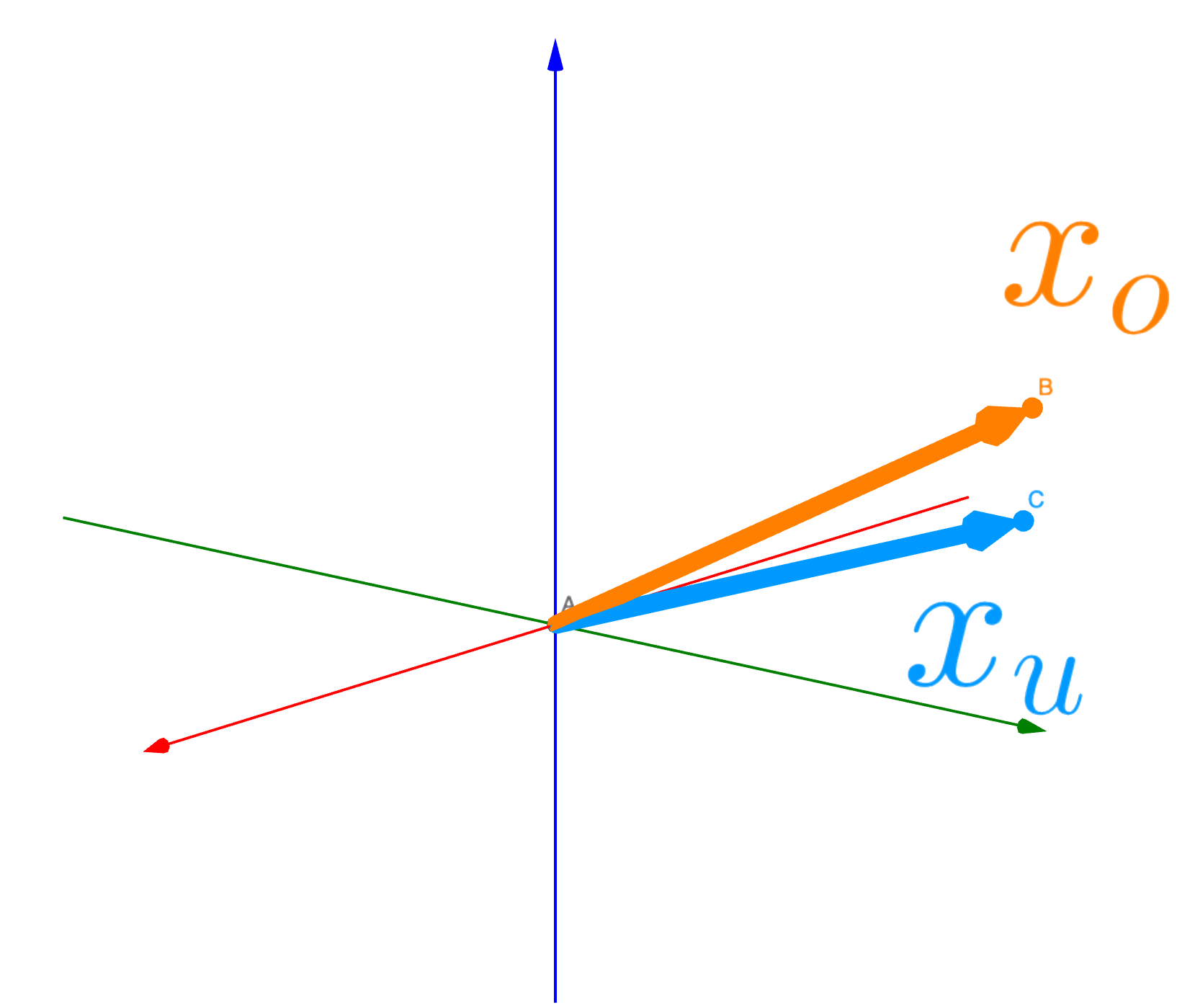
(a) Interchangeable

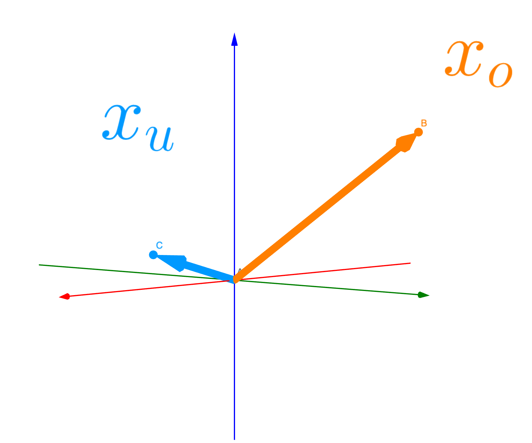
(b) Unrelated

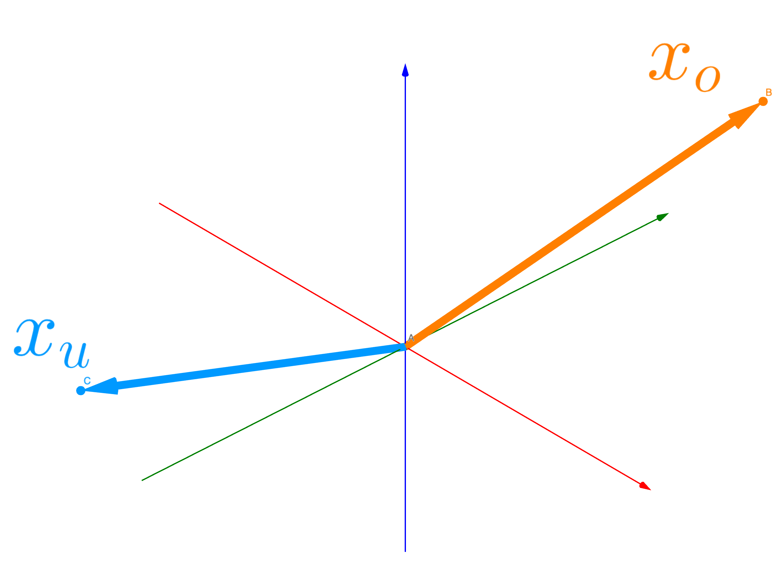
(c) Contradictory

Figure 3: Visualisation of three possible relationships between data samples. Each vector represents an update to parameters of models based on a back-propagation from a sample e.g. ${\color[rgb]{1,.5,0}{\bm{x}}_{o}}$ or ${\color[rgb]{0,0,1}{\bm{x}}_{u}}$ and their corresponding labels. Formal definitions are given below.

C.1 Interchangeable

In this case, the two gradient vectors construct a small acute angle, and projections on each other is longer than a fraction $t$ of the other vector, formally the conditions can be written as

$$\frac{\nabla_{{\bm{w}}}{\bm{z}}_{y}({\color[rgb]{0,0,1}{\bm{x}}_{u}})\cdot\nabla_{{\bm{w}}}{\bm{z}}_{y}({\color[rgb]{1,.5,0}{\bm{x}}_{o}})}{|\nabla_{{\bm{w}}}{\bm{z}}_{y}({\color[rgb]{0,0,1}{\bm{x}}_{u}})|^{2}}\geq t\wedge\frac{\nabla_{{\bm{w}}}{\bm{z}}_{y}({\color[rgb]{0,0,1}{\bm{x}}_{u}})\cdot\nabla_{{\bm{w}}}{\bm{z}}_{y}({\color[rgb]{1,.5,0}{\bm{x}}_{o}})}{|\nabla_{{\bm{w}}}{\bm{z}}_{y}({\color[rgb]{1,.5,0}{\bm{x}}_{o}})|^{2}}\geq t$$

where $t\in(\frac{1}{2},1]$. This situation is visualised in Figure 3(a).

C.2 Unrelated

In this case, the two gradient vectors are almost inter-orthogonal, formally the conditions can be written as

$$\frac{\nabla_{{\bm{w}}}{\bm{z}}_{y}({\color[rgb]{0,0,1}{\bm{x}}_{u}})\cdot\nabla_{{\bm{w}}}{\bm{z}}_{y}({\color[rgb]{1,.5,0}{\bm{x}}_{o}})}{|\nabla_{{\bm{w}}}{\bm{z}}_{y}({\color[rgb]{0,0,1}{\bm{x}}_{u}})|^{2}}\approx 0\wedge\frac{\nabla_{{\bm{w}}}{\bm{z}}_{y}({\color[rgb]{0,0,1}{\bm{x}}_{u}})\cdot\nabla_{{\bm{w}}}{\bm{z}}_{y}({\color[rgb]{1,.5,0}{\bm{x}}_{o}})}{|\nabla_{{\bm{w}}}{\bm{z}}_{y}({\color[rgb]{1,.5,0}{\bm{x}}_{o}})|^{2}}\approx 0.$$

This situation is visualised in Figure 3(b).

C.3 contradictory

In this case, the two gradient vectors are almost opposite. Like the interchangeable case, the conditions can be formally written as:

$$\frac{\nabla_{{\bm{w}}}{\bm{z}}_{y}({\color[rgb]{0,0,1}{\bm{x}}_{u}})\cdot\nabla_{{\bm{w}}}{\bm{z}}_{y}({\color[rgb]{1,.5,0}{\bm{x}}_{o}})}{|\nabla_{{\bm{w}}}{\bm{z}}_{y}({\color[rgb]{0,0,1}{\bm{x}}_{u}})|^{2}}\leq t\wedge\frac{\nabla_{{\bm{w}}}{\bm{z}}_{y}({\color[rgb]{0,0,1}{\bm{x}}_{u}})\cdot\nabla_{{\bm{w}}}{\bm{z}}_{y}({\color[rgb]{1,.5,0}{\bm{x}}_{o}})}{|\nabla_{{\bm{w}}}{\bm{z}}_{y}({\color[rgb]{1,.5,0}{\bm{x}}_{o}})|^{2}}\leq t$$

where $t\in[-1,-\frac{1}{2})$. This situation is visualised in Figure 3(c).

However, the possible causes of this case is more complicated than the above two.

• ${\color[rgb]{0,0,1}y_{u}}={\color[rgb]{1,.5,0}y_{o}}$, i.e. the two samples are from the same class. Suppose ${\color[rgb]{0,0,1}{\bm{x}}_{u}}$ is interchangeable with many other samples in the same class and ${\color[rgb]{1,.5,0}{\bm{x}}_{o}}$ is not, this may indicate that ${\color[rgb]{1,.5,0}{\bm{x}}_{o}}$ is an outlier of the class.

• ${\color[rgb]{0,0,1}y_{u}}\neq{\color[rgb]{1,.5,0}y_{o}}$, i.e. the samples are from different classes. Since the annotated data in these two classes can not be learnt by the model at the same time, our guess is that the data is not completely compatible with the learning model, or the learning model may have a wrong bias for the task.

Appendix D Further Details about Experiments in Section 3

D.1 An Extreme Example of Easy/Hard Samples Due to Interactions

In this section, we illustrate an extreme case of interchangeable sample and another extreme case of contradictory samples. To simplify the task, we assume $K=2$, i.e. a binary classification problem, and there are only two annotated samples in the training set, $({\color[rgb]{0,0,1}{\bm{x}}_{u}},{\color[rgb]{0,0,1}y_{u}})$ and $({\color[rgb]{0,0,1}{\bm{x}}_{u}},{\color[rgb]{1,.5,0}y_{o}})$. Note that the inputs are identical, and we discuss ${\color[rgb]{1,.5,0}y_{o}}={\color[rgb]{0,0,1}y_{u}}$ and ${\color[rgb]{1,.5,0}y_{o}}\neq{\color[rgb]{0,0,1}y_{u}}$ separately in the following.

1. ${\color[rgb]{1,.5,0}y_{o}}={\color[rgb]{0,0,1}y_{u}}$ In this case, the two annotated sample are actually identical, thus learning any one of them is equivalent to learning both. It is then straightforward to see that these two (identical) samples are interchangeable. Though they are identical, the one that appears later would be counted as an easy sample, since the updates on the other one automatically lead to good predictions for both.

2. ${\color[rgb]{1,.5,0}y_{o}}\neq{\color[rgb]{0,0,1}y_{u}}$ In this case, since there are only two categories, learning one of them would cancel the update due to the other one. Suppose the model is being trained in an online learning fashion, and the two samples appear in turn. Then, learning $({\color[rgb]{0,0,1}{\bm{x}}_{u}},{\color[rgb]{0,0,1}y_{u}})$ drags the model’s prediction ${\bm{q}}({\color[rgb]{0,0,1}{\bm{x}}_{u}})$ towards ${\color[rgb]{0,0,1}y_{u}}$. On the other hand, learning $({\color[rgb]{0,0,1}{\bm{x}}_{u}},{\color[rgb]{1,.5,0}y_{o}})$ drags the model’s prediction ${\bm{q}}({\color[rgb]{0,0,1}{\bm{x}}_{u}})$ towards the opposite direction ${\color[rgb]{1,.5,0}y_{o}}$. In this way, the two samples are completely contradictory to each other, and they both are difficult samples, since the learning is unlikely to converge.

D.2 Further Details about the Learning Difficulty Correlation Experiment

In this section, we illustrate more details about how we measure the learning difficulty of samples in datasets with varying sizes, as a supplement to Section LABEL:ssec:rethinking:learing_one_sample3.2. Let’s suppose that the original training set ${\mathbb{T}}$ contains $N$ samples of $K$ classes. For a given subset size $X$, we construct $\frac{N}{X}$ proper subsets of ${\mathbb{T}}$, ${\mathcal{T}}\triangleq\{{\mathbb{T}}_{1},\dots,{\mathbb{T}}_{\frac{N}{X}}\}$, of which each contains $X$ samples drawn uniformly at random from all classes without replacement. To get the Pearson correlation coefficient $\rho$ between learning difficulty of samples on ${\mathbb{T}}$ and ${\mathcal{T}}$, we run the following Algorithm 1.

1

Input:

${\mathbb{T}}=\{({\bm{x}}_{n},y_{n})\}_{n=1}^{N}$	the training set
${\bm{w}},f$	initial parameters, and the ANN to train
$E$	number of training epochs
$\eta$	learning rate

2

${\mathbb{L}}\leftarrow\{\underbrace{0,\dots,0}_{N\text{ in total}}\}$ ;

  // List of sample learning difficulty on ${\mathbb{T}}$

$\tilde{{\mathbb{L}}}\leftarrow\{\underbrace{0,\dots,0}_{N\text{ in total}}\}$ ;

  // Lists of sample learning difficulty on subsets

3

${\bm{w}}_{0}\leftarrow{\bm{w}}$ ;

  // Initialise the parameters to learn

4 for $e\leftarrow 1$ to $E$ do

5       for $n\leftarrow 1$ to $N$ do

6             ${\bm{q}}\leftarrow f({\bm{x}}_{n};{\bm{w}}_{0})$;

             $l\leftarrow-\sum_{k=1}^{K}\bm{1}(k=y_{n})\log({\bm{q}}_{k})$ ;

              // Cross-entropy loss

7             ${\mathbb{L}}_{n}\leftarrow{\mathbb{L}}_{n}+l$;

8             ${\bm{w}}_{0}\leftarrow{\bm{w}}_{0}+\eta\times\nabla_{{\bm{w}}_{0}}l$;

9            

10      

11

12for $j\leftarrow 1$ to $\frac{N}{X}$ do

       ${\bm{w}}_{j}\leftarrow{\bm{w}}$ ;

        // Initialise the parameters for subset $j$

13       for $e\leftarrow 1$ to $E$ do

14             for $n\leftarrow(j-1)\cdot X-1$ to $j\cdot X$ do // enumerate over a subset of ${\mathbb{T}}$

15                   ${\bm{q}}\leftarrow f({\bm{x}}_{n};{\bm{w}}_{j})$;

16                   $l\leftarrow-\sum_{k=1}^{K}\bm{1}(k=y_{n})\log({\bm{q}}_{k}))$;

17                   $\tilde{{\mathbb{L}}}_{n}\leftarrow\tilde{{\mathbb{L}}}_{n}+l$;

18                   ${\bm{w}}_{j}\leftarrow{\bm{w}}_{j}+\eta\times\nabla_{{\bm{w}}_{j}}l$;

19                  

20            

21      

22

Output: The Pearson correlation coefficient $\rho$ between ${\mathbb{L}}$ and $\tilde{{\mathbb{L}}}$

Algorithm 1 Correlation between Learning Difficulty on Size $N$ and Size $X$

In Section 3.2, we set $N=2000$ on MNIST. To further eliminate the effects from hyperparameters, we run Algorithm 1 on both MNIST and CIFAR-10 with varying learning rates as well as batch size. In these experiments, we train LeNet-5 on MNIST and ResNet-18 on CIFAR-10. The results and the corresponding hyperparameters are listed below:

1. this setting runs on MNIST with $N=4096,X\in\{1,4,16,64,256,1024\}$, learning rate is set to $0.1$, and batch size is $128$, the correlation results are given in Table 4 and are visualised in Figure 4;

2. this setting runs on MNIST with $N=4096,X\in\{1,4,16,64,256,1024\}$, learning rate is set to $0.001$, and batch size is $256$, the correlation results are given in Table 5 and are visualised in Figure 5;

3. this setting runs on CIFAR10 with $N=4096,X\in\{1,4,16,64,256,1024\}$, learning rate is set to $0.1$, and batch size is $128$, the correlation results are given in Table 6 and are visualised in Figure 6;

Note that the hyperparameter combinations in all the above settings are different from the experiment we ran for Figure 1. Therefore, we argue that the conclusion on learning difficulty correlations experiments consistently holds across different combinations of hyperparameters, $N$ and $X$.

Size	4096	1024	256	64	16	4	1
4096	1.0	0.8512	0.7282	0.5753	0.3865	0.2330	0.062
1024		1.0	0.8206	0.6775	0.4731	0.2888	0.0658
256			1.0	0.7856	0.5853	0.3687	0.0858
64				1.0	0.7169	0.4871	0.1566
16					1.0	0.6379	0.2303
4						1.0	0.3720
1							1.0

Table 4: The Pearson correlation coefficients $\rho$ between learning difficulty on MNIST where $N=4096,X\in\{1,4,16,64,256,1024\}$, learning rate is set to $0.1$, and batch size is $128$, i.e. setting 1. As shown in the table, larger gap between the sizes always lead to smaller $\rho$, which matches with our Prediction Prediction 1 illustrated in Section 3.2.

Size	4096	1024	256	64	16	4	1
4096	1.0	0.9096	0.7376	0.4065	0.2141	0.0695	0.0307
1024		1.0	0.8830	0.5128	0.2707	0.0858	0.0498
256			1.0	0.6782	0.3486	0.0971	0.0605
64				1.0	0.5898	0.1774	0.1598
16					1.0	0.6601	0.6023
4						1.0	0.8414
1							1.0

Table 5: The Pearson correlation coefficients $\rho$ between learning difficulty on MNIST where $N=4096,X\in\{1,4,16,64,256,1024\}$, learning rate is set to $0.001$, and batch size is $256$, i.e. setting 2. As shown in the table, larger gap between the sizes always lead to smaller $\rho$, which matches with our Prediction Prediction 1 illustrated in Section 3.2.

Size	4096	1024	256	64	16	4	1
4096	1.0	0.8433	0.5772	0.2805	0.1840	0.0628	0.0131
1024		1.0	0.7377	0.4142	0.2595	0.0950	0.0254
256			1.0	0.5409	0.3979	0.1352	0.0345
64				1.0	0.4082	0.1493	0.0427
16					1.0	0.1844	0.0673
4						1.0	0.0912
1							1.0

Table 6: The Pearson correlation coefficients $\rho$ between learning difficulty on CIFAR10 where $N=4096,X\in\{1,4,16,64,256,1024\}$, learning rate is set to $0.1$, and batch size is $128$, i.e. setting 3. As shown in the table, larger gap between the sizes always lead to smaller $\rho$, which matches with our Prediction Prediction 1 illustrated in Section 3.2.

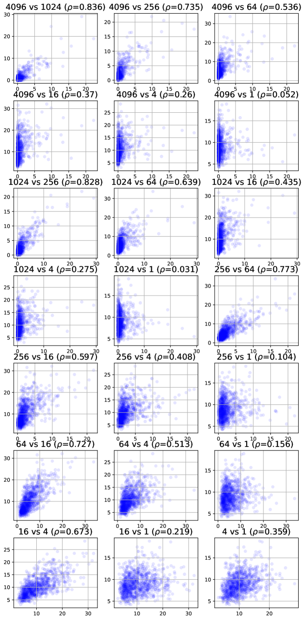
Figure 4: Visualisation of the correlation between learning difficulty on MNIST where $N=4096,X\in\{1,4,16,64,256,1024\}$, learning rate is set to $0.1$, and batch size is $128$, i.e. setting 1. Note that we plot only the correlation between $1000$ samples in order to keep the plots readable.

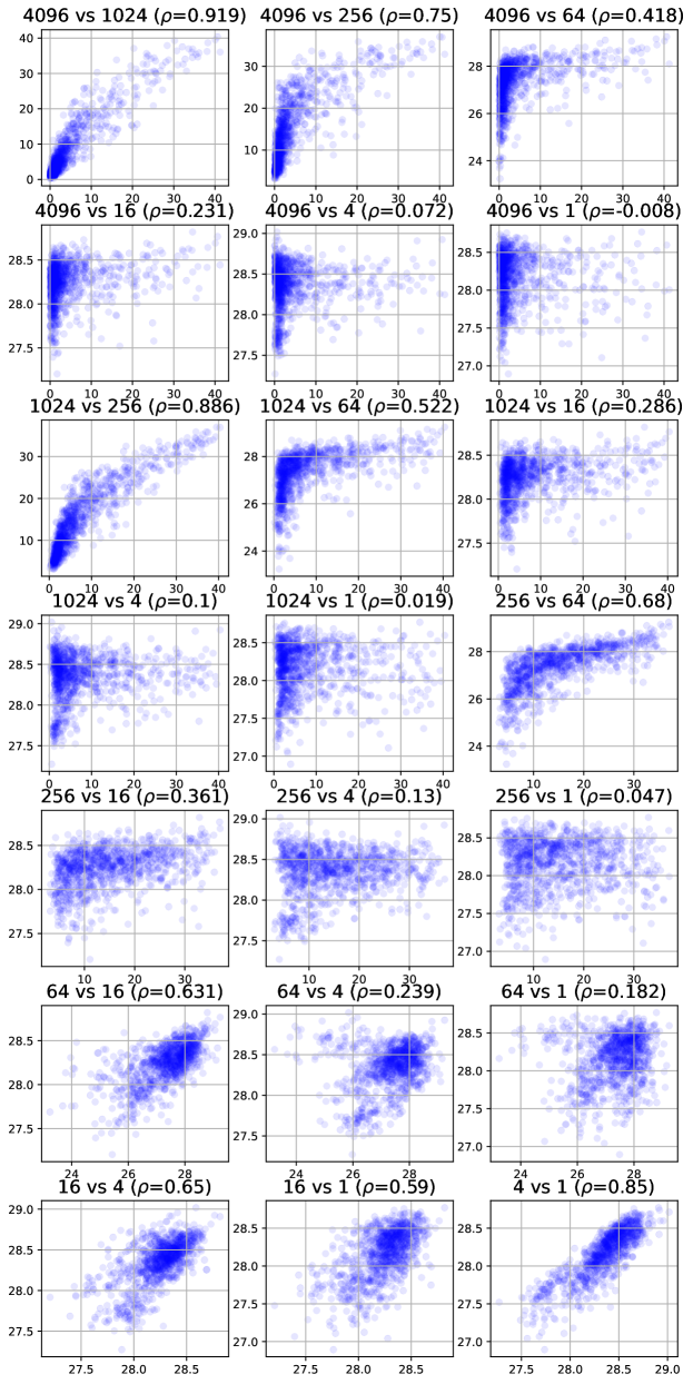
Figure 5: Visualisation of the correlation between learning difficulty on MNIST where $N=4096,X\in\{1,4,16,64,256,1024\}$, learning rate is set to $0.001$, and batch size is $256$, i.e. setting 2. Note that we plot only the correlation between $1000$ samples in order to keep the plots readable.

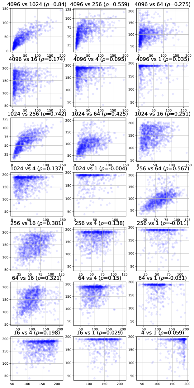
Figure 6: Visualisation of the correlation between learning difficulty on CIFAR10 where $N=4096,X\in\{1,4,16,64,256,1024\}$, learning rate is set to $0.1$, and batch size is $128$, i.e. setting 3. Note that we plot only the correlation between $1000$ samples in order to keep the plots readable.

D.3 Further Details about the Learning Difficulty Control Experiment

In this section, we provide more details about the learning difficulty control experiment illustrated in Section 3.2. We first show the centroids of largest cluster obtained through farthest point clustering, of which more details can be found in Appendix D.5, of each class in MNIST and CIFAR10 in Figure 7 and Figure 8 respectively.

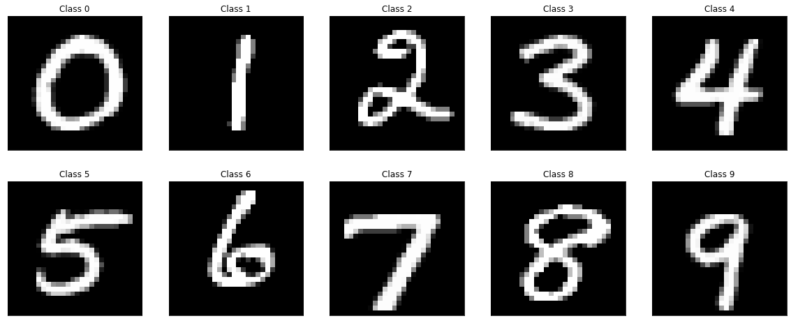
Figure 7: Target samples of each class in MNIST found by FPC with lpNTK as the similarity metric.

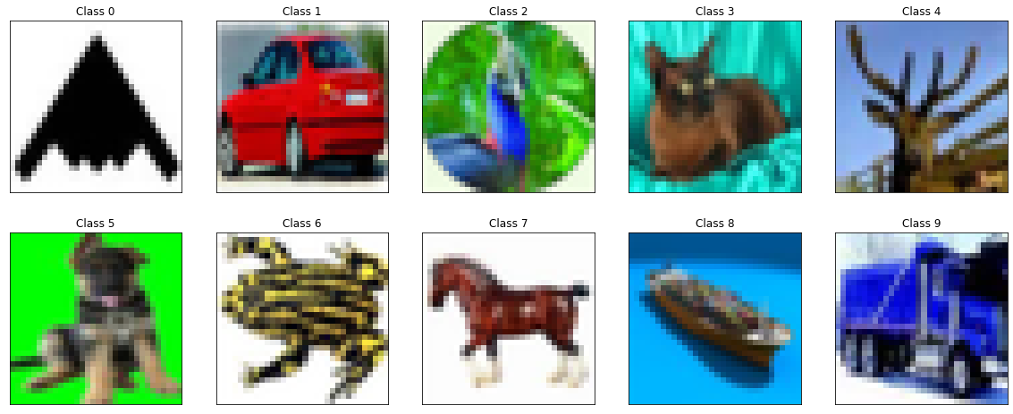
Figure 8: Target samples of each class in CIFAR10 found by FPC with lpNTK as the similarity metric.

Then, we show the samples that are the most interchangeable to the targets, thus make the targets easier to learn, on MNIST and CIFAR10 in Figure 9 and Figure 10 respectively. It is worth noting that the most interchangeable samples to the targets found by lpNTK are not necessarily the most similar samples to the targets in the input space. Take the “car” class in CIFAR10 (the second row of Figure 10) for example, the target is a photo of a red car from the left back view, and the third most interchangeable sample to it is a photo of a yellow from the front right view. At the same time, the fourth and fifth most interchangeable samples are both photos of red cars, thus they have shorter distance to the targets in the input space due to the large red regions in them. However, under the lpNTK measure, the fourth and fifth red cars are less interchangeable/similar to the target red car than the third yellow car. This example shows that our lpNTK is significantly different from the similarity measures in the input space.

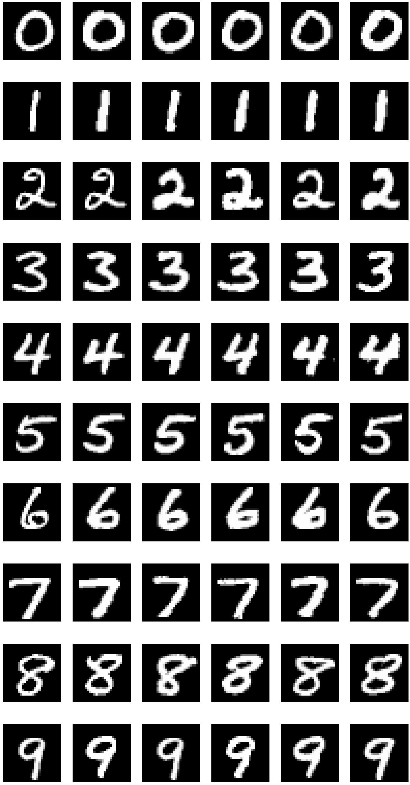
Figure 9: Samples that are the most interchangeable to the targets in MNIST. The leftmost column is the target samples that are also shown in Figure 7. The remaining 5 columns are the most interchangeable samples to the targets in each class.

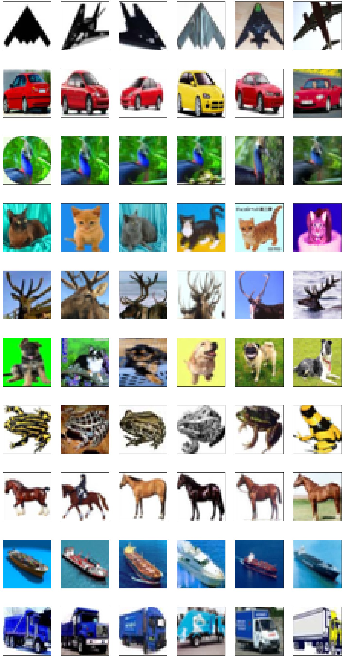
Figure 10: Sample that are the most interchangeable to the targets in CIFAR10. The leftmost column is the target samples that are also shown in Figure 8. The remaining 5 columns are the most interchangeable samples to the targets in each class.

We also show the samples that are medium interchangeable to the targets, thus make the targets medium easy to learn, on MNIST and CIFAR10 in Figure 11 and Figure 12 respectively.

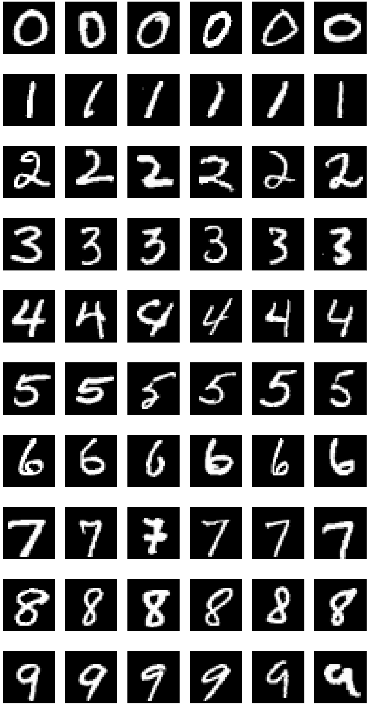
Figure 11: Samples that are the medium interchangeable to the targets in MNIST. The leftmost column is the target samples that are also shown in Figure 7. The remaining 5 columns are the medium interchangeable samples to the targets in each class.

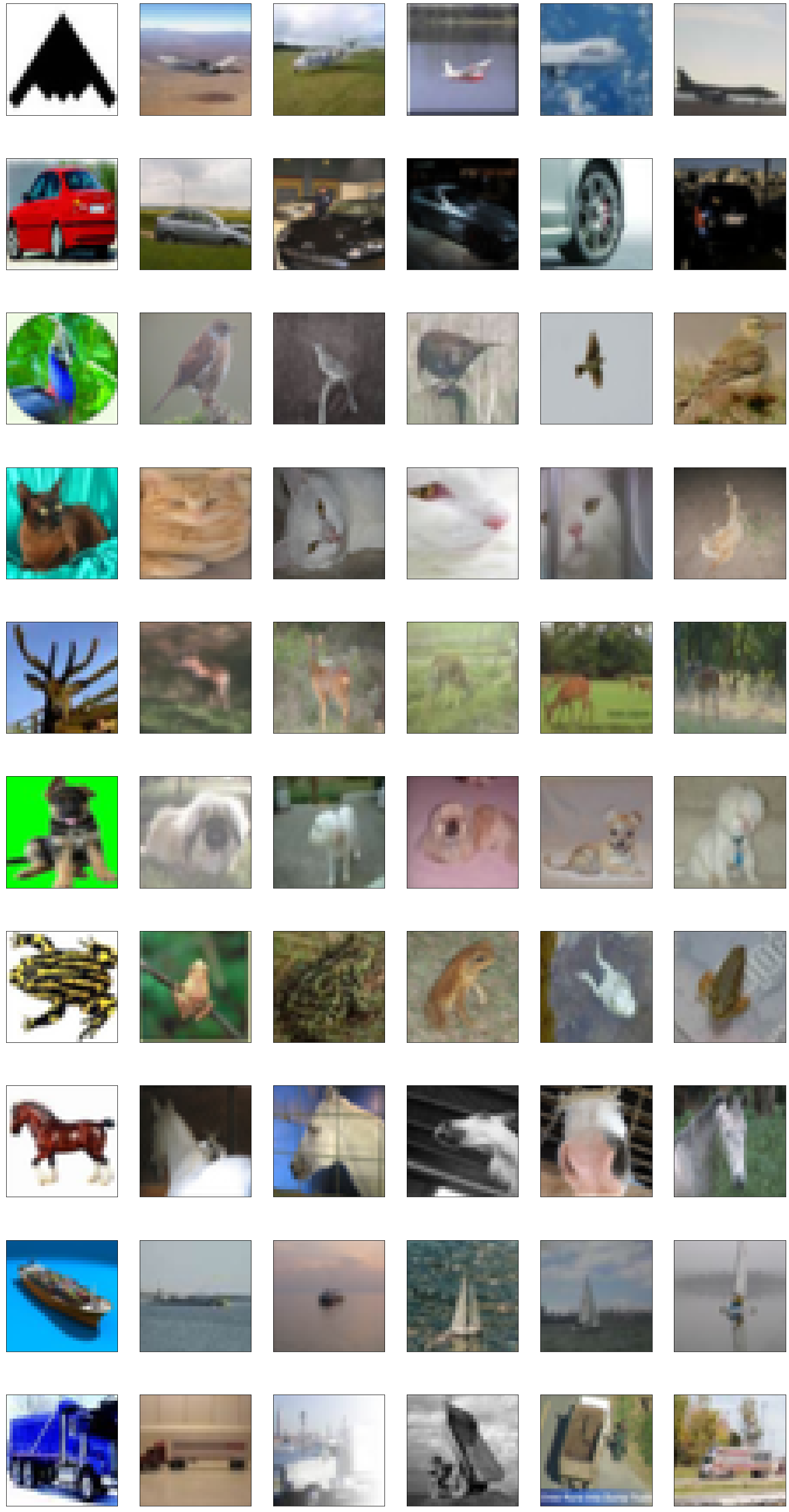
Figure 12: Sample that are the medium interchangeable to the targets in CIFAR10. The leftmost column is the target samples that are also shown in Figure 8. The remaining 5 columns are the medium interchangeable samples to the targets in each class.

Finally, we show the samples that are the most non-interchangeable to the targets, thus make the targets hard to learn, on MNIST and CIFAR10 in Figure 13 and Figure 14 respectively. We observed that these samples from the tail clusters are more likely to share features appearing in other classes. An example is the class “6” shown in the seventh row of Figure 13. As can be seen there, the second to fourth most non-interchangeable to the target look more like “4” than the others. Inspired by this observation, we argue that samples in the tail classes should be annotated with multiple labels rather than a single label, since they may contain similar “feature” from other classes. However, limited to the scope by this work, we leave this question to the future works.

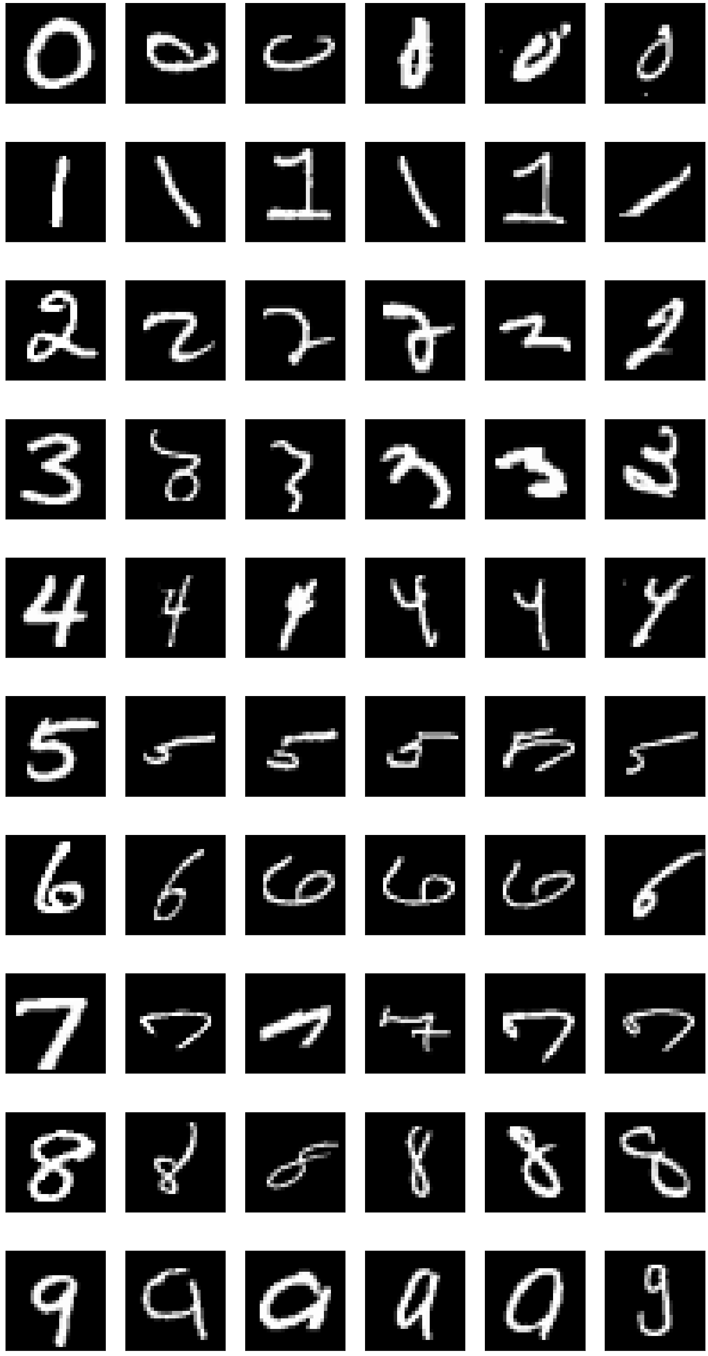
Figure 13: Samples that are the most non-interchangeable to the targets in MNIST. The leftmost column is the target samples that are also shown in Figure 7. The remaining 5 columns are the most non-interchangeable samples to the targets in each class.

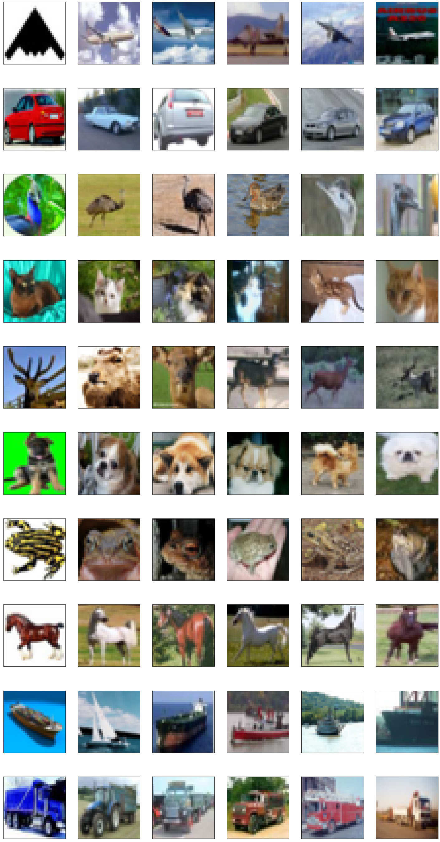
Figure 14: Sample that are the most non-interchangeable to the targets in CIFAR10. The leftmost column is the target samples that are also shown in Figure 8. The remaining 5 columns are the most non-interchangeable samples to the targets in each class.

D.4 Further Details about the Forgetting Event Prediction Experiment

In this section, we illustrate more details about how we predict the forgetting events with our eNTKlpNTK, as a supplement to Section 3.3. Let’s suppose at training iteration $t$, the parameter of our model ${\bm{w}}^{t}$ is updated with a batch of samples ${\mathbb{B}}^{t}=\{({\bm{x}}^{t}_{i},y^{t}_{i})\}_{i=1}^{B}$ of size $B$, thus becomes ${\bm{w}}^{t+1}$. Then, at the next iteration $t+1$, we update the model parameters ${\bm{w}}^{t+1}$ with another batch of samples ${\mathbb{B}}^{t+1}=\{({\bm{x}}^{t+1}_{i},y^{t+1})_{i}\}_{i=1}^{B}$ to ${\bm{w}}^{t+2}$. We then run found that the predictions on a large number of samples at the beginning of training are almost uniform distributions over classes, thus the prediction error term in Equation 2 is likely to be $[-\frac{1}{K},\dots,1-\frac{1}{K},\dots,-\frac{1}{K}]^{\mathsf{T}}$. To give a more accurate approximation to the change of predictions at the beginning of training, we therefore replace the ${\bm{s}}(y)$ in Equation 3 with $\tilde{{\bm{s}}}(y)=[-1,\dots,\underbrace{K-1}_{y-\mbox{th entry}},\dots,-1]^{\mathsf{T}}$ and denote this variant of our lpNTK as $\tilde{\kappa}$. We then propose the following Algorithm 2 to get the confusion matrix of the performance of predicting forgetting events with eNTK$\tilde{\kappa}$.

1

Input:

${\mathbb{B}}^{t}=\{({\bm{x}}^{t}_{i},y^{t}_{i})\}_{i=1}^{B}$	the batch of samples at $t$
${\mathbb{B}}^{t+1}=\{({\bm{x}}^{t+1}_{i},y^{t+1})_{i}\}_{i=1}^{B}$	the batch of samples at $t+1$
${\bm{w}}^{t},{\bm{w}}^{t+1},{\bm{w}}^{t+2}$	the saves parameters at time-step $t$, $t+1$, and $t+2$
$\eta$	learning rate

2

${\mathbb{F}}\leftarrow\{\underbrace{0,\dots,0}_{B\text{ in total}}\}$ ;

  // List to record whether forgetting events happen

$\hat{{\mathbb{F}}}\leftarrow\{\underbrace{0,\dots,0}_{B\text{ in total}}\}$ ;

  // List to record the predicted forgetting events

3

4for $i\leftarrow 1$ to $B$ do

5       if $\arg\max{\bm{q}}^{t+1}({\bm{x}}_{i}^{t};{\bm{w}}^{t+1})=y_{i}^{t}\wedge\arg\max{\bm{q}}^{t+2}({\bm{x}}_{i}^{t};{\bm{w}}^{t+2})\neq y_{i}^{t}$ then

             ${\mathbb{F}}_{i}\leftarrow 1$ ;

              // Forgetting event happens

6            

7      $\Delta q_{i}\leftarrow 0$;

8       for $j\leftarrow 1$ to $B$ do

9             $\Delta q_{i}\leftarrow\Delta q_{i}+\tilde{\kappa}({\bm{x}}^{t}_{i},{\bm{x}}^{t+1}_{j};{\bm{w}}^{t+1})$;

10            

11      $\Delta{\bm{q}}_{i}\leftarrow\Delta q_{i}\cdot\begin{bmatrix}-1\\ \dots\\ K-1\\ \dots\\ -1\end{bmatrix}$ where $K-1$ is the $y_{i}^{t}$-th element;

12       if $\arg\max{\bm{q}}^{t+1}({\bm{x}}_{i}^{t};{\bm{w}}^{t+1})=y_{i}^{t}\wedge\arg\max\left[{\bm{q}}^{t+1}({\bm{x}}_{i}^{t};{\bm{w}}^{t+1})+\Delta{\bm{q}}_{i}\right]\neq y_{i}^{t}$ then

             $\hat{{\mathbb{F}}}_{i}\leftarrow 1$ ;

              // Predicted forgetting events

13            

14      

15

Output: The precision, recall, and F1-score of $\hat{{\mathbb{F}}}$ with ${\mathbb{F}}$ as ground truth

Algorithm 2 Predict forgetting events with eNTKa variant of lpNTK $\tilde{\kappa}$

D.5 Farthest Point Clustering with lpNTK

In this section, we illustrate more details about how we cluster the training samples based on farthest point clustering (FPC) and lpNTK. Suppose that there are $N$ samples in the training set, $\{({\bm{x}}_{i},y_{i})\}^{N}_{i=1}$, and the lpNTK between a pair of samples is denoted as $\kappa(({\bm{x}},y),({\bm{x}}^{\prime},y^{\prime}))$. The FPC algorithm proposed by gonzalez1985clustering running with our lpNTK is demonstrated in the following Algorithm 3.

Input: Dataset $\{({\bm{x}}_{i},y_{i})\}^{N}_{i=1}$, The number of centroids $M$

Output: Cluter centroids $\{c_{1},\dots,c_{M}\}$, LIst of samples indices in all clusters: $\{{\mathbb{L}}_{1},\dots,{\mathbb{L}}_{M}\}$

$N_{c}\leftarrow 1$ ;

  // Number of established clusters

$c_{1}\leftarrow\arg\max_{i}\kappa(({\bm{x}}_{i},y_{i}),({\bm{x}}_{i},y_{i}))$ ;

  // Centroid of the first cluster

${\mathbb{L}}_{1}\leftarrow\{i\neq c_{1}\}^{N}_{i=1}$ ;

  // List of sample indices in the first clsuter

1 while $N_{c}<M$ do

       $d\leftarrow\infty,c_{new}\leftarrow-1$ ;

        // 1. Find the controid for the new cluster

2       for $j\leftarrow 1$ to $N_{c}$ do

3             if $\min_{j^{\prime}\in{\mathbb{L}}_{j}}\kappa(({\bm{x}}_{c_{j}},y_{c_{J}}),({\bm{x}}_{j^{\prime}},y_{j^{\prime}}))<d$ then

4                   $d\leftarrow\min_{j^{\prime}\in{\mathbb{L}}_{j}}\kappa(({\bm{x}}_{c_{j}},y_{c_{J}}),({\bm{x}}_{j^{\prime}},y_{j^{\prime}}))$;

5                   $c_{new}\leftarrow\arg\min_{j^{\prime}\in{\mathbb{L}}_{j}}\kappa(({\bm{x}}_{c_{j}},y_{c_{J}}),({\bm{x}}_{j^{\prime}},y_{j^{\prime}}))$;

6                  

7            

      $N_{c}\leftarrow N_{c}+1,c_{N_{c}}\leftarrow c_{new},L_{N_{c}}\leftarrow\varnothing$ // 2. Move samples that are closer to the new centroid to the new cluster

8       for $j\leftarrow 1$ to $N_{c}-1$ do

9             for $i\in{\mathbb{L}}_{j}$ do

10                   if $\kappa(({\bm{x}}_{i},y_{i}),({\bm{x}}_{c_{j}},y_{c_{j}}))<\kappa(({\bm{x}}_{i},y_{i}),({\bm{x}}_{c_{N_{c}}},y_{c_{N_{c}}}))$ then

11                         ${\mathbb{L}}_{j}\leftarrow{\mathbb{L}}_{j}\setminus\{i\}$;

12                         ${\mathbb{L}}_{N_{c}}\leftarrow{\mathbb{L}}_{N_{c}}\cup\{i\}$;

13                        

14                  

15            

16      

Algorithm 3 Farthest Point Clustering with lpNTK

To show that the distribution of clusters sizes are heavily long-tailed on both MNIST and CIFAR-10, i.e. there are a few large clusters and many small clusters, we use $M=10\%\times N$ here. We sort the clusters from FPC first by size, then show the sizes of the top-$30$ on MNIST and CIFAR10 in Figure 15. It is straightforward to see that most of the samples are actually in the head cluster, i.e. the largest cluster. There are a further $5-20$ clusters containing more than one sample, then the remaining clusters all contain just a single sample. This indicates that the cluster distribution is indeed long-tailed.

(a) MNIST

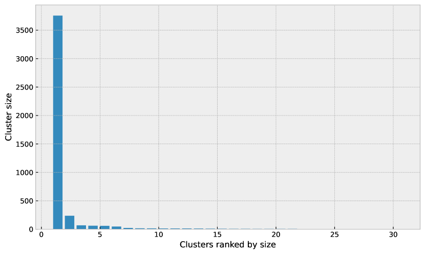
(b) CIFAR-10

Figure 15: Number of samples in the top-$30$ clusters ranked by sizes on MNIST and CIFAR-10. The number of clusters equals to $10\%$ of the original training set’s size, and both used categories indexed $0$ as an example.

Appendix E Redundant Samples and Poisoning Samples

E.1 Redundant Samples

Suppose there are two samples ${\bm{x}}_{1}$ and ${\bm{x}}_{2}$ from the same class, and their corresponding gradient vectors in the lpNTK feature space are drawn as two solid arrows in Figure 16. The ${\bm{x}}_{1}$ can be further decomposed into two vectors, ${\bm{x}}_{1}^{\prime}$ which has the same direction as ${\bm{x}}_{2}$ and ${\bm{x}}_{1}^{\prime\prime}$ whose direction is perpendicular to ${\bm{x}}_{2}$, and both are drawn as dashed arrows in Figure 16. Since ${\bm{x}}_{1}^{\prime}$ is larger than ${\bm{x}}_{2}$, this means that a component of ${\bm{x}}_{1}$ is larger than ${\bm{x}}_{2}$ on the direction of ${\bm{x}}_{2}$. Further, this shows that learning ${\bm{x}}_{1}$ is equivalent to learning ${\bm{x}}_{2}$ (times some constant) and a hypothetical samples that is orthogonal to ${\bm{x}}_{2}$. In this case, the sample ${\bm{x}}_{2}$ is said to be redundant.

Figure 16: A hypothetical redundant sample (${\bm{x}}_{2}$) example.

E.2 Poisoning Samples

Data poisoning refers to a class of training-time adversarial attacks wang2022lethal: the adversary is given the ability to insert and remove a bounded number of training samples to manipulate the behaviour (e.g. predictions for some target samples) of models trained using the resulted, poisoned data. Therefore, we use the name of “poisoning samples” here rather than “outliers” or “anomalies” to emphasise that those samples lead to worse generalisation.

More formally, for a given set of samples ${\mathbb{T}}$, if the averaged test accuracy of the models trained on ${\mathbb{X}}\subset{\mathbb{T}}$ is statistically significantly greater than the models trained on ${\mathbb{T}}$, the samples in ${\mathbb{T}}\setminus{\mathbb{X}}$ are defined as poisoning samples.

To better illustrate our findings about poisoning samples, we first illustrate a hypothetical FPC results, as shown in Figure 17. There are 5 resulted clusters, and the number of samples in each cluster is $7,2,1,1,1$. Back to the three types of relationships defined in Section 3, samples in the same cluster (e.g. the blue dots) would be more likely to be interchangeable with each other, and samples from different clusters (e.g. the yellow, green, and red dots) would be more likely to be unrelated or contradictory.

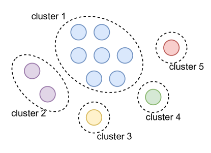
Figure 17: An example of farthest point clustering result.

Although those samples in the tail did not seem to contribute much to the major group, the interesting thing is that they are not always poisoning. That is, the poisoning data are inconsistent over the varying sizes of the pruned dataset.

Let’s denote the original training set as ${\mathbb{T}}$, and the pruned dataset as ${\mathbb{X}}$. When a large fraction of data can be kept in the pruned dataset, e.g. $|{\mathbb{X}}|/|{\mathbb{T}}|>85\%$, removing some samples that are more interchangeable with the others, or equivalently from the head cluster, would benefit the test accuracy, as demonstrated in Section 4.3. That is, in such case, the poisoning samples are the samples in the largest cluster, e.g. the blue dots in Figure 17.

However, where only a small fraction of data can be kept, e.g. $5\%$ or $1\%$, we find that the poisoning samples are the samples from the tail clusters, e.g. the yellow/green/red dot in Figure 17. This finding matches with the conclusions from sorscher2022beyond. To verify it, we first randomly sample $5\%$ from the MNIST training set, and put them all together in a training set ${\mathbb{T}}_{1}$. In the meantime, we sample the same amount of data only from the largest cluster obtained on MNISTin Section LABEL:ssec:rethinking:fpc, and put them all together in another training set ${\mathbb{T}}_{2}$. We then compare the generalisation performance of LeNet models trained with ${\mathbb{T}}_{1}$ and ${\mathbb{T}}_{2}$, and we try two fractions, $1\%$ and $5\%$. The results are shown in the following Figure 18.

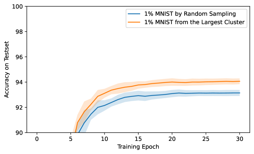
(a) 1%

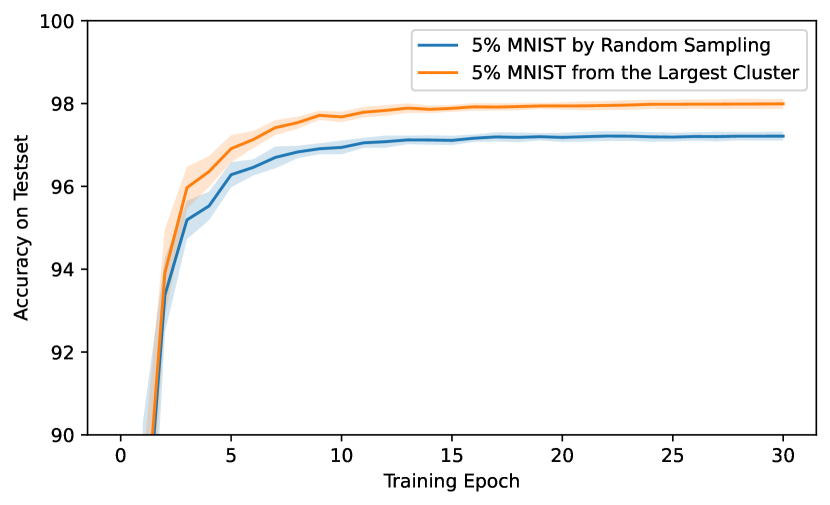
(b) 5%

Figure 18: Test accuracy over training epochs of models trained with $X\%$ data sampled with different strategies. The lines are averaged across $10$ different runs, and the shadow areas show the corresponding standard deviation. The plots show that sampling from the largest FPC cluster can lead to higher generalisation performance when only a small fraction of data can be kept in the pruned training sets.

As shown in Figure 18, in both $1\%$ and $5\%$ cases, keeping only the samples from the largest cluster obtained via FPC with lpNTK lead to higher test accuracy than sampling from the whole MNIST training set. This verifies our argument that the most interchangeable samples are more important for generalisation when only a few training samples can be used for learning.

Lastly, we want to give a language learning example to further illustrate the abover above argument. Let’s consider the plural nouns. We just need to add -s to the end to make regular nouns plural, and we have a few other rules for the regular nouns ending with e.g. -s, -sh, or -ch. Whereas, there is no specific rule for irregular nouns like child or mouse. So, the irregular nouns are more likely to be considered as samples in the tail clusters, as they are more dissimilar to each other. For an English learning beginner, the most important samples might be the regular nouns, as they can cover most cases of changing nouns to plurals. However, as one continues to learn, it becomes necessary to remember those irregular patterns in order to advance further. Therefore, suppose the irregular patterns are defined as in the tail clusters, they may not always be poisoning for generalisation performance.