![[Uncaptioned image]](/html/2401.08786/assets/x1.png)
Supersymmetric Virasoro Minimal Strings
Abstract
A random matrix model definition of a family of supersymmetric extensions of the Virasoro minimal string of Collier, Eberhardt, Mühlmann, and Rodriguez is presented. An analysis of the defining string equations shows that the models all naturally have unambiguous non-perturbative completions, which are explicitly supplied by the double-scaled orthogonal polynomial techniques employed. Perturbatively, the multi-loop correlation functions of the model define a special supersymmetric class of “quantum volumes”, generalizing the prototype case. For two of the models the volumes vanish to all orders in the perturbative topological expansion. This amounts to a prediction for expected related computations in 3D gravity, intersection theory, and 2D dilaton gravity.
Introduction—The Virasoro minimal string (VMS) recently presented in ref. Collier et al. (2023) is an exciting new kind of critical string theory. It was shown to be perturbatively (in world-sheet topology) equivalent to a double-scaled 111The double-scaling limitBrezin and Kazakov (1990); *Douglas:1990ve; *Gross:1990vs; *Gross:1990aw takes a large limit of an matrix model while tuning parameters in its potential to a critical point, yielding a model of 2D gravity. random matrix model whose leading density of states is the universal Cardy density for states of energy in a 2D conformal field theory (CFT). (Here, parameterizes the central charge of a component of the construction: .) The world-sheet model of the VMS can either be thought of as a model of two coupled 2D Liouville theories, or (after a field redefinition) a model of 2D gravity with a Jackiw-Teiteboim-like Jackiw (1985); *Teitelboim:1983ux dilaton coupling, but with a more general potential, useful in the study of the near-horizon dynamics of black holes. Correlation functions of the VMS theory were also shown to be captured by an intersection theory computation of the partition function of a 3D gravity on a certain surface. These connections unite several techniques and ideas from different areas of low dimensional quantum gravity research, so it is likely that this type of string theory construction will potentially lead to new illuminating results in the program of quantum gravity.
A very natural next step (anticipated in ref. Collier et al. (2023), but not explored), is to define a supersymmetric Virasoro minimal string, starting with the supersymmetric “Cardy” density of states formula, (Eq. (1) below). This Letter will do just that, using a fully non-perturbative random matrix model approach, capturing the world–sheet topological expansion and much more besides. The output will be a family of such string theories for each . An immediate observation will be that all the models turn out to be unambiguously non-perturbatively well-defined (this is only true for the case in the ordinary VMS). Moreover, various special features of the construction will have immediate predictions for the 3D gravity and 2D dilaton gravity models to which this is expected to connect.
The Approach—Following ref. Collier et al. (2023)’s presentation of the VMS, ref. Johnson (2024) showed how to formulate its random matrix description fully non-perturbatively by casting it into orthogonal polynomial language. There were two key steps:
(1) Get input from the leading density of states, determining the required double-scaled potential of the matrix model by writing it as a sum of the appropriate basic multi-critical matrix models, which amounts to writing
for
specific numbers . The function is the leading piece of , the double-scaled orthogonal polynomial recursion coefficient, while is the surviving part of what was (before double scaling) the discrete orthogonal polynomial index. (Ref. Castro (2024) also independently completed step (1) for ordinary VMS.)
(2) Determine and solve the relevant non-linear ordinary differential equation (the “string equation”) for . The orthogonal polynomials themselves are then recovered as wavefunctions of an associated Schrödinger problem, with as the potential.
This Letter will show how do the above steps to define an supersymmetric VMS, showing that the resulting equations defining the random matrix model give a compelling definition of a family of string theories. Already at step (1) the leading order string equation that results turns out to have striking properties that protect it (for all ) from pathologies that could have spoiled finding a non-perturbative completion. At step (2) the non-perturbative string equation describing the complete theory then readily supplies perturbative topological expansions for the physics, as well as solutions supplying the full non-perturbative physics of both orientable and non-orientable theories.
Recasting as Multi-critical Models—Beginning with the universal Cardy expression for the density of (NS-R) states with weight in an CFT and writing defines: 222Scott Collier and Henry Maxfield have an unpublished derivation of this formula, obtained from exploring crossing properties of Virasoro characters, along the lines of ref. Maxfield (2019).
| (1) |
with and , . The factor (or 0) in the Ramond (or Neveu-Schwarz) sector. Below, will be engineered as the leading density of states of a world-sheet gravity model. Meanwhile, the critical string construction analogous to that of the ordinary Virasoro minimal string has Collier et al. (2023) a spacelike (super)-Liouville with , , and as defined above, and also a (timelike) (super)-Liouville with , and , such that and .
In Eq. (1), is the topological expansion parameter, and is an extremal entropy in the 2D gravity picture. 2D Euclidean world-sheets with Euler characteristic (where counts handles and counts boundaries) come with a factor . Below, is identified with the (renormalized) expansion parameter of the double-scaled matrix model. The density above is the leading order (disc) density.
Notice that the low energy tail of is , characteristic of a “hard edge” matrix model. This is consistent with the fact that the lowest energy of a supersymmetric system is , and so in the random matrix description there should be a hard wall there that stops energy eigenvalues from flowing to . Notice also that when , becomes (after a rescaling of ) the leading spectral density of JT supergravity, for which this property has already been incorporated into a random matrix model description, perturbatively Stanford and Witten (2020) and non-perturbatively Johnson (2021a, b); Johnson et al. (2021). The hard edge model used was a random matrix model of type in the Altland-Zirnbauer (AZ) Altland and Zirnbauer (1997) classification. This certainly should not change by varying , so this will the kind of model sought here, and cases with and or 2 will be the focus.
If is indeed a double-scaled random matrix model’s leading spectral density, it is to be expected that:
| (2) |
where the previously mentioned function satisfies , and the and are determined by this matching. By expanding both sides in , or by directly inverting the integral transform Johnson and Rosso (2021), some algebra yields the pleasing result:
| (3) |
and so the leading string equation can be written as:
| (4) |
Here is the modified Bessel function in of order . Comparison with the results derived in ref. Johnson (2024) (and independently in ref. Castro (2024)) for the ordinary VMS will reveal a close similarly. In fact the only adjustment is that while there was a difference between pieces involving and those involving , now there is a sum!
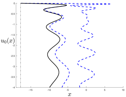
The next step is to check whether there is any problematic multi-valuedness of that would imply Johnson and Rosso (2021); Johnson (2021c) semi-classical obstructions to finding an unambiguous non-perturbative definition, as was done in the ordinary VMS case Collier et al. (2023); Johnson (2024); Castro (2024). There, the only case that survived was , where the multi-valuedness present was all at , outside the integration region used to define the density (and other matrix model quantities). Undulations from both and sectors (arising when ) inevitably spilled into . Here, it all looks generically to be problematic again, since those sectors both contribute again for general . However something rather excellent happens: vanishes at instead of zero, and for all the undulations do not stretch to smaller than this. To establish this, note that in this region, the case is the curve , which vanishes at , and never returns to this value of because of the decaying nature of Bessel undulations. For other , the undulations are pushed further to the right by a purely additive contribution. Since the integral in the region should stop where , which is , all cases have a harmless multi-valuedness. The relevant parts of with three cases of is shown in figure 1.
Meanwhile, for the regime, a different solution is used, as is familiar from analogous cases studied in the JT gravity context. It is simply from all the way to . That this is correct is consistent with the fact that the key leading term in the spectral density is generated by the right hand side of relation (2) as . It is surprising that there is a jump in the -integration (from to 0) in order for everything to work so nicely. This mirrors a surprising such jump discovered recently in the context of JT supergravity. Johnson (2023)333The lesson seems to be that for supersymmetric cases (where part of the defining -integral always runs to ), previous examples where the integral in the regime ends at were simply special cases. Moreover the case with non-zero threshold energy showed that the integral in the sector needn’t start at !
Step (1) has now been completed, and it has been shown that the leading string equation that results for for all nimbly avoids showing any semi-classical avatars of non-perturbative problems. Is time to see how this all fits into a full random matrix model definition.
The Full Non-Perturbative Definition—Recall that the topological expansion parameter is , and for the closed string sector where the ellipses denote non-perturbative parts. Actually, is the second derivative of the partition function of the string theory, nicely expressed through:
| (5) |
defining the topological expansion for the world-sheets.
The appropriate non-linear ordinary differential equation for defining the full function in this case is:
| (6) |
with where the are polynomials (see below) in and its -derivatives. This ODE arose in early studies Dalley et al. (1992a); *Dalley:1992br; *Dalley:1991vr; *Morris:1991cq; *Dalley:1991xx; *Anderson:1991ku of ensembles of positive matrices (later identified to be of type in the AZ classification). The are the “Gel’fand-Dikii” Gel’fand and Dikii (1975) differential polynomials in and its derivatives, normalized here so that the non-derivative part has unit coefficient: where means the th -derivative. e.g., , , , etc.
The solutions needed here are specified by boundary conditions that can be written for , where the string equation becomes , with :
| (7) |
The discussion above has precisely determined the , and so the definition (and hence step (2)) is complete. Different values of the parameter correspond to distinct random matrix ensembles. Both integer and half-integer are allowed, and and will be the focus. It is natural to declare that they each define a distinct kind of supersymmetric Virasoro minimal string. This is consistent with the limit where these become a known Stanford and Witten (2020) family of JT supergravity models. Just as in that limit, the simple half-integer cases are very special, as will be discussed. Notably, they are unorientable theories, while is orientable.
Non-Perturbative Results—The next step is to solve equation (6) for with the boundary conditions (7). The string equation is formally of infinite order, since each controls a term with derivatives and all the are turned on (). However ref. Johnson (2021b) noted that since the decrease swiftly enough in size as increases, a sensible truncation of the equation can be done that can capture the physics up to any desired accuracy.
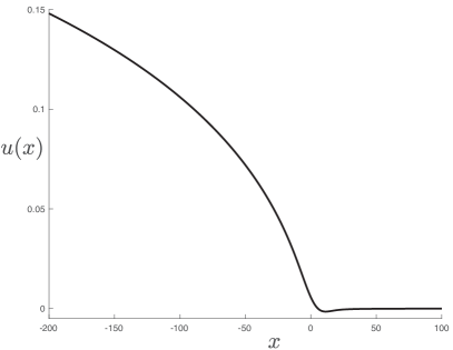
Those methods were used here to generate solutions for various examples. Figure 2 shows the case for , .
Recall that is the scaling limit of the recursion coefficient from which all the orthogonal polynomials can be determined, and labels the index on the orthogonal polynomials, now itself a continuous coordinate in the large scaling limit. The orthogonal polynomials themselves become functions in the limit, where is the scaling piece of the (continuous) eigenvalue coordinate near the end of the leading distribution. Once is known, it turns out that the are determined (up to normalization) as wavefunctions of a Schrödinger problem for which is the potential:
| (8) |
Many things can be computed in the random matrix model with the . A fundamental object is:
| (9) |
a kernel whose derivation and uses are reviewed in this context in ref. Johnson (2022). Knowing it fully non-perturbatively (via the ) allows for physics that is entirely inaccessible in topological perturbation theory to be probed. The diagonal of is the spectral density:
| (10) |
Its leading piece, met earlier in equation (1) comes from using the leading WKB form of in the limit.
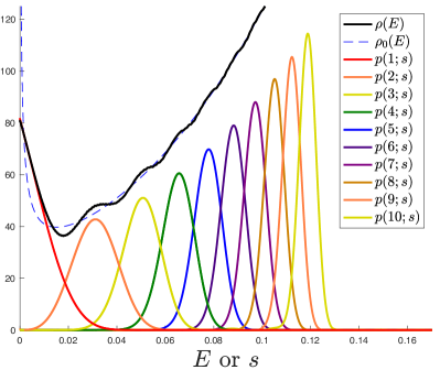
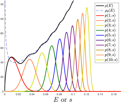
As an example of these computations, is shown as top the dark solid lines in figures 3 and 4 (for the cases of , and , with ). The dashed line is the leading spectral density (1) for . Also shown is an especially intrinsically non-perturbative structure computable with (as kernel in a Fredholm problem): The set of curves giving the probability that the th eigenvalue of a matrix in the ensemble takes the value . This is information about the underlying discrete microscopic physics of the 2D quantum gravityJohnson (2021d), recasting the continuous spectral density as a discrete sum of peaks:
An important observable is the Euclidean 2D gravity partition function, the Laplace transform of the spectral density: , where is the matrix. It is a particular kind of loop operator with length . In fact, for the Virasoro minimal string, on a surface of genus the –point correlation function is built (generalizing the construction in ref. Saad et al. (2019) involving trumpet factors) from quantities , (where are Liouville momenta setting the length of geodesic boundaries).
These are referred to in ref. Collier et al. (2023) as “quantum volumes”, generalizing the Weil-Petersson volumes on the moduli space of bordered hyperbolic Riemann surfaces that are recovered in the classical limit that yields JT gravity. It is to be expected that correlators of the VMS constructed here are built from supersymmetric variants of the quantum volumes, which is consistent with the fact that the limit here connects them to the Weil-Petersson volumes of the super-Riemann surfaces of JT supergravity. For the result for can be written in terms of as Ginsparg and Moore (1993); Ambjorn et al. (1990); Moore et al. (1991) (writing ):
| (11) |
Higher corrections are generated by and its perturbative corrections, . For the cases , the string equation formulation used here elegantly produces a key result because of this form, generalizing a similar JT supergravity storyStanford and Witten (2020); Johnson (2021a, c): The correlators all vanish at every order in perturbation theory. This is because by expanding (6) it can be seen that all perturbative orders vanish exactly in the positive regime, just where the derivatives are evaluated in Eq. (11). The same vanishing must be true for the quantum volumes. This is a clear prediction for any 3D gravity and intersection theory setting where these correlators are computed, or indeed in an dilaton gravity scenario.
Closing Remarks—The random matrix model presented here undoubtedly defines a family of string theories that are unambiguously non-perturbatively well-defined. That it has the universal Cardy density of states as its leading spectral density earmarks it as a supersymmetric variant of the ordinary Virasoro minimal string of ref. Collier et al. (2023). It seems likely that there is an explicit (super) Liouville presentation of this string theory as well as a map to dilaton gravity on the one hand, and 3D gravity and intersection theory on the other. These would be interesting to make explicit. The models’ excellent non-perturbative behaviour for all should make them especially sharp tools for quantum gravity and string theory in all these settings, and perhaps beyond.
Acknowledgements.
CVJ thanks the US Department of Energy for support (under award #DE-SC 0011687), Scott Collier and Henry Maxfield for conversations, the KITP “What is string theory?” program (with partial support provided by The National Science Foundation Grant No. NSF PHY-1748958), and Amelia for her support and patience.References
- Collier et al. (2023) S. Collier, L. Eberhardt, B. Mühlmann, and V. A. Rodriguez, (2023), arXiv:2309.10846 [hep-th] .
- Note (1) The double-scaling limitBrezin and Kazakov (1990); *Douglas:1990ve; *Gross:1990vs; *Gross:1990aw takes a large limit of an matrix model while tuning parameters in its potential to a critical point, yielding a model of 2D gravity.
- Jackiw (1985) R. Jackiw, Nucl. Phys. B252, 343 (1985).
- Teitelboim (1983) C. Teitelboim, Phys. Lett. 126B, 41 (1983).
- Johnson (2024) C. V. Johnson, (2024), arXiv:2401.06220 [hep-th] .
- Castro (2024) A. Castro, (2024), arXiv:2401.06216 [hep-th] .
- Note (2) Scott Collier and Henry Maxfield have an unpublished derivation of this formula, obtained from exploring crossing properties of Virasoro characters, along the lines of ref. Maxfield (2019).
- Stanford and Witten (2020) D. Stanford and E. Witten, Adv. Theor. Math. Phys. 24, 1475 (2020), arXiv:1907.03363 [hep-th] .
- Johnson (2021a) C. V. Johnson, Phys. Rev. D 103, 046012 (2021a), arXiv:2005.01893 [hep-th] .
- Johnson (2021b) C. V. Johnson, Phys. Rev. D 103, 046013 (2021b), arXiv:2006.10959 [hep-th] .
- Johnson et al. (2021) C. V. Johnson, F. Rosso, and A. Svesko, Phys. Rev. D 104, 086019 (2021), arXiv:2102.02227 [hep-th] .
- Altland and Zirnbauer (1997) A. Altland and M. R. Zirnbauer, Phys. Rev. B55, 1142 (1997), arXiv:cond-mat/9602137 [cond-mat] .
- Johnson and Rosso (2021) C. V. Johnson and F. Rosso, JHEP 04, 030 (2021), arXiv:2011.06026 [hep-th] .
- Johnson (2021c) C. V. Johnson, (2021c), arXiv:2112.00766 [hep-th] .
- Johnson (2023) C. V. Johnson, (2023), arXiv:2306.10139 [hep-th] .
- Note (3) The lesson seems to be that for supersymmetric cases (where part of the defining -integral always runs to ), previous examples where the integral in the regime ends at were simply special cases. Moreover the case with non-zero threshold energy showed that the integral in the sector needn’t start at !
- Dalley et al. (1992a) S. Dalley, C. V. Johnson, and T. Morris, Nucl. Phys. B368, 625 (1992a).
- Dalley et al. (1992b) S. Dalley, C. V. Johnson, T. R. Morris, and A. Watterstam, Mod. Phys. Lett. A7, 2753 (1992b), hep-th/9206060 .
- Dalley et al. (1992c) S. Dalley, C. V. Johnson, and T. Morris, Nucl. Phys. B368, 655 (1992c).
- Morris (1991) T. R. Morris, Nucl. Phys. B356, 703 (1991).
- Dalley (1992) S. Dalley, Mod. Phys. Lett. A 7, 1263 (1992), arXiv:hep-th/9111064 .
- Anderson et al. (1991) A. Anderson, R. C. Myers, and V. Periwal, Nucl. Phys. B 360, 463 (1991).
- Gel’fand and Dikii (1975) I. M. Gel’fand and L. A. Dikii, Russ. Math. Surveys 30, 77 (1975).
- Johnson (2022) C. V. Johnson, (2022), arXiv:2201.11942 [hep-th] .
- Johnson (2021d) C. V. Johnson, Phys. Rev. Lett. 127, 181602 (2021d), arXiv:2106.09048 [hep-th] .
- Saad et al. (2019) P. Saad, S. H. Shenker, and D. Stanford, (2019), arXiv:1903.11115 [hep-th] .
- Ginsparg and Moore (1993) P. H. Ginsparg and G. W. Moore, in Theoretical Advanced Study Institute (TASI 92): From Black Holes and Strings to Particles (1993) pp. 277–469, arXiv:hep-th/9304011 .
- Ambjorn et al. (1990) J. Ambjorn, J. Jurkiewicz, and Y. M. Makeenko, Phys. Lett. B 251, 517 (1990).
- Moore et al. (1991) G. W. Moore, N. Seiberg, and M. Staudacher, Nucl. Phys. B362, 665 (1991).
- Brezin and Kazakov (1990) E. Brezin and V. A. Kazakov, Phys. Lett. B236, 144 (1990).
- Douglas and Shenker (1990) M. R. Douglas and S. H. Shenker, Nucl. Phys. B335, 635 (1990).
- Gross and Migdal (1990a) D. J. Gross and A. A. Migdal, Phys. Rev. Lett. 64, 127 (1990a).
- Gross and Migdal (1990b) D. J. Gross and A. A. Migdal, Nucl. Phys. B340, 333 (1990b).
- Maxfield (2019) H. Maxfield, JHEP 12, 003 (2019), arXiv:1906.04416 [hep-th] .