The Floquet Fluxonium Molecule:
Driving Down Dephasing in Coupled Superconducting Qubits

Abstract

High-coherence qubits, which can store and manipulate quantum states for long times with low error rates, are necessary building blocks for quantum computers. We propose a superconducting qubit architecture that uses a Floquet flux drive to modify the spectrum of a static fluxonium molecule. The computational eigenstates have two key properties: disjoint support to minimize bit flips, along with first- and second-order insensitivity to flux noise dephasing. The rates of the three main error types are estimated through numerical simulations, with predicted coherence times of approximately 50 ms in the computational subspace and erasure lifetimes of about 500 $\mu$s. We give a protocol for high-fidelity single qubit rotation gates via additional flux modulation on timescales of roughly 500 ns. Our results indicate that driven qubits are able to outperform some of their static counterparts.

I Introduction

Coherence is a key figure of merit for qubits which quantifies susceptibility to logical errors while idling [1, 2, 3, 4, 5, 6, 7, 8]. These logical errors can be decomposed into bit flip ($X$-type) and phase flip ($Z$-type) errors, which correspond to changes in the computational basis, and erasure errors, where the qubit moves to a state outside this space [9, 10]. Errors from each type occur at some characteristic rate, and those rates set the coherence timescale over which the qubit remains unchanged from its initial state. High-coherence qubits with low error rates are important building blocks for quantum memories as well as for quantum computation, particularly if high-fidelity gates can be applied at timescales much faster than the coherence time [1]. To eventually reach the fault tolerant threshold of a quantum error correcting code, the coherence of individual qubits must be driven above the error threshold set by that code [11, 12, 9].

In general, the two computational basis states $\ket{0}$ and $\ket{1}$ of any qubit are implemented as eigenstates of the relevant physical system with Hamiltonian $H$. Errors on the qubit are induced by physical processes coming from fluctuations in the qubit’s environment. Bit flips of the qubit are caused by transitions among eigenstates of $H$ and their rate is estimated through Fermi’s golden rule, providing a condition for increasing the bit flip coherence. Similarly, phase flips are caused by uncontrolled energy shifts of the computational eigenstates, which are quantified using perturbation theory. This gives a condition for increasing phase flip coherence.

The conditions for high bit flip and phase flip coherence can both be achieved through a judicious selection of the computational eigenstates. In the context of superconducting qubits, however, eigenstates of the desired form may be difficult or impossible to achieve using the standard circuit elements of inductor, capacitor, and Josephson junction.

One strategy for engineering desirable eigenstates is to couple together multiple physical constituent qubits, forming a multiple-degree-of-freedom (DOF) qubit with the goal that the composite system can host a qubit with better coherence than its constituents [13, 14, 15]. Examples of this kind include the zero-pi qubit [16], dual-rail qubits composed of transmons and cavities [17, 18], and the spin-echo based cold-echo qubit [19]. A system of two coupled qubits has a 4-dimensional subspace of low energy states and two of them must be selected as computational basis elements, leaving the remaining two as erasure states. Phase or bit flip errors in the original qubits can then be converted into erasure errors in the composite qubit. Although the erasure error rate may be much higher in such a multi-DOF system than in simpler qubits, this trade-off is advantageous for quantum error correction [9].

Here we propose a multi-DOF system based on the fluxonium qubit [20] with engineered, highly coherent eigenstates: the Floquet fluxonium molecule (FFM) qubit. The FFM qubit is based on a Floquet-driven pair of inductively coupled fluxonium qubits [21]. We choose fluxonium as our basis qubit since it can exhibit strongly disjoint eigenstates, and fluxonium qubits with coherence lifetimes on the order of $1$ ms have been demonstrated experimentally [22, 23, 8]. Additionally, Floquet physics has previously been applied to single fluxonium qubits to enhance their coherence times [7]. Here we investigate a system of two coupled fluxonium qubits with a resonant flux drive [24, 25, 26]. We find theoretically that the qubit exhibits low bit-flip error rates of approximately 20 Hz and, further, suppresses phase flips to an even lower level by a carefully tuned perturbative cancellation of noise-induced energy shifts.

In this paper we rely on a Floquet drive to generate interactions between the two constituent fluxoniums that result in more coherent (quasi)-eigenstates and energies in the FFM qubit than could otherwise be achieved with static interactions from standard circuit elements. The drive dresses the static computational eigenstates but drastically modifies other erasure eigenstates. As we demonstrate, this effect removes the phase flip sensitivity of the encoded qubit up to second order in the noise amplitude while preserving its low bit-flip sensitivity.

Our result is a qubit where bit-flip and phase-flip coherence is expected to approach 50 ms for realistic circuit parameters. Overall performance is limited by erasure-type errors, where we predict coherence times on the order of 500 $\mu$s. These results are summarized in Table 2. Together, they indicate that our qubit is competitive with other recent proposals, including the cold echo qubit (predicted logical lifetime of $T_{L}\approx 16$ ms [19]) and a dual-rail erasure qubit based on transmons (experimentally achieved logical lifetimes of $\approx 1$ ms and erasure lifetimes of $\approx 30$ $\mu$s [18]). We also provide a protocol for performing single-qubit gates that are much faster than the coherence timescale, achieving Pauli gates with 99.9% fidelity in less than 500 ns.

	$E_{C}$	$E_{J}$	$E_{L}$	$E^{\prime}_{L}$	$g$
(GHz)	0.7	3.9	0.4	$0.20667$	0.25

Table 1: Circuit parameters for the numerically diagonalized $H_{FFM}$.

($\mu$s)	$T_{1}$	$T_{\phi,\varphi}$	$T_{e}$
FFM Qubit	$49.0\times 10^{3}$	$227\times 10^{3}$	524
Static FM Qubit	$38.2\times 10^{3}$	682	281

Table 2: Coherence times for the FFM qubit, compared to the static fluxonium molecule with $\ket{0}=\ket{g}$ and $\ket{1}=\ket{f}$. The drive dramatically improves the dephasing coherence time $T_{\phi,\varphi}$ and slightly increases the erasure coherence time $T_{e}$ while retaining a high depolarization time $T_{1}$.

I.1 Design motivation

In this work, we develop a driven qubit based on the fluxonium circuit that exhibits (i) disjoint computational states and (ii) dephasing suppressed to second order. To accomplish both goals simultaneously, we need to use more than one degree of freedom [13]. We thus direct our attention to multi-DOF circuits, and in particular focus on the circuit shown in Figure 1 [21, 19]. The Hamiltonian is defined in equation (2) with external fluxes $\phi_{L}=\phi_{R}=\pi$, and the degrees of freedom are $\varphi_{L}$ and $\varphi_{R}$. This circuit nearly satisfies both (i) and (ii) if the $g$ and $f$ states are taken as the computational basis states. They have disjoint wavefunctions to minimize bit flips, and if we expand the shift in the qubit frequency $\epsilon_{01}$ due to some flux noise $\delta\phi_{j}$ using perturbation theory

$$\delta\epsilon_{10}=\delta\phi_{j}\Delta^{(1)}_{j}+\left(\delta\phi_{j}\right)^{2}\Delta^{(2)}_{j}+\dotsm$$ (1)

then this system satisfies $\Delta^{(1)}=0$ for both of its flux-mode dephasing error channels $\delta\phi_{L}$ and $\delta\phi_{R}$; we say that it is protected from dephasing up to first order in the noise. However, there is a problem: $\Delta^{(2)}$ becomes very large in this system, due to vanishing energy gaps in the denominator (see equation (6)). To make the $g$ and $f$ states nearly disjoint, the tunneling energy $E_{C}$ must be low, which necessarily makes the $g-e$ subspace and the $h-f$ subspace nearly degenerate. Similarly, looking at the qubit frequency dispersion of this circuit with respect to the flux noise channels $\delta\phi_{L}$ and $\delta\phi_{R}$, we see that it is quadratic over a very small parameter range around zero noise and linear just beyond that; such a dispersion is very sensitive to becoming linear at a finite nonzero noise fluctuation amplitude, which gives rise to the aforementioned very large second order term when Taylor-expanded around zero.

In principle, an interaction diagonal in the four low-lying states, $g,e,f,h$, could be used to directly tune the energy splittings of the states and eliminate the vanishing denominators. We are not aware of any simple circuit element which could provide such an interaction; we therefore use Floquet engineering to properly adjust the four low-lying eigenstates.

Floquet engineering relies on modulating an operator $\mathcal{O}$ in the Hamiltonian at frequency $\Omega$ to effectively introduce an interaction between eigenstates of $H$, resulting in “copies” of those eigenstates with their energies shifted by $\pm\Omega$ (see Appendix A) [27, 28, 7]. Resonances, which are tunable through their dependence on $\Omega$, can generate interactions that would be difficult or impossible to produce using non-driven electrical components. In the rest of this paper, we will show that with Floquet engineering it is possible to dramatically increase the phase-flip coherence of the fluxonium molecule circuit while preserving its high bit-flip coherence.

II Diagonalizing the FFM model

We consider the superconducting circuit shown in Figure 1(a), known as a fluxonium molecule (FM) [21], which supports two dynamical variables $\varphi_{L},\varphi_{R}$ and their canonical conjugates $n_{L},n_{R}$. An external, time-dependent classical flux $\Phi^{ext}_{L,R}=\tfrac{\Phi_{0}}{2\pi}\phi_{L,R}(t)$ threads each loop of the circuit, and we thus define the offset variables $\overline{\varphi}_{j}(t)=\varphi_{j}-\phi_{j}(t)$. The (time-dependent) Hamiltonian is [26]

$$\begin{split}H_{FFM}(t)&=4E_{C}\left(n_{L}^{2}+n_{R}^{2}\right)+\frac{1}{2}E_{L}\left(\overline{\varphi}_{L}^{2}+\overline{\varphi}_{R}^{2}\right)\\ &+\frac{1}{2}E_{L}^{\prime}\overline{\varphi}_{L}\overline{\varphi}_{R}-E_{J}(\cos\varphi_{L}+\cos\varphi_{R})\end{split}$$ (2)

where $E_{C}$ and $E_{J}$ are the charging Josephson energies, respectively, and $E_{L}$ and $E_{L}^{\prime}$ are inductive energies satisfying

$$E_{L}=\frac{1+\gamma}{L(1+2\gamma)}\quad\quad E_{L}^{\prime}=\frac{2\gamma}{L(1+2\gamma)}$$ (3)

with $\gamma$ as shown in Figure 1(a). This model has been experimentally realized in its static form and has also been analyzed in the presence of time-dependent charge driving fields [19]. For our purposes we will require that $E_{L},E_{C}\ll E_{J}$. Below we will describe a new method of engineering highly coherent Floquet eigenstates by resonantly driving the external fluxes $\phi_{L,R}$.

We define the common-mode and differential-mode flux operators by $\varphi_{C}=\tfrac{1}{2}(\varphi_{L}+\varphi_{R})$ and $\varphi_{D}=\varphi_{R}-\varphi_{L}$, as well as their associated offset fluxes $\phi_{C,D}(t)$. We fix a static common-mode flux, operating the individual fluxoniums at their half-flux regime, so the time-dependence of $H_{FFM}$ will enter through a drive of the differential flux $\phi_{D}(t)$. In particular, we work with a monochromatic drive of amplitude $A$:

$$\phi_{D}=2\pi A\sin\Omega t\quad\quad\phi_{C}=\pi$$ (4)

For a specific choice of $A^{*},\Omega^{*}$, we will have two nearly disjoint eigenstates with $\Delta^{(1)}=\Delta^{(2)}=0$ for flux noise. These two eigenstates can then be used as a qubit.

Figure 1: (a) The static fluxonium molecule circuit. We use the Hamiltonian parameters from Table 2 with left and right external fluxes set to $\phi_{L}=\phi_{R}=\pi$. The wavefunctions $\psi_{j}(\bm{\varphi})$ of the four lowest eigenstates $\ket{j}$ are shown in (b); the colorbar scale is $\Lambda=\max\psi\approx 0.672$. There are two pairs of eigenstates with mutually disjoint wavefunctions, and (c) shows a sketch of their energy levels. Floquet physics is introduced to the fluxonium molecule in (d) by driving the external flux monochromatically at amplitude $A$ and frequency $\Omega$; see eq. (4). (e) The corresponding wavefunctions, now plotting the time-averaged value of $|\psi(\bm{\varphi},t)|^{2}$, showing how the four low-lying states are mixed by the drive into two disjoint computational states and two erasure states. (f) The quasi-energy sketch for the driven Floquet system annotated with their average photon number $m$. In light gray are the nearest two copies of the quasi-eigenstates in the frequency lattice picture (see Appendix A).

II.1 Static low-energy spectrum

Consider the static, half-flux scenario when $\phi_{D}=0$ and $\phi_{C}=\pi$. Here, the FM Hamiltonian, when $E_{L}\ll E_{J}$, is analogous to that of a particle moving in the 2D plane $\bm{\varphi}=(\varphi_{L},\varphi_{R})$ subject to a four-well potential, with minima near $\varphi_{L},\varphi_{R}\in\{0,2\pi\}$. The interacting $\varphi_{L}\varphi_{R}$ term in $H_{FFM}$ splits the two diagonal wells with $(\varphi_{L},\varphi_{R})\approx(0,0)$ or $(2\pi,2\pi)$ from the remaining antidiagonal wells by an energy gap proportional to $E^{\prime}_{L}$. In the regime of low tunneling, $E_{C}\ll E_{J}$, the eigenstates have $\varphi$ wavefunctions approximately localized within these four wells as shown in Figure 1(c). The eigenstate $\ket{g}$ (resp. $\ket{e}$) is approximately a symmetric (antisymmetric) superposition over the antidiagonal wells; similarly, the next two eigenstates $\ket{f},\ket{h}$ are $\pm$ superpositions over the diagonal wells. Each doublet has an energy splitting due to the kinetic term $E_{C}$. Additionally, at nonzero tunneling ($E_{C}>0$), the eigenstates weakly mix between the diagonal and antidiagonal wells, which will become important in the next section when we diagonalize $H_{FFM}$ perturbatively in the mixing strength.

The resulting low-energy spectrum of the FM is shown in Figure 1(c), with energies $0,\delta,\mu,\Delta$ for the $g,e,f,h$ states. From the above considerations we expect a hierarchy $\delta,\Delta-\mu\ll\mu,\Delta$ and that the $g,e$ wavefunctions have approximately disjoint support from the $f,h$ wavefunctions. Calculating the energies directly given $H_{FM}$ is not generally possible analytically, and so we rely on exact diagonalization of a truncated $H_{FM}$ to obtain their quantitative values given the circuit parameters $E_{C},E_{J},E_{L},E_{L}^{\prime}$.

Higher levels exist, but are separated anharmonically from the low-energy states and thus do not strongly participate in any resonant phenomena among those states. As a first approximation we truncate the FM Hilbert space to $\mathcal{H}_{4}=\operatorname{span}\{g,e,f,h\}$, but we will include the effects of higher levels later in our numerical analysis.

II.2 Floquet eigenstates in the 4-level theory

We generalize to the case where the differential flux drive amplitude is nonzero, $A>0$, and discuss the Floquet quasi-eigenstates in the aforementioned 4-level approximation. Focusing on these four states allows us to analytically obtain the Floquet quasi-eigenstates and quasi-energies by doing perturbation theory in a secondary parameter $\epsilon\propto\braket{e}{\varphi_{D}}{f}$, as defined in equation (36). This parameter $\epsilon$ corresponds to the mixing between states living in the antidiagonal and diagonal wells that occurs at nonzero tunneling energy $E_{C}$.

In practice, when the system is driven, additional coupling can be introduced with higher energy static eigenstates. We will address this numerically in section II.3, finding the same qualitative phenomena but different quantitative predictions.

We choose to drive the system at frequency $\Omega\approx\Delta$. This choice effectively brings the $\ket{e}$ and $\ket{h}$ states into resonance, and causes them to hybridize; the degree to which they hybridize is controlled by $A$ and $\Omega$. We give the full details of the analysis in Appendix B, but here we highlight some important qualitative features of the Floquet eigenstates.

The four static eigenstates are mixed by the drive into four time-dependent quasi-eigenstates which we separate into two subspaces: the computational subspace spanned by $\ket{0}$ and $\ket{1}$, and the erasure subspace spanned by $\ket{E_{0}},\ket{E_{1}}$. We define $\varphi$-wavefunctions for each state $\ket{\alpha(t)}$ in the usual way:

$$\psi_{\alpha}(\bm{\varphi},t)=\braket{\bm{\varphi}}{\alpha(t)}$$ (5)

The support of the computational state wavefunctions very nearly correspond to those of the $g$ and $f$ states, with $|\psi_{0}(t)|^{2}\approx|\psi_{g}|^{2}$ and $|\psi_{1}(t)|^{2}\approx|\psi_{f}|^{2}$ at all times $t$, although the Floquet eigenstate wavefunctions $\psi_{0},\psi_{1}$ carry additional time- and $\bm{\varphi}$-dependent phases. In particular, $\psi_{0}$ and $\psi_{1}$ have nearly disjoint support.

Close to the resonance condition $\Omega\approx\Delta$, the erasure states $\ket{E_{0}},\ket{E_{1}}$ are time-dependent but near-uniform superpositions of the remaining $e,h$ states. The quasi-energies $\epsilon_{E0}$ and $\epsilon_{E1}$ depend on the drive parameters, but generally are structured above and below the computational quasienergies $\epsilon_{0,1}$ as shown in Figure 1(f). The qubit frequency is $\epsilon_{10}=\epsilon_{1}-\epsilon_{0}$.

Now we can address dephasing by evaluating the effect of noisy operator fluctuations on $\epsilon_{10}$ at second order:

$$\Delta^{(2)}_{j}=\sum_{\alpha\neq 1}\frac{|\varphi_{j}|^{2}_{1\alpha}}{\epsilon_{1}-\epsilon_{\alpha}}-\sum_{\alpha\neq 0}\frac{|\varphi_{j}|^{2}_{0\alpha}}{\epsilon_{0}-\epsilon_{\alpha}}$$ (6)

The sum in equation (6) runs over the Floquet quasi-eigenstates. Given these and their quasi-energies, we calculate the second-order noise energy shifts $\Delta^{(2)}_{C,D}(A,\Omega)$ as a function of the drive parameters, and then solve the two equations $\Delta^{(2)}_{C,D}=0$ in Appendix C. The result, shown in solid lines in Figure 2(a), are two curves in the $(A,\Omega)$ plane, one each for $\varphi_{C}$ and $\varphi_{D}$, where external flux fluctuations coupling these operators have minimal effect on the qubit energy. As we will see in the next section, on these curves the dephasing rate of the qubit due to these fluctuations is very low, as expected. For our circuit parameters, the curves cross at finite and nonzero $A$, implying the existence of a protected “double sweet spot” of drive parameters $(A^{*},\Omega^{*})$ where the qubit frequency is maximally and simultaneously insensitive to both the $\phi_{C}$ and $\phi_{D}$ flux noise channels.

Figure 2: (a) Curves in the $A,\Omega$ drive parameter plane where each of the second-order contributions to dephasing $\Delta_{j}^{(2)}$, from differential ($j=D$) and common ($j=C$) flux noise, are zero in the 4-level approximation (solid lines) and converged many-level ($N=300$) approximation (dashed lines). The encoded qubit is maximally insensitive to dephasing from flux noise when $\Delta^{(2)}_{j}=0$ for both $j=C,D$. For each approximation, there is one point $(A^{*},\Omega^{*})$ where the curves cross, and here the qubit is second-order insensitive to dephasing from both flux noise sources. (b,c) Dephasing coherence plots of the FFM qubit for flux noise-induced errors, from sources (b) $\phi_{D}$ and (c) $\phi_{C}$. The high-coherence areas closely track the many-level $\Delta^{(2)}=0$ lines from (a), which are overlaid. The marked point indicates the predicted maximal dephasing-coherence point, and the calculated dephasing rates (within the resolution of the grid) at that point are shown in the lower left.

II.3 Many-level exact diagonalization

The 4-level theory furnishes a simple prediction for the curves of $\Delta^{(2)}_{j}=0$. However, in reality the (static) Hamiltonian $H_{FM}$ supports infinitely many eigenstates. Two effects necessitate the inclusion of higher levels in a quantitative analysis of qubit coherence: weak mixing of low-lying excited states, which occurs even at low $A$, and accidental multi-photon resonances that occur at larger $A$.

Low-lying excited states are off-resonant with respect to the chosen drive, but do still weakly mix with the $g,e,f,h$ states at any nonzero drive amplitude. This effect slightly modifies the computational and erasure quasi-energies and quasi-eigenstate matrix elements obtained from the 4-level approximation, and hence shifts the $\Delta^{(2)}=0$ solution curves. To accurately predict the double sweet spot parameters $(A^{*},\Omega^{*})$, the shift must be computed numerically.

A second detrimental effect arises due to multi-photon resonances with highly excited states, which becomes an issue at larger drive amplitude. These resonances, visible in the coherence data of Figure 2(b-c) above $A\approx 0.3$, can potentially cause strong hybridization of the computational and erasure states, destroying the cancellation of the $\Delta^{(2)}_{j}$. For instance, suppose a high-lying excited state $\ket{\alpha}$ has energy $E_{\alpha}=m\Omega-\eta_{\alpha}$ for some integer $m$ and small $\eta_{\alpha}$. Then it is nearly on-resonance for an $m$-photon Floquet transition in the frequency lattice picture see Appendix A from the ground state $g$ with energy $E_{g}=0$. If $\eta_{\alpha}=0$ and the degeneracy is exact, hybridization will occur and the $\Delta^{(2)}$ coefficients will differ from the 4-level theory prediction.

Both effects — weak mixing of low-lying states and accidental $m$-photon degeneracies — are quantified by exactly diagonalizing the Floquet Hamiltonian. We truncate $H_{FFM}(t)$ in the frequency lattice picture up to a Fourier cutoff $M$ and a static cutoff $N$ and numerically find its quasi-eigenstates and quasi-energies for a range of $\Omega$ and $A$. Given this data we then solve for the zero locus of $\Delta^{(2)}_{j}$ via eq. (6). Results for our circuit parameters are in Figure 2(a), where we show in dashed lines the numerically computed $\Delta^{(2)}_{j}=0$ curves alongside the 4-level theory prediction in solid lines. We provide evidence for convergence of our simulations in Appendix D.

Although the $\Delta^{(2)}_{j}=0$ curves are shifted, they still cross, so that the existence of a double sweet spot is preserved in the more accurate many-level picture. Additionally, we see empirically that this crossing occurs at low drive amplitude, before the widespread proliferation of strong accidental resonances. These findings suggest that the Hamiltonian supports a protected qubit in the computational subspace at the double sweet spot.

III Coherence of the FFM qubit

By design, the FFM qubit is protected from both dephasing and bit flips at its operating point $(A^{*},\Omega^{*})$. Bit-flip insensitivity is achieved because the computational states wavefunctions $\psi_{0}(\bm{\varphi})$ and $\psi_{1}(\bm{\varphi})$ have disjoint support, so operators local in the flux (including both $\varphi_{j}$ and $n_{j}=-i\tfrac{\partial}{\partial\varphi_{j}}$) have small matrix elements connecting them. Simultaneously, phase-flip insensitivity is achieved through both first- and second-order cancellation of energy shifts due to flux noise. Overall, erasure errors are predicted to dominate the system, but still occur at relatively low rates of order kHz. These results, along with quantitative error rate estimates, are summarized in Figure 3.

Figure 3: The total flux-dephasing (see eq. (8)) error rates computed for the FFM qubit with parameters given in Table 2. The center of the circle $\circ$ marks the maximal dephasing coherence point with the assumed noise amplitudes. As a comparison, on the colorbar we indicate the erasure error rate $\Gamma_{e}^{*}$ and depolarization rate $\Gamma_{1}^{*}$ at the marked point. The individual flux noise contributions to dephasing are shown in Figure 2.

.

III.1 Dephasing errors

In section II.2 and II.3 we computed the perturbative effect of flux noise on the qubit frequency and found a drive point where the noise-induced frequency shift vanishes at both first and second order; in the vicinity of this point one expects a very low dephasing rate. We verify this by estimating the qubit frequency shifts from both of the noisy external fluxes $\Phi_{j}$ ($j=C$ or $D$) using a finite difference calculation, subtracting the qubit frequency $\epsilon^{\prime}_{10}$ after a noise excursion of characteristic size $A_{\Phi_{j}}$ from the expected zero-noise $\epsilon_{10}$ to obtain realistic values of the dispersion $|\delta\epsilon_{10}|_{j}$. We use this value as the proxy for the dephasing rate. For flux noise following a $1/|f|$ spectrum, we have

$$\Gamma_{\phi,\varphi_{j}}=|\delta\epsilon_{10}|_{j}\sqrt{2\log^{2}\tfrac{\omega_{uv}}{\omega_{ir}}+4\log^{2}\omega_{ir}t}$$ (7)

which includes an additional multiplicative factor to account for the logarithmic divergence of the noise spectra, with frequency cutoffs $\omega_{uv}=\Omega\approx 2\pi\times 1.5$ GHz and $\omega_{ir}=2\pi\times 1$ Hz and integration time $t=10\mu$s [1]. This approximation is valid in our regime where $\Delta^{(1)}_{C,D}=0$. We similarly compute dephasing from drive amplitude noise, although we drop the logarithmic factor and use $\Gamma_{\phi,ac}=|\delta\epsilon_{01}|_{ac}$.

The total pure-dephasing decoherence rate we compute is

$$\Gamma_{\phi,\varphi}=\Gamma_{\phi,\varphi_{D}}+\Gamma_{\phi,\varphi_{C}}+\Gamma_{\phi,ac}$$ (8)

where on the right hand side we have the pure-dephasing rates due to $\phi_{D}$-flux fluctuations, $\phi_{C}$-flux fluctuations, and drive amplitude fluctuations respectively.

In Figure 3(a), we show the computed total rate $\Gamma_{\phi,\varphi}$ over a range of drive parameters for assumed flux noise strengths $A_{\Phi_{C}}=A_{\Phi_{D}}=10^{-6}~{}\Phi_{0}$ and drive amplitude noise strength $A_{ac}=10^{-8}$. As expected from perturbation theory, the flux noise dephasing rate is extremely low near the double sweet spot. In Figure 2(b) and (c) we plot the two flux noise components $\Gamma_{\phi,\varphi_{D}}$ and $\Gamma_{\phi,\varphi_{C}}$ individually. We show $\Gamma_{\phi,ac}$ in Figure 4.

III.1.1 Dephasing from flux noise

We have seen in section II.2 that there is a point in drive parameter space $(A^{*},\Omega^{*})$ where $\Delta^{(2)}_{j}=0$ for both $j=C$ and $D$. In practice, this is a measure-zero point which is difficult or impossible to fix exactly in an experiment. Instead we use a finite-resolution grid of $dA=0.005$ and $d\Omega=0.25$ MHz and report results at the point closest to the true $(A^{*},\Omega^{*})$, which is marked on the plots with a small circle $\circ$. For example, at this point $|\Delta^{(2)}_{D}|\approx 2$; this is compared to approximately $|\Delta^{(2)}_{D}|\approx 19000$ at $A=0$, which accounts for the increased dephasing performance of our proposed design. At this approximate double sweet spot the flux noise dephasing rate becomes very low, approximately 2.3 Hz with our circuit parameters and noise model.

III.1.2 Dephasing from drive amplitude noise

The Floquet qubit introduces two new parameters, the drive amplitude $A$ and frequency $\Omega$, which are in general noisy sources of dephasing. Here we will assume that the $\Omega$ fluctuations are small enough to ignore, and instead focus on drive amplitude noise. The computed dephasing from drive amplitude noise is shown in Figure 4.

In the 4-level picture, we can calculate the qubit frequency dispersion with respect to $A$. The result, obtained in Appendix C, is:

$$\frac{\partial\epsilon_{01}}{\partial A}\propto\epsilon^{2}\left(f_{+}^{\prime}(A/A_{0})+f_{-}^{\prime}(A/A_{0})\right)+(r-2\epsilon^{2})J_{1}(2A/A_{0})$$ (9)

where the drive normalization $A_{0}$ is defined in (51), $r=\delta/\Delta$, and the functions $f_{+}$ and $f_{-}$ are defined in equation (80). This dispersion has an overall scaling with $\epsilon^{2}$ and $r$; these depend only on the static circuit parameters, so that choosing parameters with small $r$ and $\epsilon$ will increase the amplitude noise coherence time.

On the other hand, for any given $r$ and $\epsilon$ one can set eq. (9) equal to zero and search for a solution at which the drive strength $A^{\prime}$ has only second-order dephasing; carefully tuning the circuit parameters can allow one to fix $A^{\prime}=A^{*}$ so that the first-order protected point for drive amplitude noise coincides with the second-order point for flux noise.

In practice, we expect the amplitude noise dephasing rate to be on par with that from flux noise even in the linear-dispersive regime where $\frac{\partial\epsilon_{01}}{\partial A}\neq 0$, and therefore we did not tune our circuit parameters to achieve this matching condition. The drive amplitude noise is expected to be very low from good-quality signal generators, with power spectral density below -120 dBc/Hz when using a GHz-range carrier $\Omega$ as is the case here. Moreover, the dephasing rate due to the drive amplitude is expected to be subdominant relative to the erasure rate in the linear-dispersive regime.

In addition, drive amplitude (and drive frequency) fluctuations are, at least in principle, amenable to active correction. Unlike $\phi_{C}$ and $\phi_{D}$ noise, which arise from essentially unobservable fluctuations within a device, the drive signal is generated by the experiment and can be classically monitored to arbitrarily high sensitivity, limited ultimately by thermal noise in the drive lines. This raises the possibility of actively correcting phase errors induced by amplitude or frequency fluctuations, either by adjusting the drive through feedback or by actively updating the frequency of the qubit’s rotating frame.

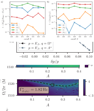
Figure 4: Dephasing rate $\Gamma_{\phi,ac}$ due to amplitude noise, along with the double sweet spot marked with $\circ$ and the amplitude dephasing rate $\Gamma_{\phi,ac}^{*}$ at that point. Although the qubit is linearly sensitive to amplitude fluctuations, those fluctuations are of very low amplitude in a good-quality signal generator, so the net dephasing impact is expected to be comparable to that from flux noise.

III.2 Depolarization from flux and charge noise

The computed bit flip rate due to flux and charge noise is shown in Figure 5(a).

For a static qubit, the decoherence rate associated to an operator $\mathcal{O}$ is modeled by Fermi’s golden rule

$$\widetilde{\Gamma}_{1\mathcal{O}}=\frac{1}{\hbar^{2}}\left|\braket{0}{\mathcal{O}}{1}\right|^{2}S_{\mathcal{O}}(\epsilon_{01})$$ (10)

where $S_{\mathcal{O}}$ is the spectral density of the noisy parameter coupled to $\mathcal{O}$. For the Floquet qubit, we must modify the formula to account for the time-dependence of the quasi-eigenstates as well as the ambiguity in the quasi-energies $\mathrm{mod}\,\Omega$. Instead we use

$$\Gamma_{1\mathcal{O}}=\frac{1}{\hbar^{2}}\sum_{k=-\infty}^{\infty}S_{\mathcal{O}}(\epsilon_{10}+k\Omega)\left|\overline{\braket{0}{\mathcal{O}e^{ik\Omega t}}{1}}\right|^{2}$$ (11)

where $\overline{(\dots)}$ denotes averaging over one period of the drive [24].

We define the total depolarization rate $\Gamma_{1}$ from capacitive and inductive loss by summing the individual $\Gamma_{1\mathcal{O}}$ over all $\mathcal{O}\in\{\varphi_{L},\varphi_{R},n_{L},n_{R}\}$, with spectral densities

$$S_{\varphi_{j}}(\omega)=\frac{2\hbar}{LQ_{ind}(\omega)}\frac{\coth\frac{\hbar|\omega|}{2k_{B}T}}{1+\exp\frac{-\hbar\omega}{k_{B}T}}$$ (12)

for a noisy inductance $L$ and

$$S_{n_{j}}(\omega)=\frac{2\hbar}{CQ_{cap}(\omega)}\frac{\coth\frac{\hbar|\omega|}{2k_{B}T}}{1+\exp\frac{-\hbar\omega}{k_{B}T}}$$ (13)

for a noisy capacitance $C$, at $T=15$mK, with assumed frequency-dependent quality factors of

$$Q_{ind}(\omega)=\left(500\times 10^{6}\right)\frac{K_{0}\left(\frac{h\times 0.5\textrm{ GHz}}{2k_{B}T}\right)\sinh\left(\frac{h\times 0.5\textrm{ GHz}}{2k_{B}T}\right)}{K_{0}\left(\frac{\hbar|\omega|}{2k_{B}T}\right)\sinh\left(\frac{\hbar|\omega|}{2k_{B}T}\right)}$$ (14)

for the inductor and

$$Q_{cap}(\omega)=10^{6}\times\left(\frac{6\textrm{ GHz}}{|\omega|/2\pi}\right)^{0.7}$$ (15)

for the capacitor [14].

By construction, the wavefunctions of the computational states $\psi_{0}=\braket{\bm{\varphi}}{0}$ and $\psi_{1}=\braket{\bm{\varphi}}{1}$ have nearly disjoint support at all times $t$. Thus their matrix element with respect to the error operators $\varphi_{C,D}$ are small, which reduces the rate of depolarization errors. By the same reasoning, transitions from the charge operator $n_{j}\propto\tfrac{\partial}{\partial\varphi_{j}}$ are also suppressed.

Figure 5: The depolarization $\Gamma_{1}$ error rate computed for the FFM qubit, with the double sweet spot marked with $\circ$ and the depolarization rate $\Gamma_{1}^{*}$ at that point. The erasure error rate is roughly constant at $\Gamma_{e}\approx 1.91$ kHz.

III.3 Erasure errors

Erasure errors, where a computational state decays to an erasure state, follow the same eq. (11) as bit flip errors, but involve different final quasi-eigenstates and thus different matrix elements. The erasure bit flip rate due to flux and charge noise is shown in Figure 5(b). These errors are much more likely to occur than bit flips in the FFM qubit because the relevant matrix elements $\braket{i}{\varphi_{j}}{E_{k}}$ between computational and leakage states are not engineered to be small like the bit-flip matrix elements. We predict that they are by far the dominant source of logical errors in the qubit, occurring at roughly the kHz level.

III.4 Shot noise

In order to perform dispersive readout operations on the qubit it must be coupled to an external resonator. Shot noise stems from uncertainty in the photon population in this readout resonator, which dephases the qubit due to the dispersive shift $\chi$. We discuss the dispersive shift in the context of qubit readout in Section IV.2, but here it affects the overall phase coherence through the shot noise rate

$$\Gamma_{\phi,\chi}=\frac{\overline{n}\kappa}{1+\kappa^{2}/\chi^{2}}$$ (16)

In this formula, $\overline{n}\ll 1$ is the expectation of the resonator photon number and $\kappa$ is the lifetime of the readout resonator [29]. The dispersive shift of our proposed device is roughly comparable to that of the (static) fluxonium molecule studied in [21], so we expect the shot noise estimates for the two devices to be comparable.

For our circuit parameters coupled to an 8 GHz readout resonator, we compute $\chi=0.65$ MHz (see section IV.2). Using $\overline{n}=10^{-4}$ and $\kappa=6$ MHz, we find $\Gamma_{\phi,\chi}=6.95$ Hz, which is comparable to the predicted dephasing from flux noise in the neighborhood of the double sweet spot.

IV Single-qubit gates and readout

We have shown that the FFM device has some ability to protect stored quantum information from decoherence. However, for practical use as a qubit, the device must be able to implement control and readout operations. In this section we show that single-qubit gates can be achieved to high fidelity with external polychromatic flux pulses. We also find that standard dispersive readout techniques can be used to measure the qubit.

Figure 6: Gate infidelity as a function of gate time for $X=R_{X}(\pi)$ and $Y=R_{Y}(\pi)$ gates induced by a secondary flux drive. The infidelity is minimized (solid lines) by optimizing the mix of secondary drive frequencies, achieving up to 4x faster gates at fixed $1-F$ compared to a simple unoptimized gate drive which is monochromatic at frequency $\Omega^{\prime}$ (dashed lines). For both $j=X$ and $Y$ gates, the primary gate axis coefficient satisfies $|c_{j}|^{2}>F-10^{-7}$. The dash-dotted black line indicates the probability of an erasure error occurring in any interval of length $t$ given the erasure rate from Table 2 and thus shows a control-independent lower-bound for uncorrected average gate fidelity. The inset shows optimized flux waveforms for the secondary gate flux drive of $\phi_{C}(\Omega^{\prime}t)$ and $\phi_{D}(\Omega^{\prime}t)$ (relative to the idle values $\phi_{C}=\pi$ and $\phi_{D}=2\pi A\cos\Omega^{\prime}t$) which implement an $X$ gate with $F=0.999$. Both insets are on the same axis scale. For this gate, the maximum drive amplitude is approximately $\alpha=A^{*}/744$ and the frequency offset is $\delta\Omega/2\pi=-137$ kHz.

IV.1 Single-qubit gates via additional flux drives

Single-qubit gates can be implemented with an additional drive of the external fluxes $\phi_{C,D}$ beyond the monochromatic drive of $\phi_{D}$ used to generate the Floquet physics of the qubit. During steady-state operation, the common flux is fixed at $\phi_{C}=\pi$ and $\phi_{D}$ is driven at frequency $\Omega$. To perform an $X$ or $Y$ gate, we must introduce another Hamiltonian term which mixes the computational states without coupling them too strongly to the erasure states or any other excited states of the circuit.

A gate drive using common mode flux, at the Floquet drive frequency $\Omega$, has a nonzero matrix element between the computational states and is thus used as a starting point for $R_{X}$ and $R_{Y}$ gates, from which one can generate all single-qubit gates. A bare drive of this form does not result in a high-fidelity gate, though, because its matrix elements with excited and erasure states are too large and result in significant leakage outside of the computational subspace. A weaker gate drive results in a higher-fidelity but much slower gate, and with a drive of this form we find that gate times of about 1 $\mu$s are required to reach 99.9% fidelity for $X$ and $Y$ gates.

We remedy the situation by introducing more drive tones of both $\phi_{C}$ and $\phi_{D}$ at higher harmonics of $\Omega$ and at $\pi/2$ phase offsets. This includes shifts of the drive amplitude $A$, and we also allow shifts of the base frequency $\Omega$. These additional tones can be made to cancel out much of the leakage from the computational subspace, increasing the gate fidelity at a fixed gate time.

Any gate Hamiltonian that approximately generates $X$- rotations in the computational basis has two eigenstates $\ket{\widetilde{+}}$ and $\ket{\widetilde{-}}$ that are approximate uniform superpositions of the computational states, with energy difference $\omega_{g}$. Evolution for time $t$ under this eigensystem produces the approximate rotation gate $R_{\bm{n}}(\omega_{g}t)$ around a Bloch sphere axis $\bm{n}$ determined by $\ket{\widetilde{+}}$ and $\ket{\widetilde{-}}$. To bound the gate fidelity for all $t$ in this rotation family, we define the basis change matrix $M_{ij}$ by $M_{ij}=\braket{i}{\widetilde{j}}$ with $i\in\{0,1\}$ and $j\in\{+,-\}$. $M$ is approximately unitary, but fails to be exactly unitary due to residual nonzero support of the gate eigenbasis on leakage and excited states. Under these conditions, we define the fidelity $F$ with respect to the computational basis:

$$F=\sum_{j\in\{x,y,z\}}|\operatorname{tr}M\sigma_{z}M^{\dagger}\sigma_{j}/2|^{2}=\sum_{j\in\{x,y,z\}}|c_{j}|^{2}$$ (17)

This defines the gate axis coefficients $c_{x,y,z}$. Note that the closest unitary gate being applied in this case corresponds to rotation around $\bm{n}=(c_{x},c_{y},c_{z})^{\top}$. The gate time required for an $X$ gate is then $t=\pi/\omega_{g}$.

An exactly analogous situation is the same for $Y$ rotations, except that the eigenstates $\ket{\widetilde{+y}}$ and $\ket{\widetilde{-y}}$ contain the required additional phase.

We determine the optimal mix of drive tones and frequency offset through optimization. We assume a gate Hamiltonian of the form

$$H_{gate}=H_{FFM}(A^{*},\Omega^{\prime})+\sum_{k=0}^{m_{g}}\,\sum_{j,\theta}x_{jk\theta}\,\varphi_{k}\cos\left(j\Omega^{\prime}t+\theta\right)$$ (18)

where $j\in\{C,D\}$, the phase is $\theta=0$ or $\pi/2$, and $\Omega^{\prime}=\Omega^{*}+\delta\Omega$. This Hamiltonian corresponds to time-dependent external fluxes with Fourier decompositions given by the $x_{jk\theta}$. To find the optimal $X$ gate parameters, for a range of initial amplitudes $A_{gate}$ we fix $x_{C10}=A_{gate}$ and then optimize over the remaining parameters $x_{jk\theta}$ and $\delta\Omega$ to maximize the axis coefficient $|c_{x}|$. For $Y$ the process is identical except that $x_{C1\tfrac{\pi}{2}}=A_{gate}$ is fixed instead and we maximize $|c_{y}|$. In practice, optimizing with a fixed $A_{gate}$ corresponds to different gate times even after the optimization is complete. For simplicity we only consider the few lowest Fourier modes by choosing $m_{g}=3$; we find that the fidelity is not significantly improved by increasing up to $m_{g}=5$.

The optimization results are shown in Figure 6 along with $\phi_{C}(\Omega t)$ and $\phi_{D}(\Omega t)$ waveforms for an $F=0.999$ $X$-type gate.

IV.2 Dispersive Readout

Standard dispersive readout methods employed for the static fluxonium molecule also apply unchanged to the FFM qubit. This is because the Floquet computational states have time-averaged wavefunctions similar to the static case, so that the inductive qubit-resonator interaction term

$$H_{int}=g(a+a^{\dagger})\varphi_{j}$$ (19)

(where $j=L$ or $R$) acts similarly in the two cases to generate the dispersive shift $\chi$. In particular, with $g=250$MHz we calculate a dispersive shift of $\chi=0.65$ MHz, compared to $\chi_{static}=0.47$ MHz. We also find that the dispersive shift between any computational state and any erasure states is of comparable magnitude and is $\geq 0.28$ MHz. Erasure errors are thus detectable during measurement of the qubit states without requiring a dramatic increase in the measurement sensitivity.

V Outlook

Figure 7: The double sweet spot exists for a wide range of circuit parameters. Here we show the fractional change in the sweet spot parameters $q$ (where $q\in\{\Omega^{*},A^{*}\}$) as a circuit parameter $p$ is adjusted from its value in Table 2. We use $p\in\{E_{L}^{\prime},E_{J}\}$ and cutoff values of $N=50$, $M=39$, and we computed the location of the double sweet spot through numerical optimization of the coherence time. The flux-noise dephasing rate remains low at each point, satisfying $\Gamma_{\phi,\varphi_{D}}+\Gamma_{\phi,\varphi_{C}}\leq 1$ Hz.

In summary, we have presented a novel type of superconducting qubit, the FFM qubit, which uses a strong flux drive to suppress dephasing while preserving a high $T_{1}$. The procedure unavoidably introduces two additional erasure states. For the circuit parameters that we have explored, the dephasing error rate is an order of magnitude less then the depolarizing error rate, which in turn is two orders of magnitude less then the erasure error rate. It might be possible to decrease both the depolarization and erasure error rates somewhat by further tuning circuit parameters. Additionally, the bias toward erasure errors is favorable for quantum error correction [9].

In addition to the coherence analysis, we have optimized waveforms for flux-driven single qubit rotation gates. We leave the implementation of multi-qubit gates to future work.

The existence of a double sweet spot is not unique to the circuit parameters in Table 2; indeed, the four-level coherence analysis in section II.2 relies only on the assumption that $E_{L},E_{C}\ll E_{J}$. We emphasize this point in Figure 7, which shows how the sweet spot parameters $A^{*},\Omega^{*}$ move as the two circuit parameters $E_{J}$ and $E_{L}^{\prime}$ are independently tuned.

Lastly, we point out that the design motivation may be more broadly applicable to other types of qubit hardware. The key ingredient to achieving the low error rates is enhanced tunneling between the two non-computational states of two coupled qubits that exhibit localized, disjoint eigenstates. This tunneling is obtained by selectively coupling them with a resonant drive, delocalizing them and lifting degeneracy with the still-disjoint computational states; the result is a non-divergent and even potentially vanishing $\Delta^{(2)}$. Although we have discussed a concrete implementation with fluxonium and circuit QED, this general formula could be applied to different physical systems of coupled qubits. Spin qubits in particular could be an attractive platform as their Hilbert space is finite-dimensional, avoiding the problem of multi-photon resonances from strong drives.

Appendix A The Floquet frequency lattice

In the following sections we will explain how to diagonalize the Floquet Hamiltonian $K_{4}$ of the FFM qubit considering the lowest four levels of the static Hamiltonian $H_{dc}$ only. In this case, $H_{dc}$ is equal to $H_{FFM}(t=0)$ with $A=0$, or equivalently eq. (2) with constant $\phi_{L}(t)=\phi_{R}(t)=\pi$.

The Floquet theorem [30] guarantees the existence of a set of states $\ket{\psi_{\alpha}(t)}$ of the following form that, at all times $t$, both form a complete basis of states and solve the Schrodinger equation:

$$\ket{\psi_{\alpha}(t)} =e^{-i\epsilon_{\alpha}t}\ket{q_{\alpha}(t)}$$ (20)

$$i\partial_{t}\ket{\psi_{\alpha}(t)} =H_{FFM}(t)\ket{\psi_{\alpha}(t)}$$ (21)

such that the states $\ket{q_{\alpha}(t)}$ are periodic with period $\tau=2\pi/\Omega$. These states are referred to as quasi-eigenstates and the $\epsilon_{\alpha}$ are known as quasi-energies; a consequence of the definition is that the $\epsilon_{\alpha}$ are only uniquely defined $\mathrm{mod}\,\Omega$.

An equivalent formulation, known as the frequency lattice, defines a new Hermitian operator $K$ over a larger Hilbert space and encodes the quasi-eigenstates and -energies in its eigenvectors and eigenvalues. As the $\ket{q_{\alpha}}$ are periodic, we may Fourier-expand them:

$$\ket{q_{\alpha}(t)}=\sum_{n=-\infty}^{\infty}e^{in\Omega t}\ket{\phi_{n\alpha}}$$ (22)

where the Fourier components $\ket{\phi_{n\alpha}}$ are un-normalized. Similarly we denote the $n$-th Fourier component of $H_{FFM}$ as $\widetilde{H}_{n}$. Then, integrating the Schrodinger equation over one period yields an eigenvalue equation for the $\ket{\phi_{j\alpha}}$:

$$K_{ij} =\widetilde{H}_{i-j}+j\Omega\delta_{ij}$$ (23)

$$\left(\bm{\phi}_{\alpha}\right)_{j} =\ket{\phi_{j\alpha}}$$ (24)

$$\epsilon_{\alpha}\bm{\phi}_{\alpha} =K\cdot\bm{\phi}_{\alpha}$$ (25)

Here, we have defined the Floquet Hamiltonian $K$, which is a block matrix: the blocks are labeled by the Fourier indices $(i,j)$, and within a block the matrix acts on the Hilbert space of $H_{dc}$. We will find the time-dependent quasi-eigenstates by solving for their Fourier expansions, the eigenvectors $\bm{\phi}_{\alpha}$ of $K$.

Appendix B Diagonalizing $K_{FFM}$

We now proceed with analyzing $H_{FFM}$, with $\phi_{D}(t)=2\pi A\cos\Omega t$ and $\phi_{C}=\pi$. By the Floquet theorem, this has identical quasi-energies to the alternative phase choice of $\phi_{D}\propto\sin\Omega t$, although the quasi-eigenstates will carry different phases. This choice of $H_{FFM}$ has the following Fourier components:

$$\widetilde{H}_{k}=\begin{cases}H_{dc}&k=0\\ \tfrac{A\pi}{4}\Delta E\,\varphi_{D}&|k|=1\\ \tfrac{A^{2}\pi^{2}}{8}\Delta E&|k|=2\\ 0&|k|>2\end{cases}$$ (26)

Here, $A$ is the differential flux drive amplitude and $\Delta E=2E_{L}-E^{\prime}_{L}$. We will project to the subspace $\mathcal{H}_{4}$ spanned by the four lowest eigenstates of $H_{dc}$, labeled $g,e,h,f$ with energies $0,\delta,\Delta,\mu$ respectively. In this basis $B^{\prime}$ we have the matrices

$$(H_{dc})_{B^{\prime}} =\left(\begin{array}[]{cccc}0&&&\\ &\delta&&\\ &&\Delta&\\ &&&\mu\\ \end{array}\right)$$ (31)

$$(\varphi_{D})_{B^{\prime}} =\varphi_{0}\left(\begin{array}[]{cccc}0&1&0&0\\ 1&0&-\sqrt{2}\epsilon&0\\ 0&-\sqrt{2}\epsilon&0&0\\ 0&0&0&0\\ \end{array}\right)$$ (36)

Equation (36) defines the parameters $\varphi_{0}$ and $\epsilon$, and we will assume that $\epsilon$ is small in order to use it as a perturbative parameter. For the parameters in Table 2 we compute $\epsilon=0.0437$.

It will be more convenient to work in an eigenbasis of $\varphi_{D}$ restricted to $\mathcal{H}_{4}$. We label these states $x,y,z,w$, and in this basis $B$ we obtain the following matrices:

$$(\varphi_{D})_{B} =\varphi_{0}\left(\begin{array}[]{cccc}-\sqrt{1+2\epsilon^{2}}&&&\\ &\sqrt{1+2\epsilon^{2}}&&\\ &&0&\\ &&&0\\ \end{array}\right)$$ (41)

$$(H_{dc})_{B} =\Delta\left(\begin{array}[]{cccc}\epsilon^{2}+\frac{r}{2}&\epsilon^{2}-\frac{r}{2}&-\epsilon&0\\ \epsilon^{2}-\frac{r}{2}&\epsilon^{2}+\frac{r}{2}&-\epsilon&0\\ -\epsilon&-\epsilon&1-2\epsilon^{2}&0\\ 0&0&0&\mu/\Delta\\ \end{array}\right)$$ (46)

Here we have put $r=\delta/\Delta$. Notice that the $f$ state was decoupled from the other rows of the $\varphi_{D}$ matrix in equation (36), so we have taken $\ket{w}=\ket{f}$.

This is a desirable situation, as we can now do perturbation theory in $\epsilon$ and $r$. All terms of order zero in these parameters are on the diagonal of both $H_{dc}$ and $\varphi_{D}$, which means that the zeroth order Floquet Hamiltonian $K^{(0)}$ is exactly solvable. In fact it is the direct sum of two infinite 5-diagonal matrices $X$ and $Y$ as well as two infinite tri-diagonal matrices $Z$ and $W$:

$$X_{ij}=-z_{0}\Omega(\delta_{i,j-1}+\delta_{i,j+1})+z_{1}\Omega(\delta_{i,j-2}+\delta_{i,j+2})+j\Omega\delta_{ij}$$ (47)

$$Y_{ij}=z_{0}\Omega(\delta_{i,j-1}+\delta_{i,j+1})+z_{1}\Omega(\delta_{i,j-2}+\delta_{i,j+2})+j\Omega\delta_{ij}$$ (48)

$$Z_{ij}=z_{1}\Omega(\delta_{i,j-2}+\delta_{i,j+2})+(j\Omega+\Delta)\delta_{ij}$$ (49)

$$W_{ij}=z_{1}\Omega(\delta_{i,j-2}+\delta_{i,j+2})+(j\Omega+\mu)\delta_{ij}$$ (50)

where the indices $i,j$ range over all integers. We have introduced the normalized drive amplitudes $z_{0}=A/A_{0}$ and $z_{1}=(A/A_{1})^{2}$ with

$$1/A_{0} =\frac{\pi\varphi_{0}\sqrt{1+2\epsilon^{2}}}{2}\frac{\Delta E}{\Omega}$$ (51)

$$1/A_{1}^{2} =\frac{\pi^{2}\varphi_{0}}{4}\frac{\Delta E}{\Omega}$$ (52)

The diagonalizations of these matrices are known. In each case, the eigenvalues are the diagonal entries: for each integer $n$, they are $n\Omega$ for $X$ and $Y$, $n\Omega+\Delta$ for $Z$, and $n\Omega+\mu$ for $W$. The eigenvector labeled by the integer $n$, denoted by the corresponding lowercase letter (for instance, $\ket{\widetilde{x},n}$ for the $X$ matrix), is, for each of the four matrices,

$$\ket{\widetilde{x},n} =\sum_{k=-\infty}^{\infty}\sum_{m=-\infty}^{\infty}J_{m}(z_{1})J_{k-n-2m}(-z_{0})\ket{x,k}$$ (53)

$$\ket{\widetilde{y},n} =\sum_{k=-\infty}^{\infty}\sum_{m=-\infty}^{\infty}J_{m}(z_{1})J_{k-n-2m}(z_{0})\ket{y,k}$$ (54)

$$\ket{\widetilde{z},n} =\sum_{m=-\infty}^{\infty}J_{m}(z_{1})\ket{z,2m+n}$$ (55)

$$\ket{\widetilde{w},n} =\sum_{m=-\infty}^{\infty}J_{m}(z_{1})\ket{w,2m+n}$$ (56)

where for instance $\{\ket{x,n}\}_{n\in\mathbf{Z}}$ labels the standard basis of the matrix $X$ and so on for $Y,Z,W$. Since $K^{(0)}=X\oplus Y\oplus Z\oplus W$, these four collections of states together constitute an eigenbasis for $K^{(0)}$.

At this point we will make the assumption that $\Omega\approx\Delta$, which means that for each integer $n$ (at order zero in $\epsilon$ and $r$) there is a triplet of nearly degenerate states: in particular, $S_{n}=\operatorname{span}\{\ket{\widetilde{x},n},\ket{\widetilde{y},n},\ket{\widetilde{z},n-1}\}$ is a nearly degenerate subspace under $K^{(0)}$. Additionally, the $W$ eigenstates have all zero matrix elements with the $r$ and $\epsilon$ perturbations, so we are finished with them for now and will restrict our attention to the $S_{n}$ subspaces. In particular, we use the Generalized Van Vleck (GVV) formalism to perform nearly-degenerate perturbation theory in each subspace.

As a simplifying assumption, we will work only in one perturbative parameter $\epsilon$ by setting $r=R\epsilon^{2}$ with $R$ fixed. In principle this is not necessary for the GVV formalism, but the assumption is valid for a wide range of device parameters, including the ones we consider numerically, and can if necessary be lifted on a case-by-case basis. For our parameters $R=1.148$.

According to the GVV formalism [31], we form the effective Hamiltonian matrix up to order $\epsilon^{2}$, along with the basis vectors $\mathbf{b}_{j}$ ($j=1,2,3$) up to order $\epsilon$:

$$G =\sum_{m}\epsilon^{m}G^{(m)}$$ (57)

$$\bm{b}_{j} =\sum_{m}\epsilon^{m}\bm{b}_{j}^{(m)}$$ (58)

$$\bm{b}^{(0)} =\begin{pmatrix}\ket{\widetilde{x},n}&\\ \ket{\widetilde{y},n}&\\ \ket{\widetilde{z},n-1}&\end{pmatrix}$$ (59)

The relevent higher-order terms are

$$\bm{b}_{j}^{(1)} =R_{j}K^{(1)}\cdot\bm{b}_{j}^{(0)}$$ (60)

$$G^{(0)} =\bm{b}^{(0)}\cdot K^{(0)}\cdot\bm{b}^{(0)}$$ (61)

$$G^{(1)} =\bm{b}^{(0)}\cdot K^{(1)}\cdot\bm{b}^{(0)}$$ (62)

$$G^{(2)} =\bm{b}^{(0)}\cdot K^{(2)}\cdot\bm{b}^{(0)}+\bm{b}^{(0)}\cdot K^{(1)}\cdot\bm{b}^{(1)}-G^{(1)}\cdot\left(\bm{b}^{(0)}\bm{b}^{(1)}\right)$$ (63)

where $R_{j}=\sum_{\phi}\frac{\ket{\phi}\bra{\phi}}{E_{j}-E_{\phi}}$ is the resolvent.

However, we will ultimately be interested in a low-amplitude regime. By working to zeroth order in $z_{1}\propto A^{2}/32$, we can simplify the algebra considerably.

Appendix C Low-amplitude approximation

To simplify the analysis we will now make the approximation of $z_{1}\ll 1$. Working to zeroth order in $z_{1}$, the states in $S_{n}$ are simplified:

$$\ket{\widetilde{x},n} =\sum_{k=-\infty}^{\infty}J_{k-n}(-z_{0})\ket{x,k}$$ (64)

$$\ket{\widetilde{y},n} =\sum_{k=-\infty}^{\infty}J_{k-n}(z_{0})\ket{y,k}$$ (65)

$$\ket{\widetilde{z},n} =\ket{z,n}$$ (66)

$$\ket{\widetilde{w},n} =\ket{w,n}$$ (67)

Using this, the $G^{(k)}$ matrices can be computed for each integer $n$:

$$G^{(0)} =\left(\begin{array}[]{ccc}n\Omega&0&0\\ 0&n\Omega&0\\ 0&0&\Delta+(n-1)\Omega\\ \end{array}\right)$$ (71)

$$G^{(1)} =\Delta J_{1}(z_{0})\left(\begin{array}[]{ccc}0&0&1\\ 0&0&-1\\ 1&-1&0\\ \end{array}\right)$$ (75)

$$G^{(2)} =\Delta\left(\begin{array}[]{ccc}\left(\frac{R}{2}+1\right)+\ f_{-}&\left(1-\frac{R}{2}\right)J_{0}(2z_{0})+f_{+}&0\\ \left(1-\frac{R}{2}\right)J_{0}(2z_{0})+f_{+}&\left(\frac{R}{2}+1\right)+f_{-}&0\\ 0&0&-2(1+f_{-})\\ \end{array}\right)$$ (79)

The functions $f_{+}$ and $f_{-}$ are defined as

$$f_{\pm}=-\sum_{k\neq 0}\frac{J_{1-k}(z_{0})J_{k-1}(\pm z_{0})}{k}$$ (80)

The eigenvectors of $G^{(\leq 2)}=G^{(0)}+\epsilon G^{(1)}+\epsilon^{2}G^{(2)}$ are

$$\bm{e}_{0} =\frac{1}{\sqrt{2}}\begin{pmatrix}1&1&0\end{pmatrix}^{\top}$$ (81)

$$\bm{e}_{1} =\frac{1}{\mathcal{N}_{1}}\begin{pmatrix}(\alpha_{1}-\alpha_{2})&(\alpha_{2}-\alpha_{1})&1\end{pmatrix}^{\top}$$ (82)

$$\bm{e}_{2} =\frac{1}{\mathcal{N}_{2}}\begin{pmatrix}(\alpha_{1}+\alpha_{2})&(-\alpha_{1}-\alpha_{2})&1\end{pmatrix}^{\top}$$ (83)

$$\alpha_{1} =\frac{\epsilon\big{(}(R-2)J_{0}(2z_{0})+R+2(3f_{-}-f_{+}+3)\big{)}+2\epsilon^{-1}(\Omega/\Delta-1)}{8J_{1}(z_{0})}$$ (84)

$$\alpha_{2} =\sqrt{\alpha_{1}^{2}+\frac{1}{2}}$$ (85)

Here $\mathcal{N}_{1}$ and $\mathcal{N}_{2}$ are normalizations fixed by $\|\bm{e}_{j}\|=1$. We choose the state corresponding to $\bm{e}_{0}$ (with $n=1$) to be the computational state $\ket{0}$, and the $\ket{w,0}$ state to be the computational state $\ket{1}$. The other two states corresponding to $\bm{e}_{1}$ and $\bm{e}_{2}$ are then the erasure states.

The $\ket{0}$ computational state is

$$\ket{0}=\frac{1}{\sqrt{2}}\left(\ket{\widetilde{x},0}+\ket{\widetilde{y},0}\right)+O(\epsilon)$$ (86)

As we now have expressions for the erasure states, we can compute their matrix elements with respect to $\varphi_{C}$ and $\varphi_{D}$, and thus calculate the second-order dephasing contribution $\Delta^{(2)}$. We find the following conditions on $\Omega^{*j}$, the drive frequency where $\Delta^{(2)}_{j}=0$ for $j=\varphi_{D}$ or $j=\varphi_{C}$ respectively:

$$\Omega^{*D} =\Delta-\Delta\epsilon^{2}\left(3+3f_{-}+f_{+}+\tfrac{R}{2}+J_{0}(2z_{0})(1-\tfrac{R}{2}))\right)$$ (87)

$$\Omega^{*C} =\mu-\Delta\epsilon^{2}\left(1+f_{-}-f_{+}+\tfrac{R}{2}-J_{0}(2z_{0})(1-\tfrac{R}{2})\right)$$ (88)

These curves in the $(z_{0},\Omega)$ plane may cross zero or more times depending on the parameters $R$ and $\Delta-\mu$. If it exists, we denote the point at which they cross with minimal $z_{0}$ as $(z_{0}^{*},\Omega^{*})$ which through equation (51) gives $(A^{*},\Omega^{*})$.

The qubit frequency is given by

$$\epsilon_{10}=\mu-\Omega-\Delta\epsilon^{2}\left(1+f_{-}+f_{+}+\tfrac{R}{2}+J_{0}(2z_{0})(1-\tfrac{R}{2})\right)$$ (89)

Appendix D Numerical simulation convergence

Figure 8: Convergence of our numerical simulations, showing the (a) relative quasi-energy change and (b) change in the overlap of the quasi-eigenstates as the static cutoff $N$ is tuned from its nominal value of $300$. The Fourier cutoff of the quasi-eigenstates (which are exponentially localized in Fourier space) is fixed at $M=63$. The largely independent and small differences as a function of the static cutoff indicate that the simulation results at $N=300$ are relatively well converged.

The wavefunctions and coherence data in Figures 1-3, 5, and 6 are the result of numerical diagonalization of the Floquet frequency lattice Hamiltonian $K$ (see Appendix A) with $M=63$ Fourier modes (ranging from $-31$ to $31$) and the lowest $N=300$ eigenstates of the static $H_{FM}$. Figure 6 instead used $N=400$ static eigenstates. In all cases eigenstates of $H_{FM}$ were obtained by diagonalizing eq. (2) with $\phi_{C}=\pi$ and $\phi_{D}=0$ in the harmonic oscillator basis where $\phi_{L,R}=\frac{x_{0}}{\sqrt{2}}(a_{L,R}+a_{L,R}^{\dagger})$, with $x_{0}=\sqrt[4]{8E_{C}/E_{L}}$, using 100 basis states each of $a_{L}$ and $a_{R}$ for a total of $10^{5}$ ladder operator basis states.

We provide evidence that our simulation of the computational and erasure states is converged in Figure 8 where we tune the static cutoff $N$ from 300 to 475. The Fourier cutoff is fixed at $M=63$, which we expect provides a good approximation due to exponential Wannier-Stark localization in the frequency lattice [32].