DiscoTEX: Discontinuous collocation and implicit-turned-explicit (IMTEX) integration symplectic, symmetric numerical algorithms with higher order jumps for differential equations with numerical black hole perturbation theory applications

Abstract

Dirac $\delta-$distributionally-sourced differential equations emerge in many dynamical physical systems from machine learning, finance, neuroscience, seismology to black hole perturbation theory. Most of these systems lack exact analytical solutions and are thus best tackled numerically. In this work, one describes a generic numerical algorithm which constructs discontinuous spatial and temporal discretisations by operating on discontinuous Lagrange and Hermite interpolation formulae recovering higher order accuracy. One demonstrates, by solving the distributionally sourced wave equation which possesses analytical solutions, that numerical weak-form solutions can be recovered to high order accuracy by solving a first-order reduced system of ordinary differential equations. The method-of-lines framework is applied to the DiscoTEX algorithm i.e through discontinuous collocation with implicit-turned-explicit IMTEX integration methods which are symmetric and conserve symplectic structure. Furthermore, the main application of the algorithm is proved, for the first-time, by calculating the amplitude at any desired location within the numerical grid, including at the position (and at its right and left limit) where the wave- (or wave-like) equation is discontinuous via interpolation using the DiscoTEX algorithm. This is demonstrated, firstly by solving the wave- (or wave-like) equation and comparing the numerical weak-form solution to the exact solution. Finally, one demonstrates how to reconstruct the scalar and gravitational metric perturbations from weak-form numerical solutions of a non-rotating black hole which do not have known exact analytical solutions and compare against known state-of-the-art frequency domain results. One concludes by motivating how DiscoTEX, and related numerical algorithms, open a promising new alternative Extreme-Mass-Ratio-Inspiral (EMRI)s waveform generation route via a self-consistent evolution for the black hole perturbation theory gravitational self-force programme in the time-domain.

organization=School of Mathematical Sciences, Queen Mary University of London, city=London, postcode=E1 4NS, country=UK

1 Introduction

Dirac $\delta-$distributionally-sourced wave and (wave-like) equations are present in many dynamical systems from machine learning [1], finance [2], neuroscience [3, 4, 5, 6], seismology [7, 8, 9], probability [10, 11] to gravitational physics [12, 13, 14, 15, 16]. In this work a new algorithm will be presented with application to gravitational physics and designed to optimally address the difficulties faced by previous numerical methods applied within the radiation-reaction community when modelling Extreme-Mass-Ratio-Inspirals (EMRIs). These systems governing field equations describe the binary motion of a massive black hole (BH), of mass $M$, orbited by a much smaller compact object a black hole, of mass $\mu$, or neutron-star. The significant mass discrepancy naturally leads to a perturbative treatment, through the black hole perturbation theory (BHPT) machinery, where the binary motion is systematically expanded in terms of the ratio between the two bodies’ masses, $\epsilon=\mu/M$. The smaller BH is approximated as a point-particle where at zeroth-order in $\mu$ it follows the geodesic of the massive BH background, at first-order it deviates from the geodesic due to the interaction with its self-field. This deviation from its self-field is the self-force. The metric is perturbed as,

$$g^{\textrm{Exact}}_{\alpha\beta}=\bar{g}_{\alpha\beta}+\epsilon h^{(1)}_{\alpha\beta}+\epsilon^{2}h^{(2)}_{\alpha\beta}+\mathcal{O}(\epsilon^{3}),$$ (1)

where the bar notation denotes the metric given with respect to the background BH. Extensive theoretical work [17] has shown that expansions are only necessary up to second-order for accurate EMRI waveform models [16, 18]. The starting point in numerical BHPT is expanding the linearized Einstein equations,

$$G_{\alpha\beta}=\frac{8\pi G}{c^{4}},$$ (2)

to the required orders, in this work the focus is on expansions up to first-order given as,

$$G_{\alpha\beta}=\bar{G}_{\alpha\beta}+\delta G_{\alpha\beta}/2,$$ (3)

$$\delta G_{\alpha\beta}=\frac{16\pi G}{c^{4}}T_{\alpha\beta}.$$ (4)

To note here, going from the first to second line, $\bar{G}_{\alpha\beta}=0$, because the background BHs under study are solutions to the Einstein vacuum equations, specifically here the focus is on a Schwarzschild BH background. The tensor, $T_{\alpha\beta}$, is the external matter perturbing the background BH written in terms of Dirac $\delta-$distributions reflecting the point-particle model of the compact object in BHPT,

$$T_{\alpha\beta}=\mu\int^{\infty}_{\infty}\frac{u_{\alpha}u_{\beta}}{\sqrt{-g}}\delta^{4}(x^{\alpha}-z^{\alpha}(s))\ ds$$

$$=\mu\frac{u_{\alpha}u_{\beta}}{u^{t}r_{p}(t)^{2}}\delta(r-r_{p}(t))\delta(\theta-\theta_{p}(t))\delta(\phi-\phi_{p}(t)).$$ (5)

where $s$ is the particle’s proper time, the point-particle moves on a geodesic with worldline $z^{\alpha}(s)$ and the four velocity is defined by $u^{\alpha}=dz^{\alpha}/ds$. The natural next step to the numerical BH perturbation theorist is to take advantage of the spherically symmetry of the Schwarzschild background and re-writing $h_{\alpha\beta}$ as a composition of radial and angular dependencies decomposed into a basis of spherical harmonics. Generically one writes,

$$h_{\alpha\beta}(t,r,\theta,\phi)=\sum^{\infty}_{a}\sum_{lm}h^{a,lm}(t,r)(\textbf{t}^{a,lm})_{\alpha\beta}(\theta,\phi)$$ (6)

where $a=\{L0,T0,E1,E2,B1,B2,tt,Rt,Et,Et,Bt\}$ [19, 20]. The perturbations equations in Eq.(4) can then be obtained by varying the Einstein tensor, which in the Regge-Wheeler [21, 22, 23, 19, 20] (or radiation gauges [24, 25, 26, 27]) simplifies to a partial-differential-equation of the type

$$\bigg{[}-\frac{\partial^{2}}{\partial t^{2}}+\frac{\partial^{2}}{\partial x^{2}}-V_{l}(r)\bigg{]}\Psi(t,r)=\square\Psi(t,r)=S_{lm}(t,r)$$

$$=F(t,r)\delta(r-r_{p})+G(t,r)\delta^{\prime}(r-r_{p}),$$ (7)

where $x$ is the tortoise coordinate, $x=r+2M\log(r/2M-1)$, $V_{l}(r)$ is some potential remaining from the harmonic decomposition of the background Schwarzschild’s or Kerr’s backgrounds and $S_{lm}(t,r)$ describes the source term emerging from the scalar or gravitational perturbations. The numerical recipe for the necessary gravitational self-force (GSF) computations can then be summarised in three main phases: Phase 1 - requires one to accurately solve for the master functions $\Psi(t,r)$ in the PDE in Eq.(7); Phase 2 - uses the numerical solution to reconstruct the metric perturbations as described by Eq.(1) and finally Phase 3 - uses the amplitudes of the metric perturbations to compute the gravitational self-force. As it stands it is highly unlikely that equations such Eq.(7) possess exact known analytical solutions [16], one must therefore resort to numerical approaches. Given the distributional nature of Eq.(7) a jump discontinuity arises at the point-particle location, $r=r_{p}(t)$, the strategy here is to let Eq.(7),

$$\Psi(t,r)=\Psi^{+}(t,r)\Theta[r-r_{p}(t)]+\Psi^{-}(t,r)\Theta[r_{p}(t)-r],$$ (8)

admit weak-form solution to the inhomogenous master functions $\Psi(t,r)$ [28, 23, 29]. Here the $\Psi^{+/-}$ are extensions of the smooth, homogeneous solutions of $\Psi(t,r)$ in Eq.(7) as they approach the particle position from the right and left, respectively, and $\Theta[r-r_{p}(t)]$ is the Heaviside step-function. As it has been shown by [23, 29] one can then re-write the metric perturbations in Eq.(1) in functional form as

$$h(t,r)=h^{+}(t,r)\Theta[r-r_{p}(t)]+h^{-}(t,r)\Theta[r_{p}(t)-r]$$

$$+h^{S}(t)\delta(r-r_{p}(t)),$$ (9)

where $h^{+/-}(t,r)$ represents a smooth function in the region around the particle $(r>r_{p}/r<r_{p})$ and $h^{S}(t)$ is a smooth function only time-dependent as demonstrated by [23] which gives the magnitude of the singularity. Schematically, Phase 3, numerically simply amounts to using Eq.(9) to compute the gravitational self-force as

$$\mathcal{F}^{\alpha,lm}_{\rm{ret}}=\lim_{r\rightarrow r_{p}^{\pm}}\sum^{m}_{l=-m}Y_{lm}(\theta,\phi)\int^{2\pi}_{0}\int^{\pi}_{0}\mathcal{F}^{\alpha}[\textbf{h}]Y^{*}(\theta^{\prime},\phi^{\prime})d\Omega^{\prime},$$ (10)

where this has been loosely defined. For a through regularised presentation please refer to state-of-the-art machinery of [20]. Given the physical requirements from black hole perturbation theory and the gravitational self-force programme, it is clear one must pick a:

• $[\texttt{REQ 1}]$: Suitable numerical solver - be able to produce an highly accurate numerical solution to distributional wave-like equations of the type Eq.(7) on any discretised spatial grid and time chart;

• $[\texttt{REQ 2}]$: Suitable “interpolator” - from the numerical solution in [REQ 1], one must be able to accurately compute the amplitude of the metric perturbation at the particle/smaller BH (i.e discontinuity, $r_{p}$) location and in its neighbourhood/limit as radiation propagates towards the horizon/infinity.

Numerical Integrator	Integrator type	Energy conservation	Symplectic	Symmetric	Stability
Traditional RK	EX	yes, numerically	partial, numerically	no	CFL constrained
[30, 31, 32, 33, 34, 35]
Gauss-Legendre RK	IM	yes, numerically	yes	yes	long-term stability
[36, 37]		long-term
Mixed RK	IMEX	yes, numerically	yes	no	long-term stability
[38, 39]		long-term
Horner-Form RK	EX	yes, numerically	partial, numerically	no	CFL constrained
“Slimplectic”	IM	yes, numerically	yes, but	yes	long-term stability
[40]		long-term
Mixed symplectic	IMEX	yes	yes	no	long-term stability
[41, 42, 43]
Traditional CN	IM	yes, numerically	yes, numerically	no	CFL constrained
[44]
IMTEX SCI ICN	IMTEX	yes, numerically	yes, numerically	no	CFL constrained
[45, 46, 47]
Hermite	IM	yes	yes	yes	unconditionally stable
[48, 49]
Hermite IMTEX	IMTEX	yes	yes	yes
Spectral SDIRK	IM	yes	yes	-	unconditionally stable
[50]

Table 1: Quick overview of different time-integrator schemes considered in this manuscript. Highlighted in pink are the integration schemes used in this work, and in orange one highlights upcoming work using different time-integrators.

As we reviewed in [49] there are four main difficulties associated with numerically solving these equations to accurately capture the orbital motion of EMRIs:

• Difficulty $(1)$ - how to treat the distributional source emerging from the point-particle model of the small BH; Numerically this means how can one resolve for the distributional nature of the problem in both the space and time dimension;

• Difficulty $(2)$ - what boundary conditions to impose such that radiation can be accurately extracted at the background BH limits;

• Difficulty$(3)$ - time-integrators must ensure highly accurate long-term simulations that can maintain sufficient accuracy for signals potentially lasting the entire 3 $\pm$ year LISA mission;

• Difficulty $(4)$ - how to choose initial conditions and understand their effect in the full radiative process.

In this work the focus will be mostly on difficulty $(1)$ and $(3)$. Difficulty $(2)$ amounts to a coordinate chart transformation of the problem in question with minimal changes to difficulties $(1,3)$. In Table 8 all the previous numerical methods used, to this author’s knowledge, within the radiation-reaction community are reviewed. The aim is to address important numerical algorithm details that were out of the scope of [49]. For difficult $(1)$ one will use discontinuous collocation methods to represent the Dirac $\delta$ distribution. These were initially introduced by [52] and further refined to the hyperboloidal wave equation and generic cases by [53, 54, 46]. Here, given one knows the local structure of the discontinuity at the point-particle a priori, we can adapt the Lagrange interpolation scheme by adding these known amplitudes, such that it holds for the case where the problem is smooth everywhere except at the point-particle’s location. Here, one will demonstrate how these can be numerically optimised for any function in both space and time. For spatial discontinuous discretisations, both finite-difference and pseudospectral methods will be considered generically against exact functions, one will then determine the necessary optimal factors associated with these; for functions that are discontinuous in time it is shown how we can incorporate discontinuities through Hermite interpolation formulae at higher orders, where one considers all orders (from $2^{nd}$ to $12^{th}$), demonstrating orders $6^{th}$ to $12^{th}$ for the first-time and justify our choices in [49]. Please refer to the first column of Table 8 for alternative solutions implemented by the community to resolve this difficulty.

EX explicit time-integration methods have been the standard choice when handling difficulty $(3)$, particularly the implementation of the Runge-Kutta, RK, order-four algorithm [55, 56]. This scheme not only results in an $n^{th}+1$ order error it is also riddled with errors from the real dynamical quantities, in its common EX RK form it does not preserve sympletic structure neither time-symmetry, energy is conserved with unbounded error numerically, and it also limited by a Courant-Friedrichs-Lewy (CFL) condition (i.e a limitation on the time discretization with respect to the spatial grid which ensures the numerical algorithm’s velocity does not surpass the physical velocity). These errors can usually be mitigated by further increasing the order of the algorithm [30, 31, 32, 33, 34] at the cost of increasing its complexity or by using adaptive step control [35] which is more computationally expensive. IM implicit methods on the other hand are unconditionally stable allowing for larger step-sizes and thus suitable for physical problems which have long-term evolutions, as the case of EMRIs. A well-known example of these schemes is the Crank-Nicholson (CN) integrator [44], which proved difficult to implement due to the complexity of the resulting algebraic equations. One solution came from Choptuik who suggested solving the CN scheme by self-consistent iterations (SCI) effectively turning it into an explicit scheme. To this author, within the numerical relativity community this was the first instance, where an implicit-turned-explicit, here called IMTEX, scheme was considered. However in the past, when attempting to use these IMTEX ICN scheme it was expected that iterating more than twice would not lead to improvements in both accuracy and stability [45], however, whereas the latter statement holds, as we showed in [46, 57, 47] accuracy, symmetry, sympletic structure preservation and energy conservation can be recovered with increasing number of iterations. This results is the key motivation to introducing the term IMTEX in [49, 47] as even though, while effectively explicit, for the IMTEX ICN scheme case it can preserve proprieties which were associated with the implicit scheme from which they are derived, and that should be kept in mind while implementing and studying its proprieties. Given the benefits of implicit schemes there have been significant efforts towards for example adapting the Runge-Kutta scheme to its IMEX form showing significant improvements in stability and long-term numerical energy conservation [38, 39]. Symplectic integrators [56] are characterised by exact preservation of sympletic structure, i.e the phase-space trajectories and volume is conserved resulting in long-term stability and bounded energy conservation. One recent example of are the completely sympletic scheme based on the implicit midpoint rule for conservative [58] and non-conservative [40] systems. Furthermore, recently mixed sympletic IMEX integrators have been explored [41, 42, 43]. In this work difficulty $(3)$ will be handled by using both implicit and the implicit-turned-explicit IMTEX Hermite integration schemes derived from implicit IM Hermite integration methods which show long-term stability, are energy-preserving, symmetric (that is they are both time-symmetric and $\rho-$ reversible) and preserve symplectic structure. This was partially demonstrated by this author in [48]. One will present results in optimised Horner-form and up to the $12^{th}$ order, justifying the choices used in previous and ongoing gravitational physics work [49]. Additionally, to highlight the singular proprieties IMTEX possesses and distinguish from schemes which are exclusively explicit EX one will compare its results to Runge-Kutta schemes which have also been written in optimal Horner-form. It will shown to achieve comparable accuracies even to the lowest $2^{nd}$ order IMTEX Hermite scheme one needs to go as far as $7^{th}$ orders with the EX RK scheme. Finally, one complements these results with an explicit proof showing in B.3 that our IMTEX Hermite integration schemes conserve exactly and numerically sympletic structure and energy, while being symmetric. In Table 8 column 4, entitled “Difficulty 3”, the numerical time-steppers used by the EMRI radiation reaction community can be found, the vast majority of the implementations were conditionally stable and hence minimised the chances of a successful long-term EMRI evolution.

Finally difficulty $(2)$ will be studied first by implementing radiation boundary conditions as previously done by [28, 52], followed by implementing an hyperboloidal slice [59, 60, 61, 62] as an alternative framework that ensures the governing equation automatically enforce outflow at the boundaries. Here the spacetime is parameterised by a compact radial coordinate defined on a hyperboloidal time hypersurface, allowing for measurements directly at the BH horizon and future null infinity. In this work the hyperboloidal slice know as the minimal gauge developed by [63, 64, 65, 66, 67] is used.

Altogether one will demonstrate how to solve both wave and (wave-like) equations as given in Eq.(7) through the means of the method-of-lines recipe by using the DiscoTEX algorithm: one implements discontinuous collocation methods to resolve the distributional point-source in both space and time direction and then integrate in time with an Hermite based IMTEX numerical method, effectively resolving difficulty $(3)$. Furthermore, these numerical weak-form solutions will be used to obtain the required reconstructed metric amplitudes through generic discontinuous interpolation formula possible via DiscoTEX. DiscoTEX’s validity will be verified firstly against the results obtained via exact known solutions of the wave equation [28, 68, 69] this allows one to prove and validate the algorithm.

The paper is organised as follows. In Section 2 one reviews the distributionally source wave-equation by highlighting the proprieties of both their exact solutions, as originally derived by Field [28, 68, 69], and their weak-form solutions [28, 68, 23]. In Section 3 it will be explained, on a step-by-step fashion, all the ingredients that make up DiscoTEX algorithm, and related algorithms, and explain the numerical optimisation factors necessary for an accurate implementation. This will be done by computing the solution to both the homogeneous and distributional sourced wave-like equation and by directly comparing against its exact solution. Three different types of wave-like equations, as derived by Field [28, 68, 69], are studied in exact and weak-form. In Section 4 one will demonstrate DiscoTEX’s applicability to numerical BHPT by solving the equations governing both the scalar and gravitational perturbations by a point-particle on a circular geodesic in Schwarzschild BH background. Furthermore, one will show DiscoTEX’s main application, for the first time, by calculating both the scalar and gravitational self-force from the numerical weak-form amplitudes of the numerically reconstructed metric perturbations. All of my numerical BHPT results will be compared against state-of-the-art frequency domain work [71, 67, 20]. Furthermore, one will finish Section 4 by reviewing the key proprieties of EMRIs and their influence on numerical method choices and review the numerical techniques previously used within the community in Table 8. Finally one reviews the current state of EMRI modelling and draws conclusions on Section 5.

2 Distributionally sourced differential equations: exact vs weak-form solutions

Distributionally sourced linear wave equations are a valuable toy-model possessing exact solutions as first demonstrated in the literature by Field et al [28, 68, 69] within the context of developing their novel Discontinuous Garlerkin scheme. In this work their formalism is adapted and one considers three types of exact solutions to the distributionally sourced equation,

$$\textrm{Type I:}\ \ \square\Psi(t,x)=G(t)\delta(x-r_{p})+F(t)\delta^{\prime}(x-r_{p}),$$ (11)

$$\Psi(t,x)=-\frac{1}{2}\sin\mathcal{\theta}+\frac{1}{2}{i\mkern 1.0mu}\gamma^{2}[\dot{r}_{p}+\text{sgn}(x-r_{p})]\cos\mathcal{\theta},$$ (12)

$$\textrm{Type II:}\ \ \square\Psi(t,x)=G(t)\delta(x-r_{p}),$$ (13)

$$\Psi(t,x)=-\frac{1}{2}\sin\mathcal{\theta},$$ (14)

and,

$$\textrm{Type III:}\ \ \ \square\Psi(t,x)=G(t)\delta^{\prime}(x-r_{p}),$$ (15)

$$\Psi(t,x)=\frac{1}{2}\gamma^{2}[\dot{r}_{p}+\text{sgn}(x-r_{p})]\cos\mathcal{\theta}.$$ (16)

Furthermore in all these equations one writes $\mathcal{\theta}=\gamma^{2}(t-x\dot{r}_{p}-|x-r_{p}|)$ and $G(t)=\cos(t)=-{i\mkern 1.0mu}F(t)$. The aim in this manuscript is to give the generic framework of the DiscoTEX algorithm with black hole perturbation theory in mind, thus only equations of the type given in Eq.(7) are considered.

2.1 Weak-form solutions to the distributionally sourced linear wave equation

Given the presence of distributional term $\delta(r-r_{p})$ and its radial derivative one extends the homogeneous solutions for the master functions $\Psi(t,x)$ to a weak-form solution [23] as they approach the particle position, $r_{p}$, from the left $(-)$ and right $(+)$ limits,

$$\Psi(t,r)=\Psi^{+}(t,r)\Theta[x-r_{p}(t)]+\Psi^{-}(t,r)\Theta[r_{p}(t)-x],$$ (17)

where $\Theta(z)$ is the Heaviside function defined via

$$\Theta(z)=\left\{\begin{array}[]{ccc}1&\text{for}&z>0,\\ \frac{1}{2}&\text{for}&z=0,\\ 0&\text{for}&z<0.\end{array}\right.$$ (18)

A time-dependent jump is defined as,

$$[[\Psi]](t)=\Psi^{+}(t,r_{p}(t))-\Psi^{-}(t,r_{p}(t)).$$ (19)

Here, the jump formalism of ref. [23] is adapted to facilitate future work and comparisons, a derivative is given by a subscript. The reader is referred to A where a full derivation of the following jump conditions is given. One has that,

$$(f_{p}^{2}-\dot{r}_{p}^{2})[[\Psi]]=F(t,r_{p}),$$ (20)

$$(f_{p}^{2}-\dot{r}_{p}^{2})[[\Psi_{r}]]+[\ddot{r}_{p}-f_{p}f^{\prime}_{p}][[\Psi]]+2\ \dot{r}_{p}\partial_{t}[[\Psi]]=$$

$$=G(t,r_{p})-\partial_{r_{p}}F(t,r_{p}),$$ (21)

where the jumps are given by,

$$[[\Psi]]=\frac{F(t,r_{p})}{(f_{p}^{2}-\dot{r}_{p}^{2})},$$ (22)

$$[[\Psi_{r}]]=\frac{G(t,r_{p})-\partial_{r_{p}}F(t,r_{p})-2\dot{r}_{p}\partial_{t}[[\Psi]]-[\ddot{r}_{p}-f_{p}f^{\prime}_{p}][[\Psi]]}{(f_{p}^{2}-\dot{r}_{p}^{2})},$$ (23)

and finally,

$$\partial_{t}[[\Psi]]=\frac{2\dot{r}_{p}[f_{p}-\partial_{r_{p}}f_{p}-\ddot{r}_{p}]F(t,r_{p})}{(f_{p}^{2}-\dot{r}_{p}^{2})^{2}}+\frac{\partial_{r_{p}}F(t,r_{p})-\dot{r}_{p}F(t,r_{p})}{(f_{p}^{2}-\dot{r}_{p}^{2})}.$$ (24)

Furthermore the following chain-rules can be used to obtain $[[\Psi_{t}]]$,

$$\partial_{t}[[\Psi]]=[[\Psi_{r}]]\dot{r}_{p}+[[\Psi_{t}]],$$

$$[[\Psi_{x}]]=f_{p}[[\Psi_{r}]].$$ (25)

Higher order jumps can be derived by applying higher-order chain rules,

$$\partial_{t}[[\Psi_{t}]]=\dot{r}[[\Psi_{rt}]]+[[\Psi_{tt}]],$$ (26)

$$\partial_{t}[[\Psi_{r}]]=\dot{r}[[\Psi_{rr}]]+[[\Psi_{rt}]].$$ (27)

With Eq.(27) $-$ $\dot{r}$ Eq.(26) one gets

$$[[\Psi_{rr}]]=\frac{1}{(1-\dot{r}_{p}^{2})}\bigg{(}\partial_{t}[[\Psi_{t}]]-\dot{r}\ \partial_{t}[[\Psi_{r}]]\bigg{)}.$$ (28)

For an example of the application of these derivations one refers the reader to [72] where higher order jumps are derived via the chain rule method and to Chapter 5 of [73] for another application in black hole perturbation theory of Type II.

3 Numerical weak-form solutions to distributionally sourced linear differential equations via DiscoTEX

3.1 Reduction to first-order

Numerically, one will tackle this problem through the method-of-lines (MoL) framework, which usually prescribes four essential stages: picking boundary and initial conditions, followed by reducing the system to first-order with spatial discretisation and then integrating in time.

The $1+1D$ wave-like inhomogeneous equation is a hyperbolic PDE of the type

$$\partial_{t}\textbf{U}=L\ \textbf{U}+\mathcal{S},\ \ \ \ \textbf{U}=\begin{pmatrix}\Psi\\ \Pi\end{pmatrix},$$ (29)

where $L$ is a spatial differential operator and $\Psi(t,x)$, $\Pi(t,x)$ are the field variables and their partial derivatives with respect to time. One will then show how to build discontinuous spatial and temporal discretisations by building upon well-established Lagrange interpolation methods on multiple coordinate charts $(t,r)$ and $(\tau,\sigma)$. This work takes full advantage of the fact that we know all the information associated with the distributional part of the problem represented by the coefficients on the RHS of Eq.(7), here represented generically by $\mathcal{S}$.

3.2 Discontinuous spatial discretisation via higher order jumps - resolving difficulty $(1)$ in the spatial dimension

3.2.1 Spatial discretisation through Lagrangian interpolation

One can discretise wave-like $1+1D$ equations such as those in Eq.(7) $\textbf{U}(t,x)$, in space such that $\textbf{U}(t,x)\rightarrow\textbf{U}(t,x_{i}):=\textbf{U}_{i}(t)=\textbf{U}(t)$ where $a\leq x_{i}\leq b$ with the collocation nodes ranging from $0<i<N$. Essentially, one builds the collocation polynomial of degree $N$,

$$p(x)=\sum^{N}_{j=0}c_{j}x^{j},$$ (30)

determined by solving the linear algebraic system of conditions specifically given as

$$p(x_{i})=U_{i},$$ (31)

for the coefficients $c_{j}$. Rewriting it in Lagrangian formulae, the Lagrange interpolating polynomial (LIP) is retrieved,

$$p(x)=\sum^{N}_{j=0}U_{j}\pi_{j}(x),$$ (32)

where $\pi_{j}(x)$ is the Lagrange basis polynomial (LBP) given as

$$\pi_{j}(x)=\prod^{N}_{\begin{subarray}{c}k=0,\\ k\neq j\end{subarray}}\frac{x-x_{k}}{x_{j}-x_{k}}.$$ (33)

By acting on the LIP as given in Eq. (32), one can differentiate (or integrate) the field $U$ any n-th times, explicitly,

$$U^{(n)}(x_{i})\approx p^{(n)}(x_{i})=\sum^{N}_{j=0}D^{(n)}_{ij}U_{j},$$ (34)

where,

$$D^{(n)}_{ij}=\pi^{(n)}_{j}(x_{i}).$$ (35)

The explicit form of the spatial differential operators given in Eq.(7) is now given, and later discretised and included in the effective wave operator L, by using both spectral and finite-difference collocation methods [48, 49, 47]. For the spectral method, the Chebyshev-Gauss-Lobatto collocation nodes are given by,

$$x_{i}=\frac{a+b}{2}+\frac{b-a}{2}z_{i},$$

$$z_{i}=-\cos{\theta_{i}},\ \ \theta_{i}=\frac{i\pi}{N},\ i=0,1,...,N$$ (36)

yielding,

$${D}^{(1)}_{ij}=\frac{2}{b-a}\begin{cases}\frac{c_{i}(-1)^{i+j}}{c_{j}(z_{i}-z_{j})}&i\neq j\\ -\frac{z_{j}}{2(1-z_{j}^{2})}&i=j\neq 0,N\\ -\frac{2N^{2}+1}{6}&i=j=0\\ \frac{2N^{2}+1}{6}&i=j=N\end{cases}$$ (37)

for the first-derivative matrix, and

$$D_{ij}^{(2)}={\left({\frac{2}{{b-a}}}\right)^{2}}\left\{{\begin{array}[]{*{20}{l}}{\frac{{{{(-1)}^{i+j}}}}{{{c_{j}}}}\frac{{z_{i}^{2}+{z_{i}}{z_{j}}-2}}{{(1-z_{i}^{2}){{({z_{i}}-{z_{j}})}^{2}}}}}&{i\neq j,{\;}i\neq 0,N}\\ {\frac{2}{3}\frac{{{{(-1)}^{j}}}}{{{c_{j}}}}\frac{{(2{N^{2}}+1)(1+{z_{j}})-6}}{{{{(1+{z_{j}})}^{2}}}}}&{i\neq j,{\;}i=0}\\ {\frac{2}{3}\frac{{{{(-1)}^{j+N}}}}{{{c_{j}}}}\frac{{(2{N^{2}}+1)(1-{z_{j}})-6}}{{{{(1-{z_{j}})}^{2}}}}}&{i\neq j,{\;}i=N}\\ {-\frac{{({N^{2}}-1)(1-z_{j}^{2})+3}}{{3{{(1-z_{j}^{2})}^{2}}}}}&{i=j,{\;}i\neq 0,N}\\ {\frac{{{N^{4}}-1}}{{15}}}&{i=j=0{\;\rm{or}\;}N}\end{array}}\right.$$ (38)

for the second-derivative matrix. One also further notes, alternatively the dot product from Eq.(37), could be computed, such that $D^{(2)}_{ij}=D^{(1)}_{ij}\cdot D^{(1)}_{ij}$. For finite-difference methods one uses equidistant nodes,

$$x_{i}=a+i\frac{b-a}{N},\ \ \ \ i=0,1,..,N$$ (39)

and resort to the fast library of the Wolfram Language which uses Fornberg’s algorithm to compute higher-order derivatives, $D^{(n)}_{ij}$, obtained through the command,

Dn =
NDSolveFiniteDifferenceDerivative[Derivative[n],X,
"DifferenceOrder" -> "4"]@
"DifferentiationMatrix"//Normal
//Developer‘ToPackedArray//SparsedArray.

3.2.2 Discontinuous generalisation of the Lagrange interpolation method by incorporating higher order jumps

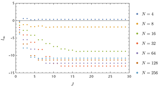
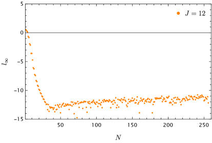
Figure 1: Top: Plot showing the $l_{\infty}$ of the relative error from the exact and numerical solution with number of Chebyshev nodes $N$ versus the number of jumps $J$. It is readily clear that for optimal implementations of the algorithm one needs to study both these numerical algorithm factors. Bottom: From the plot on the top it is clear the optimal number of nodes is $N=32$ Chebyshev nodes with about $J=12$ jumps.

The discontinuous generalisation to the Lagrange interpolation briefly reviewed above, can then be constructed. This was put forward generically in [52] and later improved by [54, 46, 47, 49]. This method uses higher order jumps as input, where here by jump one means exactly that we can take advantage of the fact we know the location of the particle, $x_{p}$, a priori, such that it holds to write the master field variables a combination of jumps in their fields and derivatives. Hence,

$$\Psi^{(m)}(x_{p}^{+})-\Psi^{(m)}(x_{p}^{-})=J_{m}(t),\ \ \ m=0,1,...,\infty$$ (40)

where explicitly, albeit in $(t,r)$ coordinates this have been given for the first $m=\{0,1\}$ orders in Eq.(22, 23) and will be later specified in hyperboloidal coordinates after it has been adequately incorporated within the Lagrangian method described above.

Essentially one takes the weak-form of the solution to the wave-like functions as given in Eq.(7) and rewrite it as a generic collocation polynomial

$$p(x)=p_{+}(x)\Theta(x-x_{p})+p_{-}(x)\Theta(x_{p}-x),$$ (41)

where the right/left interpolating polynomials are given respectively as

$$p_{+}(x)=\sum^{N}_{j=0}c^{+}_{j}(x_{p})^{j},\ \ \ p_{-}(x)=\sum^{N}_{j=0}c^{-}_{j}(x_{p})^{j}.$$ (42)

By solving Eqs. (42) as a system of algebraic equations with the collocation conditions given by,

$$\Psi_{i}=\left\{\begin{array}[]{ccc}p_{+}(x_{i}),&\qquad x_{i}>x_{p},\\ p_{-}(x_{i}),&\qquad x_{i}<x_{p},\end{array}\right.$$ (43)

one determines half of the $(2N+2)$ polynomial coefficients, $c^{\pm}_{j}$. The remaining coefficients are then determined by imposing the jump conditions in Eq. (41) as,

$$p_{+}^{(m)}(x_{p})-p_{-}^{(m)}(x_{p})=\left\{\begin{array}[]{ccc}J_{m},&m=0,1,...,M\\ 0,&m=M+1,...,N\end{array}\right..$$ (44)

where here $M$ ranges from $[-1,...,N]$ and the $M=N+1$ jumps are left unspecified until when studying the number of jumps optimal to the algorithm’s implementation for the particular physical model here studied. Everything in the LBP is then rewritten as, $\pi_{j}(x)$, as given in Eq. (33) which varies depending on whether one chooses to work with spectral Eq. (36) or a finite-difference Eq. (39) collocation methods. It then suffices to solve algebraically the interpolating piecewise polynomial

$$p^{\pm}(x)=\sum^{N}_{j=0}C^{\pm}_{j}(x_{p})\pi_{j}(x).$$ (45)

Specifically one has the algebraic conditions,

$$C^{+}_{j}(x_{p})=\Psi_{j}+\Theta(x_{p}-x_{j})g(x_{j}-x_{p}),$$ (46)

$$C^{-}_{j}(x_{p})=\Psi_{j}-\Theta(x_{j}-x_{p})g(x_{j}-x_{p}),$$ (47)

where,

$$g(x_{j}-x)=\sum^{M}_{m=0}\frac{J_{m}}{m!}(x_{j}-x_{p})^{m}$$ (48)

are the weights computed from the jump conditions derived at the discontinuity $x_{p}$. Finally, substituting Eqs. ((45)-(47)) into Eq. (41) we get the generic interpolating piecewise polynomial,

$$p(x)=\sum^{N}_{j=0}\bigg{[}\Psi_{j}+\Delta_{\Psi}(x_{j}-x_{p};x-x_{p})\bigg{]}\pi_{j}(x)$$ (49)

where the $\Delta_{\Psi}$ function is given by

$$\Delta_{\Psi}(x_{j}-x_{p};x-x_{p})=$$

$$=\bigg{[}\Theta(x-x_{p})\Theta(x_{p}-x_{j})-\Theta(x_{p}-x)\Theta(x_{j}-x_{p})\bigg{]}g(x_{j}-x_{p})\ \ \ \ \ \ \$$

$$=\bigg{[}\Theta(x_{i}-x_{p})-\Theta(x_{j}-x_{p})\bigg{]}g(x_{j}-x_{p}).\ \ \ \ \ \$$ (50)

In the end one approximate our master field variables as given in eq.(7) by

$$\Psi(t,x)\approx\sum^{N}_{j=0}\bigg{[}\Psi_{j}(t)+\Delta_{\Psi}(x_{j}-x_{p}(t);x-x_{p}(t))\bigg{]}\pi_{j}(x).$$ (51)

To be precise, all the differential operators in Eq.(7) and further specified in Eq.(121) and Eqs.(153-157), are discretised as,

$$\partial_{x}^{n}(t,x)\Psi|_{x=x_{i}}=p^{(n)}(x)=\sum^{N}_{j=0}D^{(n)}_{ij}\Psi_{j}+s_{i}^{(n)}(t),\ \ \ \$$ (52)

where $s^{(n)}_{i}(t)$ is given as

$$s^{(n)}_{i}(t)=\sum^{N}_{j=0}D^{(n)}_{ij}\Delta_{\Psi}\big{(}x_{j}-x_{p}(t);x_{i}-x_{p}(t)\big{)}$$ (53)

and the user-specifiable high-order jumps in Eq. (48) obtained through the computation of the higher order recurrence relation given as,

$$J_{m+2}(t)=-\frac{1}{(f^{2}_{p}-\dot{r}^{2}_{p})}\sum^{\infty}_{m=0}\bigg{(}\ddot{J}_{m}(t)$$

$$+\sum^{m}_{k=0}{m\choose k}\bigg{[}-\rho^{(k)}(r_{p})J_{m+1-k}(t)+V^{(k)}(r_{p})J_{m-k}(t)\bigg{]}$$

$$-\sum^{m}_{k=1}{m\choose k}\eta^{(k)}(r_{p})J_{m+2-k}(t)\bigg{)}.$$ (54)

Furthermore the initialising jumps $J_{0}(t),J_{1}(t)$ are generically given as in Eqs.(22, 23) for when the wave equation is for example as given in Eq.(219) for the $\Psi(t,r)$ field. Shortly the recurrence relation for the field in $\Psi(t,x)$ will be specified. In what follows, one will also apply the machinery just explained when solving wave and wave-like equations in an hyperboloidal coordinate chart where $(t\rightarrow t(\tau,\sigma),r\rightarrow r(\sigma))$. One notes this implementation has thoroughly be explained in previous work [49].

3.2.3 Example of discontinuous differentiation of a simple spatial function

To illustrate the usefulness of the above scheme as well as understand the required numerical optimisation factors associated with resolving functions with discontinuities in space, the following discontinuous function

$$f(x)=\sin(\pi|x-x_{p}|)$$ (55)

is considered in the spatial domain $x\in[-1,1]$ and where $x_{p}$ is the discontinuity at say $x_{p}=0.001$. Exact higher order derivatives of this function can be found via,

$$f^{n}_{\textbf{E}}(x)=\left\{\begin{array}[]{ccc}f^{(n)}(x)^{+}&\text{for}&x>x_{p},\\ f^{(n)}(x)^{-}&\text{for}&x<x_{p},\\ \frac{f^{(n)}(x)^{+}-f^{(n)}(x)^{-}}{2}&\text{else},\end{array}\right.$$ (56)

where the subscript E indicates the solution is in exact form. The analytic jumps associated with this function and its derivatives are given by,

$$J_{m}=\frac{1}{m!}\bigg{[}\lim_{x\rightarrow x_{p}^{+}}f^{(m)}(x)-\lim_{x\rightarrow x_{p}^{-}}f^{(m)}(x)\bigg{]},\hskip 25.6073ptm=0,1,2,...,M$$ (57)

where $M$ is the user-specifiable number of jumps.

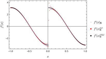
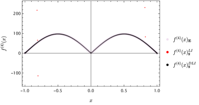
Figure 2: Plots of the exact spatial discontinuous function as given by Eq.(56) against the numerical solution are obtained with traditional Lagrangian smooth interpolation methods and followed with the correction introduced by the discontinuous algorithm. One demonstrates the accuracy of the algorithm by considering both the first- and fourth- order spatial derivatives.

To construct the numerical solution $f^{(n)}_{\texttt{N}}$ one makes use of Eq.(50), now given as,

$$f^{(n)}(x_{i})_{\texttt{N}}\approx p^{(n)}(x_{i})=\sum^{N}_{j=0}D^{(n)}_{ij}[f_{j}+\Delta(x_{j}-x_{p};x_{i}-x_{p})],$$ (58)

and here $N$ highlights this is the numerical solution, $f_{j}=f(x_{j})$ and we now substitute Eq.(50) here to get,

$$f^{(n)}(x_{i})_{\texttt{N}}\approx\sum^{N}_{j=0}D^{(n)}_{ij}[f_{j}+g_{j}\Theta_{i}-g_{j}\Theta_{i}],$$ (59)

where $g_{j}=g(x_{j}-x_{p})$ and $\Theta_{i}=\Theta(x_{i}-x_{p})$. This amounts to simple vector-matrix and matrix-matrix multiplication obtained in Mathematica for example as,

fn = Dn.f + (Dn.g)*h - Dn.(g*h)

where fn $=f(x_{i})_{\texttt{N}}$, f $=f(x_{j})$ Dn $=D^{(n)}_{ij}$, $h=\Theta_{i/j}$ and $g=g_{i/j}$ vectors. It is important to emphasise here that the numerical accuracy associated with discontinuous collocation Lagrange interpolation methods depends on two main factors which are user-specifiable:

1. Number of nodes;

2. Number of jumps;

From the numerical experiments showed in Fig.(1) it’s clear high accuracies are possible for $N=32$ Chebyshev nodes, using Eq.(36), and with $J=12$ nodes. In Fig.(2) one compares the numerical solution, $f^{\prime}(x)^{DLI}$, for the first order derivative against the exact solution $f^{\prime}(x)^{E}$ and the solution that would be obtained if the discontinuous corrections, given by $\Delta$ in Eq.(58), were not to be included [53, 47].

3.3 High order discontinuous time integration

3.3.1 The IMplicit-Turned-EXplicit IMTEX Hermite geometric integrators and relatives - addressing difficulty $(3)$

Figure 3: Fractional energy error from the evolution of Eq.(25) as given in Ref.[49] with no RHS terms i.e $\mathcal{S}=S_{lm}(\tau,\sigma)=0$. One observes both HF EX RK and IMTEX Hermite integrators errors are bounded, with lowest order IMTEX integrators significantly outperforming even the highest HF EX RK schemes. Furthermore, it is observed at this juncture, there is no point in using an Hermite IMTEX scheme of order higher than 4, this is likely due to the build-up of round-off error and the fact most of the residual error comes from the spatial discretisation which becomes more significant as the order of Hermite IMTEX increases.

Even though the above resolves difficulty $(1)$ in the spatial direction, one still needs to address how the discontinuity is resolved in the time direction to fully accuratelly solve for difficulty $(1)$. However, before one does so, the work done in [48, 49] will be revisited and difficulty $(3)$ will be addressed. One’s motivation here is two-fold. Firstly, before distributionally sourced wave equation of the type Eq.(7) are numerically solved, the effect that increasing the order of integration of these numerical schemes has on the numerical accuracy and speed of the numerical solutions must be clearly understood. Secondly, one wishes to highlight the differences between a purely explicit EX non-geometric time integrator such as Runge-Kutta EX RK scheme and the novel IMplicit-Turned-EXplicit, i.e the IMTEX Hermite integration scheme for both homogeneous and distributionally-sourced wave-like equations.

In Sec. 3.2.1 it was shown how the field variable $\textbf{U}(t,x)$ is discretised in space such that Eq. (29), is effectively reduced to first-order form and solved as a system of coupled ordinary differential equations (ODEs) given as,

$$\frac{d\textbf{U}}{dt}=\textbf{L}\ \textbf{U}+\mathcal{S},$$ (60)

where $\textbf{U}(t,x)\rightarrow\textbf{U}(t)$ with $\textbf{U}(t,x_{i}):=\textbf{U}_{i}(t)$. For now, the source term $\mathcal{S}$ is dropped and one considers only the homogeneous problem. As demonstrated in [48], one starts by applying the fundamental theorem of calculus to solve for the field variable U in time in the form

$$\textbf{U}(t_{n+1})=\textbf{U}(t_{n})+\int^{t_{n+1}}_{t_{n}}\textbf{U}(t)\ dt.$$ (61)

Then approximate $\textbf{U}(t)$ by applying a two-point Taylor expansion, (or a 2-point Hermite interpolant) where one constructs an osculating polynomial such that it matches the values of U and its derivatives at the endpoints $t_{n/n+1}$ approximating the integral in (61) [74, 75, 76]. One then gets the generalised Hermite rule to order $l-1$,

$$\int^{t_{n+1}}_{t_{n}}\textbf{U}(t)dt=\sum^{l}_{k=1}c_{lk}\Delta t^{k}\bigg{(}\textbf{U}^{(k-1)}_{n}+(-1)^{(k-1)}\textbf{U}^{(k-1)}_{n+1}\bigg{)}+\textbf{R}_{l},$$ (62)

where $k$ denotes the order of the time-derivative of our function at any $t_{n}$ such that,

$$\textbf{U}^{(k)}_{n}=\frac{d^{k}\textbf{U}(t)}{dt^{k}}\bigg{|}_{t=t_{n}}.$$ (63)

Furthermore, the expansion coefficients $c_{lk}$ are given as,

$$c_{lk}=\frac{l!(2l-k)!}{k!(2l)!(l-k)!},$$ (64)

and the remainder $\textbf{R}_{l}$ as,

$$\textbf{R}_{l}=(-1)^{l}\frac{(l!)^{2}}{(2l+1)!(2l)!}\Delta t^{2l+1}\textbf{f}^{(2l)}(t),\ \ \ \ \ \ t\in[t_{n},t_{n+1}].$$ (65)

Choosing $l=3$ yields the Lotkin’s rule [77] in implicit, (IM) form, namely

$$\int^{t_{n+1}}_{t_{n}}\textbf{U}(t)dt=\frac{\Delta t}{2}(\textbf{U}_{n}+\textbf{U}_{n+1})+$$

$$\frac{\Delta t^{2}}{10}(\dot{\textbf{U}}_{n}-\dot{\textbf{U}}_{n+1})+\frac{\Delta t^{3}}{120}(\ddot{\textbf{U}}_{n}+\ddot{\textbf{U}}_{n+1})+\mathcal{O}(\Delta t^{7}),$$ (66)

This approximates to,

$$\textbf{U}_{n+1}-\textbf{U}_{n}=\frac{\Delta t}{2}\textbf{L}\cdot(\textbf{U}_{n}+\textbf{U}_{n+1})+$$

$$\frac{\Delta t^{2}}{10}\textbf{L}\cdot(\dot{\textbf{U}}_{n}-\dot{\textbf{U}}_{n+1})+\frac{\Delta t^{3}}{120}\textbf{L}\cdot(\ddot{\textbf{U}}_{n}+\ddot{\textbf{U}}_{n+1}).\ \ \ \ \ \ \ \$$ (67)

Now, one transforms the above equation by matrix inversion to its IMplicit-Turned-EXplicit, IMTEX form and solve as,

$$\bigg{[}\textbf{I}-\frac{\Delta t}{2}\textbf{L}+\frac{\Delta t^{2}}{10}\textbf{L}\cdot\textbf{L}-\frac{\Delta t^{3}}{120}\textbf{L}\cdot\textbf{L}\cdot\textbf{L}\bigg{]}\cdot\textbf{U}_{n+1}=$$

$$\bigg{[}\textbf{I}+\frac{\Delta t}{2}\textbf{L}-\frac{\Delta t^{3}}{10}\textbf{L}\cdot\textbf{L}+\frac{\Delta t^{2}}{120}\textbf{L}\cdot\textbf{L}\cdot\textbf{L}\bigg{]}\cdot\textbf{U}_{n},\ \ \$$ (68)

where Eq. (60) is used to further simplify the $nth-$ order time derivatives, for example, $\dot{\textbf{U}}=\textbf{L}\cdot\textbf{U}$. Given the operator L is linear, one can further optimise the expression above by writting its Horner-form HF and solve this as,

$$\textbf{U}_{n+1}=\textbf{U}_{n}$$

$$+(\Delta t\ \textbf{L})\cdot\bigg{(}\textbf{I}+\frac{1}{60}(\Delta t\ \textbf{L})\cdot(\Delta t\ \textbf{L})\bigg{)}\cdot\textbf{HFH6}\cdot\textbf{U}_{n}$$ (69)

where the HF matrix is specifically given as,

$$\textbf{HFH6}=\bigg{(}\textbf{I}-\frac{\Delta t}{2}\textbf{L}\cdot\bigg{(}\textbf{I}-\frac{\Delta t\ \textbf{L}}{5}\cdot\bigg{(}\textbf{I}-\frac{\Delta t}{12}\textbf{L}\bigg{)}\bigg{)}\bigg{)}^{-1}.$$ (70)

One notes in B.1 all IMTEX evolution schemes are given up to $12th$-order. To obtain Runge-Kutta integration schemes one integrates a 1-point Taylor expansion of $\textbf{U}(t)$ about $t_{n}$,

$$\int^{t_{n+1}}_{t_{n}}\textbf{U}(t)dt=\sum^{l}_{m=1}\frac{\Delta t^{m}}{m!}\textbf{U}^{(m-1)}_{n}+\textbf{R}_{l},$$ (71)

where the remainder is given by,

$$\textbf{R}_{l}=\frac{\Delta t^{l+1}}{(l+1)!}\textbf{U}^{(l)}(t),\hskip 8.5359ptt\in[t_{n},t_{n+1}],$$ (72)

and the $m-th$ derivative by,

$$\textbf{U}^{(m)}_{n}=\frac{d^{m}\textbf{U}(t)}{dt^{m}}\bigg{|}_{t=t_{n}}.$$ (73)

To obtain the traditional Runge-Kutta RK scheme, one treats the derivatives in Eq.(73) as constant polynomial coefficients and eliminates them by evaluating the Taylor $\textbf{U}(t)$ at several points. For an order $7th$ RK scheme the above yields the following EX scheme

$$\textbf{U}_{n+1}=\textbf{U}_{n}+(\textbf{HFRK7}-\textbf{I})\cdot\textbf{U}_{n},$$ (74)

where HFRK7 matrix is given as,

$$\textbf{HFRK7}=\textbf{I}+\textbf{A}\cdot\bigg{(}\textbf{I}+\textbf{A}\cdot\bigg{(}\frac{1}{2}\textbf{I}+\textbf{A}\cdot\bigg{(}\frac{1}{6}\textbf{I}+$$

$$\textbf{A}\cdot\bigg{(}\frac{1}{24}\textbf{I}+\textbf{A}\cdot\bigg{(}\frac{1}{120}\textbf{A}+\bigg{(}\frac{1}{720}\textbf{I}+\frac{1}{5040}\textbf{A}\bigg{)}\cdot\textbf{A}\bigg{)}\bigg{)}\bigg{)}\bigg{)}.$$ (75)

One notes EX RK schemes can be found from orders $2th$ to $6th$ in B.2.

Order of HF IMTEX NH	Accuracy, $\eta$	Wall-clock times, s
Order 2, NH2	$2.5\times 10^{-14}$	$5.1072372$
Order 4, NH4	$7.3\times 10^{-15}$	$4.9639754$
Order 6, NH6	$3.8\times 10^{-15}$	$5.2465613$
Order 8, NH8	$3.6\times 10^{-14}$	$5.4844739$
Order 10, NH10	$2.2\times 10^{-14}$	$6.1766433$
Order 12, NH12	$4.0\times 10^{-14}$	$6.1136290$
Order of HF NRK	Accuracy, $\eta$	Wall-clock times, s
Order 2, RK2	$5.7\times 10^{-5}$	$5.3512382$
Order 3, RK3	$1.9\times 10^{-5}$	$5.6920472$
Order 4, RK4	$4.4\times 10^{-9}$	$6.1857173$
Order 5, RK5	$8.6\times 10^{-10}$	$6.0316653$
Order 6, RK6	$1.9\times 10^{-13}$	$6.2187127$
Order 7, RK7	$2.2\times 10^{-14}$	$6.0237433$

Table 2: Comparison between the accuracy and computational wall-clock times of the different explicit EX numerical integration schemes. Firstly, one gives the results for the numerical IMTEX Hermite NH scheme optimised to Horner-Form HF and the optimised Runge-Kutta RK EX. One observes that an order 7 RK EX scheme is required for competitive accuracy with even the lowest order IMTEX Hermite scheme.

Remarkably, it is needed to extend the Runge-Kutta scheme to $7th$ order to achieve the same results as with our lowest order integration scheme, as evidenced by Table 3 and Fig.(3). Furthermore, it’s observed that a plateau seems to be reached at about $10^{-15}$ accuracy for IMTEX Hermite schemes, this is because most of the residual error stems from the spatial discretisation which becomes more significant with increasing order of integration due to the increase in the number of operators which increases round-off error. This can potentially be mitigated with the implementation of error minimisation algorithm such as compensation summation and performing the operations prior to the evolution with higher precision (higher than 16). At this juncture, one has not explored this but it is left as subject for future work. The merits of IMTEX over traditionally EX explicit schemes are obvious, furthermore IMTEX schemes preserve symplectic structure and are energy conserving both exactly and numerically for quadratic Hamiltonian’s. One refers the reader to B.3 for explicit proof of these proprieties. It is with this conservation proprieties in mind that one selects IMTEX as the time-stepper to resolve difficult $(3)$, implementing DiscoTEX. However in the next sections one will also show solutions where the implicit scheme is used, implementing DiscoIMP, this will be compared and discussed. Explicit schemes can also be constructed with the EX RK HF optimised schemes, and one refers the reader to [47] where this has been implemented and compared, via the evolution algorithm DiscoEX.

3.3.2 Discontinuous time integration via Hermite interpolation higher order formulas - resolving difficulty $(1)$ in the time dimension

One now resumes the problem raised by difficulty $(1)$, resolved in the spatial direction in Section 3.2, and addresses how to resolve the presence of a discontinuity in the time-direction. This can be achieved by correcting the time-integration algorithms presented above to the non-smooth case. Here, it is shown how once again one can use the method of undetermined coefficients to accommodate for the discontinuous nature of the problem by writing the integrals as piecewise interpolating polynomials and using the known jump conditions to solve the algebraic system of equations. In this section it is shown how to do this for $6^{th}$ order, this was an important step when deciding on what order of algorithm to use when applying these methods to the self-force problem, such as in [49]. Furthermore, this work is complemented by B.4 where the schemes from $2th$ to $12th$ orders are corrected as one has done in the preceding section with B.1. The description of this procedure was done initially at second-order by [52] and later improved to higher orders by this author and collaborators.

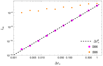
Figure 4: Numerical error associated with the evaluation of the integral in Eq.(91) and with the numerical scheme highlighted in Eq.(66) corrected by incorporating the discontinuous behaviour through the discontinuous time-integration rule given in Eq.(89). For an order-6 integration scheme sixth-order convergence is observed as given by the DH6 line. For a smooth integrator as given by line SH6 inaccurate results are recorded. In B.4.2 one further shows in Fig.(16), the plots for a second- and fourth-order discontinuous time-integrator scheme where second- and fourth-order convergence are observed as expected.

One starts by considering the first order differential equation,

$$\frac{dy}{dt}=f(t,y(t)),$$ (76)

on a small time interval $[t_{\nu},t_{\nu+1}]$. Applying the fundamental theorem of calculus one has,

$$y(t_{\nu+1})-y(t_{\nu})=\int^{t_{\nu}}_{t_{\nu+1}}f(t,y(t))dt.$$ (77)

For the smooth case, as demonstrated in the previous section this amounts to a simple approximant such as that given in Eq.(66). For the non-smooth case one incorporates the discontinuous behaviour by constructing the interpolant as a piecewise polynomial,

$$f(t,y(t))\approx p(t)=p_{+}(t)\Theta(t-t_{\times})+p_{-}(t)\Theta(t_{\times}-t),$$ (78)

where $t_{\times}$ is the point where the function is discontinuous such that $t_{\times}\in[t_{\nu},t_{\nu+1}]$ and $f$ is approximated as $p_{+}$ in $[t_{\times},t_{\nu+1}]$ and $p_{-}$ in $[t_{\nu},t_{\times}]$. Specifically one has

$$p_{+}(t)=a_{0}+a_{1}t+a_{2}t^{2}+a_{3}t^{3}+a_{4}t^{4}+a_{5}t^{5},$$ (79)

$$p_{-}(t)=b_{0}+b_{1}t+b_{2}t^{2}+b_{3}t^{3}+b_{4}t^{4}+b_{5}t^{5}.$$ (80)

One has 12 unknown coefficients, however, as explained before and derived in Section 2, the jump conditions are known so one can impose the following collocation conditions:

$$p_{-}(t_{\nu})=f_{\nu},p_{+}(t_{\nu+1})=f_{\nu+1},$$ (81)

$$p_{-}^{\prime}(t_{\nu})=df_{\nu},\hskip 5.69046ptp_{+}^{\prime}(t_{\nu+1})=df_{\nu+1},$$ (82)

$$p_{-}^{\prime\prime}(t_{\nu})=ddf_{\nu},\hskip 5.69046ptp_{+}^{\prime\prime}(t_{\nu+1})=ddf_{\nu+1},$$ (83)

$$p_{-}^{\prime\prime\prime}(t_{\nu})=dddf_{\nu},\hskip 5.69046ptp_{+}^{\prime\prime\prime}(t_{\nu+1})=dddf_{\nu+1},$$ (84)

$$p_{+}(t_{\times})-p_{-}(t_{\times})=\textbf{J}_{0},$$ (85)

$$p_{+}^{\prime}(t_{\times})-p_{-}^{\prime}(t_{\times})=\textbf{J}_{1},$$ (86)

$$p_{+}^{\prime\prime}(t_{\times})-p_{-}^{\prime\prime}(t_{\times})=\textbf{J}_{2},$$ (87)

$$p_{+}^{\prime\prime\prime}(t_{\times})-p_{-}^{\prime\prime\prime}(t_{\times})=\textbf{J}_{3}.$$ (88)

With these 12 conditions one can now solve for the 12 polynomial coefficients highlighted in Eqs.(79, 80) as a linear system of algebraic equations. The exact $p_{+/-}$ interpolants are given in B.4. Integrating both of the piecewise polynomials yields

$$f(t)_{\texttt{NDH6}}=\frac{\Delta t}{2}\bigg{(}f(t_{\nu})+f(t_{\nu+1})\bigg{)}+$$

$$\frac{\Delta t^{2}}{10}\bigg{(}\dot{f}(t_{\nu})-\dot{f}(t_{\nu+1})\bigg{)}+\frac{\Delta t^{3}}{120}\bigg{(}\ddot{f}(t_{\nu})+\ddot{f}(t_{\nu+1})\bigg{)}+\textbf{J}_{\texttt{H6}}(\Delta t_{\times},\Delta t),\ \ \ \ \ \ \ \$$ (89)

where $\textbf{J}_{\texttt{H6}}(\Delta t_{\times},\Delta t)$ is given by

$$\textbf{J}_{\texttt{H6}}(\Delta t_{\times},\Delta t)=\frac{1}{2}(\Delta t-2\Delta t_{\times})\textbf{J}_{0}+\frac{1}{10}(\Delta t^{2}-5\Delta t\Delta t_{\times}+5\Delta t_{\times}^{2})\textbf{J}_{1}+$$

$$\frac{1}{120}(\Delta t-2\Delta t_{\times})(\Delta t^{2}-10\Delta t\Delta t_{\times}+10\Delta t_{\times}^{2})\textbf{J}_{2}-$$

$$\frac{1}{120}(\Delta t-\Delta t_{\times})\Delta t_{\times}(\Delta t^{2}-5\Delta t\Delta t_{\times}+5\Delta t_{\times}^{2})\textbf{J}_{3}+$$

$$\frac{1}{240}(\Delta t-2\Delta t_{\times})(\Delta t-\Delta t_{\times})^{2}\Delta t_{\times}^{2}\textbf{J}_{4}-$$

$$\frac{1}{720}(\Delta t-\Delta t_{\times})^{3}\Delta t_{\times}^{3}\textbf{J}_{5}.$$ (90)

Similarly to the previous section, the effects of increasing the order of the time-integration of the algorithm has on the accuracy and computational times are thoroughly studied. One refers the reader to B.4.2 where all formulas can be found from order $2^{nd}$ to $12^{th}$. One starts by considering the the time-dependent Legendre polynomial

$$f(t)=P_{5}(t)\Theta(t)+Q_{5}(t)\Theta(t),$$ (91)

where $P_{5}(t),Q_{5}(t)$ are the fifth Legendre polynomials of first and second kind respectively. Introducing a discontinuity at $t_{\times}=0$ in the interval $t\in[-0.55,0.45]$, Eq.(91) admits the following analytical jumps,

$$\textbf{J}_{0}=\frac{8}{15},\ \textbf{J}_{1}=\frac{15}{8},\ \textbf{J}_{2}=-16,\ \textbf{J}_{3}=-\frac{105}{2},$$ (92)

$$\textbf{J}_{4}=384,\ \textbf{J}_{5}=945,\ \textbf{J}_{6}=-3840,\ \textbf{J}_{7}=0,$$ (93)

$$\textbf{J}_{8}=-46080,\ \textbf{J}_{9}=0,\ \textbf{J}_{10}=-1935360,\ \textbf{J}_{11}=0.$$ (94)

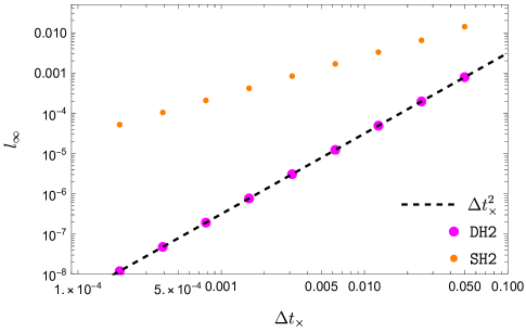
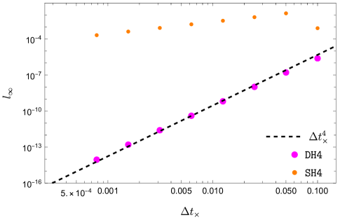
Figure 16: Numerical error associated with the evaluation of the integral in Eq.(91) and with the numerical scheme highlighted in 3.3.1 corrected by incorporating the discontinuous behaviour through the rules given in Eq.(314, 315). As per left plot, for order-2 one observes second-order convergence as given by the DH2 line. For a smooth integrator as given by line SH2 inaccurate results are recorded. Similarly, one shows fourth-order convergence on the right plot as given by the line DH4, whereas without a discontinuous correction the scheme is inaccurate as given by SH4 line.

Integrating analytically the above polynomial in the interval $t\in[-0.55,0.45]$ one gets $\approx 0.1125883303464025$. From Fig.(4) it is observed that the error associated with the discontinuous time-integration rule retrieved in Eq.(89) scales with order 6 as expected. Furthermore the results are complemented with B.4.2 and Fig.(16) showing the discontinuous time integration rule scaling with the expected orders for a second- and fourth-order time-integration method. In all these plots one further includes the result attained if we were to perform a smooth integration as given by Eq.(66) without the discontinuous corrections. To further investigate the effect increasing the order of the integrator had on numerical results the numerical integrals at $\Delta t=0.0001$ are evaluated at the final time $t=0.45$ for all the $12th$ order discontinuous Hermite interpolation schemes. As it is observed in Table 3 increasing after $4th$ order for the same interval the scheme’s accuracy

Order of NDH	Accuracy, $\eta$	Wall-clock times, s
Order 2, NDH2	$3.1396164973385154\times 10^{-9}$	$0.4410348$
Order 4, NDH4	$3.733124920302089\times 10^{-15}$	$3.2397477$
Order 6, NDH6	$3.733124920302089\times 10^{-15}$	$7.083297$
Order 8, NDH8	$3.733124920302089\times 10^{-15}$	$11.21189$
Order 10, NDH10	$3.733124920302089\times 10^{-15}$	$15.4928979$
Order 12, NDH12	$3.733124920302089\times 10^{-15}$	$19.2839227$

Table 3: Here one gives the accuracy and wall-clock computational times of the corrected Hermite integration schemes interpolated to accommodate for time functions which have a discontinuity. One evaluates the function at the same final time of $t_{f}=0.45$ and a time-step of $\Delta t=0.0001$. After 4 orders the same accuracy is attained for this interval while the computational task time significantly increases. These results are further complemented by Figs.(4, 16).

saturates with no improvement, while the computational time significantly increases. These results ultimately motivated our selection of an order-4 scheme when performing the numerics in [49], and the rest of my work in this manuscript and incoming [47]. Furthermore, it is important to note for numerical implementations another optimisation factor emerges:

1. the time $\Delta t$ step-size,

which should be studied before conducting numerical simulations. One also highlights the jumps in the time direction, J are fixed and determined by the order of the discontinuous time-integration algorithm as evidenced by Eq.(89, 90) and the respective equations for the different order integrators given in B.4.2.

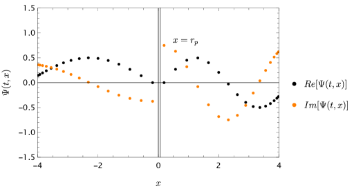
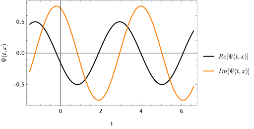
Figure 5: Numerical weak-form solution to $\Psi(t,x)$ obtained via DiscoTEX. Left: Numerical field $\Psi(t,x)$ for a point-particle in time-dependent linear motion $r_{p}(t)=vt$, where $v$ is the particle’s velocity. Specifically, here $r_{p}\approx 0.0634$ at the coordinate-time $t=0.1902$ and $v=1/3$. Right: Waveform for the point-particle computed on the numerical domain $x\in[-4,4]$ and $t\in[-1.521,6.602]$.

3.4 Numerical weak-form solutions to the distributionally sourced wave equation via the DiscoTEX numerical solver

With the technology studied in in Sections 3.2-3.3 one has demonstrated:

• Difficulty $(1)$ - can be accurately resolved in both the space (Section 3.2) and time (Section 3.3) directions through discontinuous collocation methods in both dimensions - Disco;

• Difficulty $(3)$ - can be accurately resolved with suitable Hermite implicit IM, -IMP, or implicit-turned-explicit IMTEX, -TEX, numerical integrators, Section 3.3.1.

• implement solver - DiscoTEX or related solvers such as - DiscoIMP

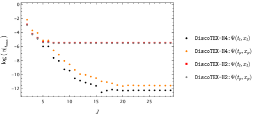
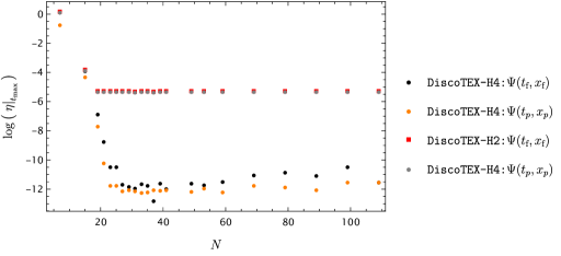
Figure 6: Numerical convergence studies for optimal implementation of DiscoTEX with an order $2$ and $4$ IMTEX Hermite H2/H4 time integrator to meet requirements [REQ 1], [REQ 2] with high accuracy. [REQ 1] is assessed by computing the error of the numerical solution $\Psi(t_{f},x_{f})$ at $\sigma=1$, i.e at infinity $\mathscr{I}^{+}$ against the exact solution as given by Eq.(96). [REQ 2] is assessed by computing the error of the numerical solution $\Psi(t_{p},x_{p})$ via DiscoTEX’s interpolator at the point-particle position $r_{p}(t)=x_{p}$ as given in Eq.(173) against the exact solution evaluate at the same $r_{p}$ particle location. Left: Convergence study determining the optimal number of jumps as $J=20$. Right: Convergence study determining the optimal number of Chebyshev nodes at around $N=34$.

The aim is now to show how one can adapt the numerical method-of-lines recipe framework to incorporate for these corrections which accurately resolve the discontinuous nature of the problem. One will show requirements [REQ 1], [REQ 2] can be accurately met by implementing DiscoTEX: i.e using discontinuous collocation methods to resolve the particle discontinuity in space and time, followed by the use of an IMTEX time-integrator. For the first time, it will be shown how DiscoTEX can be used to complete solutions to equations of Type I as given in Eq.(11, 12), i.e

$$\textrm{Type I:}\ \ \square\Psi(t,x)=F(t)\delta^{\prime}(x-r_{p})+G(t)\delta(x-r_{p}),$$ (95)

$$\Psi(t,x)=-\frac{1}{2}\sin\mathcal{\theta}+\frac{1}{2}{i\mkern 1.0mu}\gamma^{2}[\dot{r}_{p}+\text{sgn}(x-r_{p})]\cos\mathcal{\theta}.$$ (96)

For simplicity, here, defined $F(t)=-{i\mkern 1.0mu}G(t)=-{i\mkern 1.0mu}\cos{t}$. In the body of this work, as explained one will use the method-of-lines framework, hence, to reduce it to a first-order system of equations the master function $\Pi(t,x)=\partial_{t}\Psi(t,x)$ is introduced, with the equation above, now given as

$$\partial_{t}\Psi=\Pi,$$ (97)

$$\partial_{t}\Pi=\partial_{x}^{2}\Psi-F(t)\delta^{\prime}(x-r_{p})-G(t)\delta(x-r_{p}).$$ (98)

As explained in [49, 52] the idea is to use discontinuous collocation methods, as thoroughly explained in Section 3.2.1 through Eqs.(30 - 54), and approximate both master functions as

$$\Psi(t,x)\approx\sum^{N}_{j=0}\bigg{[}\Psi_{j}+\Delta_{\Psi}(x_{j}-r_{p}(t);x-r_{p}t)\bigg{]}\pi_{j}(x),$$ (99)

$$\Pi(t,x)\approx\sum^{N}_{j=0}\bigg{[}\Pi_{j}+\Delta_{\Pi}(x_{j}-r_{p}(t);x-r_{p}t)\bigg{]}\pi_{j}(x),$$ (100)

and the differential operators as,

$$\partial_{(x)}^{n}(t,x)\Psi|_{x=x_{i}}=p^{(n)}(x)$$ (101)

$$=\sum^{N}_{j=0}D^{(n)}_{ij}\Psi_{j}+s_{i}^{(n)}(t),\ \ \ \$$ (102)

with $s^{(n)}_{i}(t)$ given as,

$$s^{(n)}_{i}(t)=\sum^{N}_{j=0}D^{(n)}_{ij}\Delta_{\Psi}\big{(}x_{j}-r_{p}(t);x_{i}-r_{p}(t)\big{)},$$ (103)

where the user-specifiable higher order jumps are given by a recurrence relation of the type given in Eq.(54). This equation, as explained in A, is derived for the case where the wave equation operator is in $(t,r)$ coordinates. Here, one works, as explained, with the version transformed to $(t,x)$ coordinates through a tortoise coordinate transformation as defined in Eq.(7). The methodology explained in A and originally given in [49], in $(t,x)$ greatly simplifies, to,

$$J_{0}(t)=\gamma^{2}(t)F(t),$$ (104)

$$J_{1}(t)=\gamma^{2}(t)\big{[}G(t)-2\dot{J}_{0}(t)-\ddot{r}_{p}(t)J_{0}(t)\big{]},$$ (105)

$$J_{m+2}(t)=\gamma^{2}(t)\big{[}\ddot{J}_{m}(t)-2\dot{r}_{p}\dot{J}_{m+1}(t)-\ddot{r}_{p}(t)J_{m+1}(t)\big{]},$$ (106)

where,

$$\gamma^{2}(t)=\frac{1}{(1-\dot{r}_{p}^{2})}.$$ (107)

This equation was first included in the second version of [52]. Despite multiple efforts by multiple people throughout several years, [52, 80, 81, 82] this equation will only now be fully demonstrated and proven here thanks to the existence of the exact equation as given in Eq.(96) originally derived by Field [28, 68] over a decade ago. As highlighted in Sections 3.1, 3.3 in Eq.s(29, 60) one starts by reducing the problem to a first-order system of differential equations, i.e,

$$\frac{d\textbf{U}}{dt}=\textbf{L}\cdot\textbf{U}+\mathcal{S}+\Upsilon,\ \ \ \textbf{U}=\begin{pmatrix}\Psi(t)\\ \Pi(t)\end{pmatrix},$$

$$\mathcal{S}=\begin{pmatrix}0\\ \textbf{s}_{\Psi}(t)+\textbf{s}_{\Pi}(t)\end{pmatrix},\ \ \Upsilon=\begin{pmatrix}\Upsilon_{\Psi}(t)\\ \Upsilon_{\Pi}(t)\end{pmatrix},\$$ (108)

where all functions were written with respect to time. The matrix evolution operator associated with Eq.(96) is,

$$\textbf{L}=\begin{pmatrix}0&I\\ \textbf{L}_{1}&\textbf{L}_{2}\end{pmatrix}=\hskip 5.69046pt\begin{pmatrix}0&I\\ \textbf{-}\partial_{x}^{2}&0\end{pmatrix}.$$ (109)

For convenience one defines,

$$\begin{pmatrix}\Upsilon_{\Psi}(t)=-[[\Psi]]_{i}\Xi_{i}=-J_{0}(t)*\Xi_{i}\\ \Upsilon_{\Pi}(t)=-[[\Pi]]_{i}\Xi_{i}=-\mathbb{J}_{0}(t)*\Xi_{i}\end{pmatrix}$$ (110)

with $J_{0}(t)$ is as defined in Eq.(104). $\mathbb{J}_{0}(t)$ is the jump associated with the time derivative of the master $\Psi(t,x)$ i.e $\Pi(t,x)$, this can be generically derived as

$$\mathbb{J}(t)=\mathbb{J}_{m}(t)=\partial_{t}(J_{m}(t))-\dot{r}_{p}(t)J_{m+1}(t),$$ (111)

$$\mathbb{J}(t)|_{m=0}=\mathbb{J}_{0}(t)=\partial_{t}(J_{0}(t))-\dot{r}_{p}(t)J_{1}(t).$$ (112)

One refers the reader to A Eq.(254) for a clarification on the derivation of this relation. $[[\Psi]]_{i}$ is as defined in Eq.(19), and $[[\Pi]]_{i}$ is given by

$$[[\Pi]]_{i}=\Pi^{+}(t,r_{p}(t))-\Pi^{-}(t,r_{p}(t)),\hskip 5.69046ptt\rightarrow\frac{x_{i}}{v}$$ (113)

$$\Xi_{i}=\Theta(t_{n+1}-t_{i})\Theta(t_{i}-t_{n}),$$ (114)

where $\Theta$ is as defined in Eq.(18) and $\Xi_{i}$ acts as a switch which turns on these corrections in the time direction for both the $\Psi(t)$ and $\Pi(t)$ master functions when the particle worldline $r_{p}(t)$ crosses the $i-$th grid-point as they are integrated through DiscoTEX at a time $t_{i}\in[t_{n},t_{n+1}]:r_{p}(t)=x_{i}$. One emphasises here a minus sign has been introduced to highlight the correction needed when considering the jumps in the time-direction, this is crucial for algorithm to work. In [52] eq.(C5), even though not necessarily wrong as there are no derivatives of the Dirac distribution as per their eq.(47), the term $\Upsilon_{\Psi}(t)$ it’s just zero as $J_{0}(t)=0$, and hence only Eq.(112).

As in Eq.(109) L only has a differential operator $-\partial_{x}^{2}$ and the source $\mathcal{S}$ simplifies to

$$\mathcal{S}=\begin{pmatrix}0\\ \textbf{s}_{\Psi}(t)+\textbf{s}_{\Pi}(t)=0\end{pmatrix},$$ (115)

$$\mathcal{S}=\begin{pmatrix}0\\ \textbf{s}_{\Psi}(t)\end{pmatrix},$$ (116)

where $\textbf{s}_{\Psi}(t)$ is simply given by

$$\textbf{s}_{\Psi}(t)=\tilde{\textbf{s}}^{(2)}_{\Psi}(t),$$ (117)

$$\tilde{\textbf{s}}^{(2)}_{\Psi}(t)=\sum^{N}_{j=0}D^{(2)}_{ij}\big{[}\Delta_{\Psi}(x_{j}-r_{p};x_{i}-r_{p})\big{]}.$$ (118)

3.4.1 Numerical weak-form solution via DiscoTEX with moving radiation boundary conditions

In this work one will consider and compare both implementations of DiscoTEX with moving radiation boundary conditions [53] and with hyperboloidal slicing [53] recently used in [49]. As demonstrated in [28, 52], one can impose purely outgoing solutions at the first $x_{i=0}$ and last $x_{i=N}$ grid-points, as, respectively

$$\Pi(t,x=a)=\partial_{x}\Psi(x=a),$$ (119)

$$\Pi(t,x=b)=-\partial_{x}\Psi(x=b).$$ (120)

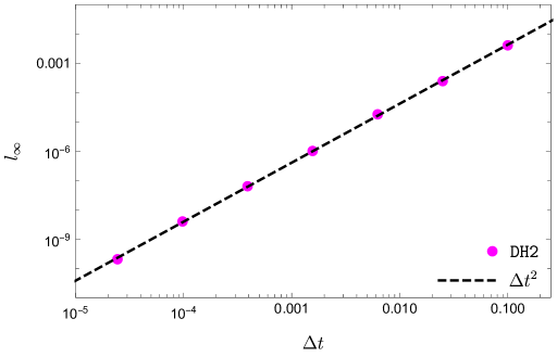
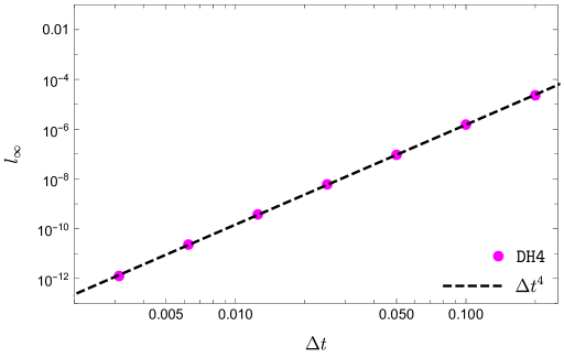
Figure 7: Numerical error associated with computation of the numerical weak-form solution $\Psi(t,x_{f})$ against the exact solution in Eq.(96) with both the discontinuous Hermite integrator of order-2 and order-4, respectively DH2,DH4. Left: For an order-2 integration scheme second-order convergence is observed as given by the DH2 line. Right: For an order-4 integration scheme fourth-order convergence is observed as given by the DH4 line.

Specifically, the wave operator now corrects to

$$\textbf{L}=\begin{pmatrix}0&I\\ \textbf{L}_{1}&\textbf{L}_{2}\end{pmatrix}=\hskip 5.69046pt\begin{pmatrix}0&I\\ \textbf{-}\partial_{x}^{2}&M_{ij}\end{pmatrix},$$ (121)

where $M_{ij}$ is as defined exactly as in their Eq.(B9) and the source term $\mathcal{S}$ is now defined as in Eq.(B9) of [52] and eq.(117) now corrects to,

$$\mathcal{S}=\begin{pmatrix}0\\ \textbf{s}_{\Psi}(t)+\textbf{s}_{\Pi}(t)\neq 0\end{pmatrix}=\begin{pmatrix}0\\ \textbf{s}_{\Psi}(t)+\textbf{s}_{\Pi}(t)\end{pmatrix},$$ (122)

with $\textbf{s}_{\Psi}(t)$ and $\textbf{s}_{\Pi}(t)$ being, respectively defined as,

$$\textbf{s}_{\Psi}(t)=\bar{\textbf{s}}^{(1)}_{\Psi}(t)+\bar{\textbf{s}}^{(2)}_{\Psi}(t)+\bar{\textbf{s}}^{(2)}_{\Psi}(t),$$ (123)

$$\bar{\textbf{s}}^{(2)}_{\Psi}(t)=\sum^{N}_{j=0}\bar{D}^{(2)}_{ij}\big{[}\Delta_{\Psi}(x_{j}-r_{p};x_{i}-r_{p})\big{]},$$ (124)

$$\bar{\textbf{st}}^{(2)}_{\Psi}(t)=\sum^{N}_{j=0}\bar{D}^{(2)}_{ij}\big{[}\partial_{t}\Delta_{\Psi}(x_{j}-r_{p};x_{i}-r_{p})\big{]},$$ (125)

$$\bar{\textbf{s}}^{(1)}_{\Psi}(t)=\sum^{N}_{j=0}\bar{D}^{(1)}_{ij}\big{[}\Delta_{\Psi}(x_{j}-r_{p};x_{i}-r_{p})\big{]},$$ (126)

$$\textbf{s}_{\Pi}(t)=\bar{\textbf{s}}^{(1)}_{\Pi}(t),$$ (127)

$$\bar{\textbf{s}}^{(1)}_{\Pi}(t)=\sum^{N}_{j=0}\bar{D}^{(1)}_{ij}\big{[}\Delta_{\Pi}(x_{j}-r_{p};x_{i}-r_{p})\big{]},$$ (128)

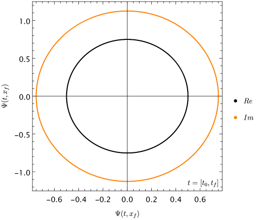
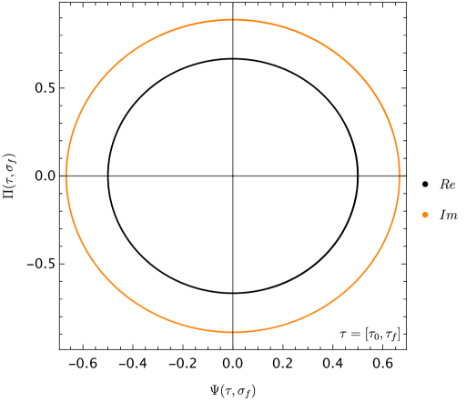
Figure 8: Phase portraits for the numerical weak-form solutions obtained via DiscoTEX with an order $4$ IMTEX Hermite H4 time integrator in both the $(t,r)$ and $(\tau,\sigma)$ coordinate charts. Left: Phase portrait of the numerical weak-form solutions to the field $\Psi(t,x_{f})$, $\Pi(t,x_{f})$ evaluated in the numerical time interval $t\in[-1.521,6.602]$ at the last grid point. Right: Phase portrait of the numerical weak-form solutions to the field $\Psi(\tau,\sigma_{f})$, $\Pi(\tau,\sigma_{f})$ evaluated in the numerical time interval $\tau\in[-1.52,4.50]$ at the last grid point. It is note-worthy to point out that unlike in [49], Fig.(2), here one uses the exact solutions as initial data, whereas in our previous work, we used trivial initial data.

where the bar notation denotes the corrections to the differential operators introduced by the moving radiation boundary conditions framework as defined in [52], more so the term $\bar{\textbf{s}}^{(2)}_{\Psi}(t)$ in Eq.(123) is as given in Eq.(168), and Eq.(130) is its time derivative necessary for an order-4 IMTEX integrator. One also emphasises these equations alternatively re-define $\bar{s}_{i}(t)$ given in the last equation after eq.(B9) of [52]. Furthermore, in this work the results are given through the implementation of an order 4 integration scheme as defined in Eqs.(268, 269), hence one needs to correct their Eq.(B9) [52], given for the implementation of an order 2 implicit scheme, to accommodate for the time-derivative of $s_{i}(t)$ natural arising in an Hermite-order $4th$ integration scheme, following their notation this is explicitly given as

$$\dot{\textbf{s}}_{i}(t)=\dot{s}^{(2)}(t)+D^{(2)}_{i0}\bigg{(}A_{0}\dot{s}^{(1)}_{0}(t)+B_{0}\dot{s}^{(1)}_{N}(t)+C_{0}\dot{s}^{(2)}_{0}(t)+E_{0}\dot{s}^{(2)}_{N}(t)$$

$$-C_{0}\dot{r}^{(1)}_{0}(t)+E_{0}\dot{r}^{(1)}_{N}(t)\bigg{)}+D^{(2)}_{iN}\bigg{(}A_{N}\dot{s}^{(1)}_{0}(t)+B_{N}\dot{s}^{(1)}_{N}(t)+C_{N}\dot{s}^{(2)}_{0}(t)$$

$$+E_{N}\dot{s}^{(2)}_{N}(t)-C_{N}\dot{r}^{(1)}_{0}(t)+E_{N}\dot{r}^{(1)}_{N}(t)\bigg{)},$$ (129)

with, similarly replacing their $\dot{s}^{(1,2)}(t)$ and $\dot{r}^{(1)}(t)$ terms, by

$$\bar{\textbf{st}}^{(2)}_{\Psi}(t)=\sum^{N}_{j=0}\bar{D}^{(2)}_{ij}\big{[}\partial_{t}\Delta_{\Psi}(x_{j}-r_{p};x_{i}-r_{p})\big{]},$$ (130)

$$\bar{\textbf{st}}^{(1)}_{\Psi}(t)=\sum^{N}_{j=0}\bar{D}^{(1)}_{ij}\big{[}\partial_{t}\Delta_{\Psi}(x_{j}-r_{p};x_{i}-r_{p})\big{]},$$ (131)

$$\bar{\textbf{st}}^{(1)}_{\Pi}(t)=\sum^{N}_{j=0}\bar{D}^{(1)}_{ij}\big{[}\partial_{t}\Delta_{\Pi}(x_{j}-r_{p};x_{i}-r_{p})\big{]}.$$ (132)

Furthermore here one highlights that terms in Eqs.(124, 126, 128, 130, 131, 132) are only evaluated at the end points as they emerge from corrections to the radiation boundary conditions as given after Eq.(B9) in [52]. Finally, combining the discontinuous collocation machinery through the spatial corrections described above and correcting the time-integration Hermite IMTEX order-4 scheme eq.(268, 269) with the discontinuous collocation correction in time given by Eq.(315, 320), one has the final evolution scheme, DiscoTEX, namely,

$$\textbf{U}_{n+1}=\textbf{U}_{n}+\textbf{HFH4}\cdot\bigg{[}\textbf{A}\cdot\bigg{[}\textbf{U}_{n}+\frac{\Delta t}{12}\bigg{(}\textbf{s}_{n}+\textbf{s}_{n+1}\bigg{)}\bigg{]}$$

$$+\frac{\Delta t}{2}\bigg{(}\textbf{s}_{n}+\textbf{s}_{n+1}\bigg{)}+\frac{\Delta t^{2}}{12}\bigg{(}\textbf{st}_{n}-\textbf{st}_{n+1}\bigg{)}$$

$$+\Upsilon(t)+\textbf{J}_{\texttt{H4}}(\Delta t_{\times},\Delta t)\Xi\bigg{]},$$ (133)

in the $(t,x)$ coordinate chart. It is left to define the jumps in $\textbf{J}_{\texttt{H4}}(\Delta t_{\times},\Delta t)$. As described in Section 3.3.2, complemented by B.4.2, a fourth-order discontinuous time-integration rule, described by eqs.(315, 320) scheme will impose four jump conditions associated with the jumps of the field equation in the time direction, i.e the time jumps. From eq.(97) it is clear there will be a time jump associated with the integration of $\Pi(t,x)$, and from eq.(98) another due to the integration of $\partial_{x}^{2}\Psi$.

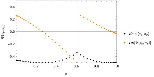
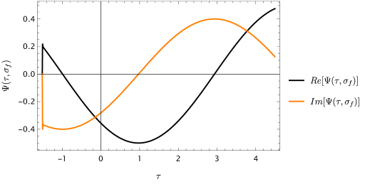
Figure 9: Numerical weak-form solution to $\Psi(\tau,\sigma)$ obtained via DiscoTEX. Left: Numerical field $\Psi(\tau,\sigma)$ for a point-particle in time-dependent linear motion $\xi_{p}(\tau_{c})$, where $v$ is the particle’s velocity. Specifically, here $\xi_{p}\approx 0.608$ at the coordinate-time $\tau_{c}\approx 0.876$ and $v=1/4$. Right: Waveform for the point-particle computed on the numerical domain $\sigma\in[0,1]$ and $\tau\in[-1.52,4.50]$.

This prompts the effective vector,

$$\textbf{J}_{j}(t)=\begin{pmatrix}\mathbb{JJ}_{j}(t)\\ \mathcal{JJ}_{j}(t)\end{pmatrix}=\begin{pmatrix}{\mathbb{J}_{0}(t),\mathbb{K}_{0}(t),\mathbb{L}_{0}(t),\mathbb{M}_{0}(t)}\\ {\mathcal{J}_{0}(t),\mathcal{K}_{0}(t),\mathcal{L}_{0}(t),\mathcal{M}_{0}(t)}\end{pmatrix},$$ (134)

where here $j=0,..3,$ and it depends on the order of the integration scheme used. As explained just before Section 3.3 ends and Section 3.4 starts, one uses an order-4 scheme so only 4 jumps will be necessary. Concretely $\mathbb{J}_{0}$ is as given in Eq.(111, 112), the other jumps are given as,

$$\mathbb{K}_{m}(t)=\partial_{t}(\mathbb{J}_{m}(t))-\dot{r}_{p}(t)\mathbb{J}_{m+1}(t),$$ (135)

$$\mathbb{K}(t)|_{m=0}=\mathbb{K}_{0}(t)=\partial_{t}(\mathbb{J}_{0}(t))-\dot{r}_{p}(t)\mathbb{J}_{1}(t)=\mathbb{JJ}_{1},$$ (136)

$$\mathbb{L}(t)=\partial_{t}(\mathbb{K}_{m}(t))-\dot{r}_{p}(t)\mathbb{K}_{m+1}(t),$$ (137)

$$\mathbb{L}_{0}(t)|_{m=0}=\mathbb{L}_{0}(t)=\partial_{t}(\mathbb{K}_{0}(t))-\dot{r}_{p}(t)\mathbb{K}_{1}(t)=\mathbb{JJ}_{2},$$ (138)

$$\mathbb{M}_{m}(t)=\partial_{t}(\mathbb{L}_{m}(t))-\dot{r}_{p}(t)\mathbb{L}_{m+1}(t),$$ (139)

$$\mathbb{M}_{0}(t)|_{m=0}=\mathbb{M}_{0}(t)=\partial_{t}(\mathbb{L}_{0}(t))-\dot{r}_{p}(t)\mathbb{L}_{1}(t)=\mathbb{JJ}_{3},$$ (140)

and $\mathcal{JJ}_{j=1,2,3}$ are given as,

$$\mathcal{K}_{0}(t)=\partial_{t}(\mathcal{J}_{m}(t))-\dot{r}_{p}(t)\mathcal{J}_{m+1}(t),$$ (141)

$$\mathcal{K}(t)|_{m=0}=\mathcal{K}_{0}(t)=\partial_{t}(\mathcal{J}_{0}(t))-\dot{r}_{p}(t)\mathcal{J}_{1}(t)=\mathcal{JJ}_{1},$$ (142)

$$\mathcal{L}(t)=\partial_{t}(\mathcal{K}_{m}(t))-\dot{r}_{p}(t)\mathcal{K}_{m+1}(t),$$ (143)

$$\mathcal{L}_{0}(t)|_{m=0}=\mathcal{L}_{0}(t)=\partial_{t}(\mathcal{K}_{0}(t))-\dot{r}_{p}(t)\mathcal{K}_{1}(t)=\mathcal{JJ}_{2},$$ (144)

$$\mathcal{M}_{m}(t)=\partial_{t}(\mathcal{L}_{m}(t))-\dot{r}_{p}(t)\mathcal{L}_{m+1}(t),$$ (145)

$$\mathcal{M}_{0}(t)|_{m=0}=\mathcal{M}_{0}(t)=\partial_{t}(\mathcal{L}_{0}(t))-\dot{r}_{p}(t)\mathcal{L}_{1}(t)=\mathcal{JJ}_{3}.$$ (146)

Finally the vectors $\textbf{J}_{0}(t),\textbf{J}_{1}(t),\textbf{J}_{2}(t),\textbf{J}_{3}(t)$ define the necessary time jumps for successful implementation of the discontinuous time-integration rule described by $\textbf{J}_{\texttt{H4}}(\Delta t_{\times},\Delta t)$ in eqs.(315, 320) and eqs.(C8-C32) of [49] (in that work $\textbf{J}_{\texttt{H4}}(\Delta t_{\times},\Delta t)$ = 0, as explained, as we modelled a circular orbit). Additionally, one explicitly gives the first few jumps in both the spatial and time direction through C.1-C.2. An alternative evolution algorithm is given in C.6 using the purely implicit IM Hermite time-integration scheme, hereafter named DiscoIMP. Shortly these implementations will be discussed, after the following section. Before the numerical calibrations necessary for optimal implementation of DiscoTEX, and DiscoIMP, the problem will be considered in a new coordinate chart as an attempt at resolving difficulty $(2)$.

3.4.2 Numerical weak-form solution via DiscoTEX with hyperboloidal slicing as an alternative to incorporation of boundary conditions

The development of DiscoTEX was mostly motivated with application to numerical black hole perturbation theory in mind and hence one of the main goals is the ability to accurately extract information at both the black hole horizon and infinity. As explained in [49], deciding on what boundary conditions to implement has lead to what is known as the outer radiation boundary problem, where it is not entirely clear if the extrapolated information at these boundaries will be contaminated from the implementation of boundary conditions such as those described above. In the past decade, the gravitational self-force numerical relativity community has decided to use hyperboloidal methods to resolve this problem motivated by the work of [83]. There have been numerous implementations of these slices, though here one highlights the works of [84, 85] as they had previously attempted these problem by implementation of boundary conditions described above with the same numerical strategies to resolve difficulties $1)$ and $3)$, also see Table 8. The core idea of hyperboloidal slicing is to parameterise the spacetime with a compact radial coordinate defined on an hyperboloidal time surface, essentially the coordinate map $(t\rightarrow t(\tau,\sigma),x\rightarrow x(\sigma))$ [62] is applied. The technique here used to construct these slices is the “scri-fixing technique” [61]. The coordinate chart is mapped as

$$t=\tau-H(\sigma),\hskip 5.69046ptx=\frac{1}{2}\bigg{(}\frac{1}{\sigma}+\ln{(1-\sigma)}-\ln{\sigma}\bigg{)}.$$ (147)

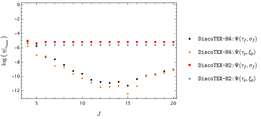
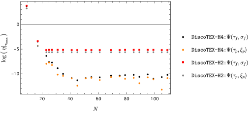
Figure 10: Numerical convergence studies for optimal implementation of DiscoTEX with an order $2$ and $4$ IMTEX Hermite H2/H4 time integrator to meet requirements [REQ 1], [REQ 2] with high accuracy. [REQ 1] is assessed by computing the error of the numerical solution $\Psi(\tau_{f},\sigma_{f})$ at $\sigma=1$, i.e at infinity $\mathscr{I}^{+}$ against the exact solution as given by Eq.(149). [REQ 2] is assessed by computing the error of the numerical solution $\Psi(\tau_{p},\xi_{p})$ via DiscoTEX’s interpolator at the point-particle position $\xi_{p}(\tau_{c})=\xi_{p}$ as given in Eq.(170) against the exact solution evaluate at the same $\xi_{p}$ particle location. Left: Convergence study determining the optimal number of jumps as $J=15$. Right: Convergence study determining the optimal number of Chebyshev nodes at around $N=45$.

It is important to highlight that whereas the map of the time coordinate is exactly the same as we described in [49], here the tortoise coordinate $x$ is directly mapped and not $r$. The height function $H(\sigma)$ is given by,

$$H(\sigma)=\frac{1}{2}\bigg{[}\ln{(1-\sigma)}-\frac{1}{\sigma}+\ln{\sigma}\bigg{]}$$ (148)

as originally introduced by [63, 64, 65, 66]. As in Eq.(96), one now has the following exact equation of Type I,

$$\textrm{Type I:}\ \ \square\Psi[\tau,\sigma]=F(\tau)\delta^{\prime}(\sigma-\xi_{p})+G(\tau)\delta(\sigma-\xi_{p}).$$ (149)

The master function and related functions transform from $\Psi(t,x)\rightarrow\Psi(t(\tau,\sigma),x(\sigma))$, which here are loosely simply denoted by $\Psi(\tau,\sigma)$, the final wave equation can be retrieved by applying the following equation as given originally in [64],

$$\bigg{[}\bigg{(}1-\bigg{(}\frac{H^{\prime}}{x^{\prime}}\bigg{)}\bigg{)}\partial_{\tau}^{2}-\frac{2}{x^{\prime}}\bigg{(}\frac{H^{\prime}}{x^{\prime}}\bigg{)}\partial_{\tau}\partial_{\sigma}-\frac{1}{x^{\prime}}\bigg{(}\frac{H^{\prime}}{x^{\prime}}\bigg{)}^{\prime}\partial_{\tau}-\frac{1}{x^{\prime}}\partial_{\sigma}\bigg{(}\frac{1}{x^{\prime}}\partial_{\sigma}\bigg{)}\bigg{]}\Psi(\tau,\sigma)=0,$$ (150)

where prime indicates derivative with respect to $\sigma$. The equation now reads,

$$\square\Psi(\tau,\sigma)=\mathcal{S}(\tau,\sigma),$$ (151)

with,

$$\square\Psi=\bigg{(}-\Gamma(\sigma)\partial^{2}_{\tau}+\varepsilon(\sigma)\partial_{\sigma}\partial_{\tau}+\varrho(\sigma)\partial_{\tau}+\chi(\sigma)\partial^{2}_{\tau}+\iota(\sigma)\partial_{\sigma}\bigg{)}\Psi.$$ (152)

The coefficients above read,

$$\Gamma(\sigma)=-4\sigma^{2}(-1+\sigma^{2}),$$ (153)

$$\varepsilon(\sigma)=-4(-1+\sigma)\sigma^{2}(-1+2\sigma^{2}),$$ (154)

$$\varrho(\sigma)=-8(-1+\sigma)\sigma^{3},$$ (155)

$$\chi(\sigma)=-4(-1+\sigma)^{2}\sigma^{4},$$ (156)

$$\iota(\sigma)=-4(-1+\sigma)\sigma^{3}(-2+3\sigma),$$ (157)

where, as in [49], one emphasises that the function $\chi(\sigma)$ vanishes at the boundaries where $\sigma=\{0,1\}$, reflecting the outflow behaviour automatically enforced by this hyperboloidal slicing at the future null infinity and the horizon and thus naturally imposes boundary conditions at $\sigma=0$ and $\sigma=1$. The term $\mathcal{S(\tau)}$ is place-hold notation to denote the distributionally source function as only a time-dependent function as before. One will shortly explain how this is handled. The first order reduction of the PDE into a couple of differential equations goes as explained in Eq.(122) in the new coordinate chart, but now the operator L is described by the operators,

$$\textbf{L}_{1}=\frac{1}{\Gamma(\sigma)}\bigg{(}\chi(\sigma)\partial^{2}_{\sigma}+\iota(\sigma)\partial_{\sigma}\bigg{)},$$ (158)

$$\textbf{L}_{2}=\frac{1}{\Gamma(\sigma)}\bigg{(}\varepsilon(\sigma)\partial_{\sigma}-\varrho(\sigma)\bigg{)},$$ (159)

where, for convenience as described in [49], the tilde notation is introduced to denote division of the coefficients in the operators by $\Gamma(\sigma)$, e.g, $\tilde{\varepsilon}(\sigma)=\varepsilon(\sigma)/\Gamma(\sigma)$. One also emphasises the wave-equation here is different from the equation described in [49]. Here, one studies just the flat spacetime and not the Schwarzschild spacetime. The term $\Upsilon$ is defined as Eq.(110) but now with respect to the $\tau$ quantity. One simply has,

$$\begin{pmatrix}\Upsilon_{\Psi}(\tau)=[[\Psi]]_{i}\Xi_{i}=J_{0}(\tau)*\Xi_{i}\\ \Upsilon_{\Pi}(\tau)=[[\Pi]]_{i}\Xi_{i}=\mathbb{J}_{0}(\tau)*\Xi_{i}\end{pmatrix}.$$ (160)

The reader is directed to C.3, where it is explained how $J_{0}(\tau),J_{1}(\tau)$ are obtained in the new chart by the correct application of the Dirac delta-distribution proprieties. For clarity, the time jumps are similarly defined as,

$$\mathbb{J}(\tau)=\mathbb{J}_{m}(\tau)=\partial_{t}(J_{m}(\tau))-\dot{\xi}_{p}(\tau)J_{m+1}(\tau),$$ (161)

$$\mathbb{J}(\tau)|_{m=0}=\mathbb{J}_{0}(\tau)=\partial_{t}(J_{0}(\tau))-\dot{\xi}_{p}(\tau)J_{1}(\tau),$$ (162)

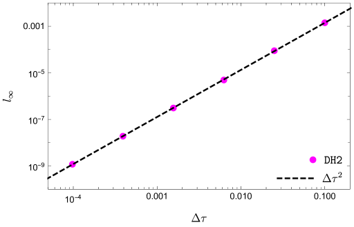
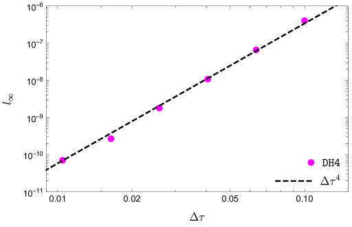
Figure 11: Numerical error associated with computation of the numerical weak-form solution $\Psi(\tau,\sigma_{f})$ against the exact solution in Eq.(149) with both the discontinuous Hermite integrator of order-2 and order-4, respectively DH2,DH4. Left: For an order-2 integration scheme second-order convergence is observed as given by the DH2 line. Right: For an order-4 integration scheme fourth-order convergence is observed as given by the DH4 line.

where $\xi_{p}(\tau)$ denotes the new particle location in the hyperboloidal coordinate chart. The vector $\mathcal{S}$ is now described by,

$$\tilde{\textbf{s}}(\tau)=\begin{pmatrix}0\\ \tilde{s}_{\Psi}^{(1)}+\tilde{s}_{\Psi}^{(2)}+\tilde{s}_{\Pi}^{(1)}\end{pmatrix},$$ (163)

as described in [49]. In this work, however, as emphasised through Eqs.(147 - 159) please note the operators are different, even though one uses the same notation. Despite the different governing wave-like equation, here describing Minkowski’s spacetime, the implementation of the discontinuous collocation machinery is similar due to the differential operators describing the evolution operator $\textbf{L}_{1},\textbf{L}_{2}$ being the same i.e one has in $\textbf{L}_{1}$, two spatial first and second order differential operators, and in $\textbf{L}_{2}$ one has one first-order spatial operators. For completion one includes here these operators, originally given in [53, 49]. The differential operators corrected with the discontinuous collocation algorithm are given by,

$$\tilde{\upchi}(\sigma)\partial_{\sigma}^{2}\Psi\bigg{|}_{\sigma=\sigma_{i}}$$

$$=\sum^{N}_{j=0}\bigg{(}\text{diag}(\tilde{\upchi}(\sigma_{i}))\cdot D^{(2)}\bigg{)}_{ij}\big{[}\Psi_{j}+\Delta_{\Psi}(\sigma_{j}-\sigma_{p};\sigma_{i}-\sigma_{p})\big{]},$$

$$\tilde{\iota}(\sigma)\partial_{\sigma}\Psi\bigg{|}_{\sigma=\sigma_{i}}=$$

$$\sum^{N}_{j=0}\bigg{(}\text{diag}(\tilde{\iota}(\sigma_{i}))\cdot D^{(1)}\bigg{)}_{ij}\big{[}\Psi_{j}+\Delta_{\Psi}(\sigma_{j}-\sigma_{p};\sigma_{i}-\sigma_{p})\big{]},$$

$$\tilde{\upvarepsilon}(\sigma)\partial_{\sigma}\Pi\bigg{|}_{\sigma=\sigma_{i}}=$$

$$\sum^{N}_{j=0}\bigg{(}\text{diag}(\tilde{\upvarepsilon}(\sigma_{i}))\cdot D^{(1)}\bigg{)}_{ij}\big{[}\Pi_{j}+\Delta_{\Pi}(\sigma_{j}-\sigma_{p};\sigma_{i}-\sigma_{p})\big{]}.$$

The explicit form of $\tilde{\textbf{s}}(\tau)$ in Eq. (163) containing all the necessary corrections to the differential operators is

$$\tilde{s}_{\Psi}^{(1)}=\sum^{N}_{j=0}\bigg{(}\text{diag}(\tilde{\iota}(\sigma_{i}))\cdot D^{(1)}\bigg{)}_{ij}\big{[}\Delta_{\Psi}(\sigma_{j}-\sigma_{p};\sigma_{i}-\sigma_{p})\big{]},\ \ \$$ (167)

$$\tilde{s}_{\Psi}^{(2)}=\sum^{N}_{j=0}\bigg{(}\text{diag}(\tilde{\upchi}(\sigma_{i}))\cdot D^{(2)}\bigg{)}_{ij}\big{[}\Delta_{\Psi}(\sigma_{j}-\sigma_{p};\sigma_{i}-\sigma_{p})\big{]},\ \ \$$ (168)

$$\tilde{s}_{\Pi}^{(1)}=\sum^{N}_{j=0}\bigg{(}\text{diag}(\tilde{\upvarepsilon}(\sigma_{i}))\cdot D^{(1)}\bigg{)}_{ij}\big{[}\Delta_{\Pi}(\sigma_{j}-\sigma_{p};\sigma_{i}-\sigma_{p})\big{]}.$$ (169)

To be precise Eqs.(167, 168) contribute to the corrected $\textbf{L}_{1}$ operator associated with the master function $\Psi(\tau,\sigma)$ whereas Eq. (169) contributes to the corrected $\textbf{L}_{2}$ operator. Finally, as in the previous section, the final algorithm describing DiscoTEX’s implementation in hyperboloidal coordinates reads

$$\textbf{U}_{n+1}=\textbf{U}_{n}+\textbf{HFH4}\cdot\bigg{[}\textbf{A}\cdot\bigg{[}\textbf{U}_{n}+\frac{\Delta\tau}{12}\bigg{(}\textbf{s}_{n}+\textbf{s}_{n+1}\bigg{)}\bigg{]}$$

$$+\frac{\Delta\tau}{2}\bigg{(}\textbf{s}_{n}+\textbf{s}_{n+1}\bigg{)}+\frac{\Delta\tau^{2}}{12}\bigg{(}\textbf{st}_{n}-\textbf{st}_{n+1}\bigg{)}$$

$$+\Upsilon+\textbf{J}_{\texttt{H4}}(\Delta\tau_{\times},\Delta\tau)\Xi\bigg{]}.$$ (170)

The term pertaining to the discontinuous integration order-4 correction, $\textbf{J}_{\texttt{H4}}(\Delta\tau_{\times},\Delta\tau)$ , is defined similarly as in Eqs.(315- 320) but is now transformed in the new chart. The time jumps as in the previous section read

$$\textbf{J}_{j}(\tau)=\begin{pmatrix}\mathbb{JJ}_{j}(\tau)\\ \mathcal{JJ}_{j}(\tau)\end{pmatrix}=\begin{pmatrix}{\mathbb{J}_{0}(\tau),\mathbb{K}_{0}(\tau),\mathbb{L}_{0}(\tau),\mathbb{M}_{0}(\tau)}\\ {\mathcal{J}_{0}(\tau),\mathcal{K}_{0}(\tau),\mathcal{L}_{0}(t),\mathcal{M}_{0}(\tau)}.\end{pmatrix},$$ (171)

One refers the reader to C.5, eqs.(356-C.5) for the explicit $\textbf{J}_{0}(\tau),\textbf{J}_{1}(\tau),\textbf{J}_{2}(\tau),\textbf{J}_{3}(\tau)$ terms. It is also worth to highlight it is reassuring to see the match between the expressions in $(t,r)$ coordinates as given by Eqs.(330 - C.2).

3.4.3 Numerical weak-form solutions to the distributionally sourced wave equation via DiscoTEX in the $(t,x)$, $(\tau,\sigma)$ coordinate charts - Optimisation of the numerical simulations and discussion

The main goal of this work is to be capable of computing highly accurate numerical solutions for distributionally sourced wave-equations via discontinuous collocation methods with implicit-turned-explicit IMTEX Hermite time-integrator i.e via DiscoTEX, as summarised by Eqs.(133, 170) and prove it can sucessfully address the two main requirements, [REQ 1,2], for numerical black perturbation theory applications in the time-domain. As explained through Sections (3.2-3.3) one needs to consider three optimisation numerical factors for convergence,

• $i)$ - Number of nodes;

• $ii)$ - Number of jumps;

• $iii)$ - Time step-size.

The convergence tests must be done with the two requirements in mind as discussed in the introduction: [REQ 1]- one must be able to compute the numerical weak-form solution accurately within a given spatial domain where $x/(\sigma)=[a,b]$; [REQ 2]- one must be able to accurately interpolate the numerical solution at any wanted position, particularly at the point-particle position and its right and left limits. To gauge this, the relative error of these solutions against the exact solutions given by Eqs.(96, 160) will be computed for both the coordinate charts under study, i.e $(t,x)$ and $(\tau,\sigma)$ respectively,

$$\eta=\bigg{|}1-\frac{\Psi_{\rm{Numerical}}}{\Psi_{\rm{Exact}}}\bigg{|}.$$ (172)

As we done in [49], one starts the numerical studies by checking if the orbital behaviour is that of what is expected from a point-particle distributionally sourcing a wave-equation in linear motion. From Fig.(5) and Fig.(9) one can observe the discontinuous behaviour for when a particle is at $r_{p}(t)$ in an interval $t\in[-1.52,6.60]$ and $\xi_{p}(\tau)=$ in an interval $\tau\in[-1.52,4.50]$. Given the solution to equations of Type I, as given in exact form Eq.(96), one expects to observe sinusoidal behaviour of complex nature as evidenced on the right-plots of these figures. Additionally, in these plots one notes that in Fig.(5), the spatial domain is restricted to $x=[-4,4]$ because of choosing radiation boundary conditions, whereas in Fig.(9) for when working in an hyperboloidal chart, the minimal gauge automatically introduces a compact domain of $\sigma=[0,1]$ where infinity $\mathscr{I}^{+}$ is located at $\sigma=0$ and the horizon at $\sigma=1$. Another simple, yet, important test is to assess if sympletic structure is preserved with DiscoTEX as expected when implementing IMTEX Hermite integrators schemes. As seen in Fig.(8), symplectic structure is preserved for the numerical solutions in either coordinate charts. Particularly here, because the exact solutions are available [28, 68, 69], one chooses to use them as initial data unlike in [49] where trivial initial data of the type $(\Psi=\Pi=0)$ is used. This difference is highlighted by contrasting Fig.(2) in [49] with Fig.(8) where the solution is stable for the entirety of the temporal domains used in the simulations.

Before discussing the convergence studies for numerical weak-form solutions in either coordinate charts, it is left to explain the required numerical machinery for meeting [REQ 2]. After successfully computing numerical weak-form solutions, one needs to design an “interpolator” which is capable of handling the discontinuous nature of the problem given wanted solutions at any desired locations within the numerical spatial domains under study. Generic numerical evaluations as explained in previous sections can be achieved via eqs.(99 - 103),

-generic DiscoTEX interpolator:

$$\Psi(t,x)\approx\sum^{N}_{j=0}\bigg{[}\Psi_{j}+\Delta_{\Psi}(x_{j}-r_{p}(t);x-r_{p}t)\bigg{]}\pi_{j}(x),$$ (173)

$$\Pi(t,x)\approx\sum^{N}_{j=0}\bigg{[}\Pi_{j}+\Delta_{\Pi}(x_{j}-r_{p}(t);x-r_{p}t)\bigg{]}\pi_{j}(x),$$ (174)

with the numerical solutions, here $\Psi_{j}/\Pi_{j}$ obtained via DiscoTEX from the numerical evolution of Eqs.(133, 170) in the aforementioned numerical space and temporal domains. Furthermore, it is also important, as it will be necessary for equations that emerge in black hole perturbation theory such as in Eq.(9), to determine if one can accurately compute generic amplitudes for higher order derivatives of the master functions. These are computed, for example, via,

- generic DiscoTEX interpolator for higher order derivatives:

$$\partial_{x}^{(n)}\Psi(t,x)\approx\sum^{N}_{j=0}\bigg{[}\Psi_{j}\ \partial_{x}^{(n)}\pi_{j}(x)+\Delta_{\Psi}(x_{j}-r_{p};x-r_{p})\partial_{x}^{(n)}\pi_{j}(x)\bigg{]}.$$ (175)

Eqs.(133, 170) along with Eqs.(173-175) describe all the machinery of the DiscoTEX algorithms necessary for the for computation of requirements [REQ 1,2]. The numerical error of the numerical weak-form solution at the particle and it’s right and left limits is gauged by computing the relative error as given in Eq.(172).

It is now left to study the optimal factors associated with the accurate implementation of numerical weak-form solutions as described by the evolution algorithms in Eq.(133, 170). For both the solutions here, it was decided to use Chebyshev collocation nodes as described in Eqs.(36), however, the discontinuous collocation scheme is generic and as demonstrated in [49] solutions with finite-difference schemes are also possible however tend to require a significantly higher number of nodes (i.e scaling with the order of the finite difference scheme required) and hence take significantly longer. As evidenced by Figs.(6, 10) $N=\{34,45\}$ nodes with $J=\{20/15\}$ jumps are required for an highly accurate implementation of DiscoTEX for numerical solutions in the coordinate charts of $(t,x)$ and $(\tau,\sigma)$ respectively. Furthermore, one decided to use a timestep of $\Delta t\approx 0.0029$ and $\Delta\tau\approx 0.0067$ supported by Figs.(7, 11) where one can see the numerical weak-form solutions via DiscoTEX scale at fourth-(or second-) order as expected for a fourth-(or second-) order numerical IMTEX Hermite time-integration scheme. To complement these results and facilitate future comparison work with new algorithms one includes the amplitudes of field and it’s first two spatial derivatives evaluated at the particle solution in Table 4. One can hence conclude that highly accurate computations of [REQ 1,2] are possible with the correct considerations and implementations of DiscoTEX.

$\Psi(t,x)$	Accuracy, $\eta$
$-0.14563183311787+0.17937052793375{i\mkern 1.0mu}$	$2.4\times 10^{-12}$
$\Pi(t,x)$	Accuracy, $\eta$
$-0.3587410558678737-0.409589530645523\ {i\mkern 1.0mu}$	$3.0\times 10^{-15}$
$\partial_{x}\Psi^{+}(t,x)$	Accuracy, $\eta$
$-0.3587410558678716+0.081917906129325{i\mkern 1.0mu}$	$2.8\times 10^{-15}$
$\partial_{x}\Psi^{-}(t,x)$	Accuracy, $\eta$
$0.717482111735747+0.32767162451664\ {i\mkern 1.0mu}$	$2.8\times 10^{-15}$
$\partial_{x}^{2}\Psi^{+}(t,x)$	Accuracy, $\eta$
$0.081917906128497+0.201791843925367\ {i\mkern 1.0mu}$	$7.0\times 10^{-14}$
$\partial_{x}^{2}\Psi^{-}(t,x)$	Accuracy, $\eta$
$0.327671624515697-1.61433475140578\ {i\mkern 1.0mu}$	$7.0\times 10^{-14}$

Table 4: Comparison of the amplitudes obtained via the generic discontinuous interpolator described in Eqs.(173-175) and those obtained from the exact solution as in Eq.(96). The results were interpolated at the particle-position (and it’s right and left limits) computed as $r_{p}(t)=vt$ for a velocity $v=1/3$ and a numerical spatial domain of $x\in[-4,4]$ and $t=[-1.52,6.60]$. One can conclude DiscoTEX is capable of meeting both [REQ 1,2].

Finally, and for completion of the algorithm one complement these results and discussions with C.6 where the numerical weak-form solution to equations of Type II and Type III distributionally sourced wave-equations are computed, and compared, using both the DiscoTEX algorithm and the discontinuous collocation machinery with the purely implicit IM/(P) Hermite fourth-order time-integrator with both radiation boundary conditions in the $(t,x)$ chart and the $(\tau,\sigma)$ coordinate chart. Ultimately, the algorithm has been proved in its entirety and computation of [REQ 1,2] is not just feasible as a weak-form numerical solution, it can be done with very high accuracies.

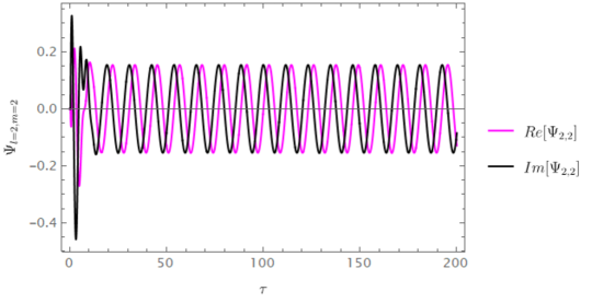
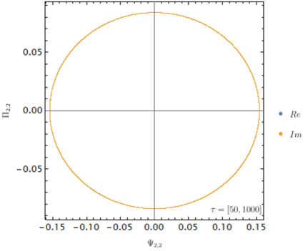
Figure 12: Left: Waveform at $\mathscr{I}^{+}$ of a scalar point-charge on a circular geodesic in a SMBH Schwarzschild background at $\sigma_{p}=2M/6M$ for the $(l,m)=(2,2)$ mode. Right: Here one shows the phase portrait of the numerical evolution for the field $\Psi_{2,2}(\tau,\sigma)$ at $\mathscr{I}^{+}$. One determines a reasonable time to assume all junk radiation to dissipate away and our simulation to be in steady-state to be at least $\tau>50$, corresponding to ignoring the first 1.5 orbits as per the plot on the left.

4 Applications to numerical black hole perturbation theory

To demonstrate further the main application of the DiscoTEX algorithm, particularly with a focus on numerical black hole perturbation theory, one will now briefly demonstrate how the algorithm can be used to calculate the amplitude of the scalar and gravitational self-forces for a point-particle on a circular geodesic in a Schwarzschild black hole. The work here does not investigate the numerical optimisations, this will be subject to upcoming collaborative work [51, 86] and it merely intends to demonstrate the algorithms ability to give highly accurate amplitude results through numerical weak-form solutions via DiscoTEX. Here, in the first section, one will briefly demonstrate this for scalar perturbations and in the next section how weak-form solutions can be recovered for metric perturbation amplitudes and gravitational-self force calculations will be demonstrated. To get a better idea of how the numerical optimisation factors are determined in the context of gravitational self-force applications work one refers the reader to our previous work [49] and first paper of the series [51, 86].

4.1 Modelling perturbations in Schwarzschild via DiscoTEX

Here one will show how key quantities for EMRI modelling can be computed via the DiscoTEX algorithm for when a scalar point-charge, $q$ or a point-particle $\mu$ prescribes a circular geodesic around a SMBH of mass $M$. The SMBH is described by a four-dimensional manifold $\mathcal{M}$, the Schwarzschild spacetime, which in Schwarzschild coordinates, $x^{\mu}=(t,r,\theta,\phi)$ is given as,

$$ds^{2}=-f(r)dt^{2}+f(r)^{-1}dr^{2}+r^{2}d\omega^{2}\ \ \ \ f(r)=\bigg{(}1-\frac{2M}{r}\bigg{)},$$ (176)

with $d\omega^{2}=d\theta^{2}+\sin^{2}\theta\ d\theta d\phi$. In numerical BHPT it is standard to split the spacetime into two sub-manifolds $\mathcal{M}=\mathcal{M}^{2}\times\mathcal{S}^{2}$, where $\mathcal{M}^{2}$ is a Lorentzian sub-manifold with coordinates $x^{a}=(t,r)$ and $\mathcal{S}^{2}$ is a the spherical space described by $\mathcal{S}^{2}$ described by coordinates $\theta^{A}=(\theta,\phi)$.

The point-charge $q$ point-particle $\mu$, has the worldline $x^{\mu}=\big{(}t_{p}(s),r_{p}(s),$ $\theta_{p}(s),\phi_{p}(s)\big{)}$, where $s$ denotes the proper time on the circular geodesic given as $x^{\mu}_{p}=(t_{p},r_{p},\theta=\frac{\pi}{2},\phi_{p})$, with constants of motion

$$\mathcal{E}=\frac{f}{\sqrt{1-3M/r}},\ \mathcal{L}=\frac{\sqrt{rM}}{1-3M/r},\ \Omega_{\phi}=\frac{M}{r^{3}}.$$ (177)

The four velocity $u^{\mu}=dx^{\mu}/ds$ has the components

$$u^{t}=\frac{\mathcal{E}}{f},\ (u^{r})^{2}=\mathcal{E}^{2}-\mathcal{U}^{2},\ u^{\theta}=0,\ u^{\phi}=\frac{\mathcal{L}}{r^{2}},$$ (178)

where $\mathcal{U}^{2}=f(r)+(1+\mathcal{L}/r^{2})$.

4.2 Modelling scalar perturbations in Schwarzschild via DiscoTEX

One starts by demonstrating the usefulness of the algorithms by modelling the behaviour of a scalar point-particle charge $q$ around the SMBHs described by,

$$\square_{g}\Psi=\frac{1}{\sqrt{-\textbf{g}}}\partial_{\mu}[\sqrt{-\textbf{g}}\ g^{\mu\nu}\partial_{\nu}]\Psi=S_{\Psi},$$ (179)

with the determinant of the background SMBH given as $\textbf{g}=-r^{4}\sin^{2}\theta$. The source term associated with the scalar point-charge is given as

$$S_{\Psi} = -4\pi\rho=-4\pi\int\frac{\delta^{4}(x^{\mu}-x^{\mu}_{p}(s))}{\sqrt{-\textbf{g}}}\ ds.$$ (180)

Taking advantage of the spherical symmetry of the SMBH background metric I apply spherical harmonic decomposition expanding the field as

$$\Psi(t,r,\theta,\phi)=\frac{1}{r}\sum^{\infty}_{l,m}\psi^{lm}(t,r)Y^{lm}(\theta,\phi),$$ (181)

and $S_{\Psi}$ as

$$S_{\Psi}=-\frac{4\pi qf}{E}\delta(r-r_{p})Y^{lm}(\theta,\phi)Y^{*lm}(\theta_{p},\phi_{p}),$$ (182)

with the subscript $p$ denoting it is with respect to the particle’s position and where the following Dirac delta propriety to collapse the spherical components,

$$\delta(\theta-\theta_{p})\delta(\phi-\phi_{p})=\sin\theta\sum_{l,m}Y^{lm}(\theta,\phi)Y^{*lm}(\theta_{p},\phi_{p}),$$ (183)

has been used.

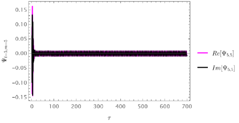
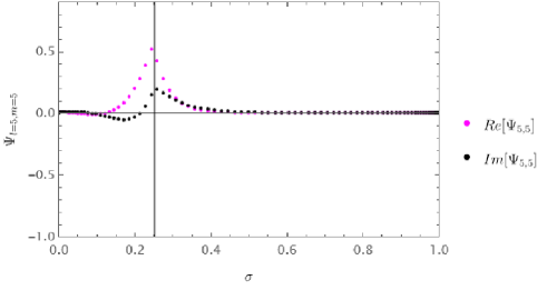
Figure 13: Left: Waveform at $\mathscr{I}^{+}$ of a point-particle on a circular geodesic in a SMBH Schwarzschild background at $\sigma_{p}=2M/7.9456M$ for the $(l,m)=(5,5)$ mode. Right: Here we show the retarded hyperboloidal field $\Psi(\tau\,\sigma)$ at $\sigma_{p}=2M/7.9456M$ and $\tau=500$ extending from the future null infinity $\mathscr{I}^{+}$ at $\sigma=0$ and to the event horizon $\sigma=1$.

Applying these expansions into eq.(179), one gets the $1+1D$ distributional sourced wave-like equation

$$\square\psi=G^{lm}(t,r)\delta(r-r_{p}),$$ (184)

where the source-term is given by

$$G^{lm}(t,r)=-\frac{4\pi f^{2}}{Er}Y^{*lm}(\theta_{p},\phi_{p})$$ (185)

and with the d’Alembert-like wave operator

$$\square=-\frac{\partial^{2}}{\partial t^{2}}+\frac{\partial^{2}}{\partial x^{2}}-V_{l}(r),$$ (186)

with the potential associated with the scalar perturbation given by

$$V_{l}(r)=\frac{f}{r^{2}}\bigg{[}l(l+1)+\frac{2M}{r}\bigg{]}.$$ (187)

For the scalar case, the jumps are given as,

$$[[\psi]]=0,\hskip 11.38092pt{}[[\psi_{r}]]=\frac{G^{lm}(t,r)}{f^{2}}.$$ (188)

To compute the scalar self-force (SSF) the field $\Psi$ shall be regularised as demonstrated in [67]. The first step is to decompose the field into,

$$\Psi^{\text{ret}}=\Psi^{R}+\Psi^{S},$$ (189)

where $\Psi^{S}$ is the singular part of the field equation and $\Psi^{\rm{ret}},\Psi^{R}$ are the retarded and regular fields respectively. The SSF is then given as

$$F_{\alpha}:=q\nabla_{\alpha}\Psi_{R}=q(\nabla_{\alpha}\Psi^{ret}-\nabla_{\alpha}\Psi^{S}).$$ (190)

Furthermore, the computations presented here follow the mode-sum computational strategy as put forward by [87]. The retarded field $\Psi^{\text{ret}}$ is decomposed as

$$\Psi^{\text{ret,l}}_{\alpha}=\nabla_{\alpha}\sum^{l}_{m=-l}\psi^{lm}(t,r)Y^{*lm}(\theta_{p},\phi_{p}).$$ (191)

Here the interest lies in demonstrating the algorithm’s main application so one will only look at the $r-$component. To compute $F_{r}$ one needs to correct for the singular terms contributions as demonstrated by [88],

$$\underset{x^{\mu}\rightarrow x^{\mu}_{p}}{\lim}=q\bigg{[}A_{\alpha}(l(l+1))+B_{\alpha}+\frac{C_{\alpha}}{l+\frac{1}{2}}+...\bigg{]}.$$ (192)

Finally, with substituting Eq.(192) into Eq.(190, 194) one gets

$$F_{lr}=F^{\textrm{ret}\pm}_{lr}-A_{r}(l(l+1))-B_{r}-\sum^{3}_{n=1}F^{l}_{r}[2n],$$ (193)

where

$$F^{\textrm{ret}\pm}_{lr}=\sum^{l}_{m=-l}\partial_{r}\bigg{[}\frac{1}{r}\psi^{l,m}(t,r)\bigg{]}^{\pm}Y^{*lm}(\theta_{p},\phi_{p}).$$ (194)

As emphasised, the goal here is to demonstrate the accuracy and the flexibility of the DiscoTEX (and relatives) algorithm, to that effect one choose to not include the numerical recipe description in detail as it closely follows the previous section but where now the minimal gauge implementation is exactly as described in our previous work in Section III of [49]. The exception here is in the jump implementation which in the scalar case greatly simplifies and can be trivially computed via chain-rules from Eqs.(188). With a preliminary numerical optimisation study The the following optimisation parameters were determined: $N=60$ nodes, $J=12$ jumps, $\Delta\tau=0.05$, and $\tau_{\text{extr}}=10,000$. In Fig.(12) on the left plot the scalar waveforms for the point-particle on a circular geodesic at $r_{p}=6M$ for the $(l,m)=\{2,2\}$ mode are shown. Unlike in the previous section where the exact solutions were used as initial data for the evolution, here, as its usual in BHPT simulations, one has given it trivial initial data [49]. This causes the simulation to be contaminated at earlier times by junk radiation as evidenced on this figure at least during $\tau=[0,10]$, as its customary, the solution is to wait until the simulation reaches steady-state evolution. Aided by the phase portraits given by the plot on the right of Fig.(12) one estimated the minimal time for steady-state evolution to be at least $\tau>50$, at earlier times symplectic structure was not preserved corresponding to about 1.5 orbits. One decided to extract the quantities at a much longer time, $\tau=10,000$ after quick convergence tests showing that the quantities evaluated at the particle limit needed longer times to converge. This value is nevertheless an overestimate, as explained this will be given in detail [51].

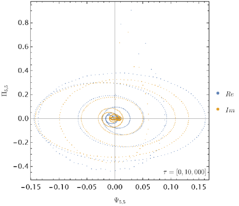
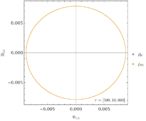
Figure 14: Here we show the phase portrait of our numerical evolution for the field $\Psi^{5,5}(\tau,\sigma)$ at infinity $\mathscr{I}^{+}$. Left: Phase portrait for the entire simulation $\tau=[0,10,000]$. Right: Phase portrait after we waited a sufficiently long-time, $\tau>500$, allowing all junk radiation to dissipate away and our simulation to reach steady-state.

To calculate the $r-$component of the SSF as given by Eq.(194) all is needed is to take the numerical solution obtained by solving Eq.(184) and interpolate at the particle limit via DiscoTEX. One notes Eq.(194) expands as

$$F^{\textrm{ret}\pm}_{lr}=\sum^{l}_{m=-l}\bigg{[}\frac{1}{r}\partial_{r}\psi^{l,m}(t,r)-\frac{1}{r^{2}}\psi^{l,m}(t,r)\bigg{]}^{\pm}Y^{*lm}(\theta_{p},\phi_{p}).$$ (195)

This means one needs, not only to interpolate the field at the particle limit, but also its $r$-derivative. These interpolations are done on the hyperboloidal field $\Psi(\tau,\sigma)$ spanning the spatial domain $\sigma=[0,1]$, with the aid of chain rules between the minimal gauge chart to the Schwzraschild chart i.e $(t\to t(\tau,\sigma),\ r\to r(\sigma))$, which will naturally introduce extra-derivatives. For the SSF one, using the DiscoTEX algorithm, interpolates directly at the hyperboloidal field, $\Psi(\tau,\sigma)$

$$\Psi(\tau,\sigma)\bigg{|}_{\sigma=\sigma_{p}}\approx\sum^{N}_{j=0}\bigg{[}\Psi_{j}(\tau)+\Delta_{\Psi}(\sigma_{j}-\sigma_{p}(\tau);\sigma-\sigma_{p}(\tau))\bigg{]}\pi_{j}(\sigma)\bigg{|}_{\sigma=\sigma_{p}}.$$ (196)

The $r-$derivative by the chain-rule is given as

$$\partial_{r}=-\frac{\sigma^{2}}{2M}\bigg{[}\partial_{\sigma}+\partial_{\sigma}H(\sigma)\partial_{\tau}\bigg{]},$$ (197)

and thus one interpolate at $\Pi(\tau,\sigma)$, which is simply obtained by

$$\Pi(\tau,\sigma)\bigg{|}_{\sigma=\sigma_{p}}\approx\sum^{N}_{j=0}\bigg{[}\Pi_{j}(\tau)+\Delta_{\Pi}(\sigma_{j}-\sigma_{p}(\tau);\sigma-\sigma_{p}(\tau))\bigg{]}\pi_{j}(\sigma)\bigg{|}_{\sigma=\sigma_{p}},$$ (198)

and finally the $\sigma$- derivative of the field, $\partial_{\sigma}\Psi(\tau,\sigma)$ is simply given by

$$\partial_{\sigma}\Psi(\tau,\sigma)\bigg{|}_{\sigma=\sigma_{p}}\approx\sum^{N}_{j=0}\bigg{[}\Psi_{j}(\tau)\pi_{j}^{\prime}(\sigma)$$

$$+\Delta_{\Psi}(\sigma_{j}-\sigma_{p}(\tau);\sigma-\sigma_{p}(\tau))\pi^{\prime}_{j}(\sigma)\bigg{]}\bigg{|}_{\sigma=\sigma_{p}}.$$ (199)

To check the accuracy of DiscoTEX the first 5 modes for the $r-$component of the self-force were computed to get $F_{r}=4.152070\times 10^{-3}$ with a numerical error of $6.0\times 10^{-9}$. One notes the numerical error was calculated against that of [67] and the value is only for the $l=1$ to $l=5$ modes. In upcoming work we will give the full results [51].

4.3 Modelling gravitational perturbations in Schwarzschild via DiscoTEX

To demonstrate the main application of the DiscoTEX algorithm one will use some of the results in [49] (the full results and discussion will be given in [51, 86]) and compute the gravitational perturbations as described by the Regge-Wheeler-Zerilli formalism. Specifically, unlike in [49], where we solved for the Regge-Wheeler and Zerilli master functions [19, 20] as the goal is to compute the self-force as regularised by [20], one will now, for the first time and for completion, solve for the Cunningham-Price-Moncrief (CPM), $\Psi^{a}_{lm}(t,r)$, [89, 90] and Zerilli-Moncrief (ZM) master functions $\Psi^{p}_{lm}(t,r)$, [91] as given in [28, 23, 70].

4.3.1 Phase 1 - Numerical weak-form solution to CPM/ZM master functions via DiscoTEX

The CPM and the ZM satisfy the following wave equation

$$\bigg{[}-\frac{\partial^{2}}{\partial t^{2}}+\frac{\partial^{2}}{\partial x^{2}}-V^{a/p}_{l}(r)\bigg{]}\Psi^{a/p}_{lm}(t,r)=S_{lm}^{a/p}(t,r),$$ (200)

where $x$ remains as the tortoise coordinate. The axial and polar potentials are given as

$$V^{a}_{l}(r)=\frac{1}{r^{2}}\bigg{[}l(l+1)-\frac{6M}{r}\bigg{]},$$ (201)

$$V^{p}_{l}(r)=\frac{1}{\tilde{\Lambda}^{2}}\bigg{[}\mu^{2}\bigg{(}\frac{\mu+2}{r^{2}}+\frac{6M}{r^{3}}\bigg{)}+\frac{36M^{2}}{r^{4}}\bigg{(}\mu+\frac{2M}{r}\bigg{)}\bigg{]},$$ (202)

where $\tilde{\Lambda}:=(l-1)(l+2)+6M/r$ and $\mu:=(l-1)(l+2)$. The source $S_{lm}^{a/p}(t,r)$ is given as,

$$S_{lm}^{a/p}(t,r) = \bar{G}^{a/p}_{lm}(t)\delta\left(r-r_{p}(t)\right)+\bar{F}^{a/p}_{lm}(t)\delta^{\prime}(r-r_{p}(t)).$$

For simplicity, and following [49, 23] I define the source term functions as,

$$\bar{F}_{lm}^{a/p}(t) = F^{a/p}_{lm}(t,r_{p}(t)),$$ (203)

$$\bar{G}_{lm}^{a/p}(t) = \bigg{[}G^{a/p}_{lm}(t,r)-\partial_{r}F^{a/p}_{lm}(t,r)\bigg{]}\bigg{|}_{r=r_{p}}.$$ (204)

The jumps of the retarded field at the particle’s trajectory have been given generically in [49] to facilitate implementation across different versions of the RWZ equations and are given as

$$[[\Psi]](t)=\frac{\mathcal{E}^{2}}{f^{2}_{p}U^{2}_{p}}\bar{F}^{a,p}_{lm}(t),$$ (205)

$${}[[\Psi_{r}]](t)=\frac{E^{2}}{f_{p}^{2}U^{2}_{p}}\bigg{[}\bar{G}^{a,p}_{lm}(t)$$

$$+\frac{1}{U^{2}_{p}r^{2}_{p}}\bigg{(}3M-\frac{\mathcal{L}^{2}}{r_{p}}+\frac{5M\mathcal{L}^{2}}{r^{2}_{p}}\bigg{)}\bar{F}^{a,p}_{lm}(t)-2\dot{r}_{p}\frac{d}{dt}\big{(}[[\Psi]](t)\big{)}\bigg{]},$$ (206)

$$[[\Psi_{t}]](t)\partial_{t}[[\Psi]](t)-\dot{r}_{p}[[\Psi_{r}]](t),$$ (207)

$$[[\Psi_{x}]](t)=f_{p}[[\Psi_{r}]](t).$$ (208)

The reader should now refer to D in this manuscript to get the correct $\bar{G}(t),\bar{F}(t)$ functions. To confirm the accuracy of the solution as done in [49], one evaluates the energy fluxes at infinity $\mathscr{I}^{+}$ and the horizon $\mathcal{H}$, as given by the formulas

$$\dot{E}^{\pm}_{lm}=\frac{1}{64\pi}\frac{(l+2)!}{(l-2)!}\bigg{|}\dot{\Psi}^{\pm}_{lm}(t,r)\bigg{|}^{2},$$ (209)

$$\dot{L}^{\pm}_{lm}=\frac{im}{64\pi}\frac{(l+2)!}{(l-2)!}\bigg{|}\dot{\Psi}^{\pm}_{lm}(t,r)\Psi^{\pm*}_{lm}(t,r)\bigg{|}.$$ (210)

The numerical error associated with the DiscoTEX algorithm is computed by comparing against the frequency domain results as given by the BHPT toolkit [71]. The relative error difference is thus defined as,

$$\eta=\bigg{|}1-\frac{\dot{E}_{\textrm{total}}}{\dot{E}^{\textrm{ref}}_{\textrm{total}}}\bigg{|}.$$ (211)

$(l,m)$	$\dot{E}^{\infty}_{lm}$	$\dot{E}^{\infty,GDS}_{lm}$ [49]	$\dot{L}^{\infty}_{lm}$	$\dot{L}^{\infty,GDS}_{lm}$ [49]
(2,2)	$1.70621955\times 10^{-4}$	$1.70621955\times 10^{-4}$	$3.8214217\times 10^{-3}$	$3.8214217\times 10^{-3}$
(2,1)	$8.16304\times 10^{-7}$	$8.163040\times 10^{-7}$	$1.82828\times 10^{-5}$	$1.8282769\times 10^{-5}$
(3,3)	$2.547061\times 10^{-5}$	$2.547061\times 10^{-4}$	$5.704656\times 10^{-3}$	$5.704656\times 10^{-4}$
(3,2)	$2.5198\times 10^{-7}$	$2.519844\times 10^{-7}$	$5.644\times 10^{-6}$	$5.643699\times 10^{-6}$
(3,1)	$2.1730\times 10^{-9}$	$2.1730\times 10^{-9}$	$4.8669\times 10^{-8}$	$4.86693\times 10^{-9}$
(4,4)	$4.7254\times 10^{-6}$	$4.72538\times 10^{-6}$	$1.0583\times 10^{-4}$	$1.058345\times 10^{-4}$
(4,3)	$5.775\times 10^{-7}$	$5.7749\times 10^{-9}$	$1.29\times 10^{-6}$	$1.29340\times 10^{-9}$
(4,2)	$2.509\times 10^{-9}$	$2.5090\times 10^{-9}$	$5.619\times 10^{-8}$	$5.619\times 10^{-9}$
(4,1)	$8.4\times 10^{-13}$	$8.40\times 10^{-13}$	$1.88\times 10^{-11}$	$1.880\times 10^{-9}$
(5,5)	$9.4555\times 10^{-7}$	$9.4560\times 10^{-7}$	$2.11785\times 10^{-5}$	$2.11785\times 10^{-5}$
(5,4)	$1.23\times 10^{-7}$	$1.232\times 10^{-9}$	$2.76\times 10^{-7}$	$2.760\times 10^{-9}$
(5,3)	$1.093\times 10^{-9}$	$1.093\times 10^{-9}$	$2.448\times 10^{-3}$	$2.448\texttimes\times 10^{-8}$
(5,2)	$2.7\times 10^{-12}$	$2.78\times 10^{-12}$	$6.0\times 10^{-11}$	$6.24\times 10^{-11}$
(5,1)	$1.0\times 10^{-15}$	$1.0\times 10^{-15}$	$2.8\times 10^{-14}$	$3.0\times 10^{-12}$
Total	$2.029077\times 10^{-4}$	$2.0290770\times 10^{-4}$	$4.544526\times 10^{-4}$	$4.5445256\times 10^{-3}$
$\eta$	$1.2\times 10^{-7}$	$3.8\times 10^{-8}$	$1.2\times 10^{-7}$	$2.0\times 10^{-8}$

Table 5: Comparison of energy fluxes at $\mathscr{I}^{+}$, in units of $(M/\mu)^{2}$ against reference FD values comparing to our previous time-domain work [49] which was solving a different set of RWZ equations as described in [19, 20]. These results verify our numerical implementation, the gauge invariance associated of energy and angular momentum fluxes and the equivalency between the different RWZ equations formalisms.

$(l,m)$	$\dot{E}^{\infty}_{lm}$	$\eta$	$\dot{L}^{\infty}_{lm}$	$\eta$
(2,1)	$7.8175\times 10^{-5}$	$4.3\times 10^{-6}$	$1.7688\times 10^{-5}$	$3.5\times 10^{-5}$
(2,2)	$1.64810\times 10^{-4}$	$6.8\times 10^{-7}$	$3.7292\times 10^{-3}$	$1.7\times 10^{-6}$
(3,1)	$2.0883\times 10^{-9}$	$2.5\times 10^{-5}$	$4.725\times 10^{-8}$	$2.6\times 10^{-5}$
(3,2)	$2.3974\times 10^{-7}$	$1.8\times 10^{-5}$	$5.4247\times 10^{-6}$	$1.8\times 10^{-5}$
(3,3)	$2.44440\times 10^{-5}$	$4.1\times 10^{-6}$	$5.5301\times 10^{-4}$	$4.1\times 10^{-6}$

Table 6: Comparison of the energy and angular momentum fluxes at $\mathscr{I}^{+}$ for when the point-particle is at $r_{p}=8M$. The results presented here were obtained with the numerical factors of [80, 81] for comparison and to avoid erroneous implementations of the DiscoTEX algorithm. One too uses, $J=10$ jumps, $N=45$ Chebyshev nodes and a timestep of $\Delta\tau=0.01$. The numerical error was calculated against the frequency-domain results of [71]. See footnote 14.

For consistency and to fairly compare against our work in [49] one has decided to use the same optimisation factors: $N=89$ Chebyshev collocation nodes, $J=11$ jumps, a time-step of $\Delta\tau=0.02$ with the physical quantities extracted at around $\tau=10,000$. It should be stressed implementation of DiscoTEX should always be accompanied by through numerical studies, given the difference in the equations and source terms, with this version and the version in [49] there could be other optimal choices. On the left plot of Fig.(13) one sees the gravitational waveform at $(l,m)=(5,5)$ with the field being highly irregular at earlier times due to the junk radiation. As explained in [49] after waiting a minimal time, steady-state is reached and one observes the expected periodic pattern for a point-particle on a circular geodesic with an angular frequency $m\Omega_{\phi}$, where $\Omega_{\phi}$ is as defined in eq.(177). In Table 5 the energy fluxes are computed for the first 5 modes against previous frequency-domain work [20]. Furthermore, in Table 6, one gives results for $r_{p}=8M$ with numerical optimisation factors $N=45$ Chebyshev nodes, $J=10$ and $\Delta\tau=0.01$ as the solutions to these equations have previously been attempted in the literature by [80, 81] with those optimisation factors (see footnote 14).

4.3.2 Phase 2 and Phase 3 - Numerical weak-form solutions for metric perturbation reconstruction and gravitational self-force computations via DiscoTEX interpolations

In this section one shows how the metric perturbations prescribed by a point-particle on a circular geodesic can be reconstructed and used to compute the conservative gravitational self-force (GSF) through the DiscoTEX algorithm. The results of [49] will be used and, as in the previous section, the intention is merely to demonstrate the algorithm’s main application. The complete results are to be include in upcoming work with collaborators [51, 86].

GSF computations form dissipative laws

As briefly mentioned in Section 1 it is possible to compute the $t$-component of the self-force, $\mathcal{F}_{t}$ by computing the total energy flux radiated into/out of the black hole [92, 93, 94] using the numerical results from Phase I from the previous section for the master functions of RW/Z,

$$\mathcal{F}_{t}=-\frac{1}{2u^{t}}u^{\alpha}u^{\beta}\partial_{t}h_{\alpha\beta}=2\ \ \frac{1}{u^{t}}\frac{d\mathcal{E}}{dt}.$$ (212)

Furthermore $\phi$-component of the gravitational self-force can be further computed, due to helical symmetry present in circular geodesic motion,

$$\dot{\mathcal{E}}_{\text{total}}+\Omega\ \dot{\mathcal{J}}_{\text{total}}=0,$$ (213)

$$\mathcal{F}_{t}+\Omega\ \mathcal{F}_{\phi}=0.$$ (214)

$r_{p}$	$\dot{\mathcal{E}}_{\text{total}}$	$\mathcal{F}_{t}^{lm}$	$\eta$	$\dot{\mathcal{L}}_{\text{total}}$	$\mathcal{F}_{\phi}^{lm}$	$\eta$
$7.9456M$	$2.03294497*10^{-4}$	$3.20775924*10^{-4}$	$1.3*10^{-9}$	$4.5531889267*10^{-3}$	$-7.1844216179*10^{-2}$	$2.9*10^{-11}$

Table 7: Comparison of the gravitational self-force $t-$ component, $\mathcal{F}_{t}$ from our time domain algorithm against state-of-the-art frequency domain results of [20] for the first $l_{max}=20$ modes.

On Table 5 the energy fluxes for the first $l$ modes the self-force components are computed, as $\mathcal{F}_{t}$ and $\mathcal{F}_{\phi}$ and with an unforeseen accuracy of $10^{-9}$/$10^{-11}$ trhough time-domain methods from the direct numerical solution of a distributionally sourced PDE such as eq.(200) showing the power of the DiscoTEX numerical algorithm directly addressing all the three main difficulties highlighted in the introduction.

Conservative GSF computations

As a preview into our upcoming work [51, 86] and for the sake of completion of the numerical algorithm highlighted in Section 3, one will also show how the numerically machinery here can be used to reconstruct the metric and compute the un-regularised gravitational self-force. To compute this, the fields are evaluated at the vicinity of the particle i.e at the particle limit from the right and the left as radiation propagates towards infinity and the horizon of the black hole. For simplicity one chooses to demonstrate DiscoTEX for the odd-component given the equations are not singular as shown in [20]. The results here are computed against the state-of-the-art frequency domain results of [20] transformed to the time-domain case. One does not explicitly give the magnitudes as this is part of upcoming collaborative work [51, 86]. The un-regularised odd-parity self-force is given for Regge-Wheeler and Eazy gauges radiatives modes is the same and one has

$$\mathcal{F}^{r,lm}_{RW/EZ}(r_{p})=\frac{r_{p}f_{p}\Omega}{r_{p}-3M}\bigg{[}\beta+r_{p}\partial_{r}\beta\bigg{]}\partial_{\theta}Y_{lm}\bigg{(}\frac{\pi}{2},\phi_{p}(t)\bigg{)}.$$ (215)

The only required metric perturbation is given as [20, 23]

$$\beta(t,r)=-\frac{1}{\lambda r}\bigg{[}f\Psi^{a}(t,r)+rf\partial_{r}\Psi^{a}(t,r)-r^{3}E_{C}\bigg{]}.$$ (216)

where $\lambda$, $E_{C}$ are constant quantities defined in Appendix B.2 of [49]. Even though this quantity contains a singular term $E_{C}$ one can show by writing it’s weak-form solution that all components are regular and should $vanish$ at the particle, see for example [23]. The weak-form is as given in the Introduction section of this manuscript by Eq.(1). Similarly, one must also calculate the red-shifts as in [20]

$$\Delta U^{r,lm}_{RW/EZ}(r_{p})=\frac{2r_{p}^{2}\Omega}{r_{p}-3M}\beta\ \partial_{\theta}Y_{lm}\bigg{(}\frac{\pi}{2},\phi_{p}(t)\bigg{)}.$$ (217)

For the numerical weak-form solutions here, one chooses to work with Chebyshev collocation nodes due to the significant faster results and comparable accuracy at the particles. The numerical choices are $N=89$ Chebyshev nodes, $J=11$ jumps, and it was found a time of $\tau=400$ with a $\Delta\tau=0.02$ to be sufficient for accurate computations. As demonstrated in the previous sections, one uses the numerical solutions obtained via DiscoTEX with the generic discontinuous interpolator in Eq.(51) and evaluate at the particle position of $\sigma_{p}$,

$$\Psi(\tau,\sigma)\bigg{|}_{\sigma=\sigma_{p}}\approx\sum^{N}_{j=0}\bigg{[}\Psi_{j}(\tau)+\Delta_{\Psi}(\sigma_{j}-\sigma_{p}(\tau);\sigma-\sigma_{p}(\tau))\bigg{]}\pi_{j}(\sigma)\bigg{|}_{\sigma=\sigma_{p}},$$ (218)

Interpolation for the field derivative, necessary for eqs.(215 - 217) computations, follows trivially from this formula,I note though care must be taken when transforming back to the physical quantities from the hyperboloidal ones.

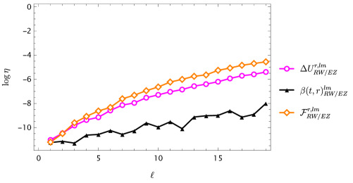
Figure 15: Numerical convergence result for all the un-regularised physically relevant quantities for Phase II and Phase III for the computation of the gravitational self-force in the time domain in the Regge-Wheeler gauge. All $l_{\text{max}}=20$ modes against reference frequency domain values of [20] at $r_{p}=7.9456M$ are given.

In Fig.(15) one demonstrates the numerical results for the first $l=20$ modes for the metric perturbation amplitudes gravitational self-force and redshift amplitudes given as numerical weak-form solutions via DiscoTEX. For all these results the cumulative error for each mode was calculated, and one highlights that, as seen in results of [49] in Section IV, the physical quantities magnitudes and hereby contributions to final results of eq.(215- 217) decrease as the number of $l$ modes increases, and hereby one expects the final error contributions to become less and less significant as we will show in the third paper [86] of the series starting with [49]. The main observation is that the DiscoTEX numerical algorithm is capable of highly accurate computations required for the gravitational self-force programme [16, 18].

4.4 State of numerical algorithms in the time-domain for numerical black hole-perturbation theory applications

Numerical Scheme	Difficulty 1	Difficulty 2	Difficulty 3	Accuracy	Applications
Lousto et al	Finite-difference	RBCs.	EX Finite-difference	Accurate	[REQ 1, 2]
[95]			c. stable, constrained	$2^{nd}$ order	[96, 97, 98, 72]
Lousto et al	Finite-difference	RBCs.	EX Finite-difference	Accurate	[REQ 1,2]
[99]			c. stable, constrained	$4^{rd}$ order	[100, 101]
Sopuerta et al	Finite element	RBCs.	IMEX	Accurate	[REQ 1]
[102, 103]	method		See [103]	$4^{rd}$ order	[103]
Sopuerta et al	Multi-domain	RBCs.	EX RK4	Accurate	[REQ 1,2] [104, 105]
[104]	pseudospectral		c. stable, constrained	$4^{rd}$ order	[106, 107, 108, 109]
Hughes et al	Finite impulse	[110] BCs	EX Lax-Wendroff	Accurate	[REQ 1] [111]
$\delta$-code [112, 113]	representation		c.stable, constrained	$2^{nd}$ order	Sev. [114, 115, 116]
Dolan, Barack	Finite-difference	RBCs.	EX RK4	Accurate	[REQ 1,2] [117, 118]
[119, 120]	Puncture		c. stable, constrained	$4^{rd}$ order	[121]
Dolan	Finite-difference	RBCs.	EX RK4	Accurate	[REQ 1]
[122]			c. stable, constrained	$4^{rd}$ order	[122]
Khana et al	Gaussian approximation	[110] BCs	EX Lax-Wendroff	Accurate	[REQ 1]
[110, 123]	the $\delta$ distribution		c.stable, constrained	$2^{nd}$ order	[124, 125]
Thornburg et al	Finite difference	Pure Outflow BCs	EX RK4	Accurate	[REQ 1,2]
[126]	with	with FD	c.stable, constrained	$4^{rd}$ order	[126]
	Berger-Oliger	ghost-zones	IMEX RK considered	$3^{rd}$ order
	mesh refinement		c.stable, [127, 128, 129]		See App.B11 [126]
Nagar et al	Gaussian approximation	RBCs	EX Lax-Wendroff	Accurate	[REQ 1]
[130]	the $\delta$ distribution		c.stable, constrained	$2^{rd}$ order	[131, 132, 133]
Bernuzzi et al	Gaussian approximation	RBCs	EX RK4	Accurate	[REQ 1]
[134]	the $\delta$ distribution		c.stable, constrained	$4^{rd}$ order
Teukode	Gaussian approximation	hyperboloidal layer	EX RK4	Accurate	[REQ 1]
[84, 135, 136]	the $\delta$ distribution		c.stable, constrained	$4^{rd}$ order	Sev. [137, 138, 139]
Diener et al	$8th$ order	Penalty	EX RK4	Accurate	[140, 141]
[141]	Finite-difference	BCs [142]	c.stable, constrained	$4^{rd}$ order	[REQ 1,2][$1^{st}$ SCE]
Diener et al	Discontinuous	hyperboloidal layer	EX RK4	Highly acc.	[REQ 1]
[143, 144]	Garlerkin		c.stable, constrained	$4^{rd}$ order	[143, 144]
Field et al	Discontinuous	RBCs	EX RK4	Accurate	[REQ 1]
[28, 68]	Garlerkin		c.stable, constrained	$4^{rd}$ order	[28, 68]
Field et al	Discontinuous	hyperboloidal layer	EX RK4	Highly acc.	[REQ 1]
[85]	Garlerkin		c.stable, constrained	$4^{rd}$ order	[85]
DiscoEX	Discontinuous	hyperboloidal slice	EX RK2, RK4	Highly acc.	[REQ 1,2] [47]
[53, 47]	collocation LIP	minimal gauge	c.stable, constrained	$2^{nd}/4^{rd}$ order
DiscoIMP	Discontinuous	RBCs	IM Hermite 2,4	–	[REQ 1,2] [47]
[52, 53, 47]	collocation LIP	–	unconditionally stable
DiscoIMP	Discontinuous	hyperboloidal slice	–	–	[REQ 1,2] [47]
[53, 47]	collocation LIP	minimal gauge			[51, 86]
DiscoTEX	Discontinuous	RBCs	IMTEX Hermite 2,4	–	[REQ 1,2] [47]
[53, 47]	collocation LIP
DiscoTEX	Discontinuous	hyperboloidal slice	–	–	[REQ 1,2]
[53, 47]	collocation LIP	minimal gauge			[49, 51, 86]
Fully-spectral,	Multi-domain	hyperboloidal slice	Spectral IM SDIRK	Highly acc.	[REQ 1,2] [51, 86]
P.Macedo et al [50]	spectral decomposition	minimal gauge	unconditionally stable	$3^{rd}$ order

Table 8: Overview of numerical methods used by the radiation-reaction community for the modelling of EMRIs in the time-domain. Here the short notation, c.stable, refers to conditionally stable.

One of the key goals for the Laser Interferometer Space Antenna (LISA) scheduled for 2034 is the detection of EMRIs. These systems are more likely formed from scattering capture mechanism where the small BH spirals radiatively into the massive BH with high initial eccentricities and a small periastron passage emitting gravitational-wave bursts as they radiatively inspiral until their orbit shrinks and circularises with a very sudden transition from inspiral to plunge. Before it plunges, it will though spend a very long-time in inspiral in the strong-field regime, potentially taking years, making it an exceptionally promising probe for strong-gravity due to the very high signal-to-noise ratio of gravitational wave emission. One of the most promising tests will be the ability to give with high precision measurements, that will allow to test the “no-hair” conjecture, as LISA is expected to be able to measure mass and spin with a precision of $10^{[-3,-6]},10^{[-4,-6]}$ respectively. Furthermore it can help test alternative theories of general relativity by potentially probing extra polarisation modes of gravitational waves and they can also act as dark sirens providing independent measurements for the expansion rate of the Universe [16, 18].

Most of the progress [145, 146, 147] in the modelling of these systems comes from the radiation-reaction programme [16, 18] using the two-timescale expansion in the Fourier domain and hence all current waveform templates are available and generated through this framework. A fully alternative approach is to perform a self-consistent evolution (SCE) in the time-domain where one could simply couple the field-equations and the equations of motion evolving it as a system self-consistently sourcing the orbit by computing the GSF at each time step. So far only [148] has performed this for a toy model describing a scalar charge on a non-rotating background. The SCE under the gravitational self-force, however, has remained a challenge. To understand why, it is important to emphasise a few key proprieties of these physical systems:

• eccentric, spinning, inclined motion;

• long-term slow evolution;

• sudden transition from inspiral to plunge.

These proprieties, along with the aforementioned difficulties $1)-4)$ which must address [REQ 1,2] place clear key constraints on the range of suitable numerical methods. One of the struggles in modelling EMRIs in the Fourier domain, has been handling eccentricity as it requires a high number of modes for convergence which in the time-domain translates to requiring a very small step-size. Another concern comes from $b)$ as it will be a very long-term evolution and hence numerical methods which have their time step-size constrained are likely to fall short. Immediately, these two factors place a clear constraint in the ideal numerical evolution time-integrators used. Most of the progress in the time-domain within the radiation-reaction self-force community, see Table 8, has come from the application of time-step size constrained explicit numerical integrators mostly at $2^{nd}$ and $4^{rd}$ order convergence. As such, time-domain results have usually been significantly less accurate and more computationally expensive then frequency-domain strategies. With the time-steppers, Hermite implicit IM and implicit-turned-explicit IMTEX implemented here with DiscoIMP/DiscoTEX, respectively, it was shown that these issues can be avoided altogether if unconditionally/long-term stable schemes are used. One has shown that highly accurate GSF computations are possible in the time-domain and with competitive accuracy to frequency domain methods. It is also worth to mention, the results in [49] and here were meant to show agreement with the frequency domain approach and hence why one chooses to compute as much as $l=20$ modes. However, careful convergence studies and further gauge of DiscoTEX’s $3$ numerical optimisation factors, i.e number of jumps, nodes, times-step size can result in faster convergence and reduce the required number of modes, as expected in the time-domain, showing exceptional promise for modelling eccentric systems. Furthermore, in future work, we will show the implementation of a fully independent algorithm to DiscoIMP/DiscoTEX , which is fully-spectral and also implements an advanced SDIRK unconditionally stable $3^{th}$ order time-stepper [50] which has registered significantly highly accurate results [51, 86], conserves sympletic structure and it is faster than DiscoTEX.

Altogether, the simplicity of DiscoTEX as evidenced by the evolution algorithms in Eqs.(133, 170), and its remarkable stability and coordinate preserving proprieties make it a well-suited algorithm for the modelling of EMRI systems, and further motivates our current work in modelling the most realistic system where the background black hole is a rotating Kerr BH on eccentric and spinning orbits. It is also noteworthy, the times-steppers here mentioned have the potential to improve any of the other algorithms on Table 8, and it is strongly recommended for more realistic and accurate implementations. Implementation of more adequate time-stepper schemes would also allow for a more fair comparison between the rich choices that were made to address difficulty $1)$ as evidenced by Table 8, the impact here would be multi-disciplinary. Implementation of more suitable strategies to accurately handle boundary conditions has single-handedly already resulted in the improvement of the algorithms used by Bernuzzi and Field as evidence in Table 8, and hence here is recommended that hyperboloidal slices automatically enforcing boundary conditions be used when solving these equations [50, 65, 66, 67].

5 Conclusion

In the body of this work one has presented a numerical scheme, DiscoTEX, which uses discontinuous collocation methods with implicit-turned-explicit IMTEX time-integrator. One has proved that implicit IM and implicit-turned-explicit IMTEX Hermite integrators are capable of preserving symplectic structure, exactly and numerically, while retaining high accuracies and long-term stability for both homogeneous and distributional sourced wave and wave-like equations. One has further demonstrated that IM & IMTEX time integrators, when solving the same problem, are more accurate than traditionally explicit schemes such as Runge-Kutta, (even when writing in optimised Horner-Form), which requires an order-7 scheme to achieve the same accuracy attained with an IMTEX order-2 scheme (lowest order). When applied to the same distributionally sourced problem it was also demonstrated that DiscoTEX achieves the same accuracies as DiscoIMP while being faster, retaining stability and coordinate-preserving proprieties and less cumbersome to implement.

Furthermore, this work gives and compares implementations of the IMTEX Hermite time-integration scheme and the discontinuous time-integration rule up to $12th$ orders and justifies our decision to use an order-4 scheme in [49] and upcoming work [47, 51, 86]. The stagnation in accuracy results from the increase in round-off error associated with the increase of the evolution matrices complexity and increase in the number of operations. These results could potentially be improved with the use of compensation-summation for example to reduce round-off error. Increase in the precision used in the operations prior to the computation of the evolution algorithm, for example given in Eq.(133), also results in a significant improvement of these results at the expense of extra computational time. Future work will improve on this and explore these results further.

Here one presents the work in [53, 47] and previously discussed in [54, 46] for simpler toy models and give the numerical studies that led to the final form of the algorithm one implemented in [49, 51, 86]. Furthermore this work solves three issues: $i)$ It fully verifies the recurrence relation, for the first time given in Eq.(104- 106), initially given in [52], proving the algorithm numerically and exactly with comparisons against existing exact solutions to distributionally sourced wave-equations [28, 68] and implementations in either coordinate charts $(t,x)$ and $(\tau,\sigma)$; $ii)$ It demonstrates and proves, that highly accurate computations are possible both at the particle and it’s right and left-limits, by using the numerical solution provided by the DiscoTEX solver through generic interpolation; $iii)$ It demonstrates there are no losses in accuracy when implementing an hyperboloidal slice nor when using an Implicit-turned-explicit IMTEX instead of an implicit scheme; $iv)$ One further demonstrated by applying DiscoTEX to both distributionally sourced wave-like equations governing the scalar and gravitational perturbations describing an EMRI problem that highly accurate computations are possible, with ease, in the time-domain. An overview of the requirements for successful modelling of EMRIs through a time-evolution is also provided and complemented with an overview of all previous numerical methods utilised within the radiation-reaction community which highly influenced the results at the time on Table 8.

Finally, one has shown it is possible to compute the required quantities for modelling of EMRIs with high accuracies that comfortably surpass the requirements for detection by LISA[18]. In this work the focus was on demonstrating how the DiscoTEX (and DiscoIMP) numerical machinery is applied, however in previous work [49] and future work one will demonstrate the full computations for the scalar and gravitational perturbations of point-particle on a Schwarzschild background BH [51, 86]. Additionally in future work, we will include an alternative solution with a fully independent numerical scheme which is fully-spectral, developed by Panosso Macedo [50] which not only implements a state-of-the-art [50] implicit integrator and hence retains the necessary unconditionally stability proprieties for successful evolutions of EMRIs, it has the benefit of not requiring higher order jumps. A back of the envelop calculation, estimates DiscoTEX/ DiscoIMP/ DiscoEX [53, 47] to require a high number of jumps, say 10 $(l,m)$ modes are necessary, by applying the formula $N_{\rm{evolution}}=((l_{\rm{max}}+1)(l_{\rm{\max}}+2))/2$, one estimates a total number of $J_{\rm{total}}=J_{max}*N_{\rm{evolution}}=726$ jumps to be necessary, where $J_{\rm{max}}=11$ jumps as in this work and [49]. This further estimates the computational cost of my simulations, it is likely this method will always be slower than our fully-spectral implementation however effective use of high performance computing can significantly attenuate the cost as the evolution algorithm is relatively simple to implement and reduced to mostly vector-matrix and matrix-matrix multiplications. In future work one will explore implementations across different architectures. Particularly, in future work we will show how both the hyperboloidal DiscoTEX, (with extra comparisons via DiscoIMP/DiscoEX) and the fully-spectral implicit scheme can be used as tools to achieve this with the required accuracies for detection by LISA [18] for both non-rotating Schwarzschild [51, 86] and rotating Kerr black holes. This work [53, 47], our results in [49, 50] and our collaborative incoming work [51, 86] in the time-domain offers promising new prospects for the modelling of EMRIS. Particularly it provides a clear avenue for the first full alternative generation waveform model to current strategies relying of the two-time scale expansion in the Fourier domain through a self-consistent evolution.

Appendix A Complementary work to Section 3.2

Note that the following section is from [49] and it has been included here for completeness. This is my own PhD original work [53] and will appear in [47].

A.1 Jump condition derivation through the Frobenius Method

As explained in [49] one reconsiders Eq.(7) by transforming the d’Alembert operator $\square\Psi$ back to it’s pre-tortoise coordinate transformation $(t,r)$ form, reverting eq.(29) into a PDE of the form,

$$-\frac{\partial^{2}\Psi}{\partial t^{2}}+\eta(r)\frac{\partial^{2}\Psi}{\partial r^{2}}+\varrho(r)\frac{\partial\Psi}{\partial r}-V_{l}(r)\Psi=S_{lm}(t,r),\ \ \ \$$ (219)

where $\eta(r)=f^{2}$, $\rho(r)=ff^{\prime}$.
One will at the end of deriving our recurrence relation for $J_{m+2}(t)$ then revert back to its tortoise coordinate form, which is slightly different yet trivially the same as it’s been previously done in the literature [103, 28, 23]. The numerical algorithm here can be seen as an application of the Frobenius method [151, 152] for the case where we have a function in weak form. One will therefore revisit it briefly here. The Frobenius method states if $x_{0}$ is an ordinary point of an ODE describing a smooth function $\Phi(x)$ we can expand it in a Taylor series about $x_{0}$. A Maclaurin series by taking the expansion point as $x_{0}=0$, resulting in

$$\Phi=\sum_{n=0}^{\infty}a_{n}x^{n}.$$ (220)

Plugging $\Phi$ back in the ODE and group the coefficients by power. One then obtains a recurrence relation for the $nth$ term and write the series expansion in terms of the $a_{n}$ coefficients. It’s relevant to the calculations that follow to highlight the first two derivatives, for convenience one lists:

$$\Phi =\sum_{n=0}^{\infty}a_{n}x^{n}.$$ (221)

$$\Phi^{\prime} =\partial_{x}\bigg{(}\sum_{n=0}^{\infty}a_{n}x^{n}\bigg{)},$$ (224)

$$=\sum_{n=1}^{\infty}na_{n}x^{n-1},$$

$$=\sum_{n=0}^{\infty}(n+1)a_{n+1}x^{n}.$$

$$\Phi^{\prime\prime} =\partial_{x}^{2}\bigg{(}\sum_{n=0}^{\infty}a_{n}x^{n}\bigg{)},$$ (227)

$$=\sum_{n=2}^{\infty}n(n-1)a_{n}x^{n-2},$$

$$=\sum_{n=0}^{\infty}(n+2)(n+1)a_{n+2}x^{n}.$$

A.1.1 Unit Jump relations

As given in Section 2, the wave and wave-like distributional sourced equations studied here assume a weak-form as described by Eq. (8). One can also write the ansatz:

$$\Psi_{lm}(t,r)=\Psi^{S}_{lm}(t,r)+\Psi^{J}_{lm}(t,r),$$ (228)

where $\Psi^{S}_{lm}(t,r)$ like $\Psi^{+/-}(t,r)$ functions in Eq. (8) are smooth functions satisfying everywhere the homogeneous PDE,

$$-\frac{\partial^{2}\Psi^{S}}{\partial t^{2}}+\eta(r)\frac{\partial^{2}\Psi^{S}}{\partial r^{2}}+\varrho(r)\frac{\partial\Psi^{S}}{\partial r}-V_{l}(r)\Psi^{S}=0,$$ (229)

and $\Psi^{J}_{lm}(t,r)$ describe the inhomogeneous part of the master function in an infinite series as with the Frobenius method. One then writes,

$$\Psi^{J}(r,t;r_{p}(t))=\sum^{\infty}_{n=0}J_{n}(t)\Psi_{n}(r;r_{p}(t)).$$ (230)

where $\Psi_{n}$ are piecewise monomials centred at the discontinuity $r=r_{p}(t)$:

$$\Psi_{n}\big{(}r,t;r_{p}(t)\big{)}=\Psi_{n}\big{(}r-r_{p}(t)\big{)}=$$

$$=\Psi_{n},=\frac{1}{2}\text{sgn}\big{(}r-r_{p}(t)\big{)}\frac{\big{(}r-r_{p}(t)\big{)}^{n}}{n!},$$ (231)

here the sgn is the signum function. The expansion in Eq. (230) allows one to compute the discontinuities,

$$\frac{\partial^{m}\Psi}{\partial{r}^{m}}\bigg{|}_{r=r_{p}^{+}}-\frac{\partial^{m}\Psi}{\partial{r}^{m}}\bigg{|}_{r=r_{p}^{-}} = \frac{\partial^{m}\Psi^{J}}{\partial{r}^{m}}\bigg{|}_{r=r_{p}^{+}}-\frac{\partial^{m}\Psi^{J}}{\partial{r}^{m}}\bigg{|}_{r=r_{p}^{-}}=J_{m}(t).$$ (232)

These functions have the property that all spatial derivatives have matching left and right limits at $r=r_{p}(t)$,

$$\frac{\partial^{m}\Psi_{n}}{\partial{r}^{m}}\bigg{|}_{r=r_{p}^{+}}-\frac{\partial^{m}\Psi_{n}}{\partial{r}^{m}}\bigg{|}_{r=r_{p}^{-}}=\delta_{m,n},$$ (233)

except at the $nth$ derivative, where one has a jump of one.

$$\frac{\partial^{n}\Psi_{n}}{\partial{r}^{n}}\bigg{|}_{r=r_{p}^{+}}-\frac{\partial^{n}\Psi_{n}}{\partial{r}^{n}}\bigg{|}_{r=r_{p}^{-}}=1.$$ (234)

By differentiating the monomial one obtains,

$$\frac{\partial\Psi_{n}}{\partial r}=\left\{\begin{array}[]{ccc}\Psi_{n-1}&\text{for}&n\geq 1\\ \delta(w)&\text{for}&n=0\end{array}\right..$$ (235)

$$\frac{\partial^{2}\Psi_{n}}{\partial r^{2}}=\left\{\begin{array}[]{ccc}\Psi_{n-2}&\text{for}&n\geq 2\\ \delta(w)&\text{for}&n=1\\ \delta^{\prime}(w)&\text{for}&n=0\end{array}\right..$$ (236)

One notes that here for simplicity, $w=(r-r_{p}(t))$ is introduced. The idea to use unit jump functions to compute higher order jumps was given by [153] who initially demonstrated it for the wave equation sourced by a Dirac $\delta$ distribution as showed in [52].

A.1.2 Spatial Jumps

The inhomogeneous part of the solution is given by Eq. (230). To determine the jumps in Eq. (219), it is useful to find the spatial and temporal derivatives of the unit jump functions. These derivations are an application of the Frobenius method. More explicitly, one has for the first order derivative of Eq. (230):

$$\partial_{r}\Psi^{J}(w)=\partial_{r}\bigg{[}\sum^{\infty}_{n=0}\bigg{(}J_{n}(t)\Psi_{n}(w)\bigg{)}\bigg{]},$$ (237)

$$=\sum^{\infty}_{n=1}\bigg{(}J_{n}(t)\Psi_{n-1}(w)\bigg{)},$$

$$=\sum^{\infty}_{n=0}\bigg{(}J_{n+1}(t)\Psi_{n}(w)\bigg{)}+J_{0}(t)\delta(w).\ \ \ \ \ \ \ \$$ (238)

where the selection property of Dirac-$\delta$ as given by Eq. (262) was used to ensure the problem is fully with respect to the the particle’s worldline, $r_{p}(t)$. For second order one then has,

$$\partial_{r}^{2}\Psi(w) = \partial_{r}^{2}\bigg{[}\sum^{\infty}_{n=0}\bigg{(}J_{n}(t)\Psi_{n}(w)\bigg{)}\bigg{]},$$

$$= \sum^{\infty}_{n=0}\bigg{[}J_{n+2}(t)\Psi_{n}(w)\bigg{]}+J_{1}(t)\delta(w)+J_{0}(t)\delta^{\prime}(w).$$

Given the coefficients present in the differential operators in Eq. (219) and the potential term it is important to revisit Eq. (231). One of it’s key properties is

$$\text{sgn}=\frac{x}{|x|}=\frac{|x|}{x}.$$ (240)

Using this one re-writes Eq. (231) as

$$\Psi_{n} = \frac{1}{2}\frac{|w|}{w}\frac{w^{n}}{n!},$$ (241)

$$= \frac{1}{2n!}(w)^{n-1}|w|,$$ (242)

$$|w|\Psi_{n} = \frac{1}{2n!}|w|w^{n}.$$ (243)

One can then generalise this for $\Psi_{n+m}$:

$$\Psi_{n+m}(w) = \frac{1}{(n+m)!}\big{|}w\big{|}\big{(}w\big{)}^{n+m-1},$$ (244)

$$\Psi_{n+m}(w)(n+m)! = \frac{\big{|}w\big{|}\big{(}w\big{)}^{n+m-1}}{2}.\ \ \$$ (245)

Substituting for the term $|w|\ w^{n}/2$ in the RHS of this equation by the LHS of Eq. (243) multiplied by $n!$ one get,

$$n!\ (w)\Psi_{n} = (w)^{1-m}(n+m)!\Psi_{n+m},$$

$$(w)(w)^{m-1}\Psi_{n} = \frac{(m+n)!}{n!}\Psi_{n+m},$$

$$(w)^{m}\Psi_{n} = \frac{(m+n)!}{n!}\Psi_{n+m}.$$ (246)

One wants to be able to expand any coefficient in $r$ acting on our master functions $\Psi^{a/p}_{lm}(t,r)$ and its differential operators as given by Eq. (219). As an example let’s consider the potential term $V_{l}(r)$ acting on the master function, one can expand it around $r=r_{p}$

$$V_{l}(r)=\sum^{\infty}_{k=0}V^{(k)}_{l}(r_{p})\frac{(r-r_{p})^{k}}{k!},$$ (247)

where $k\leq n$ and compute the product $V(r)\Psi^{J}(r;r_{p})$ following the ansatz of Eq. (230),

$$V_{l}(r)\Psi^{J}(r;r_{p})=\bigg{[}\sum^{\infty}_{k=0}V^{(k)}_{l}(r_{p})\frac{(r-r_{p})^{k}}{k!}\bigg{]}\times\bigg{[}\sum^{\infty}_{n=0}J_{n}(t)\Psi_{n}(r;r_{p})\bigg{]}.\ \$$ (248)

Furthermore, given $k\leq n$ we can define $n=m-k$ where at $n=0$, $m=k$, and the preceding equation simplifies to,

$$V_{l}(r)\Psi^{J}(r;r_{p})=\sum^{\infty}_{k=0}\sum^{\infty}_{m=k}V_{l}^{(k)}(r_{p})$$

$$\times\frac{(r-r_{p})^{k}}{k!}J_{m-k}(t)\Psi_{m-k}(r;r_{p}).$$ (249)

From Eq. (246) with $m=k$ and $n=m-k$ one has,

$$(r-r_{p})^{k}\Psi_{m-k}=\frac{(m-k+k)!}{(m-k)!}\Psi_{m-k+k},$$

$$(r-r_{p})^{k}\Psi_{m-k}=\frac{m!}{(m-k)!}\Psi_{m}.$$ (250)

Eq. (249) then simplifies to,

$$V_{l}(r)\Psi^{J}(r;r_{p})=\sum^{\infty}_{m=0}\sum^{m}_{k=0}V_{l}^{(k)}(r_{p})\frac{m!}{(m-k)!k!}J_{m-k}(t)\Psi_{m}(r;r_{p})$$

$$=\sum^{\infty}_{m=0}\bigg{[}\sum^{m}_{k=0}{m\choose k}V_{l}^{(k)}(r_{p})J_{m-k}(t)\bigg{]}\Psi_{m}(r;r_{p}),$$ (251)

where to go from the first to the second line factorial notation is adapted. Furthermore one extends this to the coefficients of the first order derivative of the master functions as given by Eq. (238),

$$\varrho(r)\partial_{r}\Psi(w)=\sum^{\infty}_{m=0}\bigg{[}\sum^{m}_{k=0}\varrho^{(k)}(r_{p}){m\choose k}J_{m+1-k}(t)\Psi_{m}(w)\bigg{]}$$

$$+\varrho(r_{p})J_{0}(t)\delta(w).$$ (252)

Furthermore for the second-order jump one has, Eq. (LABEL:spatial_o2_fb),

$$\eta(r)\partial_{r}^{2}\Psi(w)=\sum^{\infty}_{m=0}\bigg{[}\sum^{m}_{k=0}\eta^{(k)}(r_{p}){m\choose k}J_{m+2-k}(t)\Psi_{m}(w)\bigg{]}$$

$$+\eta(r)J_{1}(t)\delta(w)+\eta(r)J_{0}(t)\delta^{\prime}(w),$$

$$=\sum^{\infty}_{m=0}\bigg{[}\sum^{m}_{k=0}\eta^{(k)}(r_{p}){m\choose k}J_{m+2-k}(t)\Psi_{m}(w)\bigg{]}$$

$$+\eta(r_{p})J_{1}(t)\delta(w)+\eta(r_{p})J_{0}(t)\delta^{\prime}(w)$$

$$-2\varrho(r_{p})J_{0}(t)\delta(w),$$ (253)

For both derivations selection properties as given by Eqs. ((262),  (263)) were applied on the coefficient of the Dirac delta distribution and its $r$-derivative respectively, to go from the second to the third line.

A.1.3 Temporal Jumps

The first order temporal derivative and associated jumps of the function $\Psi^{J}(r,t;r_{p})$ are:

$$\partial_{t}\Psi^{J}(w)=\partial_{t}\sum^{\infty}_{m=0}\bigg{[}J_{m}(t)\Psi_{m}(w)\bigg{]},$$

$$=\sum^{\infty}_{m=0}\bigg{[}\dot{J}_{m}(t)-\dot{r}_{p}J_{m+1}(t)\bigg{]}\Psi_{m}(w)$$

$$-\dot{r_{p}}J_{0}(t)\delta(r-r_{p}).$$ (254)

The second order derivative can be obtained by calculating:

$$\partial_{t}^{2}\Psi^{J}(w)=\partial_{t}\bigg{[}\sum^{\infty}_{m=0}\dot{J}_{m}(t)\Psi_{m}(w)\bigg{]}-$$

$$\partial_{t}\bigg{[}\sum^{\infty}_{m=0}\dot{r_{p}}J_{m+1}(t)\Psi(w)\bigg{]}-\partial_{t}\bigg{[}\dot{r_{p}}J_{0}\delta(w)\bigg{]}.$$ (255)

For simplicity and to clarify one will be showing the explicit calculation this derivatives as $D1,D2,D3$ given respectively as,

$$D1=\partial_{t}\bigg{[}\sum^{\infty}_{m=0}\dot{J}_{m}(t)\Psi_{m}\bigg{]}=\sum^{\infty}_{m=0}\bigg{[}\ddot{J}_{m}(t)$$

$$-\dot{r}_{p}\dot{J}_{m+1}\bigg{]}\Psi_{m}(w)-\dot{r_{p}}\dot{J}_{0}\delta(w),$$ (256)

followed by,

$$D2=-\partial_{t}\bigg{[}\sum^{\infty}_{m=0}J_{m+1}(t)\dot{r}_{p}\Psi(w)\bigg{]}$$

$$=\sum^{\infty}_{m=0}\bigg{(}-\dot{r}_{p}\dot{J}_{m+1}(t)-\ddot{r}_{p}J_{m+1}(t)+\dot{r}_{p}^{2}J_{m+2}(t)\bigg{)}\Psi_{m}(w)$$

$$+\dot{r}_{p}^{2}J_{1}(t)\delta(w),$$ (257)

and finally by,

$$D3=-\bigg{[}\bigg{(}\dot{r}_{p}\dot{J}_{0}+\ddot{r}_{p}J_{0}(t)\bigg{)}\delta(w)-\dot{r}_{p}^{2}J_{0}\delta^{\prime}(w)\bigg{]}$$

$$=r_{p}^{2}J_{0}(t)\delta^{\prime}(w)-\dot{r}_{p}\dot{J}_{0}(t)\delta(w)$$

$$-\ddot{J}_{0}(t)\delta(w).$$ (258)

Plugging this results into Eq. (A.1.3) one obtains:

$$\partial^{2}_{t}\Psi^{J}(w)=\sum^{\infty}_{m=0}\bigg{[}\ddot{J}_{m}(t)-2\dot{r}_{p}\dot{J}_{m+1}(t)-\ddot{r}_{p}J_{m+1}(t)+\dot{r}_{p}^{2}J_{m+2}(t)\bigg{]}\psi_{m}(w)$$

$$+\dot{r}_{p}^{2}J_{1}(t)\delta(w)-2\dot{r}_{p}\dot{J}_{0}(t)\delta(w)-\ddot{J}_{0}(t)\delta(w)+r_{p}^{2}J_{0}(t)\delta^{\prime}(w)$$ (259)

Matching coefficients in $\delta^{\prime}(w)$ with respect to the particle worldline gives the first initialising jump,

$$J_{0}(t)=\frac{F^{a/p}_{lm}(t,r_{p})}{\big{(}f^{2}_{p}-\dot{r}_{p}^{2}\big{)}}.$$ (260)

Similarly for the second and final initialising jump one matchs the coefficients of the Dirac $\delta(z)$,

$$J_{1}(t)=-2\dot{r}_{p}\partial_{t}J_{0}(t)-\big{(}\ddot{r}_{p}-f_{p}f^{\prime}_{p}\big{)}J_{0}(t)$$

$$+\big{[}G^{a/p}_{lm}(t,r_{p})-\partial_{r_{p}}F^{a/p}_{lm}(t,r_{p})\big{]}/\big{(}f^{2}_{p}-\dot{r}_{p}^{2}\big{)}.$$ (261)

These jumps match the documented jumps in the literature [28, 23] without the $f$ factor and equations given in Eq. (205, 206) which match and follow the approach of [23]. One could then to calculate the higher order jumps collect all remainder terms by solving for $J_{m+2}(t)$ as given in Eq.(54).

A.2 Dirac delta distribution proprieties

In this work the following selection proprieties are used

$$f(a)\delta(a-b)=f(b)\delta(b-a),$$ (262)

$$f(a)\delta^{\prime}(a-b)=f(b)\delta^{\prime}(a-b)-f(b)\delta(b-a).$$ (263)

Furthermore, the following composition rules were also needed:

$$\delta(f(a))=\frac{1}{|f^{\prime}(b)|}\delta(a-b),\ \ \$$ (264)

$$\delta^{\prime}(f(a))=\frac{f^{\prime}(b)}{|f^{\prime}(b)|^{3}}\delta^{\prime}(a-b)+\frac{f^{\prime\prime}(b)}{|f^{\prime}(b)|^{3}}\delta(a-b).\ \ \$$ (265)

where the last distribution was brought to my attention from Appendix F of [154].

Appendix B Complementary work on time-integrators such as Hermite, Hermite IMTEX, HF IMTEX and EX HF RK and discontinuous time-integrators as presented in Section 3.3

B.1 Higher-order IMTEX time integration

Here one gives the explicit equations for all Hermite Horner-Form implicit-turned-explicit HF IMTEX time-integrators derived as explained in 3.3.1 through Eqs.(60, 70) from second- to twelve-order:

Hermite order-2, IMTEX HFH2,

$$\textbf{U}_{n+1}=\textbf{U}_{n}+(\Delta t\ \textbf{L})\cdot\textbf{HFH2}\cdot\textbf{U}_{n},$$ (266)

$$\textbf{HFH2}=\bigg{(}\textbf{I}-\frac{\Delta t}{2}\textbf{L}\bigg{)}^{-1}.$$ (267)

Hermite order-4, IMTEX HFH4,

$$\textbf{U}_{n+1}=\textbf{U}_{n}+\textbf{A}\cdot\textbf{HFH4}\cdot\textbf{U}_{n},$$ (268)

$$\textbf{HFH4}=\bigg{(}\textbf{I}-\frac{\textbf{A}}{2}\cdot\bigg{(}\textbf{I}-\frac{\textbf{A}}{6}\bigg{)}\bigg{)}^{-1},$$ (269)

where here $(\Delta t\ \textbf{L})=\textbf{A}$, $(\Delta t\ \textbf{L})\cdot(\Delta t\ \textbf{L})=\textbf{A}^{2}=\textbf{A}\cdot\textbf{A}$.

Hermite order-8 IMTEX HFH8,

$$\textbf{U}_{n+1}=\textbf{U}_{n}+\textbf{A}\cdot\bigg{(}\textbf{I}+\frac{1}{42}\textbf{A}^{2}\bigg{)}\cdot\textbf{HFH8}\cdot\textbf{U}_{n},$$ (270)

$$\textbf{HFH8}=\bigg{(}\textbf{I}+\textbf{A}\cdot\bigg{(}-\frac{\Delta t}{2}+\textbf{A}\cdot\bigg{(}\frac{3}{28}\textbf{I}+\bigg{(}-\frac{1}{84}\textbf{I}+\frac{\textbf{A}}{1680}\bigg{)}\cdot\textbf{A}\bigg{)}\bigg{)}\bigg{)}^{-1}.$$ (271)

Hermite order-10 IMTEX HFH10,

$$\textbf{U}_{n+1}=\textbf{U}_{n}+\textbf{A}\cdot\bigg{(}\textbf{I}+\textbf{A}^{2}\cdot\bigg{(}\textbf{A}\cdot\bigg{(}\frac{1}{36}\textbf{I}+\frac{\textbf{A}}{15120}\bigg{)}\bigg{)}\bigg{)}\cdot\textbf{HFH10}\cdot\textbf{U}_{n},$$ (272)

$$\textbf{HFH10}=\bigg{(}\textbf{I}+\textbf{A}\cdot\bigg{(}-\frac{1}{2}\textbf{I}+\textbf{A}\cdot\bigg{(}\frac{1}{9}\textbf{I}+$$

$$\textbf{A}\cdot\bigg{(}-\frac{1}{72}\textbf{I}+\bigg{(}\frac{1}{1008}\textbf{I}-\frac{\textbf{A}}{30240}\bigg{)}\cdot\textbf{A}\bigg{)}\bigg{)}\bigg{)}\bigg{)}\bigg{)}^{-1}.$$ (273)

Hermite order-12 IMTEX HFH12,

$$\textbf{U}_{n+1}=\textbf{U}_{n}+\textbf{A}\cdot\bigg{(}\textbf{A}^{2}\cdot\bigg{(}\frac{1}{33}\textbf{I}+\frac{\textbf{A}^{2}}{7920}\bigg{)}\bigg{)}\cdot\textbf{HFH12}\cdot\textbf{U}_{n},$$ (274)

$$\textbf{HFH12}=\bigg{(}\textbf{I}+\textbf{A}\cdot\bigg{(}-\frac{1}{2}\textbf{I}+\textbf{A}\cdot\bigg{(}\frac{5}{44}\textbf{I}+$$

$$\textbf{A}\cdot\bigg{(}\textbf{A}\cdot\bigg{(}-\frac{1}{66}\textbf{I}+\textbf{A}\cdot\bigg{(}\frac{1}{792}\textbf{I}+\bigg{(}-\frac{1}{15840}\textbf{I}+\frac{(\textbf{A})}{665280}\bigg{)}\cdot\textbf{A}\bigg{)}\bigg{)}\bigg{)}\bigg{)}\bigg{)}\bigg{)}^{-1}.$$ (275)

B.2 Explicit Horner-Form Runge-Kutta EX RK time integration schemes

To complement the results showed in Section 3.3.1 one gives the time-integration Explicit Runge-Kutta numerical schemes in Horner-form EX HF RK from second- to sixth-order:

Runge-Kutta order-2, EX HF RK2:

$$\textbf{U}_{n+1}=\textbf{U}_{n}+(\textbf{HFRK2}-\textbf{I})\cdot\textbf{U}_{n},$$ (276)

$$\textbf{HFRK2}=\textbf{I}+\bigg{(}\textbf{I}+\frac{\textbf{A}}{2}\bigg{)}\cdot\textbf{A}.$$ (277)

Runge-Kutta order-3, EX HF RK3:

$$\textbf{U}_{n+1}=\textbf{U}_{n}+(\textbf{HFRK3}-\textbf{I})\cdot\textbf{U}_{n},$$ (278)

$$\textbf{HFRK3}=\textbf{I}+\textbf{A}\cdot\bigg{(}\textbf{I}+\bigg{(}\frac{1}{2}\textbf{I}+\frac{1}{6}\textbf{A}\bigg{)}\cdot\textbf{A}\bigg{)}.$$ (279)

Runge-Kutta order-4, EX HF RK4:

$$\textbf{U}_{n+1}=\textbf{U}_{n}+(\textbf{HFRK4}-\textbf{I})\cdot\textbf{U}_{n},$$ (280)

$$\textbf{HFRK4}=\textbf{I}+\textbf{A}\cdot\bigg{(}\textbf{I}+\textbf{A}\cdot\bigg{(}\frac{1}{2}\textbf{I}+\bigg{(}\frac{1}{6}\textbf{I}+\frac{1}{4}\textbf{A}\bigg{)}\cdot\textbf{A}\bigg{)}.$$ (281)

Runge-Kutta order-5, EX HF RK5:

$$\textbf{U}_{n+1}=\textbf{U}_{n}+(\textbf{HFRK5}-\textbf{I})\cdot\textbf{U}_{n},$$ (282)

$$\textbf{HFRK5}=\textbf{I}+\textbf{A}\cdot\bigg{(}\textbf{I}+\textbf{A}\cdot\bigg{(}\frac{1}{6}\textbf{I}+\bigg{(}\frac{1}{24}\textbf{I}+\frac{1}{120}\textbf{A}\bigg{)}\cdot\textbf{A}\bigg{)}.$$ (283)

Runge-Kutta order-6, EX HF RK6:

$$\textbf{U}_{n+1}=\textbf{U}_{n}+(\textbf{HFRK6}-\textbf{I})\cdot\textbf{U}_{n},$$ (284)

$$\textbf{HFRK6}=\textbf{I}+\textbf{A}\cdot\bigg{(}\textbf{I}+\textbf{A}\cdot+$$

$$\bigg{(}\frac{1}{2}\textbf{I}+\textbf{A}\cdot\bigg{(}\frac{1}{6}\textbf{I}+\textbf{A}\cdot\bigg{(}\frac{1}{24}\textbf{I}+\bigg{(}\frac{1}{120}\textbf{I}+\frac{1}{720}\textbf{A}\bigg{)}\cdot\textbf{A}\bigg{)}\bigg{)}\bigg{)}\bigg{)}.$$ (285)

B.3 IMTEX time-integrator proprieties

In this section the aim is to demonstrate that the Hermite IMTEX algorithm discussed in this manuscript and in previous collaborative work [48, 49] preserves energy and sympletic structure both exactly and numerically, along with its Horner-form counterpart i.e Hermite HF IMTEX. For simplicity one, will demonstrate this by using the simple Hamiltonian as an example, however the proofs here hold for any quadratic Hamiltonian. Generically one has the following canonical equations,

$$\begin{cases}\displaystyle\dot{q}=\frac{dq}{dt}=\frac{\partial H}{\partial p}=\nabla_{p}H,\\ \displaystyle\dot{p}=\frac{dp}{dt}=-\frac{\partial H}{\partial q}=-\nabla_{q}H.\end{cases}$$ (286)

Energy conserving time-integrators

In most cases, and in the body of this work, the Hamiltonian corresponds, physically, to the total energy of a system.. Discretising these derivatives from an $nth$ to $(n+1)th$ step as,

$$\frac{q_{n+1}-q_{n}}{\Delta t}=\frac{H(p_{n+1},q_{n})-H(p_{n},q_{n})}{p_{n+1}-p_{n}},$$ (287)

$$\frac{p_{n+1}-p_{n}}{\Delta t}=\frac{H(p_{n+1},q_{n})-H(p_{n+1},q_{n+1})}{q_{n+1}-q_{n}},$$ (288)

and solving them as a system of equations one has,

$$H(p_{n+1},q_{n+1})-H(p_{n},q_{n})=0,$$ (289)

demonstrating eqs.(287, 288) conserve the Hamiltonian exactly. Thus one defines, that a time integrator is said to conserve energy exactly if

$$H(p_{n+1},q_{n+1})=H(p_{n},q_{n}),$$ (290)

for every smooth Hamiltonian $H(p,q)$.

Symplectic time-integrators

One defines a time-integrator to be sympletic if for every smooth Hamiltonian such as $H(p,q)$ and every step-size $h$ the mapping [56],

$$u_{h}:\Re^{2d}\rightarrow\Re^{2d},\hskip 11.38092ptu_{h}:(p_{n},q_{n})\rightarrow(p_{n+1},q_{n+1}),$$ (291)

is sympletic, meaning its Jacobian matrix,

$$U_{h}:=\bigg{[}\frac{\partial u_{h}(p_{n},q_{n})}{\partial p_{n}}\frac{\partial u_{h}(p_{n},q_{n})}{\partial q_{n}}\bigg{]},$$ (292)

is sympletic for all $h$ i.e, $U^{T}_{h}JU_{h}=J$ for all $h$.

Symmetric time-integrators
A numerical one-step method advancing the solution from $t_{n}$ to $t_{n+1}$, i.e $u_{n+1}=U_{h}(u_{n})$ is symmetric or time-reversible if [56],

$$U_{h}\circ U_{-h}=\textnormal{id}\quad\textnormal{or equivalently,}\quad U_{h}=U^{-1}_{-h},$$ (293)

where id is the identity map. Using the adjoint method definition, $U^{*}_{h}=U^{-1}_{-h}$, the requirement for symmetry/time-reversibility is $U_{h}=U^{*}_{h}$. Thus, a time-integrator is symmetric if under the exchange $u_{n}\leftrightarrow u_{n+1}$ and $h\leftrightarrow-h$ it remains unaltered. Furthermore, it follows, a symmetric time-integrator is $\rho-$ reversible if,

$$\rho\circ U_{h}=U_{-h}\circ\rho,$$ (294)

then the discrete flow $U_{h}$ is a $\rho-$reversible map if and only if $U_{h}$ is a symmetric/time-reversible time-integrator.

One will now proof that Hermite IMTEX schemes conserve both energy and sympletic structure exactly while being symmetric. For simplicity, one considers the simple harmonic oscillator given as,

$$H(p,q)=\frac{1}{2}(p^{2}+q^{2}).$$ (295)

Rewriting eq.(286), following eq.(29), as a reduced system of ODEs in matrix form one has,

$$\frac{d\textbf{U}}{dt}=\textbf{L}\ \textbf{U},$$ (296)

where ,

$$\textbf{U}=\begin{pmatrix}p\\ q\end{pmatrix},\qquad\textbf{L}=\begin{pmatrix}0&-1\\ 1&0\end{pmatrix}.$$ (297)

For all the proofs, for simplicity, one considers IMTEX Hermite schemes of solely order-2 given as,

$$\bigg{[}\textbf{I}-\frac{\Delta t}{2}\textbf{L}\bigg{]}\cdot\textbf{U}_{n+1}=\bigg{[}\textbf{I}+\frac{\Delta t}{2}\textbf{L}\bigg{]}\cdot\textbf{U}_{n},$$

$$\textbf{U}_{n+1}=\bigg{[}\textbf{I}-\frac{\Delta t}{2}\textbf{L}\bigg{]}^{-1}\cdot\bigg{[}\textbf{I}+\frac{\Delta t}{2}\textbf{L}\bigg{]}\cdot\textbf{U}_{n},\ \ \$$ (298)

and in its HF IMTEX form,

$$\textbf{U}_{n+1}=\textbf{U}_{n}+(\Delta t\ \textbf{L})\cdot\textbf{HFH2}\cdot\textbf{U}_{n},$$ (299)

$$\textbf{HFH2}=\bigg{(}\textbf{I}-\frac{\Delta t}{2}\textbf{L}\bigg{)}^{-1}.$$ (300)

All that follows, nevertheless, trivially extends to higher orders.

B.3.1 Hermite IMTEX and HF IMTEX as energy-preserving schemes

Expanding Eq.(298) with the terms as defined for the harmonic oscillator in Eq.(297) one has,

$$\begin{pmatrix}q^{n+1}\\ p^{n+1}\end{pmatrix}=\begin{bmatrix}-1+\frac{8}{4+\Delta t^{2}}&\frac{4\Delta t}{4+\Delta t^{2}}\\ -\frac{4\Delta t}{4+\Delta t^{2}}&-1+\frac{8}{4+\Delta t^{2}}\end{bmatrix}\cdot\begin{pmatrix}q_{n}\\ p_{n}\end{pmatrix},$$ (301)

subtracting both sides by $q_{n}$ and $p_{n}$ and dividing the equations by $\Delta t$ one gets,

$$\frac{q_{n+1}-q_{n}}{\Delta t}=\frac{1}{\Delta t}\bigg{[}-2+\frac{8}{4+\Delta t^{2}}\bigg{]}q_{n}+\frac{4\Delta t}{4+\Delta t^{2}}p_{n}$$ (302)

$$\frac{p_{n+1}-p_{n}}{\Delta t}=\frac{1}{\Delta t}\bigg{[}-2+\frac{8}{4+\Delta t^{2}}\bigg{]}p_{n}-\frac{4\Delta t}{4+\Delta t^{2}}q_{n}.$$ (303)

As evidenced by Eqs.(287, 288) one can establish the equality,

$$\frac{1}{\Delta t}\bigg{[}-2+\frac{8}{4+\Delta t^{2}}\bigg{]}q_{n}+\frac{4\Delta t}{4+\Delta t^{2}}p_{n}=\frac{H(p_{n+1},q_{n})-H(p_{n},q_{n})}{p_{n+1}-p_{n}},$$ (304)

$$\frac{1}{\Delta t}\bigg{[}-2+\frac{8}{4+\Delta t^{2}}\bigg{]}p_{n}-\frac{4\Delta t}{4+\Delta t^{2}}q_{n}=\frac{H(p_{n+1},q_{n})-H(p_{n+1},q_{n+1})}{q_{n+1}-q_{n}}.$$ (305)

Defining for simplicity $c_{1}=(-2+8/4+\Delta t^{2})$ and $c_{2}=4/4+\Delta t^{2}$, one has,

$$\frac{1}{\Delta t}c_{1}^{2}p_{n}q_{n}-c_{2}c_{1}q_{n}^{2}+c_{2}c_{1}p_{n}^{2}-\Delta tc_{2}^{2}p_{n}q_{n}=H(p_{n+1},q_{n})-H(p_{n},q_{n}),$$ (306)

$$\frac{1}{\Delta t}c_{1}^{2}p_{n}q_{n}-c_{2}c_{1}q_{n}^{2}+c_{2}c_{1}p_{n}^{2}-\Delta tc_{2}^{2}p_{n}q_{n}=H(p_{n+1},q_{n})-H(p_{n+1},q_{n+1}),$$ (307)

Now to assess HF IMTEX Eq.(299) is expanded with the terms as defined for the harmonic oscillator in Eq.(297), this gives

$$\begin{pmatrix}q^{n+1}\\ p^{n+1}\end{pmatrix}=\begin{pmatrix}q_{n}\\ p_{n}\end{pmatrix}+\begin{bmatrix}\frac{-\Delta t^{2}}{2(1+\frac{\Delta t^{2}}{4})}&\frac{\Delta t}{1+\frac{\Delta t^{2}}{4}}\\ -\frac{\Delta t}{1+\frac{\Delta t^{2}}{4}}&\frac{-\Delta t^{2}}{2(1+\frac{\Delta t^{2}}{4})}\end{bmatrix}\cdot\begin{pmatrix}q_{n}\\ p_{n}\end{pmatrix},$$ (308)

this yields,

$$\begin{pmatrix}q^{n+1}\\ p^{n+1}\end{pmatrix}=\begin{bmatrix}-1+\frac{8}{4+\Delta t^{2}}&\frac{4\Delta t}{4+\Delta t^{2}}\\ -\frac{4\Delta t}{4+\Delta t^{2}}&-1+\frac{8}{4+\Delta t^{2}}\end{bmatrix}\cdot\begin{pmatrix}q_{n}\\ p_{n}\end{pmatrix},$$ (309)

which is precisely eq.(301) and hereby one concludes HF IMTEX exactly conserve energy too.

B.3.2 Hermite IMTEX and HF IMTEX as sympletic schemes

Calculating the determinant of Eq.(301) pertaining to the Hermite IMTEX scheme one gets,

$$\textrm{det}\ \textbf{U}_{\texttt{IMTEX H2}}=\bigg{(}-1+\frac{8}{4+\Delta t^{2}}\bigg{)}^{2}+\bigg{(}\frac{4\Delta t}{4+\Delta t^{2}}\bigg{)}^{2}=1.$$ (310)

Thus, the required condition for symplecticity holds, to further verify that $\textbf{U}_{\texttt{IMTEX H2}}$ is symplectic one tests,

$$U^{T}_{h}JU_{h}=\begin{pmatrix}-1+\frac{8}{4+\Delta t^{2}}&\frac{\Delta t}{1+\frac{\Delta t^{2}}{4}}\\ -\frac{\Delta t}{1+\frac{\Delta t^{2}}{4}}&-1+\frac{8}{4+\Delta t^{2}}\end{pmatrix}\cdot J\cdot\begin{pmatrix}-1+\frac{8}{4+\Delta t^{2}}&-\frac{\Delta t}{1+\frac{\Delta t^{2}}{4}}\\ \frac{\Delta t}{1+\frac{\Delta t^{2}}{4}}&-1+\frac{8}{4+\Delta t^{2}}\end{pmatrix}$$

$$=J.$$ (311)

By eq.(309) Hermite HF IMTEX also conserves sympletic structure exactly.

B.4 Discontinuous time integration via Hermite and IMTEX interpolation formulae

B.4.1 Solution to the right $p_{+}(t)$ and $p_{-}(t)$ polynomials

By solving the algebraic system highlighted in Section 3 one gets the following right and left polynomials,

$$p_{+}(t)=-\frac{(t-t_{\nu+1})^{3}(6t^{2}+10t_{\nu}^{2}-5t_{\nu}t_{\nu+1}+t_{\nu+1}^{2}+3t(-5t_{\nu}+t_{\nu+1}))}{\Delta t^{5}}f_{\nu}$$

$$+\frac{(t-t_{\nu})^{3}(6t^{2}+3tt_{\nu}+t_{\nu}^{2}-5(3t+t_{\nu})t_{\nu+1}+10t_{\nu+1}^{2})}{\Delta t^{5}}f_{\nu+1}$$

$$-\frac{(t-t_{\nu})(t-t_{\nu+1})^{3}(3t-4t_{\nu}+t_{\nu+1})}{\Delta t^{4}}f^{\prime}_{\nu}$$

$$-\frac{(t-t_{\nu})^{3}(t-t_{\nu+1})(3t-4t_{\nu+1}+t_{\nu})}{\Delta t^{4}}f^{\prime}_{\nu+1}$$

$$-\frac{(t-t_{\nu})^{2}(t-t_{\nu+1})^{3}}{2\Delta t^{3}}f^{\prime\prime}_{\nu}+\frac{(t-t_{\nu})^{3}(t-t_{\nu+1})^{2}}{2\Delta t^{3}}f^{\prime\prime}_{\nu+1}$$

$$-\frac{(t-t_{\nu+1})^{3}(6t^{2}+10t_{\nu}^{2}-5t_{\nu}\ t_{\nu+1}+t_{\nu+1}^{2}+3t(-5t_{\nu}+t_{\nu+1}))}{\Delta t^{5}}\textbf{J}_{0}$$

$$-\frac{(t-t_{\nu+1})^{3}(6t_{\nu}^{3}+t(-8t_{\nu}^{2}-5t_{\nu}(t_{\nu+1}-3t_{\times}t_{\nu+1}(t_{\nu+1}-3t_{\times})))+}{\Delta t^{5}}$$

$$\times\frac{3t^{2}(t_{\nu}+t_{\nu+1}-2t_{\times})-(10t_{\nu}^{2}-5t_{\nu}t_{\nu+1}+t_{\nu+1}^{2})t_{\times})}{\Delta t^{5}}\textbf{J}_{1}$$

$$-\frac{(t-t_{\nu+1})^{3}(3t_{\nu}^{3}(t_{\nu}+t_{\nu+1})-12t_{\nu}^{3}t_{\times}+(10t_{\nu}^{2}-5t_{\nu}t_{\nu+1}+t_{\nu+1}^{2})t_{\times}^{2}+}{2\Delta t^{5}}$$

$$\times\frac{t^{2}(t_{\nu}^{2}+4t_{\nu}t_{\nu+1}+t_{\nu+1}^{2}-6(t_{\nu}+t_{\nu+1})t_{\times}+6t_{\times}^{2})+t(-3t_{\nu}^{2}(t_{\nu}+3t_{\nu+1})+}{2\Delta t^{5}}$$

$$\times\frac{2(8t_{\nu}^{2}+5t_{\nu}t_{\nu+1}-t_{\nu+1}^{2})t_{\times}+3(t_{\nu+1}-5t_{\nu})t_{\times}^{2}))}{2\Delta t^{5}}\textbf{J}_{2}$$

$$-\frac{(t-t_{\nu+1})^{3}\Delta t_{\times}(t_{\nu}^{4}+4t_{\nu}^{3}(t_{\nu+1}-2t_{\times})+3t^{2}(t_{\nu+1}-2t_{\times})+}{6\Delta t^{5}}$$

$$\times\frac{3t^{2}(t_{\nu+1}-2t_{\times})(t_{\nu+1}-t_{\times}+t_{\nu+1}^{2}+3tt_{\nu+1}t_{\times}(t_{\times}-t_{\nu+1})+}{6\Delta t^{5}}$$

$$\times\frac{t_{\nu}(3t^{2}(t_{\nu+1}-t_{\times})-3t(t_{\nu+1}-5t_{\times})(t_{\nu+1}-t_{\times})+t_{\nu+1}(t_{\nu+1}-5t_{\times})t_{\times})}{6\Delta t^{5}}$$

$$\times\frac{+t_{\nu}^{2}(t_{\nu+1}^{2}-5t_{\nu+1}t_{\times}+10t_{\times}^{2}+9t(-t_{\nu+1}+t_{\times})))}{6\Delta t^{5}}\textbf{J}_{3}$$

$$-\frac{(t-t_{\nu+1})^{3}\Delta t_{\times}^{2}(3t_{\nu}^{2}t_{\nu+1}(t_{\nu}+t_{\nu+1})+6t^{2}(t_{\nu+1}-t_{\times})^{2}}{24\Delta t^{5}}$$

$$\times\frac{2t_{\nu}(-2t_{\nu}^{2}-5t_{\nu}t_{\nu+1}+t_{\nu+1}^{2})t_{\times}+(10t_{\nu}^{2}-t_{\nu}t_{\nu+1}+t_{\nu+1}^{2})t_{\times}^{2}}{24\Delta t^{5}}$$

$$\times\frac{t(t_{\nu}^{3}-t_{\nu}(2t_{\nu+1}-5t_{\times})(4t_{\nu+1}-3t_{\times})+t_{\nu}^{2}(-5t_{\nu+1}+2t_{\times})}{24\Delta t^{5}}$$

$$\times\frac{+t_{\nu+1}t_{\times}(-4t_{\nu+1}+3t_{\times})))}{24\Delta t^{5}}\textbf{J}_{4}$$

$$+\frac{(t-t_{\nu+1})^{3}\Delta t_{\times}^{3}(6t_{\nu}^{2}t_{\nu+1}^{2}+3t_{\nu}t_{\nu+1}(-5t_{\nu}+t_{\nu+1})t_{\times}}{120\Delta t^{5}}$$

$$+\frac{(10t_{\nu}^{2}-5t_{\nu}t_{\nu+1}+t_{\nu+1}^{2})t_{\times}^{2}+t^{2}(t_{\nu}^{2}-5t_{\nu}t_{\nu+1}+10t_{\nu+1}^{2}+}{120\Delta t^{5}}$$

$$\times\frac{2t_{\nu}(-2t_{\nu}^{2}-5t_{\nu}t_{\nu+1}+t_{\nu+1}^{2})t_{\times}+(10t_{\nu}^{2}-t_{\nu}t_{\nu+1}+t_{\nu+1}^{2})t_{\times}^{2}}{120\Delta t^{5}}$$

$$\times\frac{3(t_{\nu}-5t_{\nu+1})t_{\times}+6t_{\times}^{2}+t(2t_{\nu}(t_{\nu}-5t_{\nu+1})t_{\nu+1}+)}{120\Delta t^{5}}$$

$$\times\frac{(-5t_{\nu}+34t_{\nu}t_{\nu+1}-5t_{\nu+1})t_{\times}+3(-5t_{\nu}+t_{\nu+1})t_{\times}^{2}))}{120\Delta t^{5}}\textbf{J}_{5}$$ (312)

$$p_{-}(t)=-\frac{(t-t_{\nu+1})^{3}(6t^{2}+10t_{\nu}^{2}-5t_{\nu}t_{\nu+1}+t_{\nu+1}^{2}+3t(-5t_{\nu}+t_{\nu+1}))}{\Delta t^{5}}f_{\nu}$$

$$+\frac{(t-t_{\nu})^{3}(6t^{2}+3tt_{\nu}+t_{\nu}^{2}-5(3t+t_{\nu})t_{\nu+1}+10t_{\nu+1}^{2})}{\Delta t^{5}}f_{\nu+1}$$

$$-\frac{(t-t_{\nu})(t-t_{\nu+1})^{3}(3t-4t_{\nu}+t_{\nu+1})}{\Delta t^{4}}f^{\prime}_{\nu}$$

$$-\frac{(t-t_{\nu})^{3}(t-t_{\nu+1})(3t-4t_{\nu+1}+t_{\nu})}{\Delta t^{4}}f^{\prime}_{\nu+1}$$

$$-\frac{(t-t_{\nu})^{2}(t-t_{\nu+1})^{3}}{2\Delta t^{3}}f^{\prime\prime}_{\nu}+\frac{(t-t_{\nu})^{3}(t-t_{\nu+1})^{2}}{2\Delta t^{3}}f^{\prime\prime}_{\nu+1}$$

$$-\frac{(t-t_{\nu+1})^{3}(6t^{2}+3tt_{\nu}+t_{\nu}^{2}-5(3t+t_{\nu})t_{\nu+1}+10t_{\nu+1}^{2})}{\Delta t^{5}}\textbf{J}_{0}$$

$$-\frac{(t-t_{\nu+1})^{3}(6t_{\nu+1}^{3}+3t^{2}(t_{\nu}+t_{\nu+1}-2t_{\times})-(t_{\nu}^{2}-5t_{\nu}t_{\nu+1}+10t_{\nu+1}^{2})t_{\times}}{\Delta t^{5}}$$

$$\times\frac{+t(t_{\nu}^{2}-5t_{\nu}t_{\nu+1}-8t_{\nu+1}^{2}-3t_{\nu}t_{\times}+15t_{\nu+1}t_{\times}))}{\Delta t^{5}}\textbf{J}_{1}$$

$$-\frac{(t-t_{\nu+1})^{3}(3t_{\nu}^{3}(t_{\nu+1}+t_{\nu+1})-12t_{\nu+1}^{3}t_{\times}+(10t_{\nu}^{2}-5t_{\nu}t_{\nu+1}+10t_{\nu+1}^{2})t_{\times}^{2}+}{2\Delta t^{5}}$$

$$\times\frac{t^{2}(t_{\nu}^{2}+4t_{\nu}t_{\nu+1}+t_{\nu+1}^{2}-6(t_{\nu}+t_{\nu+1})t_{\times}+6t_{\times}^{2})+t(-3t_{\nu}^{2}(3t_{\nu}+t_{\nu+1})+}{2\Delta t^{5}}$$

$$\times\frac{-2(t_{\nu}^{2}-5t_{\nu}t_{\nu+1}-8t_{\nu+1}^{2})t_{\times}+3(t_{\nu}-5t_{\nu+1})t_{\times}^{2}))}{2\Delta t^{5}}\textbf{J}_{2}$$

$$-\frac{(t-t_{\nu+1})^{3}(t_{\nu+1}-t_{\times})(t_{\nu+1}^{2}(t_{\nu}^{2}+4t_{\nu}t_{\nu+1}+t_{\nu+1}^{2})}{6\Delta t^{5}}$$

$$\times\frac{-3t^{2}\Delta t_{\times}(t_{\nu}+t_{\nu+1}-2t_{\times})+t_{\nu+1}(t_{\nu}^{2}-5t_{\nu}t_{\nu+1}-8t_{\nu+1}^{2})t_{\times}+}{6\Delta t^{5}}$$

$$\times\frac{(t_{\nu}^{2}-5t_{\nu}t_{\nu+1}+10t_{\nu+1}^{2})t_{\times}^{2}+3t\Delta t_{\times}(t_{\nu+1}(3t_{\nu+1}-5t_{\times})+t_{\nu}(t_{\nu+1}+t_{\times}))}{6\Delta t^{5}}\textbf{J}_{3}$$

$$\times\frac{(t-t_{\nu})^{3}(t_{\nu+1}-t_{\times})^{2}(3t_{\nu}t_{\nu+1}^{2}(t_{\nu}+t_{\nu+1})+6t^{2}\Delta t_{\times}^{2}+}{24\Delta t^{5}}$$

$$\times\frac{t(-4t_{\nu}^{2}(2t_{\nu+1}+t_{\times})+t_{\nu+1}(t_{\nu+1}-3t_{\times})(t_{\nu+1}+5t_{\times})+}{24\Delta t^{5}}$$

$$\times\frac{t_{\nu}(-5t_{\nu+1}^{2}+26t_{\nu+1}t_{\times}+3t_{\times}^{2})}{24\Delta t^{5}}\textbf{J}_{4}$$

$$+\frac{(t-t_{\nu})^{3}(t_{\nu+1}-t_{\times})^{3}(10t_{\nu+1}^{2}t_{\times}^{2}-5t_{\nu}t_{\nu++1}t_{\times}(3t_{\nu+1}+t_{\times})+}{120\Delta t^{5}}$$

$$+\frac{t_{\nu}^{2}(6t_{\nu+1}^{2}+3t_{\nu+1}t_{\times}+t_{\times}^{2})+t^{2}(10t_{\nu}^{2}+t_{\nu+1}^{2}+3t_{\nu+1}t_{\times}+6t_{\times}^{2}}{120\Delta t^{5}}$$

$$+\frac{-5t_{\nu}(t_{\nu+1}+3t_{\times}))+t(-t_{\nu}^{2}(3t_{\nu+1}+t_{\times})}{120\Delta t^{5}}$$

$$+\frac{-5t_{\nu+1}t_{\times}(t_{\nu+1}+3t_{\times})+t_{\nu}(3t_{\nu+1}^{2}+34t_{\nu+1}t_{\times}+3t_{\times}^{2}))}{120\Delta t^{5}}\textbf{J}_{5}$$

B.4.2 Higher order discontinuous time integration schemes

As per Section 3.3.2 one has the following discontinuous time-integration rules from orders $2$ to $12$,

$$f(t)_{\texttt{NDH2}}=\frac{\Delta t}{2}\bigg{(}f(t_{n})+f(t_{n+1})\bigg{)}+\textbf{J}_{\texttt{H2}}(\Delta t_{\times},\Delta t),$$ (314)

$$f(t)_{\texttt{NDH4}}=\frac{\Delta t}{2}\bigg{(}f(t_{n})+f(t_{n+1})\bigg{)}+\frac{\Delta t^{2}}{12}\bigg{(}\dot{f}(t_{n})-\dot{f}(t_{n+1})\bigg{)}$$

$$+\textbf{J}_{\texttt{H4}}(\Delta t_{\times},\Delta t),$$ (315)

$$f(t)_{\texttt{NDH8}}=\frac{\Delta t}{2}\bigg{(}f(t_{n})+f(t_{n+1})\bigg{)}+\frac{3}{28}\Delta t^{2}\bigg{(}\dot{f}(t_{n})-\dot{f}(t_{n+1})\bigg{)}$$

$$+\frac{\Delta t^{3}}{84}\bigg{(}\ddot{f}(t_{n})+\ddot{f}(t_{n+1})\bigg{)}+\frac{\Delta t^{4}}{1680}\bigg{(}\frac{d^{3}f(t_{n})}{dt^{3}}-\frac{d^{3}{f}(t_{n+1})}{dt^{3}}\bigg{)}$$

$$+\textbf{J}_{\texttt{H8}}(\Delta t_{\times},\Delta t),\ \ \ \$$ (316)

$$f(t)_{\texttt{NDH10}}=\frac{\Delta t}{2}\bigg{(}f(t_{n})+f(t_{n+1})\bigg{)}+\frac{\Delta t^{2}}{9}\bigg{(}\dot{f}(t_{n})-\dot{f}(t_{n+1})\bigg{)}$$

$$+\frac{\Delta t^{3}}{72}\bigg{(}\ddot{f}(t_{n})+\ddot{f}(t_{n+1})\bigg{)}+\frac{\Delta t^{4}}{1008}\bigg{(}\frac{d^{3}f(t_{n})}{dt^{3}}-\frac{d^{3}{f}(t_{n+1})}{dt^{3}}\bigg{)}$$

$$+\frac{\Delta t^{5}}{30240}\bigg{(}\frac{d^{4}f(t_{n})}{dt^{4}}+\frac{d^{4}{f}(t_{n+1})}{dt^{4}}\bigg{)}$$

$$+\textbf{J}_{\texttt{H10}}(\Delta t_{\times},\Delta t),\ \ \ \$$ (317)

$$f(t)_{\texttt{NDH12}}=\frac{\Delta t}{2}\bigg{(}f(t_{n})+f(t_{n+1})\bigg{)}+\frac{5\Delta t^{2}}{44}\bigg{(}\dot{f}(t_{n})-\dot{f}(t_{n+1})\bigg{)}$$

$$+\frac{\Delta t^{3}}{66}\bigg{(}\ddot{f}(t_{n})+\ddot{f}(t_{n+1})\bigg{)}+\frac{\Delta t^{4}}{792}\bigg{(}\frac{d^{3}f(t_{n})}{dt^{3}}-\frac{d^{3}{f}(t_{n+1})}{dt^{3}}\bigg{)}$$

$$+\frac{\Delta t^{5}}{15840}\bigg{(}\frac{d^{4}f(t_{n})}{dt^{4}}+\frac{d^{4}{f}(t_{n+1})}{dt^{4}}\bigg{)}+\frac{\Delta t^{6}}{665280}\bigg{(}\frac{d^{5}f(t_{n})}{dt^{5}}-\frac{d^{5}{f}(t_{n+1})}{dt^{5}}\bigg{)}$$

$$+\textbf{J}_{\texttt{H12}}(\Delta t_{\times},\Delta t),\ \ \ \$$ (318)

where $\textbf{J}_{\texttt{H2-H12}}(\Delta t_{\times},\Delta t)$ are given respectively as,

$$\textbf{J}_{\texttt{H2}}(\Delta t_{\times},\Delta t)=\frac{1}{2}(\Delta t-2\Delta t_{\times})\textbf{J}_{0}+\frac{\Delta t_{\times}}{2}(\Delta t_{\times}-\Delta t)\textbf{J}_{1},$$ (319)

$$\textbf{J}_{\texttt{H4}}(\Delta t_{\times},\Delta t)=\frac{1}{2}(\Delta t-2\Delta t_{\times})\textbf{J}_{0}+\frac{\Delta t_{\times}^{2}}{12}(\Delta t^{2}-6\Delta t\Delta t_{\times}+6\Delta t_{\times}^{2})\textbf{J}_{1}$$

$$-\frac{1}{12}\Delta t_{\times}(\Delta t^{2}-3\Delta t\Delta t_{\times}+2\Delta t_{\times}^{2})\textbf{J}_{2}+\frac{1}{24}\Delta t_{\times}^{2},(\Delta t-\Delta t_{\times})\textbf{J}_{3}\ \ \ \ \ \ \ \$$ (320)

$$\textbf{J}_{\texttt{H8}}(\Delta t_{\times},\Delta t)=\frac{1}{2}(\Delta t-2\Delta t_{\times})\textbf{J}_{0}+\frac{1}{28}(3\Delta t^{2}-14\Delta t\Delta t_{\times}+14\Delta t_{\times}^{2})\textbf{J}_{1}+$$

$$+\frac{1}{84}(\Delta t-2\Delta t_{\times})(\Delta t^{2}-7\Delta t\Delta t_{\times}+7\Delta t_{\times}^{2})\textbf{J}_{2}$$

$$-\frac{1}{1680}(\Delta t^{4}-20\Delta t^{3}\Delta t_{\times}+90\Delta t^{2}\Delta t_{\times}^{2}-140\Delta t\Delta t_{\times}^{3}+70\Delta t_{\times}^{4})\textbf{J}_{3}$$

$$-\frac{1}{1680}(\Delta t-2\Delta t_{\times})(\Delta t-\Delta t_{\times})\Delta t_{\times}(\Delta t^{2}-7\Delta t\Delta t_{\times}+7\Delta t_{\times}^{2})\textbf{J}_{4}$$

$$+\frac{1}{10080}(\Delta t-\Delta t_{\times})^{2}\Delta t_{\times}^{2}(3dt^{2}-14\Delta t\Delta t_{\times}+14\Delta t_{\times}^{2})\textbf{J}_{5}$$

$$-\frac{1}{10080}(\Delta t-2\Delta t_{\times})(\Delta t-\Delta t_{\times})^{3}\Delta t_{\times}^{3}\textbf{J}_{6}+\frac{1}{40320}(\Delta t-\Delta t_{\times})^{4}\Delta t_{\times}^{4}\textbf{J}_{7},\hskip 34.1433pt$$ (321)

$$\textbf{J}_{\texttt{H10}}(\Delta t_{\times},\Delta t)=\frac{1}{2}(\Delta t-2\Delta t_{\times})\textbf{J}_{0}+\frac{1}{18}(\Delta t-3\Delta t_{\times})(2\Delta t-3\Delta t_{\times})$$

$$+\frac{1}{72}(\Delta t-2\Delta t_{\times})(\Delta t^{2}-6\Delta t\Delta t_{\times}+6\Delta t_{\times}^{2})\textbf{J}_{2}$$

$$+\frac{1}{1008}(\Delta t^{4}-14\Delta t^{3}\Delta t_{\times}+56\Delta t^{2}\Delta t_{\times}^{2}-84\Delta t\Delta t_{\times}^{3}+42\Delta t_{\times}^{4})\textbf{J}_{3}$$

$$-\frac{1}{30240}(\Delta t-2\Delta t_{\times})(\Delta t^{4}-28\Delta t^{3}\Delta t_{\times}+154\Delta t^{2}\Delta t_{\times}^{2}-252\Delta t\Delta t_{\times}^{3}+126\Delta t_{\times}^{4})\textbf{J}_{4}$$

$$+\frac{1}{30240}(\Delta t-\Delta t_{\times})\Delta t_{\times}(\Delta t^{4}-14\Delta t^{3}\Delta t_{\times}+56\Delta t^{2}\Delta t_{\times}^{2}-84\Delta t\Delta t_{\times}^{3}+42\Delta t_{\times}^{4})\textbf{J}_{5}$$

$$+\frac{1}{60480}(\Delta t-2\Delta t_{\times})(\Delta t-\Delta t_{\times})^{2}\Delta t_{\times}^{2}(\Delta t^{2}-6\Delta t\Delta t_{\times}+6\Delta t_{\times}^{2})\textbf{J}_{6}$$

$$-\frac{1}{362880}(\Delta t-3\Delta t_{\times})(2\Delta t-3\Delta t_{\times})(\Delta t-\Delta t_{\times})^{3}\Delta t_{\times}^{3}\textbf{J}_{7}$$

$$+\frac{1}{725760}(\Delta t-2\Delta t_{\times})(\Delta t-\Delta t_{\times})^{4}\Delta t_{\times}^{4}\textbf{J}_{8}-\frac{1}{3628800}(\Delta t-\Delta t_{\times})^{5}\Delta t_{\times}^{5}\textbf{J}_{9},\hskip 5.69054pt$$ (322)

$$\textbf{J}_{\texttt{H12}}(\Delta t_{\times},\Delta t)=\frac{1}{2}(\Delta t-2\Delta t_{\times})\textbf{J}_{0}+\frac{1}{44}(5\Delta t^{2}-22\Delta t\Delta t_{\times}+22\Delta t_{\times}^{2})$$

$$+\frac{1}{132}(\Delta t-2\Delta t_{\times})(2\Delta t^{2}-11\Delta t\Delta t_{\times}+11\Delta t_{\times}^{2})\textbf{J}_{2}$$

$$+\frac{1}{792}(\Delta t^{4}-12\Delta t^{3}\Delta t_{\times}+45\Delta t^{2}\Delta t_{\times}^{2}-66\Delta t\Delta t_{\times}^{3}+33\Delta t_{\times}^{4})\textbf{J}_{3}$$

$$+\frac{1}{15840}(\Delta t-2\Delta t_{\times})(\Delta t^{4}-18\Delta t^{3}\Delta t_{\times}+84\Delta t^{2}\Delta t_{\times}^{2}-132\Delta t^{2}\Delta t_{\times}^{2}+66\Delta t_{\times}^{4})\textbf{J}_{4}$$

$$+\frac{1}{665280}(\Delta t^{6}-42\Delta t^{5}\Delta t_{\times}+420\Delta t^{4}\Delta t_{\times}^{2}-1680\Delta t^{3}\Delta t_{\times}^{3}$$

$$+3150\Delta t^{2}\Delta t_{\times}^{4}-2772\Delta t\Delta t_{\times}^{5}+924\Delta t_{\times}^{5})\textbf{J}_{5}$$

$$+\frac{1}{30240}(\Delta t-\Delta t_{\times})\Delta t_{\times}(\Delta t^{4}-14\Delta t^{3}\Delta t_{\times}+56\Delta t^{2}\Delta t_{\times}^{2}-84\Delta t\Delta t_{\times}^{3}+42\Delta t_{\times}^{4})\textbf{J}_{5}$$

$$-\frac{1}{665280}(\Delta t-2\Delta t_{\times})(\Delta t-\Delta t_{\times})\Delta t_{\times}$$

$$\times(\Delta t^{4}-18\Delta t^{3}\Delta t_{\times}+45\Delta t^{2}\Delta t_{\times}^{2}-132\Delta t\Delta t_{\times}^{3}+66\Delta t_{\times}^{4})\textbf{J}_{6}$$

$$+\frac{1}{1330560}(\Delta t-\Delta t_{\times})^{2}\Delta t_{\times}^{2}(\Delta t^{4}-12\Delta t^{3}\Delta t_{\times}+45\Delta t^{2}\Delta t_{\times}^{2}-66\Delta t\Delta t_{\times}^{3}+33\Delta t_{\times}^{4})\textbf{J}_{7}$$

$$+\frac{1}{7983360}(\Delta t-2\Delta t_{\times})(\Delta t-\Delta t_{\times})^{3}\Delta t_{\times}^{3}(2\Delta t^{2}-11\Delta t\Delta t_{\times}+11\Delta t_{\times}^{2})\textbf{J}_{8}$$

$$+\frac{1}{79833600}(\Delta t-\Delta t_{\times})^{4}\Delta t_{\times}^{4}(5\Delta t^{2}-22\Delta t\Delta t_{\times}+22\Delta t_{\times}^{2})\textbf{J}_{9}$$

$$-\frac{1}{79833600}(\Delta t-2\Delta t_{\times})(\Delta t-\Delta t_{\times})^{5}\Delta t_{\times}^{5}\textbf{J}_{10}$$

$$+\frac{1}{479001600}(\Delta t-\Delta t_{\times})^{6}\Delta t_{\times}^{6}\textbf{J}_{11},$$ (323)

Appendix C Complementary work to Section 3.4 describing DiscoTEX

In this section the first jump terms are explicitly given to facilitate comparisons with potentially alternative strategies and, naturally, for completion.

C.1 First jumps in the $(t,x)$ coordinate chart

The first jumps pertaining to Eqs.(104105,106) are,

$$J_{0}(t)=-\frac{{i\mkern 1.0mu}\cos{t}}{v^{2}-1},$$ (324)

$$J_{1}(t)=\frac{\cos{t}-v^{2}\cos{t}+2{i\mkern 1.0mu}v\sin{t}}{(v^{2}-1)^{2}},$$ (325)

$$J_{2}(t)=\frac{{i\mkern 1.0mu}(1+3v^{2})\cos{t}+2v(v^{2}-1)\sin{t}}{(v^{2}-1)^{3}},$$ (326)

$$J_{3}(t)=\frac{(-1-2v^{2}+3v^{4})\cos{t}-4{i\mkern 1.0mu}v(1+v^{2})\sin{t}}{(v^{2}-1)^{4}},$$ (327)

$$J_{4}(t)=\frac{-{i\mkern 1.0mu}(1+5v^{2}(2+v^{2}))\cos{t}-4v(-1+v^{4})\sin{t}}{(v^{2}-1)^{5}},$$ (328)

$$J_{19}(t)=\frac{1}{(v^{2}-1)^{20}}\bigg{[}(-1+v)(1+v)\bigg{(}1+19v^{2}\big{(}9+204v^{2}+1428v^{4}$$

$$+3978v^{6}+4862v^{8}+2652v^{10}+612v^{12}+51v^{14}+v^{16}\big{)}\bigg{)}\cos{t}$$

$$-4{i\mkern 1.0mu}v(1+v^{2})(5+10v^{2}+v^{4})(1+44v^{2}+166v^{4}+44v^{6}+v^{8})$$

$$(1+5v^{2}(2+v^{2}))\sin{t}\bigg{]}.$$ (329)

C.2 Time jumps for the implementation of DiscoTEX in the $(t,x)$ coordinate chart

The first time jumps associated with the implementation of the term $\textbf{J}_{\texttt{H4}}(\Delta t_{\times},\Delta t)$ and $\textbf{J}(t)$ effective vector in Eqs.(133-134) are,

$$\mathbb{J}_{0}=-\frac{v(v^{2}-1)\cos{t}-{i\mkern 1.0mu}(v^{2}-1)\sin{t}}{(v^{2}-1)^{2}},$$ (330)

$$\mathbb{K}_{0}=\frac{{i\mkern 1.0mu}(1+3v^{2})\cos{t}+2v(v^{2}-1)\sin{t}}{(v^{2}-1)^{3}},$$ (331)

$$\mathbb{L}_{0}=\frac{v(-3+2v^{2}+v^{4})\cos{t}-{i\mkern 1.0mu}(1+6v^{2}+v^{4})\sin{t}}{(v^{2}-1)^{4}},$$ (332)

$$\mathbb{M}_{0}=\frac{{i\mkern 1.0mu}(1+5v^{2}(2+v^{2}))\cos{t}+4v(v^{4}-1)\sin{t}}{(v^{2}-1)^{5}},$$ (333)

and,

$$\mathcal{J}_{0}=-\frac{i(1+3v^{2})\cos{t}+2v(v^{2}-1)\sin{t}}{(v^{2}-1)^{3}},$$ (334)

$$\mathcal{K}_{0}=-\frac{v(-3+2v^{2}+v^{4})\cos{t}-{i\mkern 1.0mu}(1+6v^{2}+v^{4})\sin{t}}{(v^{2}-1)^{4}},$$ (335)

$$\mathcal{L}_{0}=\frac{{i\mkern 1.0mu}(1+5v^{2}(2+v^{2}))\cos{t}+4v(v^{4}-1)\sin{t}}{(v^{2}-1)^{5}},$$ (336)

$$\mathcal{M}_{0}=\frac{-v(-5-5v^{2}+9v^{4}+v^{6})\cos{t}}{(v^{2}-1)^{6}}$$

$$+\frac{{i\mkern 1.0mu}4(1+v^{2})(1+14v^{2}+v^{4})\sin{t}}{(v^{2}-1)^{6}}.$$ (337)

Explicitly,

$$\textbf{J}_{0}=\begin{pmatrix}\mathbb{J}_{0}\\ \mathcal{J}_{0}\end{pmatrix},\textbf{J}_{1}=\begin{pmatrix}\mathbb{K}_{0}\\ \mathcal{K}_{0}\end{pmatrix},\textbf{J}_{2}=\begin{pmatrix}\mathbb{L}_{0}\\ \mathcal{L}_{0}\end{pmatrix},\textbf{J}_{3}=\begin{pmatrix}\mathbb{M}_{0}\\ \mathcal{M}_{0}\end{pmatrix}.$$ (338)

C.3 Hyperboloidal recurrence relation derivation and initialising jumps

C.3.1 Hyperboloidal recurrence relation

For completion the corrected hyperboloidal differential operators are included here as described in detail Appendix A. The procedure follows directly and all the remainder terms give the $J_{m+2}(\tau)$ recurrence relation given in Eq. (54). The function $\Psi^{J}(\sigma,\tau;\sigma_{p})$ first-order derivative has the form,

$$\uprho(\sigma)\partial_{\tau}\Psi(\zeta)=\sum^{\infty}_{m=0}\bigg{[}\sum^{m}_{k=0}\uprho(\xi_{p})^{(k)}{m\choose k}\bigg{(}\dot{J}_{m-k}(\tau)-\dot{\xi}_{p}J_{m+1-k}(\tau)\bigg{)}\bigg{]}\Psi(\zeta)$$

$$-\uprho(\xi_{p})\dot{\xi}_{p}J_{0}(\tau)\delta(\zeta).$$ (339)

For the second-order temporal form one has,

$$\Gamma(\sigma)\partial_{\tau}^{2}\Psi(\zeta)=\sum^{\infty}_{m=0}\bigg{[}\sum^{m}_{k=0}\Gamma(\xi_{p})^{(k)}{m\choose k}\bigg{(}\ddot{J}_{m-k}(\tau)-2\dot{\xi}_{p}\dot{J}_{m+1-k}(\tau)$$

$$-\ddot{\xi}_{p}J_{m+1-k}(\tau)+\dot{\xi}_{p}^{2}J_{m+2-k}\bigg{)}\bigg{]}\Psi(\zeta)+\Gamma(\xi_{p})\dot{\xi}_{p}^{2}J_{1}(\tau)\delta(\zeta)$$

$$-2\Gamma(\xi_{p})\dot{\xi}_{p}\dot{J}_{0}(\tau)\delta(\zeta)-\Gamma(\xi_{p})\ddot{\xi}_{p}J_{0}(\tau)\delta(\zeta)-\Gamma(\xi_{p})\dot{\xi}_{p}^{2}J_{0}(\tau)\delta^{\prime}(\zeta).$$ (340)

The spatial form of $\Psi^{J}(\sigma,\tau;\xi_{p})$ is given at first order as,

$$\iota(\sigma)\partial_{\sigma}\Psi(\zeta)=\sum^{\infty}_{m=0}\bigg{[}\sum^{m}_{k=0}\iota^{(k)}(\xi_{p}){m\choose k}\bigg{(}J_{m+1-k}(\tau)\bigg{)}\bigg{]}\Psi(\zeta)$$

$$+\iota(\xi_{p})J_{0}(\tau)\delta(\zeta)$$ (341)

and second-order,

$$\upchi(\sigma)\partial_{\sigma}^{2}\Psi(\zeta)=\sum^{\infty}_{m=0}\bigg{[}\sum^{m}_{k=0}\upchi(\xi_{p})^{(k)}{m\choose k}\bigg{(}J_{m+2-k}(\tau))\bigg{)}\bigg{]}\Psi(\zeta)$$

$$+\upchi(\xi_{p})J_{1}(\tau)\delta(\zeta)+\upchi(\xi_{p})J_{0}(\tau)\delta^{\prime}(\zeta).$$ (342)

Finally the first order crossed derivative in $(\tau,\sigma)$ is given as,

$$\upvarepsilon({\sigma})\partial_{\sigma}\partial_{\tau}\Psi(\zeta)=\sum^{\infty}_{m=0}\bigg{[}\sum^{m}_{k=0}\upvarepsilon(\xi_{p})^{(k)}{m\choose k}\bigg{(}\dot{J}_{m+1-k}(\tau)-\dot{\xi}_{p}J_{m+2-k}(\tau)\bigg{)}\bigg{]}\Psi(\zeta)$$

$$+\upvarepsilon(\xi_{p})\big{(}\dot{J}_{0}(\tau)-\dot{\xi}_{p}J_{1}(\tau)\big{)}\delta(\zeta)-\upvarepsilon(\xi_{p})\dot{\xi}_{p}J_{0}(\tau)\delta^{\prime}(\zeta).$$ (343)

Collecting all higher order terms one gets the recurrence relation,

$$J_{m+2}(\tau)=-\bar{\gamma}^{2}\sum^{\infty}_{m=0}\bigg{[}\sum^{m}_{k=0}{m\choose k}\bigg{(}\upvarepsilon^{(k)}(\xi_{p})\dot{J}_{m+1-k}+\iota^{(k)}(\xi_{p})J_{m+1-k}$$

$$-V^{(k)}(\xi_{p})J_{m-k}+\uprho^{(k)}(\xi_{p})(\dot{J}_{m-k}-\dot{\xi}_{p}J_{m+1-k})$$

$$+\Gamma^{(k)}(\ddot{J}_{m-k}-2\dot{\xi}_{p}\dot{J}_{m+1-k}-\ddot{\xi_{p}}J_{m+1-k})\bigg{)}$$

$$+\sum^{m}_{k=1}{m\choose k}\bigg{(}\dot{\xi}_{p}^{2}\Gamma^{(k)}(\xi_{p})+\dot{\xi}_{p}\upvarepsilon^{(k)}(\xi_{p})+\upchi^{(k)}(\xi_{p})\bigg{)}J_{m+2-k}\bigg{]}.$$ (344)

where here for simplicity the time dependence on the RHS of the jumps has been suppressed and we have, $\bar{\gamma}^{-2}=\big{(}\dot{\xi}_{p}^{2}\Gamma(\xi_{p})-\dot{\xi}_{p}\upvarepsilon(\xi_{p})-\upchi(\xi_{p})\big{)}$. Furthermore one notes the initialising jumps $J_{0}(\tau),J_{1}(\tau)$, given explicitly in Eqs. ((351), (352)), are obtained through careful implementation of the chain rule and Dirac-$\delta$ distribution composition rules as given in Eqs. ((264)-(265)) acting on the $J_{0}(t),J_{1}(t)$ jumps as given in Eqs. ((205)-(207)) following the derivation in Appendices A.1 and above. One also notes for the derivation of the jumps, as described thoroughly in Eqs. ((339)- (343)), one works with the source term without dividing by the $\Gamma(\sigma)$, as one may be misled by Eq. (151). This is then accounted for by incorporation of the source terms through Eq. (52) and explicitly given in Eqs. ((167) - (169)).

C.3.2 Initialising jumps $J_{0}(\tau),J_{1}(\tau)$

In [49] for convenience, we derived the initialising jumps directly from chain-rules transformations on the jumps in $(t,r)$ coordinates. Here one shows how these can be obtained by the correct application of the Dirac delta proprieties highlighted in Eqs.(264-265). Considering the RHS of Eq.(151) one has,

$$S(t,r_{p})=F(t)\delta^{\prime}(r-r_{p})+G(t)\delta(r-r_{p}).$$ (345)

The task now is to transform the source term to the new coordinate chart, where $t\rightarrow t(\tau,\sigma),x\rightarrow x(\sigma)$ as given by Eqs.(147, 148). The new particle motion can be described by a function $f(t(\tau_{p},\sigma_{p}),x(\sigma_{p}))$ where $f(t,r_{p}):=x-r_{p}(t)$. Applying chain-rules one has,

$$\partial_{\sigma}f=x^{\prime}(\sigma)+\dot{r_{p}}H^{\prime}(\sigma), \partial_{\tau}f=-\dot{r}_{p},$$ (346)

For simplicity I will denote $\partial_{\sigma}f=\triangle_{c}(\xi_{p})$, and $\tau_{c}=t(\tau,\sigma_{p}(\tau))$, $\xi_{p}=x(\sigma_{p}(\tau))$ to denote the new coordinate time when at the particle position $\xi_{p}$, whose motion will shortly be specified. Starting by applying Eq.(264) one simple has,

$$G(t)\delta(r-r_{p})=\frac{G(\tau_{c})}{\triangle_{c}(\xi_{p})}\delta(\sigma-\xi_{p}).$$ (347)

For simplicity one defines $\zeta=\sigma-\xi_{p}$ as in [49]. The correction associated with the transformation on the derivative of the Dirac $\delta-$ distribution is more complex,

$$F(t)\delta^{\prime}(r-r_{p})=F(t)\bigg{[}\frac{\triangle_{c}(\xi_{p})}{|\triangle_{c}(\xi_{p})|^{3}}\delta^{\prime}(\zeta)+\frac{\triangle_{c}^{\prime}(\xi_{p})}{|\triangle_{c}(\xi_{p})|^{3}}\delta(\zeta)\bigg{]}$$ (348)

$$=\frac{\triangle_{c}(\xi_{p})}{|\triangle_{c}(\xi_{p})|^{3}}\bigg{[}F(\tau_{c})\delta^{\prime}(\zeta)-\frac{\partial F(\tau_{c})}{\partial\xi_{p}}\delta(\zeta)\bigg{]}+F(\tau_{c})\frac{\triangle_{c}^{\prime}(\xi_{p})}{|\triangle_{c}(\xi_{p})|^{3}}\delta(\zeta),$$ (349)

$$=\frac{\triangle_{c}(\xi_{p})}{|\triangle_{c}(\xi_{p})|^{3}}\bigg{[}F(\tau_{c})\delta^{\prime}(\zeta)-\frac{\partial F(\tau_{c})}{\partial\xi_{p}}\frac{\partial t}{\partial t}\delta(\zeta)\bigg{]}+F(\tau_{c})\frac{\triangle_{c}^{\prime}(\xi_{p})}{|\triangle_{c}(\xi_{p})|^{3}}\delta(\zeta),$$

$$=F(\tau_{c})\frac{\triangle_{c}(\xi_{p})}{|\triangle_{c}(\xi_{p})|^{3}}\delta^{\prime}(\zeta)$$

$$+\bigg{[}\frac{\triangle_{c}^{\prime}(\xi_{p})}{|\triangle_{c}(\xi_{p})|^{3}}F(\tau_{c})-\frac{\triangle_{c}(\xi_{p})}{|\triangle_{c}(\xi_{p})|^{3}}\frac{\partial F(\tau_{c})}{\partial t}\frac{\partial t}{\partial\xi_{p}}\bigg{]}\delta(\zeta),$$ (350)

where the first equality is obtained by applying the composition rule in Eq.(265) and the second from applying the selection propriety Eq.(263) so as to ensure all is evaluated with respect to the particle worldline $\xi_{p}$ with carefully considering the coordinate chart transformation in question as evidenced in the third-to-fourth lines. Finally following the recipe highlighted in A.1 one has the following initialising jumps,

$$J_{0}=\bar{\gamma}^{2}\frac{\triangle_{c}(\xi_{p})}{|\triangle_{c}(\xi_{p})|^{3}}F(\tau_{c})$$ (351)

$$J_{1}=\bar{\gamma}^{2}\bigg{[}\frac{\triangle_{c}^{\prime}(\xi_{p})}{|\triangle_{c}(\xi_{p})|^{3}}F(\tau_{c})-\frac{\triangle_{c}(\xi_{p})}{|\triangle_{c}(\xi_{p})|^{3}}\frac{\partial F(\tau_{c})}{\partial t}\frac{\partial t}{\partial\xi_{p}}+\frac{G(\tau_{c})}{\triangle_{c}(\xi_{p})}$$

$$+\bigg{(}\ddot{\xi}_{p}\Gamma(\xi_{p})+\dot{\xi}_{p}^{2}\Gamma^{\prime}(\xi_{p})-\dot{\xi}_{p}\varepsilon^{\prime}(\xi_{p})+\varrho^{\prime}(\xi_{p})\chi^{\prime}(\xi_{p})-\iota(\xi_{p})\bigg{)}J_{0}$$

$$+\bigg{(}2\dot{\xi}_{p}\Gamma(\xi_{p})-\varepsilon(\xi_{p})\bigg{)}\dot{J}_{0}\bigg{]}.$$ (352)

C.4 First jumps in the $(\tau,\sigma)$ coordinate chart

The first initialising jumps in the hyperboloidal chart are and a few of the higher order jumps as given by the recurrence relation are given by Eq.(344),

$$J_{0}=-\frac{{i\mkern 1.0mu}\cos{\tau_{c}}}{v^{2}-1},$$ (353)

$$J_{1}=\frac{(v^{2}-1)(1-v+2v\xi_{p}^{2})\cos{\tau_{c}}}{2(v^{2}-1)^{2}(\xi_{p}-1)\xi_{p}^{2}},$$

$$-\frac{{i\mkern 1.0mu}(-1(v-1)^{2}+2(1+v^{2})\xi_{p}^{2})\sin{\tau_{c}}}{2(v^{2}-1)^{2}(\xi_{p}-1)\xi_{p}^{2}},$$ (354)

$$J_{2}=\frac{1}{2}\bigg{(}-\frac{1-{i\mkern 1.0mu}}{(-1+v)^{2}(\xi_{p}-1)^{2}}+\frac{1+(1+i)\xi_{p}(2+\xi_{p})}{(1+v)^{2}\xi^{4}_{p}}\bigg{)}\sin{\tau_{c}}$$

$$+\frac{{i\mkern 1.0mu}(v-1)^{3}-2(v-1)^{3}(1+v)^{2}\xi_{p}+(v-1)^{3}((3-2{i\mkern 1.0mu})}{2(v^{2}-1)^{3}(\xi_{p}-1)^{2}\xi^{4}_{p}}\cos{\tau_{c}}$$

$$\times\frac{+3v(2+v))\xi_{p}^{2}-2({i\mkern 1.0mu}+v+3{i\mkern 1.0mu}v-2v^{3}+v^{5})\xi_{p}^{4}}{2(v^{2}-1)^{3}(\xi_{p}-1)^{2}\xi^{4}_{p}}.$$ (355)

C.5 Time jumps for the implementation of DiscoTEX in the $(\tau,\sigma)$ minimal gauge coordinate chart

Similarly to C.2, the time jumps now prescribing $\textbf{J}_{\texttt{H4}}(\Delta t_{\times},\Delta\tau)$ and Eqs.(171) are explicitly,

$$\mathbb{J}_{0}=\frac{(v-v^{3})\cos{\tau_{c}}-{i\mkern 1.0mu}(1+v^{2})\sin{\tau_{c}}}{(v^{2}-1)^{2}},$$ (356)

$$\mathbb{K}_{0}=\frac{-{i\mkern 1.0mu}(1+3v^{2})\cos{\tau_{c}}-2v(v^{2}-1)\sin{\tau_{c}}}{(1-v^{2})^{3}},$$ (357)

$$\mathbb{L}_{0}=\frac{v(-3+2v^{2}+v^{4})\cos{\tau_{c}}-{i\mkern 1.0mu}(1+6v^{2}+v^{4})\sin{\tau_{c}}}{(v^{2}-1)^{4}},$$ (358)

$$\mathbb{M}_{0}=\frac{{i\mkern 1.0mu}(1+5v^{2}(2+v^{2}))\cos{\tau_{c}}+4v(v^{4}-1)\sin{\tau_{c}}}{(v^{2}-1)^{5}}.$$ (359)

$$\mathcal{J}_{0}=\mathcal{J}_{0,\chi}+\mathcal{J}_{0,\iota}+\mathcal{J}_{0,\varepsilon}+\mathcal{J}_{0,\varrho},$$ (360)

$$\mathcal{K}_{0}=\mathcal{K}_{0,\chi}+\mathcal{K}_{0,\iota}+\mathcal{K}_{0,\varepsilon}+\mathcal{K}_{0,\varrho},$$ (361)

$$\mathcal{L}_{0}=\mathcal{L}_{0,\chi}+\mathcal{L}_{0,\iota}+\mathcal{L}_{0,\varepsilon}+\mathcal{L}_{0,\varrho},$$ (362)

$$\mathcal{M}_{0}=\mathcal{M}_{0,\chi}+\mathcal{M}_{0,\iota}+\mathcal{M}_{0,\varepsilon}+\mathcal{M}_{0,\varrho},$$ (363)

$$\mathcal{J}_{0}=\frac{-{i\mkern 1.0mu}(1+3v^{2})\cos{\tau_{c}}-2v(1+v^{2})\sin{\tau_{c}}}{(v^{2}-1)^{3}},$$ (364)

$$\mathcal{K}_{0}=\frac{v(-3+2v^{2}+v^{4})\cos{\tau_{c}}-{i\mkern 1.0mu}(1+6v^{2}+v^{4})\sin{\tau_{c}}}{(v^{2}-1)^{4}},$$ (365)

$$\mathcal{L}_{0}=\frac{{i\mkern 1.0mu}(1+5v^{2}(2+v^{2}))\cos{\tau_{c}}+4v(v^{4}-1)\sin{\tau_{c}}}{(v^{2}-1)^{5}},$$ (366)

$$\mathcal{M}_{0}=\frac{-v(-5-5v^{2}+9v^{4}+v^{6})\cos{\tau_{c}}}{(v^{2}-1)^{6}}$$

$$+\frac{{i\mkern 1.0mu}(1+v^{2})(1+14v^{2}+v^{4})\sin{\tau_{c}}}{(v^{2}-1)^{6}}.$$ (367)

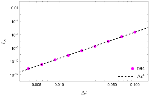
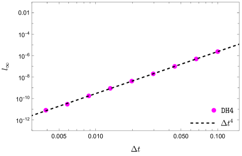
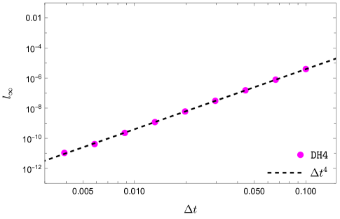
Figure 17: Numerical error associated with computation of the numerical weak-form solution $\Psi(t,x_{f})$ against the exact solution in Eq.(16) (plots on top) and Eq.(15) (plots on bottom) with both the discontinuous IMP implicit and IMTEX implicit-turned-explicit Hermite integrator order-4. Left: The two plots on the left give the implementation of DiscoIMP with an Hermite order-4 scheme as described by the evolution algorithm in Eq.(368). Right: The two plots on the right give the implementation of DiscoTEX with an Hermite order-4 scheme as described by the evolution algorithm in Eq.(133).

C.6 Numerical weak-form solution to wave equations of Type II and III via DiscoTEX and DiscoIMP

To further complement our results in Section 3.4 one gives the solution to wave-like problems of Type II and Type III. Additionally, one will consider the implicit Hermite integration scheme, here called DiscoIMP at fourth-order and compare with DiscoTEX. In previous work, [52] have given an implementation of Type II equations with an implicit Hermite order-2 scheme and using radiation boundary conditions with $v=1/3$, $N=110$ Chebyshev collocation nodes and $J=30$ jumps. One finds these computational factors and those in [80, 81] to not be optimal, particularly the factors in [52] just amount to extra computational cost with no accuracy improvements. The presentation follows very closely to that in Section 3.4 and the terms that follow when not defined here, are as defined in that section. The final evolution algorithm describing DiscoIMP is,

$$\Pi^{n+1}=\Pi^{n}+\textbf{MF}\cdot\bigg{[}\textbf{MR}\cdot\Pi^{n}+\Delta t\textbf{L1}\cdot\Psi^{n}$$

$$+\bigg{(}\frac{\Delta t\textbf{L1}}{2}-\frac{\Delta t^{2}}{12}\textbf{L1}\cdot\textbf{L2}\bigg{)}\cdot\textbf{MA}\cdot\bigg{(}\frac{\Delta t^{2}}{12}(s^{n}-s^{n+1})-\textbf{MA}\cdot\big{(}\Upsilon_{\Pi}$$

$$+\texttt{JH4}_{L2}(\Delta t_{\times},\Delta t)\Xi\bigg{)}+\frac{\Delta t^{2}}{12}\bigg{(}s^{n}-s^{n+1}\bigg{)}+\frac{\Delta t}{2}\bigg{(}s^{n}+s^{n+1}\bigg{)}$$

$$+\frac{\Delta t^{2}}{12}\bigg{(}st^{n}+st^{n+1}\bigg{)}+\Upsilon_{\Psi}+\texttt{JH4}_{L1}(\Delta t_{\times},\Delta t)\Xi\bigg{)}\bigg{]},$$

$$\Psi^{n+1}=\Psi^{n}+\textbf{MA}\cdot\bigg{[}\bigg{(}\frac{\Delta t}{2}\textbf{I}+\frac{\Delta t^{2}}{12}\textbf{L2}\bigg{)}\cdot\bigg{(}\Pi^{n}-\Pi^{n+1}\bigg{)}$$

$$+\frac{\Delta t^{2}}{12}\big{(}s^{n}-s^{n+1}\big{)}+\Upsilon_{\Psi}+\texttt{JH4}_{L2}(\Delta t_{\times},\Delta t)\Xi\bigg{]},$$ (368)

where the matrices $\textbf{MF},\textbf{MR},\textbf{MA}$ are given as,

$$\textbf{MF}=\bigg{[}\textbf{I}-\frac{\Delta t}{2}\textbf{L2}+\frac{\Delta t^{2}}{12}\bigg{(}\textbf{L1}+\textbf{L2}\cdot\textbf{L2}\bigg{)}-\bigg{(}\frac{\Delta t}{2}\textbf{L1}$$

$$-\frac{\Delta t^{2}}{12}\textbf{L1}\cdot\textbf{L2}\bigg{)}\cdot\textbf{MA}\cdot\bigg{(}\frac{\Delta t}{2}\textbf{I}-\frac{\Delta t^{2}}{12}\textbf{L2}\bigg{)}\bigg{]},$$ (369)

$$\textbf{MR}=\bigg{[}\textbf{I}+\frac{\Delta t}{2}\textbf{L2}+\frac{\Delta t^{2}}{12}\bigg{(}\textbf{L1}+\textbf{L2}\cdot\textbf{L2}\bigg{)}+\bigg{(}\frac{\Delta t}{2}\textbf{L1}$$

$$-\frac{\Delta t^{2}}{12}\textbf{L1}\cdot\textbf{L2}\bigg{)}\cdot\textbf{MA}\cdot\bigg{(}\frac{\Delta t}{2}\textbf{I}-\frac{\Delta t^{2}}{12}\textbf{L2}\bigg{)}\bigg{]}$$ (370)

$$\textbf{MA}=\bigg{[}\textbf{I}+\frac{\Delta t^{2}}{12}\textbf{L1}\bigg{]}.$$ (371)

Additionally, here the terms $\texttt{JH4}_{L1/L2}(\Delta t_{\times},\Delta t)$ refer to the time jumps associated with the operators in Eq.(121). As one can see from Fig.(17) the implementation of the algorithm with an implicit IMP scheme Hermite order-4 DiscoIMP and with an IMTEX Hermite order-4 integrator as DiscoTEX retrieves the same accuracy while retaining the same conservation geometric proprieties. In both our simulations the exact same numerical optimisation factors were used with $J=20$ jumps, $N=34$ Chebyshev nodes and a time-step of $\Delta t\approx 0.003$ in a computational domain of $x\in[-6,6]$ and $t\in[-1.52,6.60]$ time-interval. One has decided to use DiscoTEX due to its reduced-form easing computational implementations and because it reduces computational running time.

Appendix D Black hole perturbation theory machinery

Note, unlike in [49], the formalism of [23] is now followed along with their conventions for the spherical harmonic decomposition formalism implementation.

D.1 Projections of the stress-energy tensor

As applied in [23] one uses the decomposition of Martel and Poisson [70],

$$p_{ab}(x^{\mu})=\sum_{l,m}h^{lm}_{ab}Y^{lm}_{B},\ \ \ p_{aB}(x^{\mu})=\sum_{l,m}h^{lm}_{a}Y^{lm}_{B},$$ (372)

$$p_{AB}(x^{\mu})=r^{2}\sum_{l,m}\bigg{(}K^{lm}\Omega_{AB}Y^{lm}+G^{lm}\Omega_{AB}Y^{lm}_{AB}\bigg{)},$$ (373)

where the tensor $\Omega_{AB}$ is the metric on the unit 2-sphere given as,

$$ds^{2}=\Omega_{AB}dx^{A}dx^{B}=d\theta^{2}+\sin^{2}\theta\ d\varphi^{2}.$$ (374)

D.1.1 Polar/ZM projections of the stress-energy tensor

The source terms are given by the even-parity field equations described by Eqs.(C3) in [23].

$$Q^{ab}(t,r)=8\pi\int T^{ab}Y^{*}d\Omega,$$ (375)

$$Q^{a}(t,r)=\frac{16\pi}{l(l+1)}\int T^{aB}Y^{*}_{B}d\Omega,$$ (376)

$$Q^{\flat}(t,r)=8\pi r^{2}\int T^{AB}\Omega_{AB}Y^{*}d\Omega,$$ (377)

$$Q^{\sharp}(t,r)=32\pi r^{4}\frac{(l-2)!}{(l+2)!}\int T^{AB}Y^{*}_{AB}d\Omega.\hskip 56.9055pt$$ (378)

Re-writing this in terms of time-dependent functions,

$$Q^{ab}(t,r)=q^{ab}(t)\delta(r-r_{p}),\ \ \ \ \ Q^{a}(t,r)=q^{a}(t)\delta(r-r_{p}),$$ (379)

$$Q^{\flat}(t,r)=q^{\flat}(t)\delta(r-r_{p}),\ \ \ \ \ Q^{\sharp}(t,r)=q^{\sharp}(t)\delta(r-r_{p}).$$ (380)

The magnitudes of the $q$ terms are given as,

$$q^{tt}(t)=8\pi\mu\frac{\mathcal{E}}{r^{2}_{p}f_{p}}Y^{*},\ \ \ \ q^{rr}(t)=8\pi\mu\frac{f_{p}}{\mathcal{E}r^{2}_{p}}(\mathcal{E}^{2}-U^{2})Y^{*},\ \ \ \$$ (381)

$$q^{tr}(t)=8\pi\mu\frac{u^{r}}{r^{2}_{p}},$$ (382)

$$q^{t}(t)=8\pi\mu\frac{\mathcal{L}}{r^{2}_{p}}Y^{*}_{\varphi},\ \ \ \ q^{r}(t)=\frac{16\pi\mu}{l(l+1)}\frac{\mathcal{L}}{\mathcal{E}}\frac{f_{p}}{r^{2}_{p}}u^{r}Y^{*}_{\varphi},$$ (383)

$$q^{\flat}(t)=8\pi\mu\frac{\mathcal{L}^{2}}{\mathcal{E}}\frac{f_{p}}{r^{4}_{p}}Y^{*},\ \ \ \ q^{\sharp}(t)=32\pi\mu\frac{(l-2)!}{(l+2)!}\frac{\mathcal{L}^{2}}{\mathcal{E}}\frac{f_{p}}{r^{2}_{p}}u^{r}Y^{*}_{\varphi\varphi},$$ (384)

where the spherical harmonics are given as defined in Ref.[23].

D.1.2 Axial/CPM projections of the stress-energy tensor

For the axial perturbations, one has [23, 70],

$$P^{a}(t,r)=\frac{16\pi r^{2}}{l(l+1)}\int T^{aB}X^{*}_{B}d\Omega,$$ (385)

$$P(t,r)=16\pi r^{4}\frac{(l-2)!}{(l+2)!}\int T^{AB}X^{*}_{AB}d\Omega,$$ (386)

as in D.1.1, re-written it as time-dependent functions,

$$P^{a}(t,r) = p^{a}(t)\delta(r-r_{p}),$$ (387)

$$P(t,r) = p(t)\delta(r-r_{p}),$$ (388)

where the magnitude of p is given by,

$$p^{t}(t)=\frac{16\pi\mu}{l(l+1)}\frac{\mathcal{L}}{r^{2}_{p}}X^{*}_{\varphi},\ \ \ p^{r}(t)=\frac{16\pi\mu}{l(l+1)}\frac{\mathcal{L}}{\mathcal{E}}\frac{f_{p}}{r^{2}_{p}}u^{r}X^{*}_{\varphi},$$

$$p(t)=16\pi\mu\frac{(l-2)!}{(l+2)!}\frac{\mathcal{L}}{\mathcal{E}}\frac{f_{p}}{r^{2}_{p}}X^{*}_{\varphi\varphi}.\hskip 56.9055pt$$ (389)

D.2 Axial/CPM source term

The axial/CPM source term describing the perturbations of $\Psi^{a}_{lm}(t,r)$ given in Eq.(200) is,

$$S_{lm}^{a}(t,r_{p}(t))=\bar{F}^{a}_{lm}(t)\delta^{\prime}(r-r_{p}(t))+\bar{G}^{a}_{lm}(t)\delta(r-r_{p}(t)).\ \ \ \$$ (390)

Following the notation of [23] we have,

$$\bar{G}_{lm}^{a}(t) = \mathcal{G}^{r_{1}}_{l}p^{r}_{lm}+\mathcal{G}^{r_{2}}_{l}\frac{dp^{r}_{lm}}{dt}+\mathcal{G}^{t}_{l}p^{t}_{lm},$$ (391)

$$\bar{F}_{lm}^{a}(t) = \mathcal{F}^{r}_{l}p^{r}_{lm}+\mathcal{F}^{t}_{l}q^{t}_{lm},$$ (392)

where,

$$\mathcal{G}_{l}^{r_{1}}(t) = \frac{\dot{r}_{p}}{\lambda},\ \ \ \ \mathcal{G}_{l}^{r_{2}}(t)=\frac{r_{p}}{\lambda},\ \ \ \ \mathcal{G}_{l}^{t}(t)=-\frac{f_{p}}{\lambda},$$ (393)

$$\mathcal{F}_{l}^{r}(t) = -\frac{r_{p}\dot{r}_{p}}{\lambda},\ \ \ \ \mathcal{F}_{l}^{t}(t)=\frac{r_{p}f^{2}_{p}}{\lambda}.$$ (394)

D.3 ZM/Polar source term

The polar/ZM source term describing the perturbations of $\Psi^{p}_{lm}(t,r)$ given in Eq.(200) is,

$$S_{lm}^{p}(t,r_{p}(t))=\bar{F}^{p}_{lm}(t)\delta^{\prime}(r-r_{p}(t))+\bar{G}^{p}_{lm}(t)\delta(r-r_{p}(t)).\ \ \ \$$ (395)

Following the notation of [23] we have,

$$\bar{G}_{lm}^{p}(t)=\mathcal{G}^{rr}_{l}q^{rr}_{lm}+\mathcal{G}^{tt}_{l}q^{tt}_{lm}+\mathcal{G}^{r}_{l}q^{r}_{lm}+\mathcal{G}^{\flat}_{l}q^{\flat}_{lm}+\mathcal{G}^{\sharp}_{l}q^{\sharp}_{lm},$$ (396)

$$\bar{F}_{lm}^{p}(t)=\mathcal{F}^{rr}_{l}q^{rr}_{lm}+\mathcal{F}^{tt}_{l}q^{tt}_{lm},$$ (397)

where,

$$\mathcal{G}_{l}^{rr}(t)=\frac{1}{(\lambda+1)r_{p}\Lambda^{2}_{p}}\bigg{[}(\lambda+1)(\lambda r_{p}+6M)r_{p}+3M^{2}\bigg{]},$$ (398)

$$\mathcal{G}_{l}^{tt}(t)=\frac{f_{p}^{2}}{(\lambda+1)r_{p}\Lambda^{2}_{p}}\bigg{[}\lambda(\lambda+1)r_{p}^{2}+6\lambda Mr_{p}+15M^{2}\bigg{]},$$ (399)

$$\mathcal{G}_{l}^{r}(t)=\frac{2f_{p}}{\Lambda_{p}},\ \ \ \ \mathcal{G}_{l}^{\flat}(t)=\frac{r_{p}f_{p}^{2}}{(\lambda+1)\Lambda_{p}},\ \ \ \mathcal{G}_{l}^{\sharp}(t)=-\frac{f_{p}}{r_{p}},$$ (400)

$$\mathcal{F}_{l}^{rr}(t)=-\frac{r^{2}_{p}f_{p}}{(\lambda+1)\Lambda_{p}},\ \ \ \ \mathcal{F}_{l}^{tt}(t)=-\frac{r^{2}_{p}f_{p}^{3}}{(\lambda+1)\Lambda_{p}}.$$ (401)

References

• [1] X. Huang, H. Liu, B. Shi, Z. Wang, K. Yang, Y. Li, B. Weng, M. Wang, H. Chu, J. Zhou, et al., Solving partial differential equations with point source based on physics-informed neural networks, arXiv preprint arXiv:2111.01394 (2021).
• [2] A. Lipton, V. Kaushansky, C. Reisinger, Semi-analytical solution of a mckean–vlasov equation with feedback through hitting a boundary, European Journal of Applied Mathematics 32 (6) (2021) 1035–1068.
• [3] T. J. Lewis, J. Rinzel, Dynamics of spiking neurons connected by both inhibitory and electrical coupling, Journal of computational neuroscience 14 (2003) 283–309.
• [4] M. J. Cáceres, J. A. Carrillo, B. Perthame, Analysis of nonlinear noisy integrate & fire neuron models: blow-up and steady states, The Journal of Mathematical Neuroscience 1 (1) (2011) 1–33.
• [5] J. A. Carrillo, B. Perthame, D. Salort, D. Smets, Qualitative properties of solutions for the noisy integrate and fire model in computational neuroscience, Nonlinearity 28 (9) (2015) 3365.
• [6] M. J. Cáceres, R. Schneider, Towards a realistic nnlif model: analysis and numerical solver for excitatory-inhibitory networks with delay and refractory periods, arXiv preprint arXiv:1705.02205 (2017).
• [7] L. R. Johnson, Green’s function for lamb’s problem, Geophysical Journal International 37 (1) (1974) 99–131.
• [8] D. Komatitsch, J. Tromp, Introduction to the spectral element method for three-dimensional seismic wave propagation, Geophysical journal international 139 (3) (1999) 806–822.
• [9] M. Dumbser, F. Fambri, M. Tavelli, M. Bader, T. Weinzierl, Efficient implementation of ader discontinuous galerkin schemes for a scalable hyperbolic pde engine, Axioms 7 (3) (2018) 63.
• [10] A. Dembo, L.-C. Tsai, Criticality of a randomly-driven front, Archive for Rational Mechanics and Analysis 233 (2019) 643–699.
• [11] C. Cuchiero, S. Rigger, S. Svaluto-Ferro, Propagation of minimality in the supercooled stefan problem, The Annals of Applied Probability 33 (2) (2023) 1588–1618.
• [12] L. Barack, Gravitational self-force in extreme mass-ratio inspirals, Classical and Quantum Gravity 26 (21) (2009) 213001.
• [13] E. Poisson, A. Pound, I. Vega, The motion of point particles in curved spacetime, Living Reviews in Relativity 14 (2011) 1–190.
• [14] B. Wardell, Self-force: computational strategies, Equations of Motion in Relativistic Gravity (2015) 487–522.
• [15] L. Barack, A. Pound, Self-force and radiation reaction in general relativity, Reports on Progress in Physics 82 (1) (2018) 016904.
• [16] A. Pound, B. Wardell, Black hole perturbation theory and gravitational self-force, Handbook of Gravitational Wave Astronomy (2022) 1–119.
• [17] T. Hinderer, E. E. Flanagan, Two-timescale analysis of extreme mass ratio inspirals in kerr spacetime: Orbital motion, Physical Review D 78 (6) (2008) 064028.
• [18] N. Afshordi, S. Akçay, P. A. Seoane, A. Antonelli, J. C. Aurrekoetxea, L. Barack, E. Barausse, R. Benkel, L. Bernard, S. Bernuzzi, et al., Waveform modelling for the laser interferometer space antenna, arXiv preprint arXiv:2311.01300 (2023).
• [19] J. E. Thompson, H. Chen, B. F. Whiting, Gauge invariant perturbations of the schwarzschild spacetime, Classical and Quantum Gravity 34 (17) (2017) 174001.
• [20] J. E. Thompson, B. Wardell, B. F. Whiting, Gravitational self-force regularization in the regge-wheeler and easy gauges, Physical Review D 99 (12) (2019) 124046.
• [21] T. Regge, J. A. Wheeler, Stability of a schwarzschild singularity, Physical Review 108 (4) (1957) 1063.
• [22] F. J. Zerilli, Gravitational field of a particle falling in a schwarzschild geometry analyzed in tensor harmonics, Physical Review D 2 (10) (1970) 2141.
• [23] S. Hopper, C. R. Evans, Gravitational perturbations and metric reconstruction: Method of extended homogeneous solutions applied to eccentric orbits on a schwarzschild black hole, Physical Review D 82 (8) (2010) 084010.
• [24] S. A. Teukolsky, Rotating black holes: Separable wave equations for gravitational and electromagnetic perturbations, Physical Review Letters 29 (16) (1972) 1114.
• [25] S. A. Teukolsky, Perturbations of a rotating black hole. i. fundamental equations for gravitational, electromagnetic, and neutrino-field perturbations, Astrophysical Journal, Vol. 185, pp. 635-648 (1973) 185 (1973) 635–648.
• [26] W. H. Press, S. A. Teukolsky, Perturbations of a rotating black hole. ii. dynamical stability of the kerr metric, Astrophysical Journal, Vol. 185, pp. 649-674 (1973) 185 (1973) 649–674.
• [27] S. A. Teukolsky, W. H. Press, Perturbations of a rotating black hole. iii-interaction of the hole with gravitational and electromagnetic radiation, Astrophysical Journal, vol. 193, Oct. 15, 1974, pt. 1, p. 443-461. 193 (1974) 443–461.
• [28] S. E. Field, J. S. Hesthaven, S. R. Lau, Discontinuous galerkin method for computing gravitational waveforms from extreme mass ratio binaries, Classical and Quantum Gravity 26 (16) (2009) 165010.
• [29] J. E. Thompson, Functional form of gauge invariants in Rw and Eazy gauges, unpublished work (2018).
• [30] T. Müller, F. Grave, Geodesicviewer–a tool for exploring geodesics in the theory of relativity, Computer Physics Communications 181 (2) (2010) 413–419.
• [31] F. H. Vincent, T. Paumard, E. Gourgoulhon, G. Perrin, Gyoto: a new general relativistic ray-tracing code, Classical and Quantum Gravity 28 (22) (2011) 225011.
• [32] M. Bauböck, D. Psaltis, F. Özel, T. Johannsen, A ray-tracing algorithm for spinning compact object spacetimes with arbitrary quadrupole moments. ii. neutron stars, The Astrophysical Journal 753 (2) (2012) 175.
• [33] D. Psaltis, T. Johannsen, A ray-tracing algorithm for spinning compact object spacetimes with arbitrary quadrupole moments. i. quasi-kerr black holes, The Astrophysical Journal 745 (1) (2011) 1.
• [34] C.-k. Chan, L. Medeiros, F. Özel, D. Psaltis, Gray2: A general purpose geodesic integrator for kerr spacetimes, The Astrophysical Journal 867 (1) (2018) 59.
• [35] C. W. Gear, Numerical initial value problems in ordinary differential equations, Prentice-Hall series in automatic computation (1971).
• [36] O. Kopáček, V. Karas, J. Kovář, Z. Stuchlík, Transition from regular to chaotic circulation in magnetized coronae near compact objects, The Astrophysical Journal 722 (2) (2010) 1240.
• [37] J. Seyrich, G. Lukes-Gerakopoulos, Symmetric integrator for nonintegrable hamiltonian relativistic systems, Physical Review D 86 (12) (2012) 124013.
• [38] U. M. Ascher, S. J. Ruuth, B. T. Wetton, Implicit-explicit methods for time-dependent partial differential equations, SIAM Journal on Numerical Analysis 32 (3) (1995) 797–823.
• [39] U. M. Ascher, S. J. Ruuth, R. J. Spiteri, Implicit-explicit runge-kutta methods for time-dependent partial differential equations, Applied Numerical Mathematics 25 (2-3) (1997) 151–167.
• [40] D. Tsang, C. R. Galley, L. C. Stein, A. Turner, “slimplectic” integrators: variational integrators for general nonconservative systems, The Astrophysical Journal Letters 809 (1) (2015) L9.
• [41] C. Lubich, B. Walther, B. Bruegmann, Symplectic integration of post-newtonian equations of motion with spin, Physical Review D 81 (10) (2010) 104025.
• [42] S.-Y. Zhong, X. Wu, S.-Q. Liu, X.-F. Deng, Global symplectic structure-preserving integrators for spinning compact binaries, Physical Review D 82 (12) (2010) 124040.
• [43] L. Mei, M. Ju, X. Wu, S. Liu, Dynamics of spin effects of compact binaries, Monthly Notices of the Royal Astronomical Society 435 (3) (2013) 2246–2255.
• [44] J. Crank, P. Nicolson, A practical method for numerical evaluation of solutions of partial differential equations of the heat-conduction type, in: Mathematical proceedings of the Cambridge philosophical society, Vol. 43, Cambridge University Press, 1947, pp. 50–67.
• [45] S. A. Teukolsky, Stability of the iterated crank-nicholson method in numerical relativity, Physical Review D 61 (8) (2000) 087501.
• [46] L. J. Gomes Da Silva, “Conformal” discontinuous collocations methods for self-force calculations in the time domain, https://drive.google.com/drive/folders/13XF8tqVCpg1ofioz0CT4HhCX5BPfsc0e (2022).
• [47] L. J. Gomes Da Silva, Numerical algorithms for the modelling of EMRIs in the time domain, PhD dissertation, QMUL University, School of Mathematical Sciences (2023).
• [48] M. F. O’Boyle, C. Markakis, L. J. G. Da Silva, R. P. Macedo, J. A. V. Kroon, Conservative evolution of black hole perturbations with time-symmetric numerical methods, arXiv preprint arXiv:2210.02550 (2022).
• [49] L. J. Gomes Da Silva, R. P. Macedo, J. E. Thompson, J. A. V. Kroon, L. Durkan, O. Long, Hyperboloidal discontinuous time-symmetric numerical algorithm with higher order jumps for gravitational self-force computations in the time domain, arXiv preprint arXiv:2306.13153 (2023).
• [50] R. P. Macedo, M. Ansorg, Axisymmetric fully spectral code for hyperbolic equations, Journal of Computational Physics 276 (2014) 357–379.
• [51] R. Panosso Macedo, L. Gomes Da Silva, et al, Hyperboloidal numerical algorithm for the computation of the scalar self-force on a charged particle on a schwarzschild background in the time domain, in preparation (2024).
• [52] C. Markakis, M. F. O’Boyle, P. D. Brubeck, L. Barack, Discontinuous collocation methods and gravitational self-force applications, arXiv e-prints (2014) arXiv:1406.4865arXiv:1406.4865, doi:10.48550/arXiv.1406.4865.
• [53] L. J. Gomes Da Silva, Numerical algorithms for the modelling of emris in the time domain, PhD first, second and third year reviews, QMUL University, School of Mathematical Sciences (2019-2022).
• [54] L. J. Gomes Da Silva, “Conformal” discontinuous collocations methods for self-force calculations in the time domain, www.caprameeting.org/capra-meetings/capra-24, 2021.
• [55] W. H. Press, S. A. Teukolsky, W. T. Vetterling, B. P. Flannery, Numerical recipes in c++, The art of scientific computing 2 (2007) 1002.
• [56] E. Hairer, C. Lubich, G. Wanner, Geometric Numerical Integration: Structure-Preserving Algorithms for Ordinary Differential Equations, Springer Series in Computational Mathematics, Springer Berlin Heidelberg, 2010.
URL https://books.google.co.uk/books?id=ssrFQQAACAAJ
• [57] L. J. Gomes Da Silva, M. F. O’Boyle, C. Markakis, Symmetry, symplecticity and stability of iterated crank-nicholson, to appear in L.J Gomes Da Silva PhD thesis [47], preliminary results presented at Capra 25th and available for consultation on slides 9-10 at https://drive.google.com/drive/folders/13XF8tqVCpg1ofioz0CT4HhCX5BPfsc0e (2022).
• [58] J. D. Brown, Midpoint rule as a variational-symplectic integrator: Hamiltonian systems, Physical Review D 73 (2) (2006) 024001.
• [59] R. Penrose, Asymptotic properties of fields and space-times, Physical Review Letters 10 (2) (1963) 66.
• [60] H. Friedrich, Cauchy problems for the conformal vacuum field equations in general relativity, Communications in Mathematical Physics 91 (1983) 445–472.
• [61] A. Zenginoğlu, Hyperboloidal foliations and scri-fixing, Classical and Quantum Gravity 25 (14) (2008) 145002.
• [62] A. Zenginoğlu, D. Nunez, S. Husa, Gravitational perturbations of schwarzschild spacetime at null infinity and the hyperboloidal initial value problem, Classical and Quantum Gravity 26 (3) (2009) 035009.
• [63] M. Ansorg, R. P. Macedo, Spectral decomposition of black-hole perturbations on hyperboloidal slices, Physical Review D 93 (12) (2016) 124016.
• [64] J. L. Jaramillo, R. P. Macedo, L. Al Sheikh, Pseudospectrum and black hole quasinormal mode instability, Physical Review X 11 (3) (2021) 031003.
• [65] R. P. Macedo, J. L. Jaramillo, M. Ansorg, Hyperboloidal slicing approach to quasinormal mode expansions: The reissner-nordström case, Physical Review D 98 (12) (2018) 124005.
• [66] R. P. Macedo, Hyperboloidal framework for the kerr spacetime, Classical and Quantum Gravity 37 (6) (2020) 065019.
• [67] R. P. Macedo, B. Leather, N. Warburton, B. Wardell, A. Zenginoğlu, Hyperboloidal method for frequency-domain self-force calculations, Physical Review D 105 (10) (2022) 104033.
• [68] S. E. Field, J. S. Hesthaven, S. R. Lau, Persistent junk solutions in time-domain modeling of extreme mass ratio binaries, Physical Review D 81 (12) (2010) 124030.
• [69] S. E. Field, Exact solutions to distributionally sourced wave equations extending [28] Appendix B, unpublished work (2023).
• [70] K. Martel, E. Poisson, Gravitational perturbations of the schwarzschild spacetime: a practical covariant and gauge-invariant formalism, Physical Review D 71 (10) (2005) 104003.
• [71] Black Hole Perturbation Toolkit, (bhptoolkit.org).
• [72] O. Long, L. Barack, Time-domain metric reconstruction for hyperbolic scattering, Physical Review D 104 (2) (2021) 024014.
• [73] D. Dempsey, Wave propagation on black hole spacetimes, Ph.D. thesis, University of Sheffield, School of Mathematics and Statistics (Sheffield), United Kindgom (2017).
• [74] C. Lanczos, Applied analysis prentice hall, New York (1956).
• [75] C. W. Dyche, On multiple point taylor series expansions (1956).
• [76] C. M. Markakis, M. F. O’Boyle, D. Glennon, K. Tran, P. Brubeck, R. Haas, H.-Y. Schive, K. Uryū, Time-symmetry, symplecticity and stability of euler-maclaurin and lanczos-dyche integration, arXiv preprint arXiv:1901.09967 (2019).
• [77] M. Lotkin, A new integrating procedure of high accuracy, Journal of Mathematics and Physics 31 (1-4) (1952) 29–34.
• [78] C. Markakis, S. Bray, A. Zenginoğlu, Symmetric integration of the 1+1 Teukolsky equation on hyperboloidal foliations of Kerr spacetimes (3 2023). arXiv:2303.08153.
• [79] M. O’Boyle, Discontinuous collocation methods and gravitational self-force applications, https://www.youtube.com/watch?v=s8jgI5hEw1Y (2020).
• [80] M. F. O’Boyle, Time-symmetric integration of partial differential equations with applications to black hole physics, Ph.D. thesis, version 1 (2022).
• [81] M. F. O’Boyle, Time-symmetric integration of partial differential equations with applications to black hole physics, Ph.D. thesis (2022).
• [82] M. F. O’Boyle, C. Markakis, Discontinuous collocation and symmetric integration methods for distributionally-sourced hyperboloidal partial differential equations, arXiv preprint arXiv:2308.02385 (2023).
• [83] A. Zenginoğlu, Asymptotics of schwarzschild black hole perturbations, Classical and Quantum Gravity 27 (4) (2010) 045015.
• [84] S. Bernuzzi, A. Nagar, A. Zenginoğlu, Binary black hole coalescence in the large-mass-ratio limit: the hyperboloidal layer method and waveforms at null infinity, Physical Review D 84 (8) (2011) 084026.
• [85] M. Vishal, S. E. Field, K. Rink, S. Gottlieb, G. Khanna, Towards exponentially-convergent simulations of extreme-mass-ratio inspirals: A time-domain solver for the scalar teukolsky equation with singular source terms, arXiv preprint arXiv:2307.01349 (2023).
• [86] L. Gomes Da Silva, R. Panosso Macedo, J. Thompson, et al, Gravitational self-force numerical computation in the regge-wheeler and eazy gauges in the time-domain, in preparation (2024).
• [87] L. Barack, A. Ori, Mode sum regularization approach for the self-force in black hole spacetime, Physical Review D 61 (6) (2000) 061502.
• [88] A. Heffernan, A. Ottewill, B. Wardell, High-order expansions of the Detweiler-Whiting singular field in Schwarzschild spacetime, Phys. Rev. D 86 (2012) 104023. arXiv:1204.0794, doi:10.1103/PhysRevD.86.104023.
• [89] C. T. Cunningham, R. H. Price, V. Moncrief, Radiation from collapsing relativistic stars. i-linearized odd-parity radiation, Astrophysical Journal, Part 1, vol. 224, Sept. 1, 1978, p. 643-667. 224 (1978) 643–667.
• [90] C. T. Cunningham, R. H. Price, V. Moncrief, Radiation from collapsing relativistic stars. ii-linearized even-parity radiation, Astrophysical Journal, Part 1, vol. 230, June 15, 1979, p. 870-892. 230 (1979) 870–892.
• [91] V. Moncrief, Gravitational perturbations of spherically symmetric systems. i. the exterior problem, Annals of Physics 88 (2) (1974) 323–342.
• [92] L. Barack, N. Sago, Gravitational self-force on a particle in circular orbit around a schwarzschild black hole, Physical Review D 75 (6) (2007) 064021.
• [93] S. Detweiler, Consequence of the gravitational self-force for circular orbits of the schwarzschild geometry, Physical Review D 77 (12) (2008) 124026.
• [94] J. E. Thompson, Gravitational self-force in the Regge-wheeler and Eazy gauges, PhD dissertation, University of Florida (2018).
• [95] C. O. Lousto, R. H. Price, Head-on collisions of black holes: the particle limit, Physical Review D 55 (4) (1997) 2124.
• [96] K. Martel, E. Poisson, One-parameter family of time-symmetric initial data for the radial infall of a particle into a schwarzschild black hole, Physical Review D 66 (8) (2002) 084001.
• [97] K. Martel, Gravitational waveforms from a point particle orbiting a schwarzschild black hole, Physical Review D 69 (4) (2004) 044025.
• [98] L. Barack, P. Giudice, Time-domain metric reconstruction for self-force applications, Physical Review D 95 (10) (2017) 104033.
• [99] C. O. Lousto, A time-domain fourth-order-convergent numerical algorithm to integrate black hole perturbations in the extreme-mass-ratio limit, Classical and Quantum Gravity 22 (15) (2005) S543.
• [100] R. Haas, Scalar self-force on eccentric geodesics in schwarzschild spacetime: a time-domain computation, Physical Review D 75 (12) (2007) 124011.
• [101] L. Barack, N. Sago, Gravitational self-force on a particle in eccentric orbit around a schwarzschild black hole, Physical Review D 81 (8) (2010) 084021.
• [102] C. F. Sopuerta, P. Sun, P. Laguna, J. Xu, A toy model for testing finite element methods to simulate extreme-mass-ratio binary systems, Classical and Quantum Gravity 23 (1) (2005) 251.
• [103] C. F. Sopuerta, P. Laguna, Finite element computation of the gravitational radiation emitted by a pointlike object orbiting a nonrotating black hole, Physical Review D 73 (4) (2006) 044028.
• [104] P. Canizares, C. F. Sopuerta, Efficient pseudospectral method for the computation of the self-force on a charged particle: Circular geodesics around a schwarzschild black hole, Physical Review D 79 (8) (2009) 084020.
• [105] P. Canizares, C. F. Sopuerta, An efficient time-domain method to model extreme-mass-ratio inspirals, arXiv preprint arXiv:1009.6073 (2010).
• [106] P. Canizares, C. F. Sopuerta, Modelling extreme-mass-ratio inspirals using pseudospectral methods, arXiv preprint arXiv:1001.4697 (2010).
• [107] P. Canizares, C. F. Sopuerta, J. L. Jaramillo, Pseudospectral collocation methods for the computation of the self-force on a charged particle: Generic orbits around a schwarzschild black hole, Physical Review D 82 (4) (2010) 044023.
• [108] P. Canizares, C. F. Sopuerta, Tuning time-domain pseudospectral computations of the self-force on a charged scalar particle, Classical and Quantum Gravity 28 (13) (2011) 134011.
• [109] P. Canizares, C. F. Sopuerta, Time-domain modelling of extreme-mass-ratio inspirals for the laser interferometer space antenna, in: Journal of Physics: Conference Series, Vol. 314, IOP Publishing, 2011, p. 012075.
• [110] W. Krivan, P. Laguna, P. Papadopoulos, N. Andersson, Dynamics of perturbations of rotating black holes, Physical Review D 56 (6) (1997) 3395.
• [111] E. Barausse, A. Buonanno, S. A. Hughes, G. Khanna, S. O’Sullivan, Y. Pan, Modeling multipolar gravitational-wave emission from small mass-ratio mergers, Physical Review D 85 (2) (2012) 024046.
• [112] P. A. Sundararajan, G. Khanna, S. A. Hughes, Towards adiabatic waveforms for inspiral into kerr black holes: A new model of the source for the time domain perturbation equation, Physical Review D 76 (10) (2007) 104005.
• [113] P. A. Sundararajan, G. Khanna, S. A. Hughes, S. Drasco, Towards adiabatic waveforms for inspiral into kerr black holes. ii. dynamical sources and generic orbits, Physical Review D 78 (2) (2008) 024022.
• [114] A. Taracchini, A. Buonanno, G. Khanna, S. A. Hughes, Small mass plunging into a kerr black hole: Anatomy of the inspiral-merger-ringdown waveforms, Physical Review D 90 (8) (2014) 084025.
• [115] A. Apte, S. A. Hughes, Exciting black hole modes via misaligned coalescences. i. inspiral, transition, and plunge trajectories using a generalized ori-thorne procedure, Physical Review D 100 (8) (2019) 084031.
• [116] H. Lim, G. Khanna, A. Apte, S. A. Hughes, Exciting black hole modes via misaligned coalescences. ii. the mode content of late-time coalescence waveforms, Physical Review D 100 (8) (2019) 084032.
• [117] S. R. Dolan, L. Barack, Self-force via m-mode regularization and 2+ 1 d evolution: Foundations and a scalar-field implementation on schwarzschild spacetime, Physical Review D 83 (2) (2011) 024019.
• [118] S. R. Dolan, L. Barack, B. Wardell, Self-force via m-mode regularization and 2+ 1 d evolution. ii. scalar-field implementation on kerr spacetime, Physical Review D 84 (8) (2011) 084001.
• [119] L. Barack, D. A. Golbourn, N. Sago, m-mode regularization scheme for the self-force in kerr spacetime, Physical Review D 76 (12) (2007) 124036.
• [120] L. Barack, D. A. Golbourn, Scalar-field perturbations from a particle orbiting a black hole using numerical evolution in 2+ 1 dimensions, Physical Review D 76 (4) (2007) 044020.
• [121] S. R. Dolan, L. Durkan, C. Kavanagh, B. Wardell, Metric perturbations of kerr spacetime in lorenz gauge: Circular equatorial orbits, arXiv preprint arXiv:2306.16459 (2023).
• [122] S. R. Dolan, Superradiant instabilities of rotating black holes in the time domain, Physical Review D 87 (12) (2013) 124026.
• [123] R. Lopez-Aleman, G. Khanna, J. Pullin, Perturbative evolution of particle orbits around kerr black holes: time-domain calculation, Classical and Quantum Gravity 20 (14) (2003) 3259.
• [124] G. Khanna, Teukolsky evolution of particle orbits around kerr black holes in the time domain: Elliptic and inclined orbits, Physical Review D 69 (2) (2004) 024016.
• [125] L. M. Burko, G. Khanna, Accurate time-domain gravitational waveforms for extreme-mass-ratio binaries, Europhysics Letters 78 (6) (2007) 60005.
• [126] J. Thornburg, B. Wardell, Scalar self-force for highly eccentric equatorial orbits in kerr spacetime, Physical Review D 95 (8) (2017) 084043.
• [127] S. Boscarino, Error analysis of imex runge–kutta methods derived from differential-algebraic systems, SIAM Journal on Numerical Analysis 45 (4) (2007) 1600–1621.
• [128] S. Boscarino, On an accurate third order implicit-explicit runge–kutta method for stiff problems, Applied Numerical Mathematics 59 (7) (2009) 1515–1528.
• [129] S. Boscarino, G. Russo, On a class of uniformly accurate imex runge–kutta schemes and applications to hyperbolic systems with relaxation, SIAM Journal on Scientific Computing 31 (3) (2009) 1926–1945.
• [130] A. Nagar, T. Damour, A. Tartaglia, Binary black hole merger in the extreme-mass-ratio limit, Classical and Quantum Gravity 24 (12) (2007) S109.
• [131] T. Damour, A. Nagar, Final spin of a coalescing black-hole binary: An effective-one-body approach, Physical Review D 76 (4) (2007) 044003.
• [132] T. Damour, A. Nagar, Faithful effective-one-body waveforms of small-mass-ratio coalescing black hole binaries, Physical Review D 76 (6) (2007) 064028.
• [133] T. Damour, A. Nagar, Binary black hole merger waveforms in the extreme mass ratio limit, in: The Eleventh Marcel Grossmann Meeting: On Recent Developments in Theoretical and Experimental General Relativity, Gravitation and Relativistic Field Theories (In 3 Volumes), World Scientific, 2008, pp. 1636–1638.
• [134] S. Bernuzzi, A. Nagar, Binary black hole merger in the extreme-mass-ratio limit: a multipolar analysis, Physical Review D 81 (8) (2010) 084056.
• [135] E. Harms, S. Bernuzzi, B. Brügmann, Numerical solution of the 2+ 1 teukolsky equation on a hyperboloidal and horizon penetrating foliation of kerr and application to late-time decays, Classical and Quantum Gravity 30 (11) (2013) 115013.
• [136] E. Harms, S. Bernuzzi, A. Nagar, A. Zenginoğlu, A new gravitational wave generation algorithm for particle perturbations of the kerr spacetime, Classical and Quantum Gravity 31 (24) (2014) 245004.
• [137] S. Albanesi, S. Bernuzzi, T. Damour, A. Nagar, A. Placidi, Faithful effective-one-body waveform of small-mass-ratio coalescing black hole binaries: the eccentric, nonspinning, case, arXiv preprint arXiv:2305.19336 (2023).
• [138] E. Harms, G. Lukes-Gerakopoulos, S. Bernuzzi, A. Nagar, Asymptotic gravitational wave fluxes from a spinning particle in circular equatorial orbits around a rotating black hole, Physical Review D 93 (4) (2016) 044015.
• [139] E. Harms, G. Lukes-Gerakopoulos, S. Bernuzzi, A. Nagar, Spinning test body orbiting around a schwarzschild black hole: Circular dynamics and gravitational-wave fluxes, Physical Review D 94 (10) (2016) 104010.
• [140] E. Schnetter, P. Diener, E. N. Dorband, M. Tiglio, A multi-block infrastructure for three-dimensional time-dependent numerical relativity, Classical and Quantum Gravity 23 (16) (2006) S553.
• [141] I. Vega, B. Wardell, P. Diener, S. Cupp, R. Haas, Scalar self-force for eccentric orbits around a schwarzschild black hole, Physical Review D 88 (8) (2013) 084021.
• [142] P. Diener, E. N. Dorband, E. Schnetter, M. Tiglio, New, efficient, and accurate high order derivative and dissipation operators satisfying summation by parts, and applications in three-dimensional multi-block evolutions, arXiv preprint gr-qc/0512001 (2005).
• [143] Samuel Cupp - Self-consistent time domain evolution using the self-force 1D code framework, The Capra 25th Meeting on Radiation Reaction, https://drive.google.com/drive/folders/13XF8tqVCpg1ofioz0CT4HhCX5BPfsc0e/, accessed: 2023-05-03.
• [144] S. Cupp, From equal-mass to extreme-mass-ratio binary inspirals: Simulation tools for next generation gravitational wave detectors, PhD dissertation, Lousiana State University (2022).
• [145] A. Pound, B. Wardell, N. Warburton, J. Miller, Second-order self-force calculation of gravitational binding energy in compact binaries, Physical review letters 124 (2) (2020) 021101.
• [146] N. Warburton, A. Pound, B. Wardell, J. Miller, L. Durkan, Gravitational-wave energy flux for compact binaries through second order in the mass ratio, Physical Review Letters 127 (15) (2021) 151102.
• [147] B. Wardell, A. Pound, N. Warburton, J. Miller, L. Durkan, A. Le Tiec, Gravitational waveforms for compact binaries from second-order self-force theory, Physical Review Letters 130 (24) (2023) 241402.
• [148] P. Diener, I. Vega, B. Wardell, S. Detweiler, Self-consistent orbital evolution of a particle around a schwarzschild black hole, Physical Review Letters 108 (19) (2012) 191102.
• [149] Capra Community, Capra meetings archive, https://www.caprameeting.org/capra-meetings (2024).
• [150] A. Sekhar, Subrahmanyan Chandrasekhar: A man of stellar physics and stellar grace, https://thewire.in/the-sciences/subrahmanyan-chandrasekhar-a-man-of-stellar-physics-and-stellar-grace, accessed: 31/10/2023.
• [151] E. W. Weisstein, Frobenius method, https://mathworld. wolfram. com/ (2002).
• [152] G. Frobenius, Ueber die integration der linearen differentialgleichungen durch reihen (1873).
• [153] P. D. Brubeck, Jump Relations in PDEs, Unpublished notes.
• [154] J. Mathews, A. Pound, B. Wardell, Self-force calculations with a spinning secondary, Physical Review D 105 (8) (2022) 084031.
• [155] X.-N. Su, X. Wu, F.-Y. Liu, Application of the logarithmic hamiltonian algorithm to the circular restricted three-body problem with some post-newtonian terms, Astrophysics and Space Science 361 (2016) 1–12.
• [156] S. Hu, X. Wu, E. Liang, An energy-conserving integrator for conservative hamiltonian systems with ten-dimensional phase space, The Astrophysical Journal Supplement Series 253 (2) (2021) 55.