We construct a set of parton distribution functions (PDFs), based on the recent NNPDF4.0 PDF set, that also include a photon PDF. The photon PDF is constructed using the LuxQED formalism, while QED evolution accounting for $\mathcal{O}\left(\alpha\right)$, $\mathcal{O}\left(\alpha\alpha_{s}\right)$, and $\mathcal{O}\left(\alpha^{2}\right)$ corrections is implemented and benchmarked by means of the EKO code. We investigate the impact of QED effects on NNPDF4.0, and compare our results both to our previous NNPDF3.1QED PDF set and to other recent PDF sets that include the photon. We assess the impact of photon-initiated processes and electroweak corrections on a variety of representative LHC processes, and find that they can reach the 5% level in vector boson pair production at large invariant mass.

1 Introduction

High precision physics at the LHC, especially in its high-luminosity era [1, 2, 3], will demand the inclusion of electroweak corrections in the computation of theoretical predictions for hard processes [4]. This requires an extension of the set of proton parton distribution functions (PDFs). In particular a photon PDF has to be provided, and evolution equations need to be supplemented with QED splitting functions. The photon PDF enables the inclusion of photon-initiated processes, which typically are enhanced in the high-mass and large transverse-momentum tails of the distributions. In principle, at high-enough scales, proton PDFs should also include PDFs for leptons [5], gauge bosons [6] and indeed for the full set of 52 standard model fields [7], or even new hypothetical particles such as dark photons [8]. However, in practice, the main requirement of current precision physics at the LHC is the availability of PDF sets that also include a photon PDF, that mixes upon combined QED$\times$QCD evolution with the standard quark and gluon PDFs. We will henceforth refer to such PDF sets as “QED PDFs”.

Initial attempts at the construction of QED PDF sets relied on models for the photon PDF at the initial evolution scale [9, 10]. A first data-driven determination of QED PDFs, based on a fit using the NNPDF2.3 methodology [11, 12], resulted in a photon PDF with large uncertainties. The fact that determining the photon PDF from the data yields a result affected by large uncertainties was more recently confirmed in determinations based on fitting to the data PDFs with a fixed functional forms within the xFitter methodology [13] applied to high-mass ATLAS Drell–Yan distributions [14].

A breakthrough in the determination of QED PDFs was achieved in 2016 in Refs. [15, 16] (see also related results in Refs. [17, 18]), where it was shown that the photon PDF can be computed perturbatively in QED, given as input the proton structure functions at all scales, from the elastic ($Q^{2}\to 0$) to the deep-inelastic ($Q^{2}\to\infty$) regimes — the so-called LuxQED method. Since then, this LuxQED framework has been the basis of all QED PDF sets [19, 20, 21, 22, 23].

While the effect of the inclusion of the photon PDF on other PDFs is small, it is not negligible within current uncertainties. For instance, the photon typically carries a fraction of the proton momentum which is about two orders of magnitude smaller than that of the gluon, so the corresponding depletion of the gluon momentum fraction is relevant at the percent level, which is comparable to the size of the current uncertainty on the gluon PDF. Precision calculations of LHC processes with electroweak effects thus require a consistent global QED PDF determination.

With this motivation, we construct a QED PDF set based on the recent NNPDF4.0 PDF determination [24, 25], including QED corrections to parton evolution up to $\mathcal{O}\left(\alpha\alpha_{s}\right)$ and $\mathcal{O}\left(\alpha^{2}\right)$. We follow closely the methodology developed for the NNPDF3.1QED PDFs in Ref. [19], based on an iterative procedure. Namely, we evaluate the photon PDF at some fixed scale using the LuxQED formula and the structure function computed from an existing PDF set, now NNPDF4.0. We evolve it together with the other PDFs to the initial parametrization scale $Q_{0}=1.65$ GeV. We then re-determine the quark and gluon PDFs while also including this photon PDF as a boundary condition to the QCD$\times$QED evolution. We compute the photon PDF again using LuxQED, and we iterate until convergence.

All results presented in this paper are obtained using a new theory implementation, now adopted by default in the NNPDF public code [25]. In particular, the APFEL [26] and APFELgrid [27] codes have been replaced by a suite of newly developed tools including the evolution equations solver EKO [28], the DIS structure functions calculator YADISM [29], and the interpolator of hard-scattering cross-sections PineAPPL [30, 31]. Taken together, they provide a pipeline for the efficient automatization of the computation of theory predictions [32]. An integral component of this theory pipeline is the use of interpolation grids in the format provided by PineAPPL [30, 31], which can be interfaced to Monte Carlo generators. Among these is mg5_aMC@NLO [33], which automates NLO QCD+EW calculations for a wide range of LHC processes where knowledge of QED PDFs is crucial.

The outline of this paper is as follows. First, Sect. 2 reviews the theoretical framework underlying the NNPDF4.0QED determination and in particular the implementation of QED evolution in EKO. Then the NNPDF4.0QED PDFs are presented in Sect. 3, where they are compared to the previous NNPDF3.1QED PDF set, and to other recent QED PDF sets. Implications for LHC phenomenology are studied in Sect. 4 by means of the PineAPPL interface to mg5_aMC@NLO. Conclusions and an outline of future developments are finally presented in Sect. 5. Because this paper is, as mentioned, the first to make use of a new theory pipeline, and specifically its implementation of combined QCD$\times$QED evolution, a set of benchmarks is collected in two appendices. Specifically, in Appendix A we benchmark NNPDF4.0 PDFs determined using the old and new pipeline and show that they are indistinguishable; in Appendix B the new implementation of joint QCD and QED evolution of PDFs in the EKO code is discussed and benchmarked against the previous implementation in the APFEL code.

2 Evolution and determination of QED PDFs

In this section, we discuss the structure of combined QED$\times$QCD evolution and we briefly review the methodology used to determine QED PDFs. This methodology is based on the LuxQED formalism [15, 16], and was developed for the construction of the NNPDF3.1QED PDF set [19].

2.1 QCD$\times$QED evolution equations and basis choice

The scale dependence of PDFs is determined by evolution equations of the form

$$\mu^{2}\frac{df_{i}(N,\mu^{2})}{d\mu^{2}}=-\sum_{j}\gamma_{ij}\left(N,a_{s}(\mu^{2}),a_{em}(\mu^{2})\right)f_{j}(N,\mu^{2})\,,$$ (2.1)

where $f_{i}(N,\mu^{2})=\int_{0}^{1}dx\,x^{N-1}f_{i}(x,\mu^{2})$ is the Mellin transform of the $i$-th PDF. The anomalous dimensions $\gamma_{ij}(N,a_{s},a_{em})$ are determined as a simultaneous perturbative expansion in the strong coupling $a_{s}=\alpha_{s}/(4\pi)$ and in the electromagnetic coupling $a_{em}=\alpha/(4\pi)$:

$$\gamma_{ij}(N,a_{s},a_{em}) =\sum_{\begin{subarray}{c}n,m=0\\ (n,m)\neq(0,0)\end{subarray}}^{\infty}a_{s}^{n}a_{em}^{m}\gamma_{ij}^{(n,m)}(N)$$ (2.2)

$$=a_{s}\gamma_{ij}^{(1,0)}(N)+a_{s}^{2}\gamma_{ij}^{(2,0)}(N)+a_{s}^{3}\gamma_{ij}^{(3,0)}(N)$$

$$\hskip 10.0pt+a_{em}\gamma_{ij}^{(0,1)}(N)+a_{em}^{2}\gamma_{ij}^{(0,2)}(N)+a_{s}a_{em}\gamma_{ij}^{(1,1)}(N)+\dots\,.$$

In this work we include pure QCD corrections up to NNLO, $\gamma^{(1,0)}$, $\gamma^{(2,0)}$, and $\gamma^{(3,0)}$ [34, 35]; the pure NLO QED corrections $\gamma^{(0,1)}$ and $\gamma^{(0,2)}$ [36]; and the leading mixed correction $\gamma^{(1,1)}$ [37].

The scale dependence of the strong and electromagnetic couplings is in turn determined by coupled renormalization group equations of the form

$$\mu^{2}\frac{da_{s}}{d\mu^{2}} =\beta_{{}_{\rm QCD}}(a_{s},a_{em})=-a_{s}^{2}\left(\beta_{{}_{\rm QCD}}^{(2,0)}+a_{s}\beta_{{}_{\rm QCD}}^{(3,0)}+a_{em}\beta_{{}_{\rm QCD}}^{(2,1)}+a_{s}^{2}\beta_{{}_{\rm QCD}}^{(4,0)}\dots\right)\,,$$ (2.3)

$$\mu^{2}\frac{da_{em}}{d\mu^{2}} =\beta_{{}_{\rm QED}}(a_{s},a_{em})=-a_{em}^{2}\left(\beta_{{}_{\rm QED}}^{(0,2)}+a_{em}\beta_{{}_{\rm QED}}^{(0,3)}+a_{s}\beta_{{}_{\rm QED}}^{(1,2)}+\dots\right)\,,$$ (2.4)

in terms of the coefficients of the corresponding QCD and QED beta functions. Consistently with the treatment of evolution equations, we include pure QCD contributions up to NNLO, namely $\beta_{{}_{\rm QCD}}^{(2,0)}$, $\beta_{{}_{\rm QCD}}^{(3,0)}$, and $\beta_{{}_{\rm QCD}}^{(4,0)}$; pure QED up to NLO, namely $\beta_{{}_{\rm QED}}^{(0,2)}$ and $\beta_{{}_{\rm QED}}^{(0,3)}$; and the leading mixed terms $\beta_{{}_{\rm QCD}}^{(2,1)}$ and $\beta_{{}_{\rm QED}}^{(1,2)}$ [38]. We adopt the $\overline{\rm{MS}}$ scheme. Schemes in which the electroweak coupling does not run, such as the $G_{\mu}$ scheme, are commonly used in the computation of electroweak corrections, but $\overline{\rm{MS}}$ is more convenient when considering combined QCD and QED corrections [39, 40]. Equations (2.1–2.4) must then be simultaneously solved with a common scale $\mu$.

The solution is most efficiently obtained in a maximally decoupled basis in quark flavor space. This requires adopting a suitable combination of quark and antiquark flavors such that the sum over $j$ in Eq. (2.1) contains the smallest possible number of entries. In the case of QCD-only evolution, this is achieved in the so-called evolution basis, in which one separates off the singlet combination $\Sigma=\sum_{i}(q_{i}+\bar{q}_{i})$, which mixes with the gluon, and then one constructs nonsinglet combinations of individual C-even (sea-like) and C-odd (valence-like) $q^{\pm}_{i}=q_{i}\pm\bar{q}_{i}$ quark and antiquark flavors, each of which evolves independently.

Because the photon couples differently to up-like $u_{k}=\{u,c,t\}$ and down-like $d_{k}=\{d,s,b\}$ quarks, a different basis choice is necessary when also including QED. To this end, given $n_{f}$ active quark flavors, we split them into $n_{u}$ up-like and $n_{d}$ down-like flavors, such that $n_{f}=n_{u}+n_{d}$, and define the four combinations

$$\Sigma_{u}=\sum_{k=1}^{n_{u}}u_{k}^{+},\quad\Sigma_{d}=\sum_{k=1}^{n_{d}}d_{k}^{+},\quad V_{u}=\sum_{k=1}^{n_{u}}u_{k}^{-},\quad V_{d}=\sum_{k=1}^{n_{d}}d_{k}^{-}.$$ (2.5)

Also, we separate off the QCD contributions to the anomalous dimensions, by rewriting the perturbative expansion of the anomalous dimensions, Eq. 2.2, as

$$\gamma_{ij}(N,a_{s},a_{em})=\gamma_{ij}(N,a_{s})+\tilde{\gamma}_{ij}(N,a_{s},a_{em})\,,$$ (2.6)

where $\gamma_{ij}(a_{s})$ contains the pure QCD contributions and $\tilde{\gamma}_{ij}$ contains both the pure QED and the mixed QCD$\times$QED corrections.

The maximally decoupled evolution equations are then constructed as follows. The nonsinglet combinations

$$T_{3}^{d} =d^{+}-s^{+}\,, V_{3}^{d} =d^{-}-s^{-}\,, T_{3}^{u} =u^{+}-c^{+}\,, V_{3}^{u} =u^{-}-c^{-}\,,$$ (2.7)

$$T_{8}^{d} =d^{+}+s^{+}-2b^{+}\,, V_{8}^{d} =d^{-}+s^{-}-2b^{-}\,, T_{8}^{u} =u^{+}+c^{+}-2t^{+}\,, V_{8}^{u} =u^{-}+c^{-}-2t^{-}\,,$$ (2.8)

evolve independently according to nonsinglet evolution equations of the form

$$\mu^{2}\frac{d}{d\mu^{2}}T^{u/d}_{3/8} =-(\gamma_{\rm ns,+}+\tilde{\gamma}^{\rm ns,+}_{u/d})T^{u/d}_{3/8}\,,$$ (2.9)

$$\mu^{2}\frac{d}{d\mu^{2}}V^{u/d}_{3/8} =-(\gamma_{\rm ns,-}+\tilde{\gamma}^{\rm ns,-}_{u/d})V^{u/d}_{3/8}\,.$$ (2.10)

The valence sum and difference combinations, defined as

$$V=V_{u}+V_{d}\,,\quad V_{\Delta}=\frac{n_{d}}{n_{u}}V_{u}-V_{d}\,,$$ (2.11)

satisfy coupled evolution equations

$$\mu^{2}\frac{d}{d\mu^{2}}\begin{pmatrix}V\\ V_{\Delta}\end{pmatrix}=-\begin{pmatrix}\gamma^{{\rm ns},V}+\langle\tilde{\gamma}^{{\rm ns},-}_{q}\rangle&\nu_{u}\tilde{\gamma}^{{\rm ns},-}_{\Delta q}\\ \nu_{d}\tilde{\gamma}^{{\rm ns},-}_{\Delta q}&\gamma^{{\rm ns},-}+\{\tilde{\gamma}^{{\rm ns},-}_{q}\}\end{pmatrix}\begin{pmatrix}V\\ V_{\Delta}\end{pmatrix}\,,$$ (2.12)

in terms of the linear combinations of anomalous dimensions

$$\nu_{u/d}=\frac{n_{u/d}}{n_{f}}\,,\quad\langle\tilde{\gamma}^{{\rm ns},\pm}_{q}\rangle=\nu_{u}\tilde{\gamma}^{{\rm ns},\pm}_{u}+\nu_{d}\tilde{\gamma}^{{\rm ns},\pm}_{d}\,,\quad\{\tilde{\gamma}^{{\rm ns},\pm}_{q}\}=\nu_{d}\tilde{\gamma}^{{\rm ns},\pm}_{u}+\nu_{u}\tilde{\gamma}^{{\rm ns},\pm}_{d}\,,\quad\tilde{\gamma}^{{\rm ns},\pm}_{\Delta q}=\tilde{\gamma}^{{\rm ns},\pm}_{u}-\tilde{\gamma}^{{\rm ns},\pm}_{d}\,.$$ (2.13)

Finally, the gluon and photon satisfy coupled evolution equations together with the quark singlet sum and difference combinations, defined as

$$\Sigma=\Sigma_{u}+\Sigma_{d},\quad\Sigma_{\Delta}=\frac{n_{d}}{n_{u}}\Sigma_{u}-\Sigma_{d}\,.$$ (2.14)

These coupled evolution equations read

$$\mu^{2}\frac{d}{d\mu^{2}}\begin{pmatrix}g\\ \gamma\\ \Sigma\\ \Sigma_{\Delta}\end{pmatrix}=-{\mathbf{\Gamma}}\begin{pmatrix}g\\ \gamma\\ \Sigma\\ \Sigma_{\Delta}\end{pmatrix}\,,$$ (2.15)

with ${\mathbf{\Gamma}}$ a $4\times 4$ anomalous dimension matrix of the form

$${\mathbf{\Gamma}}=\begin{pmatrix}\gamma_{gg}+\tilde{\gamma}_{gg}&\tilde{\gamma}_{g\gamma}&\gamma_{gq}+\langle\tilde{\gamma}_{gq}\rangle&\nu_{u}\tilde{\gamma}_{g\Delta q}\\ \tilde{\gamma}_{\gamma g}&\tilde{\gamma}_{\gamma\gamma}&\langle\tilde{\gamma}_{\gamma q}\rangle&\nu_{u}\tilde{\gamma}_{\gamma\Delta q}\\ 2n_{f}(\gamma_{qg}+\langle\tilde{\gamma}_{qg}\rangle)&2n_{f}\langle\tilde{\gamma}_{q\gamma}\rangle&\gamma_{qq}+\langle\tilde{\gamma}^{{\rm ns},+}_{q}\rangle+\langle e^{2}_{q}\rangle^{2}\tilde{\gamma}_{{\rm ps}}&\nu_{u}\tilde{\gamma}^{{\rm ns},+}_{\Delta q}+\nu_{u}e^{2}_{\Delta q}\langle e^{2}_{q}\rangle\tilde{\gamma}_{{\rm ps}}\\ 2n_{f}\nu_{d}\tilde{\gamma}_{\Delta qg}&2n_{f}\nu_{d}\tilde{\gamma}_{\Delta q\gamma}&\nu_{d}\tilde{\gamma}^{{\rm ns},+}_{\Delta q}+\nu_{d}e^{2}_{\Delta q}\langle e^{2}_{q}\rangle\tilde{\gamma}_{{\rm ps}}&\gamma^{{\rm ns},+}+\{\tilde{\gamma}^{{\rm ns},+}_{q}\}+\nu_{u}\nu_{d}(e^{2}_{\Delta q})^{2}\tilde{\gamma}_{{\rm ps}}\end{pmatrix}\,,$$

where $\tilde{\gamma}^{{\rm ps}}_{qq^{\prime}}=e^{2}_{q}e^{2}_{q^{\prime}}\tilde{\gamma}_{{\rm ps}}$ [36], and the combinations $\langle\tilde{\gamma}_{gq}\rangle$, $\langle\tilde{\gamma}_{qg}\rangle$, $\tilde{\gamma}_{g\Delta q}$, $\tilde{\gamma}_{\Delta qg}$, $\langle\tilde{\gamma}_{\gamma q}\rangle$, $\langle\tilde{\gamma}_{q\gamma}\rangle$, $\tilde{\gamma}_{\gamma\Delta q}$, and $\tilde{\gamma}_{\Delta q\gamma}$ are constructed analogously to those listed in Eq. (2.13).

The basis defined by Eqs. 2.7, 2.8, 2.11 and 2.14 is denoted as the unified evolution basis. Compared to the basis used in APFEL [26] to solve the QCD$\times$QED evolution equations, our definitions of $\Sigma_{\Delta}$ and $V_{\Delta}$ differ due to the prefactors $n_{d}/n_{u}$ that make the basis fully orthogonal. In the presence of scale-independent intrinsic heavy quarks (e.g. a charm-quark PDF in a three-flavor scheme [41]), a further decomposition needs to be applied [28].

The unified flavor basis has been implemented in the EKO code [28], which, as discussed in the introduction, is now used to solve evolution equations as part of the new theory pipeline. The basic ingredient of the EKO code is the construction of evolution kernel operators $E(Q^{2}\leftarrow Q_{0}^{2})$ (EKOs) such that

$$f(Q^{2})=E(Q^{2}\leftarrow Q_{0}^{2})f(Q_{0}^{2}),$$ (2.16)

where $f(Q^{2})$ is a vector whose components are all PDF flavors, including all active quark and antiquark flavors in a suitable basis, the photon and the gluon. Formally, the EKOs are given by

$$E(Q^{2}\leftarrow Q_{0}^{2})=\mathcal{P}\exp\left(-\int_{Q_{0}^{2}}^{Q^{2}}\frac{{\rm d}\mu^{2}}{\mu^{2}}\,\gamma\left(a_{s}(\mu^{2}),a_{em}(\mu^{2})\right)\right)\,,$$ (2.17)

where $\gamma$ is the full matrix of anomalous dimensions, and $\mathcal{P}$ denotes path ordering. In the unified evolution basis the evolution kernel is a block diagonal matrix, with individual diagonal entries for the nonsinglet combinations Eqs. (2.7,2.8) (without path-ordering), a $2\times 2$ block for the valence combinations Eq. (2.11), and a $4\times 4$ block in the singlet sector.

A variety of implementations of the solution of the evolution equations, each of those corresponding to a determination of the EKO, and which differ by higher-order terms, are available in the EKO code. These are discussed in Ref. [28]. At NNLO in QCD, the solutions are essentially indistinguishable in the data region. The solution adopted here is the iterated-exact (EXA) of Ref. [28], while the truncated (TRN) solution was adopted for the NNPDF3.1QED [19] and NNPDF4.0 [24] PDF sets, using the APFEL [26] implementation. These different implementations (at NNLO) are benchmarked and shown to be equivalent in Appendix B, where we also discuss the motivations for this choice.

2.2 Construction of the photon PDF

As mentioned in Sect. 1, the photon PDF is determined using the LuxQED [15, 16] formalism, implemented in a PDF fit using the same methodology as the one used for the NNPDF3.1QED PDF set [19], but now with the new theory pipeline. The LuxQED result amounts to proving that the photon PDF is perturbatively determined in QED by knowledge of the proton inclusive structure functions $F_{2}$ and $F_{L}$:

$$\begin{split}&x\gamma(x,\mu^{2})=\frac{2}{a_{em}(\mu^{2})}\int\limits_{x}^{1}\frac{dz}{z}\Biggl{\{}\int_{m_{p}^{2}x^{2}\over(1-z)}^{\mu^{2}\over(1-z)}\frac{dQ^{2}}{Q^{2}}a_{em}^{2}(Q^{2})\Biggl{[}-z^{2}F_{L}(x/z,Q^{2})\\ &+\left(zP_{\gamma q}(z)+\frac{2x^{2}m_{p}^{2}}{Q^{2}}\right)F_{2}(x/z,Q^{2})\Biggr{]}-a_{em}^{2}(\mu^{2})z^{2}F_{2}(x/z,\mu^{2})\Biggr{\}}\,,\end{split}$$ (2.18)

where $m_{p}$ is the mass of the proton and $P_{\gamma q}$ is the photon-quark splitting function. Equation (2.18) holds in the $\overline{\rm MS}$ scheme, including terms of order $a_{em}$ and $a_{em}^{2}\ln\mu^{2}/m_{p}^{2}$, times the accuracy of the QCD determination of the structure functions.

The integration over the scale $Q^{2}$ and Bjorken-$x$ dependence of the structure functions $F_{i}(x,Q^{2})$ in Eq. (2.18) includes four different regions and corresponding contributions to the structure functions: an elastic contribution at $x=1$, a resonance contribution when $x$ is large and close to $x=1$, an inelastic non-perturbative contribution at low $Q^{2}$ and intermediate $x$ and an inelastic perturbative region for intermediate $x$ and large $Q^{2}$. The first three contributions must be determined by fits to lepton-proton scattering data, but the latter contribution may be determined by expressing the structure functions through perturbative QCD factorization in terms of quark and gluon PDFs. In a global PDF determination, one may choose to determine the photon PDF using the LuxQED formula Eq. (2.18) at a single chosen scale $\mu^{2}=Q_{\gamma}^{2}$, and then evolve jointly the photon and all other PDFs through the QCD$\times$QED evolution equations discussed in Sect. 2.1. An alternative option is to determine the photon PDF using Eq. (2.18) at all scales. The two choices are equivalent because the LuxQED photon Eq. (2.18) satisfies the joint QED$\times$QCD evolution equations to the accuracy of the LuxQED formula itself, though they differ by higher-order corrections and also due to the fact that the LuxQED photon is partly determined from a parametrization of data. The former choice was made for the construction of our previous NNPDF3.1QED set [19], which we follow here, also in the choice of parametrization of the structure functions in the non-perturbative region. The same choice was made in Refs. [19, 20, 21, 22, 23], though in Refs. [22, 23] a PDF set in which the photon PDF is determined using Eq. (2.18) at all scales was also presented.

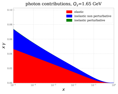
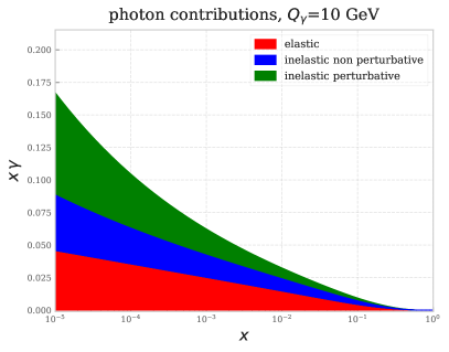
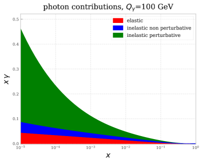
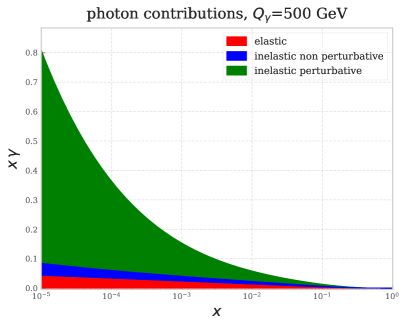
Figure 2.1: Breakdown of the photon PDF $\gamma(x,\mu^{2})$ into the contributions coming from different contributions to the proton structure functions $F_{i}(x,Q^{2})$ that determine it according to the LuxQED formula Eq. (2.18). The result is shown as a function of $x$ for four different choices of the scale $\mu=Q_{\gamma}$: $Q_{\gamma}=1.65$ GeV (top left), 10 GeV (top right), 100 GeV (bottom left) and 500 GeV (bottom right).

The relative size of the elastic, inelastic non-perturbative (including resonances) and elastic perturbative contributions to $\gamma(x,\mu^{2})$ is displayed in Fig. 2.1 as a function of $x$ for four different choices of the scale $\mu=Q_{\gamma}$ at which the LuxQED formula Eq. (2.18) is used to determine the photon. If the LuxQED formula is used at the scale $Q_{\gamma}=1.65$ GeV at which the NNPDF4.0 PDFs are parametrized, the photon is entirely determined by the elastic and non-perturbative contributions, but as the scale is increased, an increasingly large contribution comes from the perturbative region. By the time a value $Q_{\gamma}\gtrsim 100$ GeV is reached, the photon is almost entirely determined by the perturbative contribution, except at very small $x$. Choosing a large value of $Q_{\gamma}$ has the dual advantage that the LuxQED result is more accurate at high scale, because it includes contributions of order $a_{em}$ and $a_{em}^{2}\ln\mu^{2}/m_{p}^{2}$, and also that one is then mostly relying on the accurate perturbative determination of the structure functions, that exploits global information on quarks and gluon PDFs and not just the lepton-proton scattering data. As in Ref. [19], we choose $\mu=Q_{\gamma}=100$ GeV, as also advocated in Ref. [16]. We will discuss the dependence of our results on the choice of scale $Q_{\gamma}$ in Sect. 3.

Equation (2.18) must be viewed as a constraint on the set of photon, quark and gluon PDFs that are simultaneously determined. Because of the small impact of the photon PDF on the other PDFs, it was suggested in Ref. [19] that the constraint can be implemented iteratively. Namely, we first determine the photon PDF using Eq. (2.18) by means of structure functions that are determined from an existing PDF set at a given scale $\mu=Q_{\gamma}$. This photon PDF is then evolved, by solving joint QCD$\times$ QED evolution equations with the unchanged given set, to a chosen PDF parametrization scale where it is taken as fixed. All other PDFs are then re-determined, with the constraint that the momentum sum rule now also includes a contribution from the given (fixed) photon, i.e.

$$\int_{0}^{1}dx\,\left(x\Sigma(x,Q^{2})+xg(x,Q^{2})+x\gamma(x,Q^{2})\right)=1\,.$$ (2.19)

The photon PDF at a scale $\mu=Q_{\gamma}$ is then determined again from Eq. (2.18), in which structure functions are obtained from the new fit. The procedure is iterated until convergence, which was achieved in two iterations in the NNPDF3.1QED determination [19].

Here we follow the same procedure, starting with a re-determination of the NNPDF4.0 PDF set with the new pipeline, which is compared and shown to be equivalent to the published NNPDF4.0 in Appendix A.

3 The NNPDF4.0QED parton distributions

We present here the NNPDF4.0QED PDFs: we first summarize our procedure, then discuss the effect on fit quality of the inclusion of the photon PDF, examine the photon PDF itself, also in comparison to other determinations, and finally study the photon momentum fraction.

3.1 Construction of the NNPDF4.0QED parton set

As mentioned in Sect. 2 all the methodological aspects and settings of the PDF determination are the same as used for the underlying pure QCD NNPDF4.0 PDF [24], but now using a new theory pipeline. Even if in principle theory predictions should be independent of implementation details, in practice differences may arise, e.g. due to issues of numerical accuracy. Also, in the process of transitioning to this new pipeline, a few minor bugs in data implementation were uncovered and fixed. Finally, the new pipeline includes a new implementation of heavy-quark mass effect in deep-inelastic structure functions that differs by subleading terms from the previous one. Benchmarks showing the equivalence of the old and new pipeline are briefly presented in Appendix A. Because of this equivalence, NNPDF4.0 PDF replicas produced with the new pipeline should be considered equivalent to the published ones, and indeed for phenomenological applications (specifically those presented in Sect. 4) we will compare the results obtained using NNPDF4.0QED PDFs to pure QCD results obtained using the published NNPDF4.0 replicas. Nevertheless, in this section only, for all comparisons between pure QCD and QCD$\times$QED, we will use NNPDF4.0 pure QCD replicas generated using the new pipeline, in order to avoid even small confounding effects. Note however that, as discussed in the end of Sect. 2.1, the QED PDFs are based on the EXA solution of the evolution equations, that differs by subleading terms from the TRN solution used in the pure QCD fit. The effect of this difference is assessed in Appendix B and is very small at NNLO. However, all comparisons between pure QCD and QED PDFs also include the effect of this change.

The NNPDF4.0QED PDFs are determined at NLO and NNLO by supplementing with a photon PDF the pure QCD PDF set, according to the methodology outlined in the previous section. However, all theory predictions are obtained as in the pure QCD determination: hence in particular no photon-induced contributions are included, and thus the only effect of the inclusion of a photon PDF is through its mixing with other PDFs. This is justified because the NNPDF4.0 dataset was constructed including cuts that remove all datapoints for which the effect of electroweak corrections is larger than the experimental uncertainties (see Ref. [24], Sect. 4.1). The inclusion of the electroweak corrections, which will allow relaxing these cuts, is left for future work. As in Ref. [19], the final PDF set is obtained after two iterations, with a third iteration providing a check of convergence.

3.2 Fit quality

Table 3.1 displays the statistical estimators obtained using a set of 100 NNPDF4.0QED NLO and NNLO PDF replicas, compared to their QCD-only counterparts, generated using the new theory pipeline. Specifically, we show the $\chi^{2}$, for both the full dataset and for datasets grouped by process; for the full dataset we also show the average over replicas of the training and validation figures of merit $\left\langle E_{\rm tr}\right\rangle_{\rm rep}$ and $\left\langle E_{\rm val}\right\rangle_{\rm rep}$, and the average $\chi^{2}$ over replicas $\left\langle\chi^{2}\right\rangle_{\rm rep}$, all as defined in Table 9 of Ref. [43]. Note that $\chi^{2}$ and $\left\langle\chi^{2}\right\rangle_{\rm rep}$ are computed using the experimental covariance matrix, while, as in all NNPDF determinations, the figure of merit used for minimization is computed using the $t_{0}$ covariance matrix [44].

	Dataset	NNPDF4.0 NLO		NNPDF4.0 NNLO
		QCD$\times$QED	QCD	QCD$\times$QED	QCD
$\chi^{2}$	Global	1.31	1.26	1.17	1.17
$\left\langle E_{\rm tr}\right\rangle_{\rm rep}$		2.47$\pm$0.07	2.41$\pm$0.06	2.27$\pm$0.06	2.28$\pm$0.05
$\left\langle E_{\rm val}\right\rangle_{\rm rep}$		2.66$\pm$0.11	2.57$\pm$0.10	2.39$\pm$0.10	2.37$\pm$0.11
$\left\langle\chi^{2}\right\rangle_{\rm rep}$		1.337$\pm$0.016	1.286$\pm$0.017	1.192$\pm$0.014	1.195$\pm$0.015
$\chi^{2}$	DIS neutral-current	1.38	1.31	1.22	1.23
	DIS charged-current	0.94	0.92	0.90	0.90
	Drell–Yan (inclusive and with one jet)	1.56	1.56	1.30	1.31
	Top-quark pair production	2.31	1.98	1.31	1.24
	Single-top production	0.38	0.36	0.39	0.36
	Inclusive jet production	0.83	0.85	0.93	0.96
	Dijet production	1.56	1.55	1.94	2.03
	Direct photon production	0.64	0.58	0.74	0.75

Table 3.1: Statistical estimators for NNPDF4.0QED NLO and NNLO, compared to NNPDF4.0 pure QCD. From top to bottom: total $\chi^{2}$ per number of data points, average over replicas of the training and validation figures of merit $\left\langle E_{\rm tr}\right\rangle_{\rm rep}$ and $\left\langle E_{\rm val}\right\rangle_{\rm rep}$, average $\chi^{2}$ over replicas $\left\langle\chi^{2}\right\rangle_{\rm rep}$, $\chi^{2}$ for datasets grouped by process. The total number of data points is 4424 (4616) at NLO (NNLO).

It is clear from Table 3.1 that all estimators corresponding are essentially unchanged by the inclusion of QED corrections, with slightly larger differences seen at NLO than at NLO: the impact of QED effects on fit quality is negligible, both globally and for individual processes. Specifically, the training and validation figures of merit in the pure QCD and QCD$\times$QED determinations differ by less than one sigma. As mentioned, these differences also include the effect of switching from the TRN solution of evolution equations in the pure QCD fit to the EXA solution. The impact of this change is yet smaller than that of the QED corrections, but it slightly reduces it.

3.3 The photon PDF

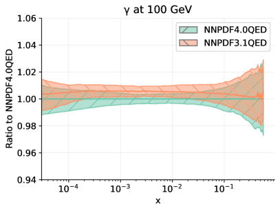
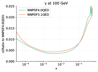
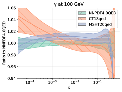
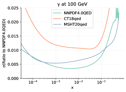
Figure 3.1: Top left: the photon PDF at $Q=100$ GeV in NNPDF4.0QED NNLO compared to its NNPDF3.1QED counterpart as a ratio to the central value of the former. Top right: the relative PDF uncertainties on the photon PDF in these two determinations. Bottom: same as top panels now comparing NNPDF4.0QED with MSHT20QED [21] and CT18QED [22] (all NNLO). Bands correspond to 1$\sigma$ uncertainties.

In Fig. 3.1, the NNLO NNPDF4.0QED photon PDF at $Q=100$ GeV is compared to its counterpart in our previous NNPDF3.1QED [19] set, and in the recent QED PDF sets MSHT20QED [21], and CT18QED [23]. Here and elsewhere in this paper all uncertainties correspond to 1$\sigma$. Results agree at the percent level, despite the fact that quark and gluon PDFs in these sets can display much larger differences. This is a consequence of the fact that in all these PDF sets the photon PDF is determined with the LuxQED formalism in terms of the proton structure function, and that the latter, in turn, is well constrained by experimental data both at high and low scale. In fact, we have checked that the dominant contribution to the difference between the NNPDF3.1QED and NNPDF4.0QED photon PDFs seen in Fig. 3.1 is due to the difference between the TRN and EXA solutions of evolution equations (see Section 3.1 and Appendix B), i.e. to higher-order corrections, with the residual difference being due to the change in the PDFs used in order to compute the structure function. The fact that the 3.1 and 4.0 PDFs are compatible within uncertainties is thus a consequence of the fact that the uncertainties due to higher-order corrections and to PDFs are correctly accounted for by the LuxQED construction, while the NNPDF4.0 PDFs are backward-compatible with the NNPDF3.1 PDFs [24].

The uncertainty on the photon PDF is completely dominated by theoretical uncertainties on the LuxQED procedure, which include [16] missing higher order corrections, uncertainties on the experimentally measured low-scale structure function and so on. In our uncertainty determination we follow Ref. [16]; MSHT also mostly follows this reference, with an extra higher-twist contribution due to the low choice of scale $Q_{\gamma}$, [20] and indeed finds a very similar uncertainty. A somewhat more conservative uncertainty estimate is provided by CT18QED [23], which also adopts a somewhat different determination of the elastic contribution.

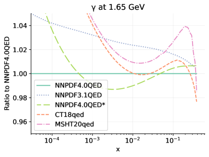
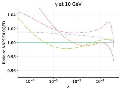
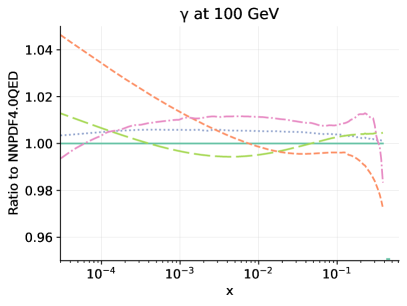
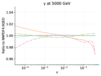
Figure 3.2: Scale dependence of the central photon PDF in the NNPDF4.0QED, NNPDF3.1QED, MSHT20QED, and CT18QED PDF sets. The NNPDF4.0QED result in which the photon is determined at $Q=10$ GeV (denoted as NNPDF4.0QED*) is also shown.

In Fig. 3.2 the central value of the photon PDF in all these sets is compared at different scales, using the native scale dependence of each PDF set. Uncertainties are not shown in order not to clutter the plot. Note that differences in the scale dependence of the PDFs compared in the Figure also arise due to somewhat different treatments of the QCD$\times$QED evolution equations. Specifically, the NNPDF3.1QED PDF set adopts a numerical implementation of the TRN solution (see Appendix B). However, one would expect differences to be mostly driven by the mixing with the quark and gluon PDFs. The fact that differences grow at low scales suggests that this is indeed the case. Even so, all photon PDFs agree within about 3% for all $x\gtrsim 10^{-3}$, even at the lowest scale $Q=1.65$ GeV.

In Fig. 3.2 we also show the central photon PDF which is found by repeating the NNPDF4.0QED determination with the photon PDF determined at a scale $Q_{\gamma}=10$ GeV instead of the default $Q_{\gamma}=100$ GeV. If a low value of $Q_{\gamma}$ is adopted, the upper limit of integration in $Q^{2}$, Eq. 2.18, is accordingly lower. As discussed in Sect. 2.2 in such a case a sizable contribution to the LuxQED formula comes from the low-scale region in which the structure function is determined from a fit to the data, and ${\cal O}\left(\frac{m_{p}}{Q}\right)$ corrections to the LuxQED formula may then become relevant. We see that the shift in central photon PDF which is found by making this choice instead of the default one is at most of the order of the uncertainty on the photon PDF. Again, this shows that the uncertainty on the LuxQED procedure is correctly estimated.

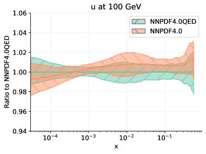
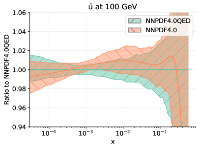
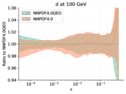
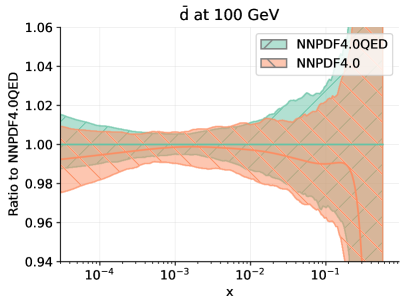
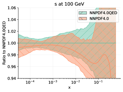
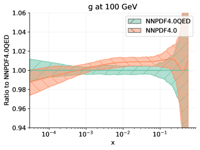
Figure 3.3: Comparison of PDFs in the NNPDF4.0QED and the NNPDF4.0 (pure QCD) sets, shown as a ratio to the former at $Q=100$ GeV. Bands correspond to 1$\sigma$ uncertainties. From left to right and from top to bottom, the up, anti-up, down, anti-down, strange, and gluon PDFs are shown.

We finally assess the impact of the inclusion of a photon PDF on the other PDFs, by comparing the NNLO NNPDF4.0QED and NNPDF4.0 (pure QCD) PDFs. In Fig. 3.3 we present this comparison at $Q=100$ GeV. It is clear that the impact of the inclusion of the photon is moderate, with the NNPDF4.0 (pure QCD) and NNPDF4.0QED PDFs generally differing by less than one sigma and always in agreement within uncertainties. The largest effects are seen in the gluon PDF, which is suppressed at the percent level due to the momentum fraction transferred from the gluon to the photon.

3.4 The photon momentum fraction

The main impact of the photon on other PDFs is through its contribution to the momentum sum rule, Eq. (2.19). We quantify this contribution by evaluating the photon momentum fraction

$$M\left[\gamma(Q)\right]\equiv\int_{0}^{1}dx\,x\gamma(x,Q)\,.$$ (3.1)

In Fig. 3.4 the momentum fractions carried by the photon and by the gluon PDFs in the NNPDF4.0QED set are shown (in percentage) as a function of scale. For the photon the result is compared to that of NNPDF3.1QED, and for the gluon to that of NNPDF4.0 (pure QCD). The photon momentum fraction in the NNPDF3.1QED and NNPDF4.0QED PDF sets is essentially the same: the photon carries around 0.2% of the proton momentum at a low (Q$\sim$1 GeV) scale, growing logarithmically with $Q$ up to around 0.6% at the multi-TeV scale. The momentum fraction carried by the gluon is reduced by a comparable amount upon inclusion of the photon.

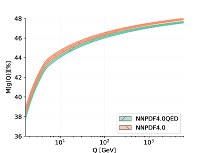
Figure 3.4: Left: the percentage momentum fraction carried by the photon PDF $\gamma(x,Q^{2})$ in NNPDF4.0QED and in NNPDF3.1QED as a function of the scale $Q$, where the bands indicate 1$\sigma$ uncertainties. Right: same for the momentum fraction carried by the gluon PDF in NNPDF4.0QED and in NNPDF4.0 (pure QCD).

4 Implications for LHC phenomenology

We now study the phenomenological implications of the NNPDF4.0QED PDF set. First we compare parton luminosities to those computed using other QED PDF sets. Then we assess the impact of QED corrections on selected processes, by comparing to the pure QCD case calculations that include photon-induced contributions, and also by directly comparing results obtained using NNPDF4.0 (pure QCD) and NNPDF4.0QED PDFs.

4.1 Luminosities

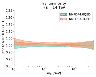
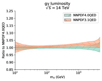
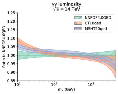
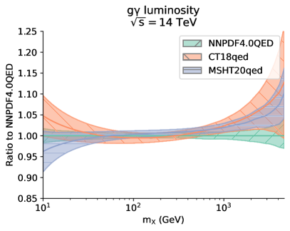
Figure 4.1: The photon-induced contributions to the luminosity at the LHC with $\sqrt{s}=14$ TeV as a function of the invariant mass $m_{X}$ for NNPDF4.0QED NNLO compared to its NNPDF3.1QED counterpart (top) and compared to MSHT20QED and CT18QED, all shown as a ratio to NNPDF4.0QED.

The phenomenological effect on the parton luminosity of the inclusion of a photon PDF is both direct, through the presence of photon-induced partonic channels, and indirect, through the effect of the photon on other PDFs, mostly through the depletion of the gluon that is necessary in order to preserve the momentum sum rule, as discussed in Sect. 3.3-3.4. The photon-induced contributions for NNPDF4.0QED NNLO are compared in Fig. 4.1 to their counterpart in NNPDF3.1QED (top) and in MSHT20QED and CT18QED (bottom). The level of agreement is high and directly follows from that seen between the respective photon PDFs in Figs. 3.1

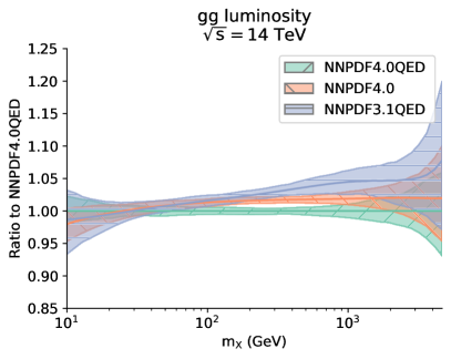
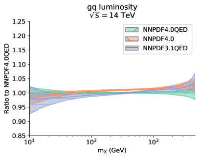
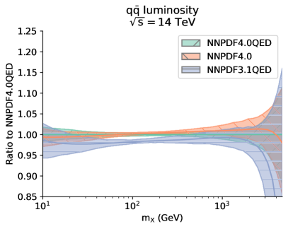
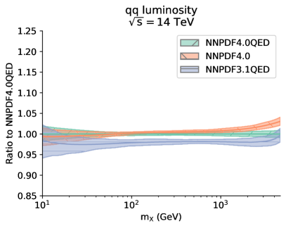
Figure 4.2: Comparison of parton luminosities in the NNPDF4.0QED and the NNPDF4.0 (pure QCD) sets, shown as a ratio to the former for the LHC with $\sqrt{s}=14$ TeV. From left to right and from top to bottom the gluon-gluon, gluon-quark, quark-antiquark and quark-quark luminosities are shown.

The luminosities for all other parton channels are shown in Fig. 4.2, where we compare NNPDF4.0QED both to the previous set NNPDF3.1QED and to the pure QCD NNPDF4.0. Because, as shown in Sect. 3, the effect of the inclusion of the photon on the other PDFs is moderate, the comparison between the two QED sets is very similar to the comparison between the pure QCD NNPDF4.0 and NNPDF3.1 shown in Fig. 9.1 of Ref. [24], where it was shown that NNPDF4.0 are backward compatible, i.e. generally agree with NNPDF3.1 within uncertainties. The effect of the inclusion of QED corrections is, as expected, mostly seen in the gluon–gluon channel, where it leads to a suppression of a few percent in the $m_{X}\sim 100$ GeV region in order to account for the transfer of a small amount of momentum to the photon. The comparison to other PDF sets is dominated by the differences in the quark and gluon PDFs, which are rather more significant than the difference in the photon PDF, and thus very similar to the corresponding comparison of pure QCD luminosities shown in Fig. 9.3 of Ref. [24].

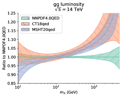
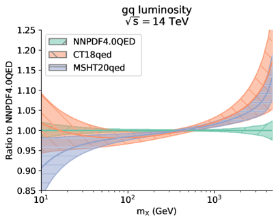
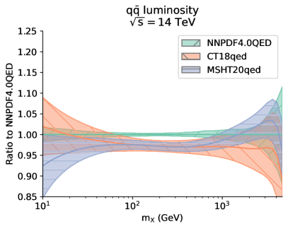
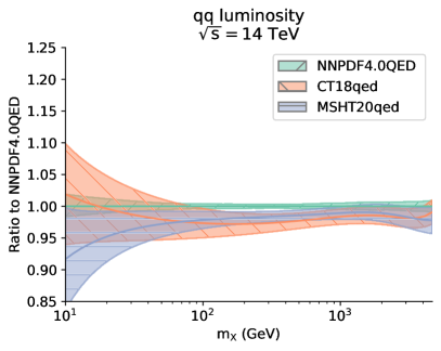
Figure 4.3: Same as Fig. 4.2, now comparing NNPDF4.0QED to MSHT20 [21] and CT18qed [23].

4.2 Physics processes

We now study the impact of the photon PDF on a few representative processes: Drell–Yan production (neutral- and charged-current), Higgs production in gluon-gluon fusion, in vector boson fusion, and in associated production with weak bosons, diboson production, and top-quark pair production, all at the LHC with center-of-mass energy $\sqrt{s}=14$ TeV. We have computed theory predictions for these processes exploiting the PineAPPL [30, 31] interface to the automated QCD and EW calculations provided by mg5_aMC@NLO [33]. PineAPPL produces interpolation grids, accurate to NLO in both the strong and electroweak couplings, that are independent of PDFs. They therefore make it easy to vary the input PDF set, since the same grid can be used for all PDF sets considered. As we are interested in assessing differences between PDF sets, rather than in doing precision phenomenology, we do not include NNLO QCD corrections, and we only show PDF uncertainties. For a detailed list of parameters and cuts used in the calculation of these grids, see Sect. 9 of Ref. [24].

For all processes, we display predictions in figures below with a standardized format, as follows. We show the absolute distributions (top panels) and the ratio to the central value obtained using NNPDF4.0QED PDFs and including photon-induced channels, which we call NNPDF4.0QED (bottom panels). In the left plots we compare NNPDF4.0QED to: NNPDF4.0QED but with no photon-initiated channels; NNPDF4.0 pure QCD; NNPDF3.1QED. In the right plots we compare NNPDF4.0QED to MSHT20QED and CT18QED. The left plots allow for assessing the overall size of the QED corrections (by comparison of the QED and pure QCD results), and disentangling the size of the photon-initiated contributions (by comparison of predictions with the photon-initiated channels switched on and off) and the impact of the changes in the quark and gluon PDFs due to QED effects (by comparison of NNPDF4.0 with NNPDF4.0QED with the photon-initiated channels switched off).

When comparing results obtained using different QED PDF sets, be they NNPDF3.1QED, MSHT20QED or CT18QED, we expect the observed differences to be driven by the change in quark and gluon PDFs, given the similarity of the photon PDF in all sets. Indeed, all comparisons are quite similar to those shown in Sect. 9.3 of Ref. [24], where the same processes were studied in pure QCD.

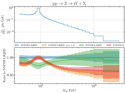
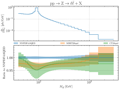
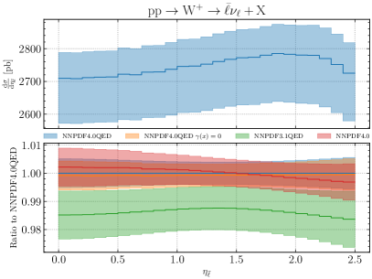
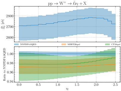
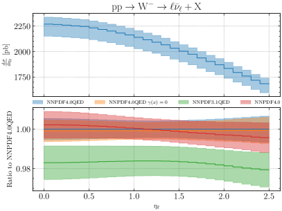
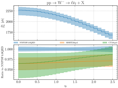
Figure 4.4: Predictions for inclusive Drell–Yan production at the LHC with center-of-mass energy $\sqrt{s}=14$ TeV, computed at NLO accuracy in the QCD and electroweak couplings. All uncertainties shown are PDF uncertainties only. From top to bottom: dilepton production mediated by a $\gamma^{*}/Z$ boson as a function of the dilepton invariant mass $m_{\ell\bar{\ell}}$; $W^{+}$ production as a function of the antilepton pseudo-rapidity $\eta_{\bar{l}}$; $W^{-}$ production as a function of the antilepton pseudo-rapidity $\eta_{l}$. For each process, we display the absolute distributions (top panels) and the ratio to the central value obtained with NNPDF4.0QED PDFs, including photon–initiated channels (bottom panels). In the left panels the full NNPDF4.0 result is compared to NNPDF4.0 (QCD only), NNPDF3.1QED, NNPDF4.0QED (no photon-initiated); in the right panels it is compared to MSHT20QED [21] and CT18QED [23].

In Fig. 4.4 we show results for inclusive Drell–Yan production both in the neutral-current and charged-current channels. For neutral current we show results for the invariant mass distribution of the dilepton pair, while for charged-current we display the rapidity distribution of the lepton. Photon-initiated contributions are most important in the high-mass region, where they reach up to 5%, while they are negligible in the region of the $Z$ peak. This remains true regardless of the particular QED PDF set that is being used. Predictions based on NNPDF4.0QED and NNPDF3.1QED PDFs agree within uncertainties for $m_{\ell\bar{\ell}}\mathrel{\hbox to0.0pt{\lower 4.0pt\hbox{\hskip 1.0pt$\sim$}\hss}\raise 1.0pt\hbox{$>$}}200$ GeV and below the $Z$-peak, $m_{\ell\bar{\ell}}\mathrel{\hbox to0.0pt{\lower 4.0pt\hbox{\hskip 1.0pt$\sim$}\hss}\raise 1.0pt\hbox{$<$}}200$ GeV, with an enhancement of around 2% in the $Z$-peak regions.

Predictions for the Higgs rapidity distribution are shown in Fig. 4.5 for the gluon fusion, associated production with a $W^{+}$ boson, and in vector boson fusion. Finally, in Fig. 4.6 we show predictions for weak-boson pair production ($W^{+}W^{-}$ and $W^{+}Z$), as a function of the dilepton transverse momentum, and for top-quark pair production as a function of the invariant mass of the pair. The impact of photon-initiated contributions is the largest in the $W^{+}W^{-}$ final state, reaching up to 5% for the largest $p_{T,\ell\bar{\ell}}$ values considered. In most cases QED corrections are at the percent level.

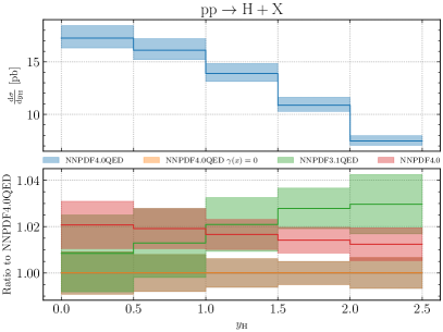
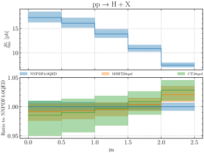
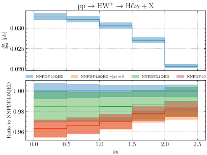
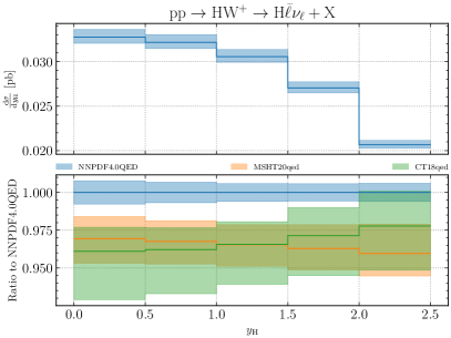
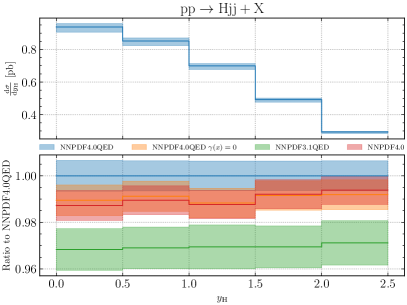
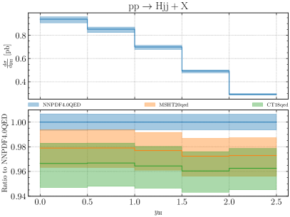
Figure 4.5: Same as Fig. 4.4 but for the rapidity distribution of the Higgs for production in gluon-gluon fusion (top panel), in association with a $W^{+}$ boson (middle panel) and in vector-boson fusion (bottom panel).

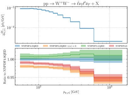
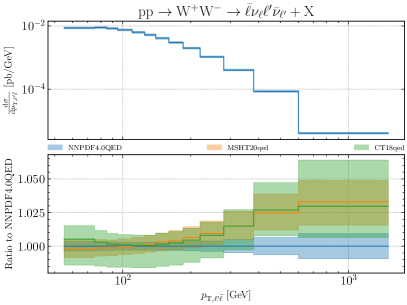
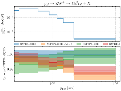
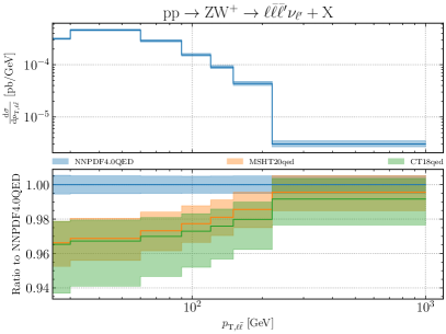
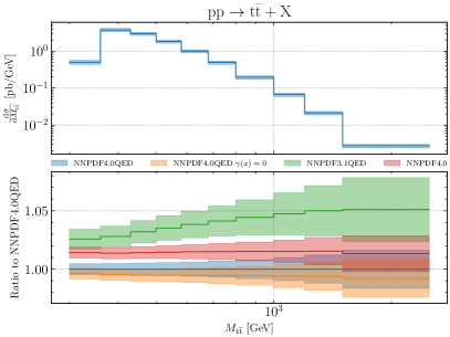
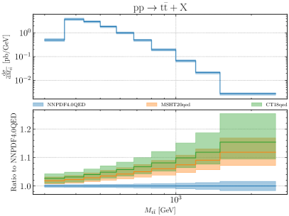
Figure 4.6: Same as Fig. 4.4 but for the dilepton transverse momentum distribution for weak boson pair production ($W^{+}W^{-}$ and $W^{+}Z$) and for the invariant mass distribution for top-quark pair production. No acceptance cuts on the decay productions of the $W,Z$ bosons and top quark have been imposed.

5 Summary and outlook

We have presented a new determination of QED PDFs based on the NNPDF4.0 set of parton distributions, using the methodology previously adopted for the construction of the NNPDF3.1QED PDFs [19]. This methodology implements the LuxQED procedure [15, 16] to determine the photon PDF. Results are consistent with previous studies: specifically, we find that QED effects have a small but non-negligible impact mostly on the gluon PDF, and that photon-initiated contributions are most important for high-mass process such as neutral-current Drell–Yan production. This PDF determination is based on a new NNPDF pipeline for producing theory predictions [32]. Thanks to the integration of QED evolution in this pipeline, and in particular thanks to the use of the EKO evolution code [28], the production of QED variants of NNPDF determinations is now essentially automated, and will become the default in future releases. Indeed, there is in general no reason to switch off the photon PDF, even if it is a small correction, nor to neglect its effect on the momentum fraction carried by the gluon.

The NNPDF4.0QED PDF sets are made publicly available via the LHAPDF6 interface,

http://lhapdf.hepforge.org/  .

All sets are delivered as sets of $N_{\rm rep}=100$ Monte Carlo replicas. Specifically, we provide the NLO and NNLO global fits constructed with the settings defined in Sect. 2 and denoted as

NNPDF40_nlo_as_01180_qed
NNPDF40_nnlo_as_01180_qed

These sets are also made available via the NNPDF collaboration website

https://nnpdf.mi.infn.it/nnpdf4-0-qed/  .

They should be considered the QED PDF counterparts of the published NNPDF4.0 QCD-only PDF sets [24].

We also make available the set of 100 NNPDF4.0 (QCD only) replicas used to produce the comparisons shown in Sect. 3. These differ from the published NNPDF4.0 PDFs because they have been produced using the new theory pipeline, and include some minor bug corrections in the implementation of the NNPDF4.0 dataset. These are called:

NNPDF40_nlo_as_01180_qcd
NNPDF40_nnlo_as_01180_qcd .

The equivalence of these replicas to the published NNPDF4.0 replicas is demonstrated in Appendix A. They are made available for completeness, on the NNPDF website only.

The NNPDF4.0QED determination is part of a family of developments based on the NNPDF4.0 PDF set, and aimed at increasing its accuracy. These will also include a determination of the theory uncertainty on NNPDF4.0 PDFs based on the methodology of Refs. [46, 47], and a first PDF determination based on NNPDF methodology at approximate N³LO [48]. All of these, as well as their combination, will become part of the default NNPDF methodology in future releases.

A natural development of QED PDFs is the full inclusion of electroweak corrections in theory predictions used for PDF determination, which enables a widening of both the set of processes and the kinematic range that may be used for PDF determination, which are currently constrained by the need of ensuring that electroweak corrections are small. This is especially important as electroweak effects become more relevant in regions of phase space sensitive to the large-$x$ PDFs, which are in turn relevant for new physics searches [49, 50]. This development will be greatly facilitated by the availability, within the new pipeline, of the PineAPPL interface to automated Monte Carlo generators, such as mg5_aMC@NLO. All these developments will help achieve PDF determination with percent or sub-percent accuracy.

Acknowledgments

We thank Valerio Bertone for assistance with the benchmarking of QED evolution with APFEL, and Lucian Harland-Lang and Luca Buonocore for discussions on the LuxQED procedure. R. D. B, L. D. D., and R. S. are supported by the U.K. Science and Technology Facility Council (STFC) grant ST/T000600/1. F. H. is supported by the Academy of Finland project 358090 and is funded as a part of the Center of Excellence in Quark Matter of the Academy of Finland, project 346326. E. R. N. is supported by the Italian Ministry of University and Research (MUR) through the “Rita Levi-Montalcini” Program. M. U. and Z. K. are supported by the European Research Council under the European Union’s Horizon 2020 research and innovation Programme (grant agreement n.950246), and partially by the STFC consolidated grant ST/L000385/1. J. R. is partially supported by NWO, the Dutch Research Council. C. S. is supported by the German Research Foundation (DFG) under reference number DE 623/6-2.

Appendix A The new NNPDF theory pipeline

As mentioned in Sect. 3, this work is based on a new pipeline for the calculation of theoretical predictions. This new theory pipeline is described in Ref. [32]; it supersedes and replaces the one used for the NNPDF4.0 determination, which was based on a combination of different pieces of code of various origin, specifically APFEL [26] for PDF evolution and DIS structure function computation, and APFELgrid [27] for the generation of interpolation grids of NLO partonic matrix elements. This last piece of code made use of APPLgrid [51] and FastNLO [52] interpolators. The main benefit of the new pipeline is its unified, yet modular and flexible, structure.

This theory pipeline has been extensively benchmarked for numerical accuracy, including QCD evolution, the computation of structure functions, the interpolation of grids, and the interfacing to mg5_aMC@NLO. Using this new pipeline, interpolation grids for a number of processes have been recomputed, as discussed below. Therefore Tables 2.1–2.5 in Ref. [24] should be updated accordingly.

• All fully inclusive DIS processes (Table 2.1 in Ref. [24]) have been recomputed using YADISM [29, 53]. Specifically, in this code heavy quark mass effects are accounted for using a new implementation of the FONLL prescription [54].

• All fixed-target Drell–Yan processes (see Table 2.3 in Ref. [24]) have been recomputed using a modified version [32] of VRAP [55].

• The following datasets of Table 2.4 and Table 2.5 in Ref. [24] have been recomputed using mg5_aMC@NLO (all grids, in the PineAPPL format, are available at https://github.com/NNPDF/pineapplgrids):

  • ATLAS $W,Z$ 7 TeV ($\mathcal{L}=4.6~{}\text{fb}^{-1}$)

  • ATLAS low-mass DY 7 TeV

  • ATLAS high-mass DY 7 TeV

  • ATLAS $\sigma_{tt}^{\rm tot}$ 7, 8

  • ATLAS $\sigma_{tt}^{\rm tot}$ 13 ($\mathcal{L}=139~{}\text{fb}^{-1}$)

  • ATLAS $t\bar{t}$ lepton+jets 8 TeV

  • ATLAS $t\bar{t}$ dilepton 8 TeV

  • CMS Drell–Yan 2D 7 TeV

  • CMS $t\bar{t}$ 2D dilepton 8 TeV

  • CMS $t\bar{t}$ lepton+jets 13 TeV

  • CMS $t\bar{t}$ dilepton 13 TeV

  • CMS $\sigma_{tt}^{\rm tot}$ 5.02 TeV

  • CMS $\sigma_{tt}^{\rm tot}$ 7, 8 TeV

  • CMS $\sigma_{tt}^{\rm tot}$ 13 TeV

  • LHCb $Z$ 7 TeV ($\mathcal{L}=940~{}\text{pb}^{-1}$)

  • LHCb $Z\to ee$ 8 TeV ($\mathcal{L}=2~{}\text{fb}^{-1}$)

  • LHCb $W,Z\to\mu$ 7 TeV

  • LHCb $W,Z\to\mu$ 8 TeV

Grids for all remaining datasets have been converted to the PineAPPL format without recomputing them. Of course, none of these changes except the new FONLL implementation should make any difference to the extent that the previous and new theory implementations are both numerically accurate. The new FONLL implementation differs from the previous one by subleading corrections and thus it does introduce NNLO differences in the NLO fit and N³LO differences in the NNLO fit; these differences are confined to the charm and bottom mass corrections to deep-inelastic structure functions and thus only affect a small number of datapoints, at NNLO at the sub-percent level.

Finally, in the process of transitioning to the new pipeline, a few bugs were discovered in the implementation of a few datapoints, such as incorrect normalization, incorrect scale assignment or incorrect bin size. These corrections in practice have a negligible impact, as they involve a handful of points out of more than 4500.

	NLO QCD		NNLO QCD
	New	Published	New	Published
$\chi^{2}$	1.26	1.24	1.17	1.16
$\left\langle E_{\rm tr}\right\rangle_{\rm rep}$	2.41 $\pm$ 0.06	2.43 $\pm$ 0.08	2.28 $\pm$ 0.05	2.27 $\pm$ 0.07
$\left\langle E_{\rm val}\right\rangle_{\rm rep}$	2.57 $\pm$ 0.10	2.62 $\pm$ 0.13	2.37 $\pm$ 0.11	2.35 $\pm$ 0.11
$\left\langle\chi^{2}\right\rangle_{\rm rep}$	1.29 $\pm$ 0.02	1.27 $\pm$ 0.02	1.20 $\pm$ 0.02	1.18 $\pm$ 0.02
$\left\langle{\rm TL}\right\rangle_{\rm rep}$	12900 $\pm$ 2000	13200 $\pm$ 2100	12400 $\pm$ 2600	13400 $\pm$ 2400
$\phi$	0.156 $\pm$ 0.006	0.178 $\pm$ 0.007	0.153 $\pm$ 0.005	0.162 $\pm$ 0.005

Table A.1: Statistical indicators (defined as in Table 3.1 for a set of 100 NNPDF4.0 NNLO PDF replicas produced using the new theory pipeline compared to published NNPDF4.0 NNLO 100 replica set. The $\phi$ estimator, defined in Ref. [56], Eq. (4.6), is also shown (see text).

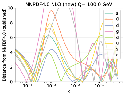
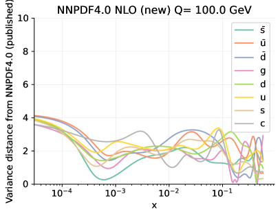
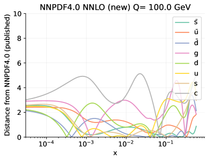
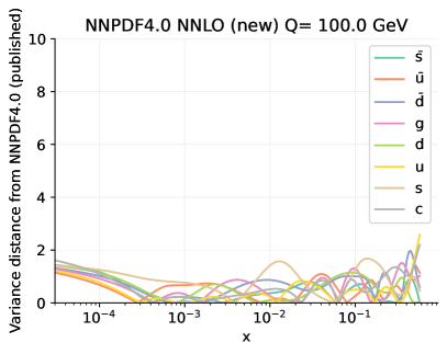
Figure A.1: Distances at $Q=100$ GeV between the central values (left) and uncertainties (right) of the 100 NNPDF4.0 PDF replicas at NLO (top) and NNLO (bottom) whose statistical indicators are compared in Table A.1.

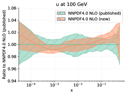
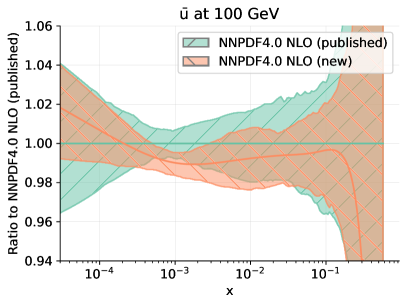
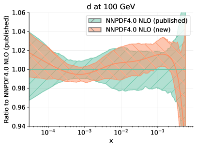
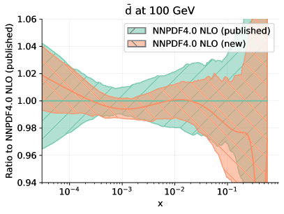
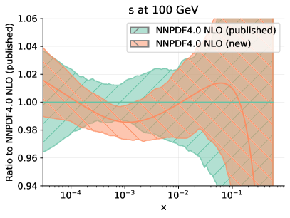
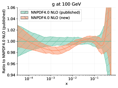
Figure A.2: The NLO PDFs at $Q=100$ GeV from the 100 replica sets compared in Table A.1 and Fig. A.1. Results are shown normalized to the central value of the published set. Bands correspond to 1$\sigma$ uncertainties. From left to right and from top to bottom, we show the up, anti-up, down, anti-down, strange and gluon PDFs.

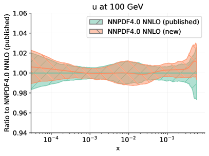
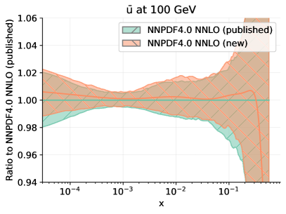
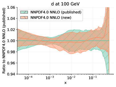
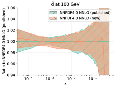
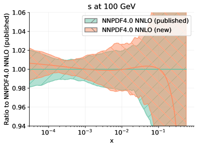
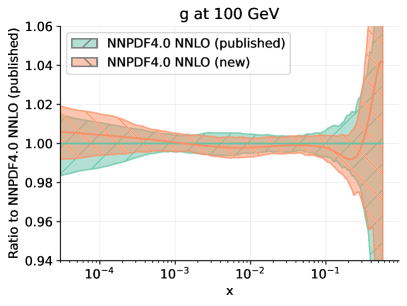
Figure A.3: Same as Fig. A.2 at NNLO.

We have generated variants of the published NNPDF4.0 NLO and NNLO fits using the new theory pipeline. In order to illustrate the equivalence between these fits and the NNPDF4.0 fits, obtained with the previous theory pipeline, we compare each pair of fits. All fits are made of 100 replicas. The corresponding statistical estimators are reported in Table A.1. In addition to the fit quality estimators, we also show the $\phi$ estimator, defined in Eq. (4.6) of Ref. [56], which measures the ratio of the average (correlated) PDF uncertainty on datapoints over the experimental uncertainty, and is thus a fairly sensitive measure of fit quality. All estimators are seen to coincide at NNLO (note that the statistical uncertainty on the $\chi^{2}$ with the given number of datapoints is 0.02), demonstrating explicitly the equivalence between the two replica sets. All estimators are also very close at NLO: differences are compatible with the statistical uncertainty on the $\chi^{2}$.

Parton distributions are compared in Fig. A.1, which displays the distances (defined in Ref. [43]) between central values and uncertainties computed using the two replica sets at $Q=100$ GeV. For a set of 100 replicas, $d\sim 1$ indicates statistical equivalence, while $d\sim 10$ indicates one-sigma differences. At NNLO, distances fluctuate about 1, indicating that the two replica sets are drawn by the same underlying distribution. At NLO, distances are somewhat larger, around the half-sigma level for most PDFs and reaching 1$\sigma$ in some cases; this is mostly due to the different FONLL implementation [54]. The PDFs themselves are shown in Figs. A.2-A.3, and the parton luminosities for the LHC at $\sqrt{s}=14$ TeV are shown in Figs. A.4-A.5, respectively at NLO and NNLO. The complete agreement between the two pairs of NNLO replica sets, and the small differences at NLO, are manifest.

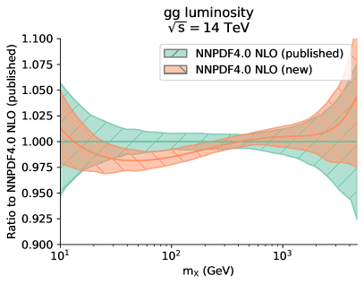
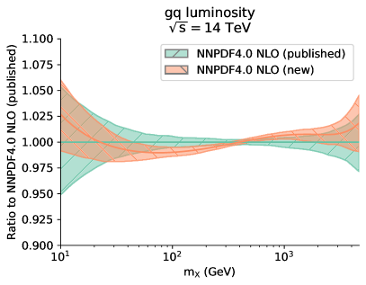
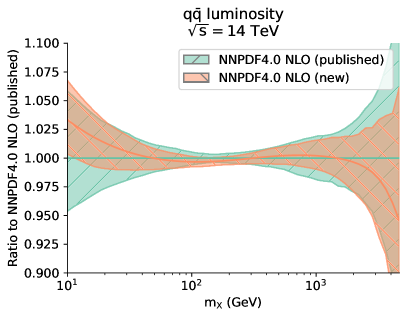
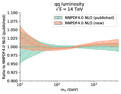
Figure A.4: Same as in Fig. A.2 for the partonic luminosities at the LHC with $\sqrt{s}=14$ TeV as a function of the invariant mass $m_{X}$. The $gg$ (left) and $qg$ (right) luminosities are shown in the top row, the $q\bar{q}$ (left), and $qq$ (right) luminosities in the bottom row.

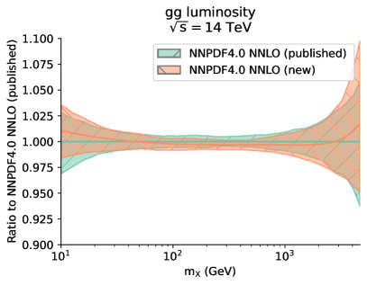
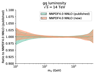
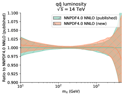
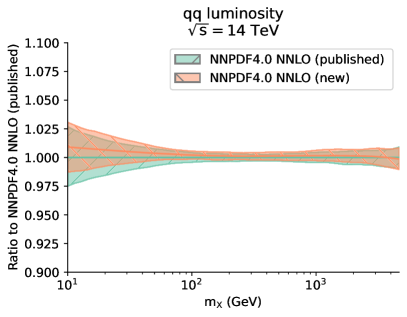
Figure A.5: Same as in Fig. A.4 at NNLO.

Appendix B Solution of evolution equations

We summarize results and benchmarks concerning the solution to evolution equations. First, we comparatively review solutions to evolution equations, for which a different choice is made in this work in comparison to the previous NNPDF3.1QED and NNPDF4.0 PDF determinations: namely the use of an exact (EXA) solution instead of the truncated (TRN) solution [28]. We then study the impact of this different choice on PDFs. Having established the equivalence of (pure QCD) PDFs obtained using either solution, we perform an inversion test of the exact QED$\times$QCD solution implemented in EKO, which we adopt, in order to verify its accuracy. We finally benchmark this EKO QED$\times$QCD solution against the implementation in the APFEL code, which was used in the previous NNPDF3.1QED PDF determination.

B.1 Exact vs. expanded solutions: formal aspects

Perturbative solutions of QCD evolution equations of the form

$$\mu^{2}\frac{df_{i}}{d\mu^{2}}=-\left(a_{s}\gamma_{ij}^{(1,0)}+a_{s}^{2}\gamma_{ij}^{(2,0)}+\dots\right)f_{j}\,,$$ (B.1)

are based on the observation that if the equation is solved exactly at leading order, with the leading-order term in the beta function Eq. (2.3), then the solution $f_{{}_{\rm LO}}(Q^{2})$ in terms of a boundary condition $f_{{}_{\rm LO}}(Q_{0}^{2})$ is a pure leading log (LL) function, i.e. it is a function of $a_{s}L$ only, where $L=\ln(Q^{2}/Q_{0}^{2})$, rather than depending on $a_{s}$ and $L$ separately. However, if the next-to leading order contributions $\gamma_{ij}^{(2,0)}$ and $\beta_{1}$ are also included, then the solution is next-to-leading log (NLL) accurate, but the exact solution Eqs. 2.16 and 2.17 includes terms to all logarithmic orders. A solution that only includes NLL terms, namely with the structure

$$f=f_{{}_{\rm LO}}+a_{s}f_{{}_{\rm NLO}},\,$$ (B.2)

where both $f_{{}_{\rm LO}}$ and $f_{{}_{\rm NLO}}$ are pure LL functions, can be constructed by linearization of the exact solution, namely by expanding the exact solution and by truncating the expansion. Various intermediate options are also possible. The argument can be repeated at any logarithmic accuracy. Of course all these solutions are equivalent up to subleading logarithmic terms.

A truncated solution to the pure QCD evolution equation of the form Eq. (B.2) can be determined in closed form to all orders in Mellin space [57], by diagonalizing order by order the anomalous dimension matrix. This corresponds to the solution referred to as truncated in Ref. [28]. However, this strategy fails for combined QED$\times$QCD evolution, because the QED and QCD anomalous dimension matrices do not commute, and thus cannot be diagonalized simultaneously. Because $a_{s}$ and $a_{em}$ depend on scale in different ways, this implies that the anomalous dimension matrices $\gamma_{ij}$ evaluated at different scales do not commute:

$$\left[\gamma\left(N,a_{s}(\mu^{2}),a_{em}(\mu^{2})\right),\gamma\left(N,a_{s}({\mu^{\prime}}^{2}),a_{em}({\mu^{\prime}}^{2})\right)\right]\not=0\quad{\rm if}\quad\mu\not=\mu^{\prime}.$$ (B.3)

This means that the LO solution, constructed only including the LO contributions to the anomalous dimensions, takes the form of a path-ordered exponential

$$f_{{}_{\rm LO}}(Q^{2})=\mathcal{P}\exp\left(-\int_{Q_{0}^{2}}^{Q^{2}}\frac{{\rm d}\mu^{2}}{\mu^{2}}\,\left(a_{s}(\mu^{2})\gamma^{(1,0)}+a_{em}(\mu^{2})\gamma^{(0,1)}\right)\right)_{{}_{\rm LO}}(Q_{0}^{2})$$ (B.4)

that cannot be written in closed form. Note that the commutator terms are not subleading: for example, the quadratic term is proportional to $a_{s}a_{em}L^{2}$, so it is a LL contribution.

The problem persists to all orders, and requires a truncated solution to be also given as a path-ordered exponential. For instance, including NLO QCD and LO QED contributions, the evolution equation is

$$\mu^{2}\frac{df_{i}}{d\mu^{2}}=-\left(a_{s}\gamma_{ij}^{(1,0)}+a_{em}\gamma_{ij}^{(0,1)}+a_{s}^{2}\gamma_{ij}^{(2,0)}\right)f_{j}\,.$$ (B.5)

The perturbative NLO QCD solution then has the form Eq. (B.2), where in the general case $f_{{}_{\rm LO}}$ and $f_{{}_{\rm NLO}}$ are LO accurate in QCD and QED, but may also include subleading contributions, i.e. $f_{{}_{\rm N^{k}LO}}=f_{{}_{\rm N^{k}LO}}(a_{s}L,a_{em}L)[1+\mathcal{O}(a_{s},a_{em})]$. Substituting the perturbative expansion Eq. (B.2) in the NLO Eq. (B.5), and using the LO solution, Eq. B.4, leads to

$$\mu^{2}\frac{df_{{}_{\rm NLO},i}}{d\mu^{2}}=-a_{s}\left(\gamma_{ij}^{(1,0)}-\beta_{{}_{\rm QCD}}^{(2,0)}\delta_{ij}\right)f_{{}_{\rm NLO},j}-a_{s}\gamma_{ij}^{(2,0)}f_{{}_{\rm LO},j}-a_{em}\gamma_{ij}^{(0,1)}f_{{}_{\rm NLO},j}\,.$$ (B.6)

Again, due to the non-commutativity of $\gamma_{ij}^{(1,0)}$ and $\gamma_{ij}^{(0,1)}$, the solution for $f_{{}_{\rm NLO}}$ is a path-ordered exponential and cannot be given in closed analytic form. This continues to be the case at higher orders.

A truncated solution can be constructed numerically, by starting with the exact path-ordered solution Eqs. (2.16-2.17), and then expanding numerically. Such an approach, however, involves approximating higher-order derivatives by finite differences [26], which may lead to numerical instabilities. This method was adopted in APFEL: APFEL is an $x$-space evolution code, so the analytic truncated solution of Ref. [57] cannot be used, and the expansion is performed numerically anyway, even in the case of pure QCD. On the other hand, in the EKO evolution code the pure QCD truncated solution is implemented through the analytic solution of Ref. [57], while the numerical path-ordered solution only needs to be used for the exact solution Eqs. 2.16 and 2.17. Therefore, in order to ensure greater accuracy, we adopt the exact solution for the QED$\times$QCD case. The impact of this choice is benchmarked in the next subsection.

B.2 Exact vs. expanded solution: impact on PDFs

We wish to quantify the impact of the choice of solution: exact, Eqs. (2.16-2.17), vs. truncated, based on an expansion of the form of Eq. (B.2). To this goal, we have determined a set of NNPDF4.0 NNLO (pure QCD) PDF replicas, but now using the exact solution, instead of the truncated solution used for the published NNPDF4.0 PDF sets. We have used the new theory pipeline.

	NNPDF4.0 NNLO QCD
	Exact Solution	Truncated Solution
$\chi^{2}$	1.17	1.17
$\left\langle E_{\rm tr}\right\rangle_{\rm rep}$	2.26 $\pm$ 0.06	2.28 $\pm$ 0.05
$\left\langle E_{\rm val}\right\rangle_{\rm rep}$	2.34 $\pm$ 0.10	2.37 $\pm$ 0.11
$\left\langle\chi^{2}\right\rangle_{\rm rep}$	1.19 $\pm$ 0.01	1.20 $\pm$ 0.02
$\left\langle{\rm TL}\right\rangle_{\rm rep}$	12100 $\pm$ 2500	12400 $\pm$ 2600
$\phi$	0.147 $\pm$ 0.005	0.153 $\pm$ 0.005

Table B.1: Same as Table A.1, now comparing a set of 100 NNPDF4.0 replicas obtained using the default truncated solution of evolution equations with a set obtained using the exact solution (pure NNLO QCD theory). Both PDF sets are produced using the new theory pipeline.

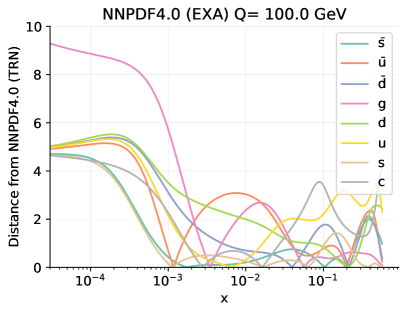
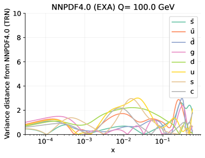
Figure B.1: Statistical distances between the central values (left) and uncertainties (right) of the 100 NNPDF4.0 PDF replicas whose statistical indicators are compared in Table B.1.

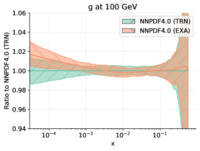
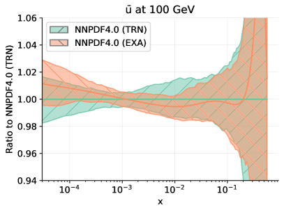
Figure B.2: The gluon (left) and anti-up quark (right) PDFs at $Q=100$ GeV from the PDF sets compared in Table B.1 and Fig. B.1. Results are shown normalized to the central value of the PDFs obtained with truncated evolution (published NNPDF4.0).

The statistical indicators for these two sets of replicas are compared in Table B.1, and are seen to be indistinguishable. The corresponding PDFs are compared in Fig. B.1, where we display the distances (defined in Ref. [43]) between the central values and uncertainties of all PDFs in either set, and in Fig. B.2, where we specifically compare the gluon and antiup PDFs at $Q=100$ GeV. It is clear that for $x\mathrel{\hbox to0.0pt{\lower 4.0pt\hbox{\hskip 1.0pt$\sim$}\hss}\raise 1.0pt\hbox{$>$}}10^{-3}$ the PDFs are statistically indistinguishable. At small $x$ they start differing at the half-$\sigma$ level, with differences at most reaching the one-$\sigma$ level for the gluon.

This is consistent with the fact that the exact and truncated solutions differ by higher-order perturbative corrections that go beyond the NNLO accuracy of the computation. Indeed, it is well known that at small $x$ the perturbative convergence starts deteriorating because of high-energy logarithms that need resummation in order for PDF determination to be accurate [58]. The qualitative behavior of the PDFs shown in Fig. B.2 agrees with this explanation: the exact solution exponentiates a set of subleading small-$x$ logarithms which are linearized in the truncated solution. It follows that in the small-$x$ region, where there is no data, these contributions lead to a stronger rise of the gluon, which then feeds back onto the quark-antiquark sea.

B.3 Exact solution: invertibility

The unexpanded EKO Eq. 2.17 manifestly satisfies the exact inversion property

$$E(Q^{2}\leftarrow Q_{0}^{2})E(Q_{0}^{2}\leftarrow Q^{2})=\mathbb{1}\,.$$ (B.7)

Hence, checking that evolving a PDF back and forth between two scales gives back the starting PDF provides a stringent test of the implementation of evolution equations and its accuracy.

We have performed this check, by starting with the NNPDF3.1QED NNLO PDFs at $Q_{a}=100$ GeV, then evolving down to $Q_{b}=1.65$ GeV and back to $Q_{a}=100$ GeV. Note that this evolution crosses back and forth the bottom quark threshold, so this also checks the accuracy of the inversion of matching conditions between the $N_{f}=4$ and $N_{f}=5$ flavor schemes. Results are displayed in Fig. B.3, where we compare the initial and final PDFs. Differences are at most at the permille level, except at very large $x$ where they can reach the percentage level, but PDFs are becoming rapidly very small. We conclude that exact evolution as implemented in the EKO code has (at least) this permille accuracy.

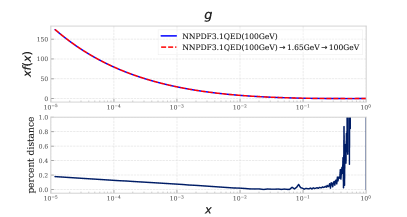
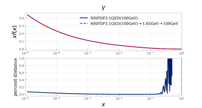
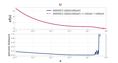
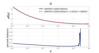
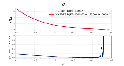
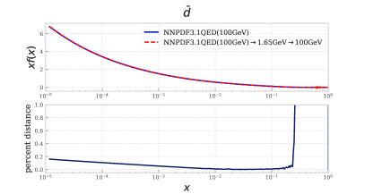
Figure B.3: Comparison between the NNPDF3.1QED PDFs at $Q_{a}=100$ GeV, with the results of evolution of the same PDFs to $Q_{b}=1.65$ GeV followed by evolution back to $Q_{a}=100$ GeV. We show, from top to bottom, the gluon, up and down (left) and the photon, anti-up and anti-down (right). In each case we show both the pair of PDFs, and their percentage relative difference.

B.4 Benchmarking of QCD$\times$QED evolution: EKO vs. APFEL

We finally compare the implementation of QCD$\times$QED evolution in the EKO code used in this paper, with the APFEL code used for the NNPDF3.1QED PDF determination. The comparison is performed by taking as input the NNPDF3.1QED NNLO PDF set at the initial parametrization scale of $Q_{0}=1.65$ GeV, evolving to $Q=100$ GeV and determining the percentage difference for all PDFs.

Results are shown in Fig. B.4 for three pairwise comparison. First, we compare APFEL exact vs. truncated evolution (green curve); the APFEL truncated result is the published NNPDF3.1 PDF set, as given by public LHAPDF grids. Then we compare EKO vs. APFEL evolution using the exact solution in both cases, and the default settings of either code as respectively used in this work and for the NNPDF3.1QED PDF set (blue curve). These settings differ in the running of the couplings: in the APFEL settings the coefficients $\beta_{{}_{\rm QCD}}^{(2,1)}$, $\beta_{{}_{\rm QED}}^{(0,3)}$ and $\beta_{{}_{\rm QED}}^{(1,2)}$ in Eqs. (2.3) and (2.4) are neglected, i.e., the two equations are decoupled and $a_{em}$ runs at leading order. Finally, we compare EKO vs. APFEL evolution using the same solution and the same settings (red curve), namely exact solution and running of the couplings as in APFEL. Note that the scale on the $y$ axis is logarithmic, and that it shows percentage difference (so $10^{-3}$ denotes a relative difference of $10^{-5}$).

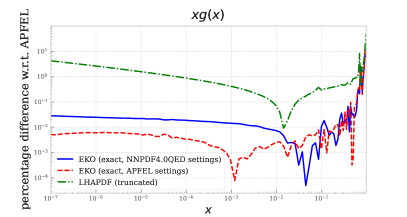
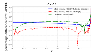
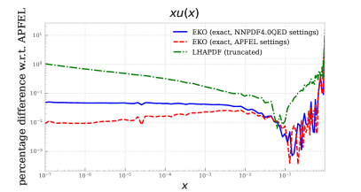
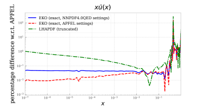
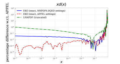
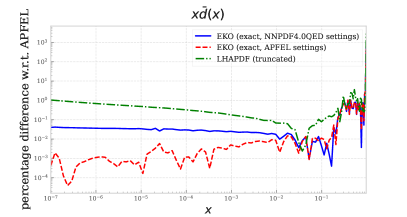
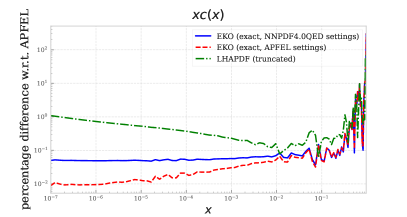
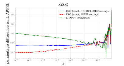
Figure B.4: Percentage difference between pairs of PDFs at $Q=100$ GeV obtained evolving NNPDF3.1QED PDFs from $Q_{0}=1.65$ GeV with different implementation of the QED$\times$QCD evolution. From top to bottom the gluon, up, down and charm (left), photon, antiup, antidown and anticharm (right) are shown. The three curves compare: APFEL exact vs. truncated evolution (green, dot-dashed); APFEL vs. EKO exact with in each case default settings for the running of the couplings (see text) (blue, solid); APFEL vs. EKO exact both with APFEL settings for the running of the coupling (red, dashed). Note the logarithmic scale on the $y$ axis; note also that the range on the $y$ axis for gluon plot differs from that of all other PDFs

The percentage differences between EKO and APFEL with common settings are always below $10^{-2}$, for all PDFs except at very large $x$ and for charm, where they are about a factor 10 larger. This sets the accuracy of the evolution codes that are being compared. The impact of the different running of the couplings is moderate: it increases the percentage difference by about a factor 3, and then only for the photon for all $x$ values, for other PDFs only at small $x\mathrel{\hbox to0.0pt{\lower 4.0pt\hbox{\hskip 1.0pt$\sim$}\hss}\raise 1.0pt\hbox{$<$}}10^{-2}$. Even so, the difference between EKO and APFEL with their respective settings is at the sub-permille level. The difference between exact and truncated evolution is at the permille level for $x\mathrel{\hbox to0.0pt{\lower 4.0pt\hbox{\hskip 1.0pt$\sim$}\hss}\raise 1.0pt\hbox{$>$}}0.003$, and it can grow up to a few percent for the gluon and a few permille for all other PDFs at very small $x\sim 10^{-6}$, in agreement with what already discussed when comparing exact and truncated evolution at the level of PDFs in Fig. B.2.

References

- [1] X. Cid Vidal et al., Report from Working Group 3: Beyond the Standard Model physics at the HL-LHC and HE-LHC, CERN Yellow Rep. Monogr. 7 (2019) 585–865, [arXiv:1812.07831].
- [2] HL-LHC, HE-LHC Working Group Collaboration, P. Azzi et al., Standard Model Physics at the HL-LHC and HE-LHC, arXiv:1902.04070.
- [3] Physics of the HL-LHC Working Group Collaboration, M. Cepeda et al., Higgs Physics at the HL-LHC and HE-LHC, arXiv:1902.00134.
- [4] G. Heinrich, Collider Physics at the Precision Frontier, Phys. Rept. 922 (2021) 1–69, [arXiv:2009.00516].
- [5] V. Bertone, S. Carrazza, D. Pagani, and M. Zaro, On the Impact of Lepton PDFs, JHEP 11 (2015) 194, [arXiv:1508.07002].
- [6] B. Fornal, A. V. Manohar, and W. J. Waalewijn, Electroweak Gauge Boson Parton Distribution Functions, JHEP 05 (2018) 106, [arXiv:1803.06347].
- [7] C. W. Bauer, N. Ferland, and B. R. Webber, Standard Model Parton Distributions at Very High Energies, JHEP 08 (2017) 036, [arXiv:1703.08562].
- [8] M. McCullough, J. Moore, and M. Ubiali, The dark side of the proton, JHEP 08 (2022) 019, [arXiv:2203.12628].
- [9] A. D. Martin, R. G. Roberts, W. J. Stirling, and R. S. Thorne, Parton distributions incorporating QED contributions, Eur. Phys. J. C39 (2005) 155, [hep-ph/0411040].
- [10] C. Schmidt, J. Pumplin, D. Stump, and C. P. Yuan, CT14QED parton distribution functions from isolated photon production in deep inelastic scattering, Phys. Rev. D93 (2016), no. 11 114015, [arXiv:1509.02905].
- [11] R. D. Ball et al., Parton distributions with LHC data, Nucl.Phys. B867 (2013) 244, [arXiv:1207.1303].
- [12] NNPDF Collaboration, R. D. Ball et al., Parton distributions with QED corrections, Nucl.Phys. B877 (2013) 290–320, [arXiv:1308.0598].
- [13] xFitter Developers’ Team Collaboration, F. Giuli et al., The photon PDF from high-mass Drell–Yan data at the LHC, Eur. Phys. J. C77 (2017), no. 6 400, [arXiv:1701.08553].
- [14] ATLAS Collaboration, G. Aad et al., Measurement of the double-differential high-mass Drell-Yan cross section in pp collisions at TeV with the ATLAS detector, JHEP 08 (2016) 009, [arXiv:1606.01736].
- [15] A. Manohar, P. Nason, G. P. Salam, and G. Zanderighi, How bright is the proton? A precise determination of the photon parton distribution function, Phys. Rev. Lett. 117 (2016), no. 24 242002, [arXiv:1607.04266].
- [16] A. V. Manohar, P. Nason, G. P. Salam, and G. Zanderighi, The Photon Content of the Proton, JHEP 12 (2017) 046, [arXiv:1708.01256].
- [17] L. A. Harland-Lang, V. A. Khoze, and M. G. Ryskin, Photon-initiated processes at high mass, Phys. Rev. D 94 (2016), no. 7 074008, [arXiv:1607.04635].
- [18] L. A. Harland-Lang, V. A. Khoze, and M. G. Ryskin, Sudakov effects in photon-initiated processes, Phys. Lett. B761 (2016) 20–24, [arXiv:1605.04935].
- [19] NNPDF Collaboration, V. Bertone, S. Carrazza, N. P. Hartland, and J. Rojo, Illuminating the photon content of the proton within a global PDF analysis, SciPost Phys. 5 (2018), no. 1 008, [arXiv:1712.07053].
- [20] L. A. Harland-Lang, A. D. Martin, R. Nathvani, and R. S. Thorne, Ad Lucem: QED Parton Distribution Functions in the MMHT Framework, Eur. Phys. J. C 79 (2019), no. 10 811, [arXiv:1907.02750].
- [21] T. Cridge, L. A. Harland-Lang, A. D. Martin, and R. S. Thorne, QED parton distribution functions in the MSHT20 fit, Eur. Phys. J. C 82 (2022), no. 1 90, [arXiv:2111.05357].
- [22] K. Xie, T. Hobbs, T.-J. Hou, C. Schmidt, M. Yan, and C.-P. Yuan, The photon content of the proton in the CT18 global analysis, SciPost Phys. Proc. 8 (2022) 074, [arXiv:2107.13580].
- [23] K. Xie, B. Zhou, and T. J. Hobbs, The Photon Content of the Neutron, arXiv:2305.10497.
- [24] NNPDF Collaboration, R. D. Ball et al., The path to proton structure at 1% accuracy, Eur. Phys. J. C 82 (2022), no. 5 428, [arXiv:2109.02653].
- [25] NNPDF Collaboration, R. D. Ball et al., An open-source machine learning framework for global analyses of parton distributions, Eur. Phys. J. C 81 (2021), no. 10 958, [arXiv:2109.02671].
- [26] V. Bertone, S. Carrazza, and J. Rojo, APFEL: A PDF Evolution Library with QED corrections, Comput.Phys.Commun. 185 (2014) 1647, [arXiv:1310.1394].
- [27] V. Bertone, S. Carrazza, and N. P. Hartland, APFELgrid: a high performance tool for parton density determinations, Comput. Phys. Commun. 212 (2017) 205–209, [arXiv:1605.02070].
- [28] A. Candido, F. Hekhorn, and G. Magni, EKO: evolution kernel operators, Eur. Phys. J. C 82 (2022), no. 10 976, [arXiv:2202.02338].
- [29] A. Candido, F. Hekhorn, G. Magni, T. Rabemananjara, and R. Stegeman, YADISM: Yet Another DIS Module, . In preparation.
- [30] C. Schwan, A. Candido, F. Hekhorn, S. Carrazza, and A. Barontini, Nnpdf/pineappl: v0.6.0, June, 2023.
- [31] S. Carrazza, E. R. Nocera, C. Schwan, and M. Zaro, PineAPPL: combining EW and QCD corrections for fast evaluation of LHC processes, JHEP 12 (2020) 108, [arXiv:2008.12789].
- [32] A. Barontini, A. Candido, J. M. Cruz-Martinez, F. Hekhorn, and C. Schwan, Pineline: Industrialization of high-energy theory predictions, Comput. Phys. Commun. 297 (2024) 109061, [arXiv:2302.12124].
- [33] R. Frederix, S. Frixione, V. Hirschi, D. Pagani, H. S. Shao, and M. Zaro, The automation of next-to-leading order electroweak calculations, JHEP 07 (2018) 185, [arXiv:1804.10017]. [Erratum: JHEP 11, 085 (2021)].
- [34] A. Vogt, S. Moch, and J. A. M. Vermaseren, The Three-loop splitting functions in QCD: The Singlet case, Nucl. Phys. B 691 (2004) 129–181, [hep-ph/0404111].
- [35] S. Moch, J. A. M. Vermaseren, and A. Vogt, The Three loop splitting functions in QCD: The Nonsinglet case, Nucl. Phys. B 688 (2004) 101–134, [hep-ph/0403192].
- [36] D. de Florian, G. F. R. Sborlini, and G. Rodrigo, Two-loop QED corrections to the Altarelli-Parisi splitting functions, JHEP 10 (2016) 056, [arXiv:1606.02887].
- [37] D. de Florian, G. F. R. Sborlini, and G. Rodrigo, QED corrections to the Altarelli–Parisi splitting functions, Eur. Phys. J. C76 (2016), no. 5 282, [arXiv:1512.00612].
- [38] L. R. Surguladze, O(alpha**n alpha-s**m) corrections in e+ e- annihilation and tau decay, hep-ph/9803211.
- [39] S. Fanchiotti, B. A. Kniehl, and A. Sirlin, Incorporation of QCD effects in basic corrections of the electroweak theory, Phys. Rev. D 48 (1993) 307–331, [hep-ph/9212285].
- [40] A. Denner and S. Dittmaier, Electroweak Radiative Corrections for Collider Physics, Phys. Rept. 864 (2020) 1–163, [arXiv:1912.06823].
- [41] R. D. Ball, M. Bonvini, and L. Rottoli, Charm in Deep-Inelastic Scattering, JHEP 11 (2015) 122, [arXiv:1510.02491].
- [42] CTEQ-TEA Collaboration, K. Xie, T. J. Hobbs, T.-J. Hou, C. Schmidt, M. Yan, and C. P. Yuan, Photon PDF within the CT18 global analysis, Phys. Rev. D 105 (2022), no. 5 054006, [arXiv:2106.10299].
- [43] The NNPDF Collaboration, R. D. Ball et al., A first unbiased global NLO determination of parton distributions and their uncertainties, Nucl. Phys. B838 (2010) 136, [arXiv:1002.4407].
- [44] The NNPDF Collaboration, R. D. Ball et al., Fitting Parton Distribution Data with Multiplicative Normalization Uncertainties, JHEP 05 (2010) 075, [arXiv:0912.2276].
- [45] T. Cridge, L. A. Harland-Lang, and R. S. Thorne, Combining QED and Approximate N3LO QCD Corrections in a Global PDF Fit: MSHT20qed_an3lo PDFs, arXiv:2312.07665.
- [46] NNPDF Collaboration, R. Abdul Khalek et al., A first determination of parton distributions with theoretical uncertainties, Eur. Phys. J. C (2019) 79:838, [arXiv:1905.04311].
- [47] NNPDF Collaboration, R. Abdul Khalek et al., Parton Distributions with Theory Uncertainties: General Formalism and First Phenomenological Studies, Eur. Phys. J. C 79 (2019), no. 11 931, [arXiv:1906.10698].
- [48] F. Hekhorn and G. Magni, DGLAP evolution of parton distributions at approximate N3LO, arXiv:2306.15294.
- [49] R. D. Ball, A. Candido, S. Forte, F. Hekhorn, E. R. Nocera, J. Rojo, and C. Schwan, Parton distributions and new physics searches: the Drell–Yan forward–backward asymmetry as a case study, Eur. Phys. J. C 82 (2022), no. 12 1160, [arXiv:2209.08115].
- [50] E. Hammou, Z. Kassabov, M. Madigan, M. L. Mangano, L. Mantani, J. Moore, M. M. Alvarado, and M. Ubiali, Hide and seek: how PDFs can conceal new physics, JHEP 11 (2023) 090, [arXiv:2307.10370].
- [51] T. Carli et al., A posteriori inclusion of parton density functions in NLO QCD final-state calculations at hadron colliders: The APPLGRID Project, Eur.Phys.J. C66 (2010) 503, [arXiv:0911.2985].
- [52] fastNLO Collaboration, M. Wobisch, D. Britzger, T. Kluge, K. Rabbertz, and F. Stober, Theory-Data Comparisons for Jet Measurements in Hadron-Induced Processes, arXiv:1109.1310.
- [53] A. Candido, A. Garcia, G. Magni, T. Rabemananjara, J. Rojo, and R. Stegeman, Neutrino Structure Functions from GeV to EeV Energies, JHEP 05 (2023) 149, [arXiv:2302.08527].
- [54] A. Barontini, A. Candido, F. Hekhorn, G. Magni, and R. Stegeman, An FONLL prescription with coexisting flavor number PDFs, . in preparation.
- [55] C. Anastasiou, L. J. Dixon, K. Melnikov, and F. Petriello, High precision QCD at hadron colliders: Electroweak gauge boson rapidity distributions at NNLO, Phys. Rev. D69 (2004) 094008, [hep-ph/0312266].
- [56] NNPDF Collaboration, R. D. Ball et al., Parton distributions for the LHC Run II, JHEP 04 (2015) 040, [arXiv:1410.8849].
- [57] A. Vogt, Efficient evolution of unpolarized and polarized parton distributions with qcd-pegasus, Comput. Phys. Commun. 170 (2005) 65–92, [hep-ph/0408244].
- [58] R. D. Ball, V. Bertone, M. Bonvini, S. Marzani, J. Rojo, and L. Rottoli, Parton distributions with small-x resummation: evidence for BFKL dynamics in HERA data, Eur. Phys. J. C78 (2018), no. 4 321, [arXiv:1710.05935].