Infinitesimal and infinite numbers in applied mathematics

Abstract.

The need to describe abrupt changes or response of nonlinear systems to impulsive stimuli is ubiquitous in applications. Also the informal use of infinitesimal and infinite quantities is still a method used to construct idealized but tractable models within the famous J. von Neumann reasonably wide area of applicability. We review the theory of generalized smooth functions as a candidate to address both these needs: a rigorous but simple language of infinitesimal and infinite quantities, and the possibility to deal with continuous and generalized function as if they were smooth maps: with pointwise values, free composition and hence nonlinear operations, all the classical theorems of calculus, a good integration theory, and new existence results for differential equations. We exemplify the applications of this theory through several models of singular dynamical systems: deduction of the heat and wave equations extended to generalized functions, a singular variable length pendulum wrapping on a parallelepiped, the oscillation of a pendulum damped by different media, a nonlinear stress-strain model of steel, singular Lagrangians as used in optics, and some examples from quantum mechanics.

1. Introduction: informal uses of infinitesimals and infinities in applied mathematics

Even if infinitesimal numbers have been banished by modern mathematics, several physicists, engineers and mathematicians still profitably continue to use them. Usually, this is in order to simplify calculations, to construct idealized but notwithstanding interesting models of physical systems, or to relate different parts of physics, such as in passing from quantum to classical mechanics if $\hbar$ is infinitesimal. An authoritative example in this direction is given by A. Einstein when he writes

$$\frac{1}{\sqrt{1-{\displaystyle\frac{v^{2}}{c^{2}}}}}=1+\frac{v^{2}}{2c^{2}}\qquad\qquad\sqrt{1-h_{44}(x)}=1-\frac{1}{2}h_{44}(x)$$ (1.1)

with explicit use of infinitesimals $v/c\ll 1$ or $h_{44}(x)\ll 1$ such that e.g. $h_{44}(x)^{2}=0$. More generally, in [21] Einstein writes the formula (using the equality sign and not the approximate equality sign $\simeq$)

$$f(x,t+\tau)=f(x,t)+\tau\cdot\frac{\partial f}{\partial t}(x,t)$$ (1.2)

justifying it with the words “since $\tau$ is very small”; note that (1.1) are a particular case of the general (1.2). Also P.A.M. Dirac in [18] writes an analogous equality studying the Newtonian approximation in general relativity.

A certain degree of inconsistency appears also at the level of elementary topics, e.g. in the deduction of the wave and heat equations, see e.g. [75]. For example, if $u(x,t)$ is the string displacement, then formula (1.2) is once again used e.g. “to ignore magnitudes of order greater than $\frac{\partial u}{\partial x}$”. This means that we need to have $\left(\frac{\partial u}{\partial x}\right)^{2}=0$ to arrive at the final equation with an equality sign and not with some kind of approximation $\simeq$. But then the length of the string becomes

$$L=\int_{a}^{b}\sqrt{1+\left[\frac{\partial u}{\partial x}(x,t)\right]^{2}}\,\mathchoice{\hbox{\rm d}x}{\hbox{\rm d}x}{\scalebox{0.75}{$\hbox{\rm d}x$}}{\scalebox{0.35}{$\hbox{\rm d}x$}}=b-a,$$

and its clear that this necessarily yields that the function $u$ is constant. It clearly does not really help to use $\simeq$ when we have a contradiction, but then to change it into $=$ when we need the final equation. It is for this type of motivations that V.I. Arnol’d in [2] wrote: Nowadays, when teaching analysis, it is not very popular to talk about infinitesimal quantities. Consequently present-day students are not fully in command of this language. Nevertheless, it is still necessary to have command of it.

A similar, but sometimes more troublesome, practice concerns the use of infinite numbers. A typical example is given by Heisenberg’s uncertainty principle

$$\Delta p_{x}\Delta x\geq\frac{\hbar}{2}.$$ (1.3)

It is frequently informally argued that if the position $x$ is measured by a Dirac delta, then $\Delta x\approx 0$ is infinitesimal; thereby, (1.3) necessarily implies that $\Delta p_{x}$ must be an infinite number.

Another classical example of informal use of infinite numbers concerns Schwartz distributions and their point values. Many relevant physical systems are in fact described by singular Hamiltonians. Among them, we can e.g. list:

1. Non smooth classical mechanics. For example, a classical particle (or a high-frequency wave) moving through discontinuous media containing barriers or interfaces where the Hamiltonian is discontinuous: see e.g. [7, 8, 16, 73, 39, 68, 70] and references therein.

2. Discontinuous Lagrangian in geometrical optics: see e.g. [46].

3. Nonlinear deformation in continuum mechanics, which includes non differentiable stress-strain relations: see e.g. [74, 10].

4. The use of infinite quantities in quantum mechanics. An elementary example is given by the solution of the stationary Schrödinger equation for an infinite rectangular potential well (a case that cannot be formalized using Schwartz distributions, see e.g. [24]).

This type of problems is hence widely studied from the mathematical point of view (see e.g. [15, 52, 50, 71, 44, 43, 51]), even if the presented solutions are not general and hold only in special conditions. In this sense, the fact that J.D. Marsden’s works [54, 55] did not start a consolidated research thread to study singular Hamiltonian mechanics using Schwartz distributions, can be considered as a clue that the classical distributional framework is not well suited to face this problem in general terms.

A related problem concerns nonlinear operations on Schwartz distributions, which can be simply presented as follows. Let $A$ be an associative and commutative algebra endowed with a derivation (satisfying the Leibniz rule). Then any element $H$ of $A$ such that $H\cdot H=H$ is necessarily a constant, that is, $H^{\prime}=0$. Indeed, $(H^{2})^{\prime}=2HH^{\prime}$ and $(H^{3})^{\prime}=3H^{2}H^{\prime}$ . Now $H=H^{2}=H^{3}$ , so this implies $2HH^{\prime}=H^{\prime}=3HH^{\prime}$ . Therefore, $HH^{\prime}=0$ and hence also $H^{\prime}=2HH^{\prime}=0$. Even worse, we also recall that Dirac in [19] uses terms of the form $\sqrt{\delta}$ in his proposal for the foundation of quantum mechanics.

There are obviously many possibilities to formalize this kind of intuitive reasonings, obtaining a more or less good dialectic between informal and formal thinking, and nowadays there are indeed several rigorous theories of infinitesimals, infinities and generalized functions. Concerning the notion of infinitesimal, we can distinguish two definitions: in the first one we have at least a ring $R$ containing the real field $\mathbb{R}$ and infinitesimals are elements $h\in R$ such that $-r<h<r$ for every positive standard real $r\in\mathbb{R}_{>0}$. The second type of infinitesimal is defined using some algebraic property of nilpotency, i.e. $h^{n}=0$ for some natural number $n\in\mathbb{N}$ (therefore, in this case $h$ cannot be trivially invertible and we cannot form infinities as reciprocal of infinitesimals). For some ring $R$ these definitions can coincide, but anyway they lead, of course, only to the trivial infinitesimal $h=0$ if $R=\mathbb{R}$ is the real field.

Mathematical theories of infinitesimals can also be classified as belonging to two different classes. In the first one, we have theories needing a certain amount of non trivial results of mathematical logic, whereas in the second one we have attempts to define sufficiently strong theories of infinitesimals without the use of non trivial results of mathematical logic. In the first class, we can list nonstandard analysis and synthetic differential geometry (also called smooth infinitesimal analysis, see e.g. [3, 42, 48, 57]), in the second one we have, e.g., Weil functors (see [45]), Levi-Civita field (see [69]), surreal numbers (see [14]), Fermat reals (see [26]), Colombeau’s generalized numbers (see [13] and [20, 40] for a general survey). More precisely, we can say that to work both in nonstandard analysis and in synthetic differential geometry, one needs a formal control stronger than the one used in “standard mathematics”. Indeed, to use nonstandard analysis one has to be able to formally write sentences in order to apply the transfer theorem. Whereas synthetic differential geometry does not admit models in classical logic, but in intuitionistic logic only, and hence we have to be sure that in our proofs there is no use of the law of the excluded middle, or e.g. of the classical part of De Morgan’s law or of some form of the axiom of choice or of the implication of double negation toward affirmation and any other logical principle which do not hold in intuitionistic logic. Physicists, engineers, but also the greatest part of mathematicians are not used to have this strong formal control in their work, and it is for this reason that there are attempts to present both nonstandard analysis and synthetic differential geometry reducing as much as possible the necessary formal control, even if at some level this is technically impossible (see e.g. [41, 35], and [4, 5] for nonstandard analysis; [3] and [48] for synthetic differential geometry).

On the other hand, nonstandard analysis is surely the best known theory of invertible infinitesimals with results in several areas of mathematics and its applications, see e.g. [1]. Synthetic differential geometry is a theory of nilpotent infinitesimals with non trivial results of differential geometry in infinite dimensional spaces.

Concerning mathematical theories of generalized functions, the difficulties stemmed from dealing with the lacking of well-posedness in PDE initial value problems led to a zoo of spaces of generalized functions. In an incomplete list we can mention: Schwartz distributions, Colombeau generalized functions, ultradistributions, hyperfunctions, nonstandard theory of Colombeau generalized functions, ultrafunctions, etc. See e.g. [38] for a survey, and the International Conference on Generalized Functions series, e.g. https://ps-mathematik.univie.ac.at/e/index.php?event=GF2022.

Unfortunately, there is a certain lacking of dialog between the most used theory of generalized functions, i.e. Schwartz distributions, and the actual use of generalized functions in physics and engineering, where e.g. point values and nonlinear operations are frequently needed, see e.g. [13].

In the present paper, we describe the main results of generalized smooth functions (GSF) theory and some of its applications in applied mathematics. GSF are an extension of classical distribution theory and of Colombeau theory, which makes it possible to model nonlinear singular problems, while at the same time sharing a number of fundamental properties with ordinary smooth functions, such as the closure with respect to composition and several non trivial classical theorems of the calculus, see [30, 31, 28, 27, 53, 32]. One could describe GSF as a methodological restoration of Cauchy-Dirac’s original conception of generalized function (GF), see [47]. In essence, the idea of Cauchy and Dirac (but also of Poisson, Kirchhoff, Helmholtz, Kelvin and Heaviside) was to view generalized functions as suitable types of smooth set-theoretical maps obtained from ordinary smooth maps depending on suitable infinitesimal or infinite parameters.

The calculus of GSF is closely related to classical analysis, in fact:

1. GSF are set-theoretical maps defined on, and attaining values in the non-Archimedean ring $\mathchoice{{\vphantom{\mathbb{R}}}^{\scalebox{0.6}{$\rho$}}}{{\vphantom{\mathbb{R}}}^{\scalebox{0.56}{$\rho$}}}{{\vphantom{\mathbb{R}}}^{\scalebox{0.47}{$\rho$}}}{{\vphantom{\mathbb{R}}}^{\scalebox{0.35}{$\rho$}}}\widetilde{\mathbb{R}}$ of Robinson-Colombeau. Therefore, in $\mathchoice{{\vphantom{\mathbb{R}}}^{\scalebox{0.6}{$\rho$}}}{{\vphantom{\mathbb{R}}}^{\scalebox{0.56}{$\rho$}}}{{\vphantom{\mathbb{R}}}^{\scalebox{0.47}{$\rho$}}}{{\vphantom{\mathbb{R}}}^{\scalebox{0.35}{$\rho$}}}\widetilde{\mathbb{R}}$ we have infinitesimals, infinities and also a suitable language of nilpotent infinitesimals, see Sec. 2, Sec. 3.

2. GSF include all Colombeau generalized functions and hence also all Schwartz distributions, see Sec. 3.

3. They allow nonlinear operations on GF and to compose them unrestrictedly, so that terms such as $\delta^{2}(x)$ or even $\delta(\delta(x))$ are possible, see Sec. 3.

4. GSF allow us to prove a number of analogues of theorems of classical analysis: e.g., mean value theorem, intermediate value theorem, extreme value theorem, Taylor’s theorem, local and global inverse function theorem, integrals via primitives, multidimensional integrals, theory of compactly supported GF. Therefore, this approach to GF results in a flexible and rich framework which allows both the formalization of calculations appearing in physics and engineering and the development of new applications in mathematics and mathematical physics. Some of these results are presented in Sec. 3.

5. Several results of the classical theory of calculus of variations and optimal control can be developed for GSF: the fundamental lemma, second variation and minimizers, necessary Legendre condition, Jacobi fields, conjugate points and Jacobi’s theorem, Noether’s theorem, see [49, 23].

6. The closure with respect to composition leads to a solution concept of differential equations close to the classical one. In GSF theory, we have a non-Archimedean version of the Banach fixed point theorem, a Picard-Lindelöf theorem for both ODE and PDE, results about the maximal set of existence, Gronwall theorem, flux properties, continuous dependence on initial conditions, full compatibility with classical smooth solutions, etc., see Sec. 4.

As we will see in Sec. 5 and Sec. 6, using GSF theory, we have a rigorous theory of infinitesimal and infinite numbers that can be used to develop mathematical models of physical problems. On the other hand, it is also a flexible theory of GF that can be used to model situations with singular (non smooth) physical quantities. One of the main aim of this paper is to show that within GSF theory several informal calculations of physics or engineering now become perfectly rigorous without detaching too much from the original deduction.

The structure of the paper is as follows: in Sec. 2, we introduce our new ring of scalars $\mathchoice{{\vphantom{\mathbb{R}}}^{\scalebox{0.6}{$\rho$}}}{{\vphantom{\mathbb{R}}}^{\scalebox{0.56}{$\rho$}}}{{\vphantom{\mathbb{R}}}^{\scalebox{0.47}{$\rho$}}}{{\vphantom{\mathbb{R}}}^{\scalebox{0.35}{$\rho$}}}\widetilde{\mathbb{R}}$, the ring of Robinson-Colombeau. In Sec. 3, we define GSF as suitable set-theoretical functions defined and valued in the new ring of scalars; we will also see the relationships with Colombeau GF and hence with Schwartz distributions. In Sec. 4, we see the Picard-Lindelöf theorem for singular nonlinear ODE involving GSF. In Sec. 5, we see how to transform the classical deductions of the wave and heat equations into formal mathematical theorems whose scope includes GSF. Finally, in Sec. 6 we see applications to non-smooth mechanics, an empirical non-linear stress-strain model for steel, some applications in optics with discontinuous Lagrangians, how to see the classical finite and infinite potential wells of QM within GSF theory.

The paper is a review of GSF theory, so it is self-contained in the sense that it contains all the statements required for the proofs of Sec. 5 and Sec. 6. We also introduce clear intuitions about the new mathematical objects of this theory and references for the complete proofs. Therefore, to understand this paper, only a basic knowledge of distribution theory is needed.

2. Numbers: The ring of Robinson-Colombeau

In this first section, we introduce our non-Archimedean ring of scalars. More in depth details about the basic notions and the omitted proofs as well can be found in [31, 30].

Definition 1.

Let $I:=(0,1]$ and $\rho=(\rho_{\varepsilon})\in(0,1]^{I}$ be a net such that $(\rho_{\varepsilon})\to 0$ as $\varepsilon\to 0^{+}$ (in the following, such a net will be called a gauge), then

1. $\mathcal{I}(\rho):=\left\{(\rho_{\varepsilon}^{-a})\mid a\in\mathbb{R}_{>0}\right\}$ is called the asymptotic gauge generated by $\rho$.

2. If $\mathcal{P}(\varepsilon)$ is a property of $\varepsilon\in I$, we use the notation $\forall^{0}\varepsilon:\,\mathcal{P}(\varepsilon)$ to denote $\exists\varepsilon_{0}\in I\,\forall\varepsilon\in(0,\varepsilon_{0}]:\,\mathcal{P}(\varepsilon)$. We can read $\forall^{0}\varepsilon$ as: “for $\varepsilon$ small”.

3. We say that a net $(x_{\varepsilon})\in\mathbb{R}^{I}$ is $\rho$-moderate, and we write $(x_{\varepsilon})\in\mathbb{R}_{\rho}$, if

   $$\exists(J_{\varepsilon})\in\mathcal{I}(\rho):\ x_{\varepsilon}=O(J_{\varepsilon})\text{ as }\varepsilon\to 0^{+},$$ (2.1)

   i.e., if

   $$\exists N\in\mathbb{N}\,\forall^{0}\varepsilon:\ |x_{\varepsilon}|\leq\rho_{\varepsilon}^{-N}.$$

4. Let $(x_{\varepsilon})$, $(y_{\varepsilon})\in\mathbb{R}^{I}$, then we say that $(x_{\varepsilon})\sim_{\rho}(y_{\varepsilon})$ if

   $$\forall(J_{\varepsilon})\in\mathcal{I}(\rho):\ x_{\varepsilon}=y_{\varepsilon}+O(J_{\varepsilon}^{-1})\text{ as }\varepsilon\to 0^{+},$$

   that is if

   $$\forall n\in\mathbb{N}\,\forall^{0}\varepsilon:\ |x_{\varepsilon}-y_{\varepsilon}|\leq\rho_{\varepsilon}^{n}.$$ (2.2)

   This is a congruence relation on the ring $\mathbb{R}_{\rho}$ of moderate nets with respect to pointwise operations, and we can hence define

   $$\mathchoice{{\vphantom{\mathbb{R}}}^{\scalebox{0.6}{$\rho$}}}{{\vphantom{\mathbb{R}}}^{\scalebox{0.56}{$\rho$}}}{{\vphantom{\mathbb{R}}}^{\scalebox{0.47}{$\rho$}}}{{\vphantom{\mathbb{R}}}^{\scalebox{0.35}{$\rho$}}}\widetilde{\mathbb{R}}:=\mathbb{R}_{\rho}/\sim_{\rho},$$ (2.3)

   which we call Robinson-Colombeau ring of generalized numbers.

This name is justified by [66, 13]: Indeed, in [66] A. Robinson introduced the notion of moderate and negligible nets depending on an arbitrary fixed infinitesimal $\rho$ (in the framework of nonstandard analysis); independently, J.F. Colombeau, cf. e.g. [13] and references therein, studied the same concepts without using nonstandard analysis, but considering only the particular infinitesimal $\rho_{\varepsilon}=\varepsilon$. Equivalence classes of the quotient ring (2.3) are simply denoted with $[x_{\varepsilon}]:=[(x_{\varepsilon})_{\varepsilon}]_{\sim_{\rho}}\in\mathchoice{{\vphantom{\mathbb{R}}}^{\scalebox{0.6}{$\rho$}}}{{\vphantom{\mathbb{R}}}^{\scalebox{0.56}{$\rho$}}}{{\vphantom{\mathbb{R}}}^{\scalebox{0.47}{$\rho$}}}{{\vphantom{\mathbb{R}}}^{\scalebox{0.35}{$\rho$}}}\widetilde{\mathbb{R}}$.

Considering constant net $x_{\varepsilon}=r\in\mathbb{R}$ we have the embedding $\mathbb{R}\subset\mathchoice{{\vphantom{\mathbb{R}}}^{\scalebox{0.6}{$\rho$}}}{{\vphantom{\mathbb{R}}}^{\scalebox{0.56}{$\rho$}}}{{\vphantom{\mathbb{R}}}^{\scalebox{0.47}{$\rho$}}}{{\vphantom{\mathbb{R}}}^{\scalebox{0.35}{$\rho$}}}\widetilde{\mathbb{R}}$. We define $[x_{\varepsilon}]\leq[y_{\varepsilon}]$ if there exists $(z_{\varepsilon})\in\mathbb{R}^{I}$ such that $(z_{\varepsilon})\sim_{\rho}0$ (we then say that $(z_{\varepsilon})$ is $\rho$-negligible) and $x_{\varepsilon}\leq y_{\varepsilon}+z_{\varepsilon}$ for $\varepsilon$ small. Equivalently, we have that $x\leq y$ if and only if there exist representatives $[x_{\varepsilon}]=x$ and $[y_{\varepsilon}]=y$ such that $x_{\varepsilon}\leq y_{\varepsilon}$ for all $\varepsilon$. A proficient intuitive point of view on these generalized numbers is to think at $[x_{\varepsilon}]\in\mathchoice{{\vphantom{\mathbb{R}}}^{\scalebox{0.6}{$\rho$}}}{{\vphantom{\mathbb{R}}}^{\scalebox{0.56}{$\rho$}}}{{\vphantom{\mathbb{R}}}^{\scalebox{0.47}{$\rho$}}}{{\vphantom{\mathbb{R}}}^{\scalebox{0.35}{$\rho$}}}\widetilde{\mathbb{R}}$ as a dynamic point in the time $\varepsilon\to 0^{+}$; classical real numbers are hence static points. We say that $x=[x_{\varepsilon}]\in\mathchoice{{\vphantom{\mathbb{R}}}^{\scalebox{0.6}{$\rho$}}}{{\vphantom{\mathbb{R}}}^{\scalebox{0.56}{$\rho$}}}{{\vphantom{\mathbb{R}}}^{\scalebox{0.47}{$\rho$}}}{{\vphantom{\mathbb{R}}}^{\scalebox{0.35}{$\rho$}}}\widetilde{\mathbb{R}}$ is near-standard if $\exists\lim_{\varepsilon\to 0^{+}}x_{\varepsilon}=:{x^{\circ}}\in\mathbb{R}$.

Even though the order $\leq$ is not total, we still have the possibility to define the infimum $[x_{\varepsilon}]\wedge[y_{\varepsilon}]:=[\min(x_{\varepsilon},y_{\varepsilon})]$, the supremum $[x_{\varepsilon}]\vee[y_{\varepsilon}]:=\left[\max(x_{\varepsilon},y_{\varepsilon})\right]$ of a finite amount of generalized numbers. Henceforth, we will also use the customary notation $\mathchoice{{\vphantom{\mathbb{R}}}^{\scalebox{0.6}{$\rho$}}}{{\vphantom{\mathbb{R}}}^{\scalebox{0.56}{$\rho$}}}{{\vphantom{\mathbb{R}}}^{\scalebox{0.47}{$\rho$}}}{{\vphantom{\mathbb{R}}}^{\scalebox{0.35}{$\rho$}}}\widetilde{\mathbb{R}}^{*}$ for the set of invertible generalized numbers, and we write $x<y$ to say that $x\leq y$ and $x-y\in\mathchoice{{\vphantom{\mathbb{R}}}^{\scalebox{0.6}{$\rho$}}}{{\vphantom{\mathbb{R}}}^{\scalebox{0.56}{$\rho$}}}{{\vphantom{\mathbb{R}}}^{\scalebox{0.47}{$\rho$}}}{{\vphantom{\mathbb{R}}}^{\scalebox{0.35}{$\rho$}}}\widetilde{\mathbb{R}}^{*}$, i.e. if $x$ is less of equal to $y$ and $x-y$ is invertible. The intervals are denoted by: $[a,b]:=\{x\in\mathchoice{{\vphantom{\mathbb{R}}}^{\scalebox{0.6}{$\rho$}}}{{\vphantom{\mathbb{R}}}^{\scalebox{0.56}{$\rho$}}}{{\vphantom{\mathbb{R}}}^{\scalebox{0.47}{$\rho$}}}{{\vphantom{\mathbb{R}}}^{\scalebox{0.35}{$\rho$}}}\widetilde{\mathbb{R}}\mid a\leq x\leq b\}$, $[a,b]_{\mathbb{R}}:=[a,b]\cap\mathbb{R}$. Finally, we set $\mathchoice{\hbox{\rm d}\rho}{\hbox{\rm d}\rho}{\scalebox{0.75}{$\hbox{\rm d}\rho$}}{\scalebox{0.35}{$\hbox{\rm d}\rho$}}:=[\rho_{\varepsilon}]\in\mathchoice{{\vphantom{\mathbb{R}}}^{\scalebox{0.6}{$\rho$}}}{{\vphantom{\mathbb{R}}}^{\scalebox{0.56}{$\rho$}}}{{\vphantom{\mathbb{R}}}^{\scalebox{0.47}{$\rho$}}}{{\vphantom{\mathbb{R}}}^{\scalebox{0.35}{$\rho$}}}\widetilde{\mathbb{R}}$, which is a positive invertible infinitesimal, whose reciprocal is $\mathchoice{\hbox{\rm d}\rho}{\hbox{\rm d}\rho}{\scalebox{0.75}{$\hbox{\rm d}\rho$}}{\scalebox{0.35}{$\hbox{\rm d}\rho$}}^{-1}=[\rho_{\varepsilon}^{-1}]$, which is necessarily a strictly positive infinite number. It is remarkable to note that $x=[x_{\varepsilon}]\in\mathchoice{{\vphantom{\mathbb{R}}}^{\scalebox{0.6}{$\rho$}}}{{\vphantom{\mathbb{R}}}^{\scalebox{0.56}{$\rho$}}}{{\vphantom{\mathbb{R}}}^{\scalebox{0.47}{$\rho$}}}{{\vphantom{\mathbb{R}}}^{\scalebox{0.35}{$\rho$}}}\widetilde{\mathbb{R}}$ is an infinitesimal number, i.e. $|x|\leq r$ for all $r\in\mathbb{R}_{>0}$, denoted by $x\approx 0$, if and only if $\lim_{\varepsilon\to 0^{+}}x_{\varepsilon}=0$; similarly, $x$ is an infinite number, i.e. $|x|\geq r$ for all $r\in\mathbb{R}_{>0}$, if and only if $\lim_{\varepsilon\to 0^{+}}|x_{\varepsilon}|=+\infty$. This intuitively clear result is not possible neither in nonstandard analysis nor in synthetic differential geometry, see [26, 35, 42].

The following result proves to be useful in dealing with positive and invertible generalized numbers. For its proof, see e.g. [34].

Lemma 2.

Let $x\in\mathchoice{{\vphantom{\mathbb{R}}}^{\scalebox{0.6}{$\rho$}}}{{\vphantom{\mathbb{R}}}^{\scalebox{0.56}{$\rho$}}}{{\vphantom{\mathbb{R}}}^{\scalebox{0.47}{$\rho$}}}{{\vphantom{\mathbb{R}}}^{\scalebox{0.35}{$\rho$}}}\widetilde{\mathbb{R}}$. Then the following are equivalent:

1. $x$ is invertible and $x\geq 0$, i.e. $x>0$.

2. For each representative $(x_{\varepsilon})\in\mathbb{R}_{\rho}$ of $x$ we have $\forall^{0}\varepsilon:\ x_{\varepsilon}>0$.

3. For each representative $(x_{\varepsilon})\in\mathbb{R}_{\rho}$ of $x$ we have $\exists m\in\mathbb{N}\,\forall^{0}\varepsilon:\ x_{\varepsilon}>\rho_{\varepsilon}^{m}$.

4. There exists a representative $(x_{\varepsilon})\in\mathbb{R}_{\rho}$ of $x$ such that $\exists m\in\mathbb{N}\,\forall^{0}\varepsilon:\ x_{\varepsilon}>\rho_{\varepsilon}^{m}$.

One can clearly feel insecure in working with a ring of scalar which is not a totally ordered field. On the one hand, we can reread the list of results presented in Sec. 1 to get a reassurance that these properties are actually not indispensable to obtain all these well-known classical results. On the other hand, using the notion of subpoint (e.g. a meaningful case is given by a subpoint $[x_{\varepsilon_{n}}]$ of $[x_{\varepsilon}]$ which is considered only on a sequence $(\varepsilon_{n})_{n\in\mathbb{N}}\to 0^{+}$), see [58], we developed very practical substitutes of both the field and the total order property.

2.1. The language of subpoints

The following simple language allows us to simplify some proofs using steps recalling the classical real field $\mathbb{R}$. We first introduce the notion of subpoint:

Definition 3.

For subsets $J$, $K\subseteq I$ we write $K\subseteq_{0}J$ if $0$ is an accumulation point of $K$ and $K\subseteq J$ (we read it as: $K$ is co-final in $J$). Note that for any $J\subseteq_{0}I$, the constructions introduced so far in Def. 1 can be repeated using nets $(x_{\varepsilon})_{\varepsilon\in J}$. We indicate the resulting ring with the symbol $\mathchoice{{\vphantom{\mathbb{R}}}^{\scalebox{0.6}{$\rho$}}}{{\vphantom{\mathbb{R}}}^{\scalebox{0.56}{$\rho$}}}{{\vphantom{\mathbb{R}}}^{\scalebox{0.47}{$\rho$}}}{{\vphantom{\mathbb{R}}}^{\scalebox{0.35}{$\rho$}}}\widetilde{\mathbb{R}}^{n}|_{J}$. More generally, no peculiar property of $I=(0,1]$ will ever be used in the following, and hence all the presented results can be easily generalized considering any other directed set. If $K\subseteq_{0}J$, $x\in\mathchoice{{\vphantom{\mathbb{R}}}^{\scalebox{0.6}{$\rho$}}}{{\vphantom{\mathbb{R}}}^{\scalebox{0.56}{$\rho$}}}{{\vphantom{\mathbb{R}}}^{\scalebox{0.47}{$\rho$}}}{{\vphantom{\mathbb{R}}}^{\scalebox{0.35}{$\rho$}}}\widetilde{\mathbb{R}}^{n}|_{J}$ and $x^{\prime}\in\mathchoice{{\vphantom{\mathbb{R}}}^{\scalebox{0.6}{$\rho$}}}{{\vphantom{\mathbb{R}}}^{\scalebox{0.56}{$\rho$}}}{{\vphantom{\mathbb{R}}}^{\scalebox{0.47}{$\rho$}}}{{\vphantom{\mathbb{R}}}^{\scalebox{0.35}{$\rho$}}}\widetilde{\mathbb{R}}^{n}|_{K}$, then $x^{\prime}$ is called a subpoint of $x$, denoted as $x^{\prime}\subseteq x$, if there exist representatives $(x_{\varepsilon})_{\varepsilon\in J}$, $(x^{\prime}_{\varepsilon})_{\varepsilon\in K}$ of $x$, $x^{\prime}$ such that $x^{\prime}_{\varepsilon}=x_{\varepsilon}$ for all $\varepsilon\in K$. Intuitively, $x^{\prime}$ is a subpoint of $x$ if the net of dynamical values $(x^{\prime}_{\varepsilon})$ is extracted from $(x_{\varepsilon})$ only for all $\varepsilon\in K$, and in this $K\subseteq I$ we can take $\varepsilon\to 0^{+}$. In other words, it is the same dynamical point but only for some $\varepsilon$-times that accumulate around $0^{+}$. In this case we write $x^{\prime}=x|_{K}$, $\text{dom}(x^{\prime}):=K$, and the restriction $(-)|_{K}:\mathchoice{{\vphantom{\mathbb{R}}}^{\scalebox{0.6}{$\rho$}}}{{\vphantom{\mathbb{R}}}^{\scalebox{0.56}{$\rho$}}}{{\vphantom{\mathbb{R}}}^{\scalebox{0.47}{$\rho$}}}{{\vphantom{\mathbb{R}}}^{\scalebox{0.35}{$\rho$}}}\widetilde{\mathbb{R}}^{n}\longrightarrow\mathchoice{{\vphantom{\mathbb{R}}}^{\scalebox{0.6}{$\rho$}}}{{\vphantom{\mathbb{R}}}^{\scalebox{0.56}{$\rho$}}}{{\vphantom{\mathbb{R}}}^{\scalebox{0.47}{$\rho$}}}{{\vphantom{\mathbb{R}}}^{\scalebox{0.35}{$\rho$}}}\widetilde{\mathbb{R}}^{n}|_{K}$ is a well defined operation. In general, for $X\subseteq\mathchoice{{\vphantom{\mathbb{R}}}^{\scalebox{0.6}{$\rho$}}}{{\vphantom{\mathbb{R}}}^{\scalebox{0.56}{$\rho$}}}{{\vphantom{\mathbb{R}}}^{\scalebox{0.47}{$\rho$}}}{{\vphantom{\mathbb{R}}}^{\scalebox{0.35}{$\rho$}}}\widetilde{\mathbb{R}}^{n}$ we set $X|_{J}:=\{x|_{J}\in\mathchoice{{\vphantom{\mathbb{R}}}^{\scalebox{0.6}{$\rho$}}}{{\vphantom{\mathbb{R}}}^{\scalebox{0.56}{$\rho$}}}{{\vphantom{\mathbb{R}}}^{\scalebox{0.47}{$\rho$}}}{{\vphantom{\mathbb{R}}}^{\scalebox{0.35}{$\rho$}}}\widetilde{\mathbb{R}}^{n}|_{J}\mid x\in X\}$.

In the next definition, we introduce binary relations that hold only on subpoints. This idea is inherited from nonstandard analysis, where cofinal subsets are always taken in a fixed ultrafilter.

Definition 4.

Let $x$, $y\in\mathchoice{{\vphantom{\mathbb{R}}}^{\scalebox{0.6}{$\rho$}}}{{\vphantom{\mathbb{R}}}^{\scalebox{0.56}{$\rho$}}}{{\vphantom{\mathbb{R}}}^{\scalebox{0.47}{$\rho$}}}{{\vphantom{\mathbb{R}}}^{\scalebox{0.35}{$\rho$}}}\widetilde{\mathbb{R}}$, $L\subseteq_{0}I$, then we say

1. $x<_{L}y\ :\iff\ x|_{L}<y|_{L}$ (the latter inequality has to be meant in the ordered ring $\mathchoice{{\vphantom{\mathbb{R}}}^{\scalebox{0.6}{$\rho$}}}{{\vphantom{\mathbb{R}}}^{\scalebox{0.56}{$\rho$}}}{{\vphantom{\mathbb{R}}}^{\scalebox{0.47}{$\rho$}}}{{\vphantom{\mathbb{R}}}^{\scalebox{0.35}{$\rho$}}}\widetilde{\mathbb{R}}|_{L}$). We read $x<_{L}y$ as “$x$ is less than $y$ on $L$”.

2. $x<_{\text{\rm s}}y\ :\iff\ \exists L\subseteq_{0}I:\ x<_{L}y$. We read $x<_{\text{\rm s}}y$ as “$x$ is less than $y$ on subpoints”.

Analogously, we can define other relations holding only on subpoints such as e.g.: $\in_{\text{\rm s}}$, $\leq_{\text{\rm s}}$, $=_{\text{\rm s}}$, $\subseteq_{\text{\rm s}}$, etc.

For example, we have

$$x\leq y\ \iff\ \forall L\subseteq_{0}I:\ x\leq_{L}y$$

$$x<y\ \iff\ \forall L\subseteq_{0}I:\ x<_{L}y,$$

the former following from the definition of $\leq$, whereas the latter following from Lem. 2. Moreover, if $\mathcal{P}\left\{x_{\varepsilon}\right\}$ is an arbitrary property of $x_{\varepsilon}$, then

$$\neg\left(\forall^{0}\varepsilon:\ \mathcal{P}\left\{x_{\varepsilon}\right\}\right)\ \iff\ \exists L\subseteq_{0}I\,\forall\varepsilon\in L:\ \neg\mathcal{P}\left\{x_{\varepsilon}\right\}.$$ (2.4)

Note explicitly that, generally speaking, relations on subpoints, such as $\leq_{\text{\rm s}}$ or $=_{\text{\rm s}}$, do not inherit the same properties of the corresponding relations for points. So, e.g., both $=_{\text{\rm s}}$ and $\leq_{\text{\rm s}}$ are not transitive relations.

The next result clarifies how to equivalently write a negation of an inequality or of an equality using the language of subpoints.

Lemma 5.

Let $x$, $y\in\mathchoice{{\vphantom{\mathbb{R}}}^{\scalebox{0.6}{$\rho$}}}{{\vphantom{\mathbb{R}}}^{\scalebox{0.56}{$\rho$}}}{{\vphantom{\mathbb{R}}}^{\scalebox{0.47}{$\rho$}}}{{\vphantom{\mathbb{R}}}^{\scalebox{0.35}{$\rho$}}}\widetilde{\mathbb{R}}$, then

1. $x\nleq y\quad\Longleftrightarrow\quad x>_{\text{\rm s}}y$

2. $x\not<y\quad\Longleftrightarrow\quad x\geq_{\text{\rm s}}y$

3. $x\neq y\quad\Longleftrightarrow\quad x>_{\text{\rm s}}y$ or $x<_{\text{\rm s}}y$.

Using the language of subpoints, we can write different forms of dichotomy or trichotomy laws for inequality. The first form is the following

Lemma 6.

Let $x$, $y\in\mathchoice{{\vphantom{\mathbb{R}}}^{\scalebox{0.6}{$\rho$}}}{{\vphantom{\mathbb{R}}}^{\scalebox{0.56}{$\rho$}}}{{\vphantom{\mathbb{R}}}^{\scalebox{0.47}{$\rho$}}}{{\vphantom{\mathbb{R}}}^{\scalebox{0.35}{$\rho$}}}\widetilde{\mathbb{R}}$, then

1. $x\leq y$ or $x>_{\text{\rm s}}y$

2. $\neg(x>_{\text{\rm s}}y$ and $x\leq y)$

3. $x=y$ or $x<_{\text{\rm s}}y$ or $x>_{\text{\rm s}}y$

4. $x\leq y\ \Rightarrow\ x<_{\text{\rm s}}y$ or $x=y$

5. $x\leq_{\text{\rm s}}y\ \Longleftrightarrow\ x<_{\text{\rm s}}y$ or $x=_{\text{\rm s}}y$.

As usual, we note that these results can also be trivially repeated for the ring $\mathchoice{{\vphantom{\mathbb{R}}}^{\scalebox{0.6}{$\rho$}}}{{\vphantom{\mathbb{R}}}^{\scalebox{0.56}{$\rho$}}}{{\vphantom{\mathbb{R}}}^{\scalebox{0.47}{$\rho$}}}{{\vphantom{\mathbb{R}}}^{\scalebox{0.35}{$\rho$}}}\widetilde{\mathbb{R}}|_{L}$. So, e.g., we have $x\not\leq_{L}y$ if and only if $\exists J\subseteq_{0}L:\ x>_{J}y$, which is the analog of Lem. 5.(i) for the ring $\mathchoice{{\vphantom{\mathbb{R}}}^{\scalebox{0.6}{$\rho$}}}{{\vphantom{\mathbb{R}}}^{\scalebox{0.56}{$\rho$}}}{{\vphantom{\mathbb{R}}}^{\scalebox{0.47}{$\rho$}}}{{\vphantom{\mathbb{R}}}^{\scalebox{0.35}{$\rho$}}}\widetilde{\mathbb{R}}|_{L}$.

The second form of trichotomy (which for $\mathchoice{{\vphantom{\mathbb{R}}}^{\scalebox{0.6}{$\rho$}}}{{\vphantom{\mathbb{R}}}^{\scalebox{0.56}{$\rho$}}}{{\vphantom{\mathbb{R}}}^{\scalebox{0.47}{$\rho$}}}{{\vphantom{\mathbb{R}}}^{\scalebox{0.35}{$\rho$}}}\widetilde{\mathbb{R}}$ can be more correctly named as quadrichotomy) is stated as follows:

Lemma 7.

Let $x=[x_{\varepsilon}]$, $y=[y_{\varepsilon}]\in\mathchoice{{\vphantom{\mathbb{R}}}^{\scalebox{0.6}{$\rho$}}}{{\vphantom{\mathbb{R}}}^{\scalebox{0.56}{$\rho$}}}{{\vphantom{\mathbb{R}}}^{\scalebox{0.47}{$\rho$}}}{{\vphantom{\mathbb{R}}}^{\scalebox{0.35}{$\rho$}}}\widetilde{\mathbb{R}}$, then

1. $x\leq y$ or $x\geq y$ or $\exists L\subseteq_{0}I:\ L^{c}\subseteq_{0}I,\ x\geq_{L}y\text{ and }x\leq_{L^{c}}y$

2. If for all $L\subseteq_{0}I$ the following implication holds

   $$x\leq_{L}y,\text{ or }x\geq_{L}y\ \Rightarrow\ \forall^{0}\varepsilon\in L:\ \mathcal{P}\left\{x_{\varepsilon},y_{\varepsilon}\right\},$$ (2.5)

   then $\forall^{0}\varepsilon:\ \mathcal{P}\left\{x_{\varepsilon},y_{\varepsilon}\right\}$.

3. If for all $L\subseteq_{0}I$ the following implication holds

   $$x<_{L}y,\text{ or }x>_{L}y\text{ or }x=_{L}y\ \Rightarrow\ \forall^{0}\varepsilon\in L:\ \mathcal{P}\left\{x_{\varepsilon},y_{\varepsilon}\right\},$$ (2.6)

   then $\forall^{0}\varepsilon:\ \mathcal{P}\left\{x_{\varepsilon},y_{\varepsilon}\right\}$.

Property Lem. 7.(ii) represents a typical replacement of the usual dichotomy law in $\mathbb{R}$: for arbitrary $L\subseteq_{0}I$, we can assume to have two cases: either $x\leq_{L}y$ or $x\geq_{L}y$. If in both cases we are able to prove $\mathcal{P}\{x_{\varepsilon},y_{\varepsilon}\}$ for $\varepsilon\in L$ small, then we always get that this property holds for all $\varepsilon$ small. Similarly, we can use the strict trichotomy law stated in (iii).

2.2. Topologies on $\mathchoice{{\vphantom{\mathbb{R}}}^{\scalebox{0.6}{$\rho$}}}{{\vphantom{\mathbb{R}}}^{\scalebox{0.56}{$\rho$}}}{{\vphantom{\mathbb{R}}}^{\scalebox{0.47}{$\rho$}}}{{\vphantom{\mathbb{R}}}^{\scalebox{0.35}{$\rho$}}}\widetilde{\mathbb{R}}^{n}$

A first non-trivial conceptual step is to consider $\mathchoice{{\vphantom{\mathbb{R}}}^{\scalebox{0.6}{$\rho$}}}{{\vphantom{\mathbb{R}}}^{\scalebox{0.56}{$\rho$}}}{{\vphantom{\mathbb{R}}}^{\scalebox{0.47}{$\rho$}}}{{\vphantom{\mathbb{R}}}^{\scalebox{0.35}{$\rho$}}}\widetilde{\mathbb{R}}$ as our new ring of scalar. The natural extension of the Euclidean norm on the $\mathchoice{{\vphantom{\mathbb{R}}}^{\scalebox{0.6}{$\rho$}}}{{\vphantom{\mathbb{R}}}^{\scalebox{0.56}{$\rho$}}}{{\vphantom{\mathbb{R}}}^{\scalebox{0.47}{$\rho$}}}{{\vphantom{\mathbb{R}}}^{\scalebox{0.35}{$\rho$}}}\widetilde{\mathbb{R}}$-module $\mathchoice{{\vphantom{\mathbb{R}}}^{\scalebox{0.6}{$\rho$}}}{{\vphantom{\mathbb{R}}}^{\scalebox{0.56}{$\rho$}}}{{\vphantom{\mathbb{R}}}^{\scalebox{0.47}{$\rho$}}}{{\vphantom{\mathbb{R}}}^{\scalebox{0.35}{$\rho$}}}\widetilde{\mathbb{R}}^{n}$, i.e. $|[x_{\varepsilon}]|:=[|x_{\varepsilon}|]\in\mathchoice{{\vphantom{\mathbb{R}}}^{\scalebox{0.6}{$\rho$}}}{{\vphantom{\mathbb{R}}}^{\scalebox{0.56}{$\rho$}}}{{\vphantom{\mathbb{R}}}^{\scalebox{0.47}{$\rho$}}}{{\vphantom{\mathbb{R}}}^{\scalebox{0.35}{$\rho$}}}\widetilde{\mathbb{R}}$, where $[x_{\varepsilon}]\in\mathchoice{{\vphantom{\mathbb{R}}}^{\scalebox{0.6}{$\rho$}}}{{\vphantom{\mathbb{R}}}^{\scalebox{0.56}{$\rho$}}}{{\vphantom{\mathbb{R}}}^{\scalebox{0.47}{$\rho$}}}{{\vphantom{\mathbb{R}}}^{\scalebox{0.35}{$\rho$}}}\widetilde{\mathbb{R}}^{n}$, goes exactly in this direction. In fact, even if this generalized norm takes values in $\mathchoice{{\vphantom{\mathbb{R}}}^{\scalebox{0.6}{$\rho$}}}{{\vphantom{\mathbb{R}}}^{\scalebox{0.56}{$\rho$}}}{{\vphantom{\mathbb{R}}}^{\scalebox{0.47}{$\rho$}}}{{\vphantom{\mathbb{R}}}^{\scalebox{0.35}{$\rho$}}}\widetilde{\mathbb{R}}$, and not in the old $\mathbb{R}$, it shares some essential properties with classical norms:

$$|x|=x\vee(-x)$$

$$|x|\geq 0$$

$$|x|=0\Rightarrow x=0$$

$$|y\cdot x|=|y|\cdot|x|$$

$$|x+y|\leq|x|+|y|$$

$$||x|-|y||\leq|x-y|.$$

It is therefore natural to consider on $\mathchoice{{\vphantom{\mathbb{R}}}^{\scalebox{0.6}{$\rho$}}}{{\vphantom{\mathbb{R}}}^{\scalebox{0.56}{$\rho$}}}{{\vphantom{\mathbb{R}}}^{\scalebox{0.47}{$\rho$}}}{{\vphantom{\mathbb{R}}}^{\scalebox{0.35}{$\rho$}}}\widetilde{\mathbb{R}}^{n}$ topologies generated by balls defined by this generalized norm and a set of radii. A second non-trivial step is to understand that the meaningful set of radii we need to have continuity of our class of generalized function is the set $\mathchoice{{\vphantom{\mathbb{R}}}^{\scalebox{0.6}{$\rho$}}}{{\vphantom{\mathbb{R}}}^{\scalebox{0.56}{$\rho$}}}{{\vphantom{\mathbb{R}}}^{\scalebox{0.47}{$\rho$}}}{{\vphantom{\mathbb{R}}}^{\scalebox{0.35}{$\rho$}}}\widetilde{\mathbb{R}}_{\geq 0}^{*}=\mathchoice{{\vphantom{\mathbb{R}}}^{\scalebox{0.6}{$\rho$}}}{{\vphantom{\mathbb{R}}}^{\scalebox{0.56}{$\rho$}}}{{\vphantom{\mathbb{R}}}^{\scalebox{0.47}{$\rho$}}}{{\vphantom{\mathbb{R}}}^{\scalebox{0.35}{$\rho$}}}\widetilde{\mathbb{R}}_{>0}$ of positive and invertible generalized numbers:

Definition 8.

We define

1. $B_{r}(x):=\left\{y\in\mathchoice{{\vphantom{\mathbb{R}}}^{\scalebox{0.6}{$\rho$}}}{{\vphantom{\mathbb{R}}}^{\scalebox{0.56}{$\rho$}}}{{\vphantom{\mathbb{R}}}^{\scalebox{0.47}{$\rho$}}}{{\vphantom{\mathbb{R}}}^{\scalebox{0.35}{$\rho$}}}\widetilde{\mathbb{R}}^{n}\mid\left|y-x\right|<r\right\}$ for any $r\in\mathchoice{{\vphantom{\mathbb{R}}}^{\scalebox{0.6}{$\rho$}}}{{\vphantom{\mathbb{R}}}^{\scalebox{0.56}{$\rho$}}}{{\vphantom{\mathbb{R}}}^{\scalebox{0.47}{$\rho$}}}{{\vphantom{\mathbb{R}}}^{\scalebox{0.35}{$\rho$}}}\widetilde{\mathbb{R}}_{>0}$.

2. $B^{{\scriptscriptstyle\text{\rm E}}}_{r}(x):=\{y\in\mathbb{R}^{n}\mid|y-x|<r\}$, for any $r\in\mathbb{R}_{>0}$, denotes an ordinary Euclidean ball in $\mathbb{R}^{n}$.

The relation $<$ has more beneficial topological properties as compared to the usual strict order relation $x\leq y$ and $x\neq y$ (a relation that we will therefore never use) due to the following result:

Theorem 9.

The set of balls $\left\{B_{r}(x)\mid r\in\mathchoice{{\vphantom{\mathbb{R}}}^{\scalebox{0.6}{$\rho$}}}{{\vphantom{\mathbb{R}}}^{\scalebox{0.56}{$\rho$}}}{{\vphantom{\mathbb{R}}}^{\scalebox{0.47}{$\rho$}}}{{\vphantom{\mathbb{R}}}^{\scalebox{0.35}{$\rho$}}}\widetilde{\mathbb{R}}_{>0},\ x\in\mathchoice{{\vphantom{\mathbb{R}}}^{\scalebox{0.6}{$\rho$}}}{{\vphantom{\mathbb{R}}}^{\scalebox{0.56}{$\rho$}}}{{\vphantom{\mathbb{R}}}^{\scalebox{0.47}{$\rho$}}}{{\vphantom{\mathbb{R}}}^{\scalebox{0.35}{$\rho$}}}\widetilde{\mathbb{R}}^{n}\right\}$ is a base for a topology on $\mathchoice{{\vphantom{\mathbb{R}}}^{\scalebox{0.6}{$\rho$}}}{{\vphantom{\mathbb{R}}}^{\scalebox{0.56}{$\rho$}}}{{\vphantom{\mathbb{R}}}^{\scalebox{0.47}{$\rho$}}}{{\vphantom{\mathbb{R}}}^{\scalebox{0.35}{$\rho$}}}\widetilde{\mathbb{R}}^{n}$ called sharp topology, and we call sharply open set any open set in this topology.

We also recall that the sharp topology on $\mathchoice{{\vphantom{\mathbb{R}}}^{\scalebox{0.6}{$\rho$}}}{{\vphantom{\mathbb{R}}}^{\scalebox{0.56}{$\rho$}}}{{\vphantom{\mathbb{R}}}^{\scalebox{0.47}{$\rho$}}}{{\vphantom{\mathbb{R}}}^{\scalebox{0.35}{$\rho$}}}\widetilde{\mathbb{R}}^{n}$ is Hausdorff and Cauchy complete, see e.g. [31, 30]. A peculiar property of the sharp topology is that it is also generated by all the infinitesimal balls of the form $B_{\mathchoice{\hbox{\rm d}\rho}{\hbox{\rm d}\rho}{\scalebox{0.75}{$\hbox{\rm d}\rho$}}{\scalebox{0.35}{$\hbox{\rm d}\rho$}}^{q}}(x)$, where $q\in\mathbb{N}_{>0}$. The necessity to consider infinitesimal neighborhoods occurs in any theory containing continuous GF which have infinite derivatives. Indeed, from the mean value theorem Thm. 34.(i) below, we have $f(x)-f(x_{0})=f^{\prime}(c)\cdot(x-x_{0})$ for some $c\in[x,x_{0}]$. Therefore, we have $f(x)\in B_{r}(f(x_{0}))$, for a given $r\in\mathchoice{{\vphantom{\mathbb{R}}}^{\scalebox{0.6}{$\rho$}}}{{\vphantom{\mathbb{R}}}^{\scalebox{0.56}{$\rho$}}}{{\vphantom{\mathbb{R}}}^{\scalebox{0.47}{$\rho$}}}{{\vphantom{\mathbb{R}}}^{\scalebox{0.35}{$\rho$}}}\widetilde{\mathbb{R}}_{>0}$, if and only if $|x-x_{0}|\cdot|f^{\prime}(c)|<r$, which yields an infinitesimal neighborhood of $x_{0}$ in case $f^{\prime}(c)$ is infinite; see [29, 30] for precise statements and proofs corresponding to this intuition. On the other hand, the existence of infinitesimal neighborhoods implies that the sharp topology induces the discrete topology on $\mathbb{R}$; once again, this is a general result that occurs in all the theories of infinitesimals, see [29].

A natural way to obtain sharply open, closed and bounded sets in $\mathchoice{{\vphantom{\mathbb{R}}}^{\scalebox{0.6}{$\rho$}}}{{\vphantom{\mathbb{R}}}^{\scalebox{0.56}{$\rho$}}}{{\vphantom{\mathbb{R}}}^{\scalebox{0.47}{$\rho$}}}{{\vphantom{\mathbb{R}}}^{\scalebox{0.35}{$\rho$}}}\widetilde{\mathbb{R}}^{n}$ is by using a net $(A_{\varepsilon})$ of subsets $A_{\varepsilon}\subseteq\mathbb{R}^{n}$. Once again, thinking at $[x_{\varepsilon}]$ and $(A_{\varepsilon})$ as a dynamic point and set respectively, we have two ways of extending the membership relation $x_{\varepsilon}\in A_{\varepsilon}$ to generalized points $[x_{\varepsilon}]\in\mathchoice{{\vphantom{\mathbb{R}}}^{\scalebox{0.6}{$\rho$}}}{{\vphantom{\mathbb{R}}}^{\scalebox{0.56}{$\rho$}}}{{\vphantom{\mathbb{R}}}^{\scalebox{0.47}{$\rho$}}}{{\vphantom{\mathbb{R}}}^{\scalebox{0.35}{$\rho$}}}\widetilde{\mathbb{R}}^{n}$:

Definition 10.

Let $(A_{\varepsilon})$ be a net of subsets of $\mathbb{R}^{n}$, then

1. $[A_{\varepsilon}]:=\left\{[x_{\varepsilon}]\in\mathchoice{{\vphantom{\mathbb{R}}}^{\scalebox{0.6}{$\rho$}}}{{\vphantom{\mathbb{R}}}^{\scalebox{0.56}{$\rho$}}}{{\vphantom{\mathbb{R}}}^{\scalebox{0.47}{$\rho$}}}{{\vphantom{\mathbb{R}}}^{\scalebox{0.35}{$\rho$}}}\widetilde{\mathbb{R}}^{n}\mid\forall^{0}\varepsilon:\,x_{\varepsilon}\in A_{\varepsilon}\right\}$ is called the internal set generated by the net $(A_{\varepsilon})$.

2. Let $(x_{\varepsilon})$ be a net of points of $\mathbb{R}^{n}$, then we say that $x_{\varepsilon}\in_{\varepsilon}A_{\varepsilon}$, and we read it as $(x_{\varepsilon})$ strongly belongs to $(A_{\varepsilon})$, if

   1. $\forall^{0}\varepsilon:\ x_{\varepsilon}\in A_{\varepsilon}$.

   2. If $(x^{\prime}_{\varepsilon})\sim_{\rho}(x_{\varepsilon})$, then also $x^{\prime}_{\varepsilon}\in A_{\varepsilon}$ for $\varepsilon$ small.

   Moreover, we set $\langle A_{\varepsilon}\rangle:=\left\{[x_{\varepsilon}]\in\mathchoice{{\vphantom{\mathbb{R}}}^{\scalebox{0.6}{$\rho$}}}{{\vphantom{\mathbb{R}}}^{\scalebox{0.56}{$\rho$}}}{{\vphantom{\mathbb{R}}}^{\scalebox{0.47}{$\rho$}}}{{\vphantom{\mathbb{R}}}^{\scalebox{0.35}{$\rho$}}}\widetilde{\mathbb{R}}^{n}\mid x_{\varepsilon}\in_{\varepsilon}A_{\varepsilon}\right\}$, and we call it the strongly internal set generated by the net $(A_{\varepsilon})$.

3. We say that the internal set $K=[A_{\varepsilon}]$ is sharply bounded if there exists $M\in\mathchoice{{\vphantom{\mathbb{R}}}^{\scalebox{0.6}{$\rho$}}}{{\vphantom{\mathbb{R}}}^{\scalebox{0.56}{$\rho$}}}{{\vphantom{\mathbb{R}}}^{\scalebox{0.47}{$\rho$}}}{{\vphantom{\mathbb{R}}}^{\scalebox{0.35}{$\rho$}}}\widetilde{\mathbb{R}}_{>0}$ such that $K\subseteq B_{M}(0)$.

4. Finally, we say that the net $(A_{\varepsilon})$ is sharply bounded if there exists $N\in\mathbb{R}_{>0}$ such that $\forall^{0}\varepsilon\,\forall x\in A_{\varepsilon}:\ |x|\leq\rho_{\varepsilon}^{-N}$.

Therefore, $x\in[A_{\varepsilon}]$ if there exists a representative $[x_{\varepsilon}]=x$ such that $x_{\varepsilon}\in A_{\varepsilon}$ for $\varepsilon$ small, whereas this membership is independent from the chosen representative in case of strongly internal sets. An internal set generated by a constant net $A_{\varepsilon}=A\subseteq\mathbb{R}^{n}$ will simply be denoted by $[A]$.

The following theorem shows that internal and strongly internal sets have dual topological properties:

Theorem 11.

For $\varepsilon\in I$, let $A_{\varepsilon}\subseteq\mathbb{R}^{n}$ and let $x_{\varepsilon}\in\mathbb{R}^{n}$. Then we have

1. $[x_{\varepsilon}]\in[A_{\varepsilon}]$ if and only if $\forall q\in\mathbb{R}_{>0}\,\forall^{0}\varepsilon:\ d(x_{\varepsilon},A_{\varepsilon})\leq\rho_{\varepsilon}^{q}$. Therefore $[x_{\varepsilon}]\in[A_{\varepsilon}]$ if and only if $[d(x_{\varepsilon},A_{\varepsilon})]=0\in\mathchoice{{\vphantom{\mathbb{R}}}^{\scalebox{0.6}{$\rho$}}}{{\vphantom{\mathbb{R}}}^{\scalebox{0.56}{$\rho$}}}{{\vphantom{\mathbb{R}}}^{\scalebox{0.47}{$\rho$}}}{{\vphantom{\mathbb{R}}}^{\scalebox{0.35}{$\rho$}}}\widetilde{\mathbb{R}}$.

2. $[x_{\varepsilon}]\in\langle A_{\varepsilon}\rangle$ if and only if $\exists q\in\mathbb{R}_{>0}\,\forall^{0}\varepsilon:\ d(x_{\varepsilon},A_{\varepsilon}^{\text{c}})>\rho_{\varepsilon}^{q}$, where $A_{\varepsilon}^{\text{c}}:=\mathbb{R}^{n}\setminus A_{\varepsilon}$. Therefore, if $(d(x_{\varepsilon},A_{\varepsilon}^{\text{c}}))\in\mathbb{R}_{\rho}$, then $[x_{\varepsilon}]\in\langle A_{\varepsilon}\rangle$ if and only if $[d(x_{\varepsilon},A_{\varepsilon}^{\text{c}})]>0$.

3. $[A_{\varepsilon}]$ is sharply closed.

4. $\langle A_{\varepsilon}\rangle$ is sharply open.

5. $[A_{\varepsilon}]=\left[\text{\emph{cl}}\left(A_{\varepsilon}\right)\right]$, where $\text{\emph{cl}}\left(S\right)$ is the closure of $S\subseteq\mathbb{R}^{n}$.

6. $\langle A_{\varepsilon}\rangle=\langle\text{\emph{int}$\left(A_{\varepsilon}\right)$}\rangle$, where $\emph{int}\left(S\right)$ is the interior of $S\subseteq\mathbb{R}^{n}$.

For example, it is not hard to show that the closure in the sharp topology of a ball of center $c=[c_{\varepsilon}]$ and radius $r=[r_{\varepsilon}]>0$ is

$$\overline{B_{r}(c)}=\left\{x\in\mathchoice{{\vphantom{\mathbb{R}}}^{\scalebox{0.6}{$\rho$}}}{{\vphantom{\mathbb{R}}}^{\scalebox{0.56}{$\rho$}}}{{\vphantom{\mathbb{R}}}^{\scalebox{0.47}{$\rho$}}}{{\vphantom{\mathbb{R}}}^{\scalebox{0.35}{$\rho$}}}\widetilde{\mathbb{R}}^{d}\mid\left|x-c\right|\leq r\right\}=\left[\overline{B^{{\scriptscriptstyle\text{\rm E}}}_{r_{\varepsilon}}(c_{\varepsilon})}\right],$$ (2.7)

whereas

$$B_{r}(c)=\left\{x\in\mathchoice{{\vphantom{\mathbb{R}}}^{\scalebox{0.6}{$\rho$}}}{{\vphantom{\mathbb{R}}}^{\scalebox{0.56}{$\rho$}}}{{\vphantom{\mathbb{R}}}^{\scalebox{0.47}{$\rho$}}}{{\vphantom{\mathbb{R}}}^{\scalebox{0.35}{$\rho$}}}\widetilde{\mathbb{R}}^{d}\mid\left|x-c\right|<r\right\}=\langle B^{{\scriptscriptstyle\text{\rm E}}}_{r_{\varepsilon}}(c_{\varepsilon})\rangle.$$

The reader can be concerned with the fact that the ring of scalar $\mathchoice{{\vphantom{\mathbb{R}}}^{\scalebox{0.6}{$\rho$}}}{{\vphantom{\mathbb{R}}}^{\scalebox{0.56}{$\rho$}}}{{\vphantom{\mathbb{R}}}^{\scalebox{0.47}{$\rho$}}}{{\vphantom{\mathbb{R}}}^{\scalebox{0.35}{$\rho$}}}\widetilde{\mathbb{R}}$ is not a totally ordered field. Besides the language of subpoints (see Sec. 2.1) that allows one to proceed alternatively when total order or invertibility properties are in play, the following result is also useful:

Lemma 12.

Invertible elements of $\mathchoice{{\vphantom{\mathbb{R}}}^{\scalebox{0.6}{$\rho$}}}{{\vphantom{\mathbb{R}}}^{\scalebox{0.56}{$\rho$}}}{{\vphantom{\mathbb{R}}}^{\scalebox{0.47}{$\rho$}}}{{\vphantom{\mathbb{R}}}^{\scalebox{0.35}{$\rho$}}}\widetilde{\mathbb{R}}$ are dense in the sharp topology, i.e.

$$\forall h\in\mathchoice{{\vphantom{\mathbb{R}}}^{\scalebox{0.6}{$\rho$}}}{{\vphantom{\mathbb{R}}}^{\scalebox{0.56}{$\rho$}}}{{\vphantom{\mathbb{R}}}^{\scalebox{0.47}{$\rho$}}}{{\vphantom{\mathbb{R}}}^{\scalebox{0.35}{$\rho$}}}\widetilde{\mathbb{R}}\,\forall\delta\in\mathchoice{{\vphantom{\mathbb{R}}}^{\scalebox{0.6}{$\rho$}}}{{\vphantom{\mathbb{R}}}^{\scalebox{0.56}{$\rho$}}}{{\vphantom{\mathbb{R}}}^{\scalebox{0.47}{$\rho$}}}{{\vphantom{\mathbb{R}}}^{\scalebox{0.35}{$\rho$}}}\widetilde{\mathbb{R}}_{>0}\,\exists k\in(h-\delta,h+\delta):\ k\text{ is invertible}.$$

This is even more important since our GSF are continuous in the sharp topology, as we will see in the next section.

3. Functions and distributions: generalized smooth functions

After the introduction of numbers, their sets and topologies, we introduce the notion of function.

3.1. Definition of GSF and sharp continuity

Using the ring $\mathchoice{{\vphantom{\mathbb{R}}}^{\scalebox{0.6}{$\rho$}}}{{\vphantom{\mathbb{R}}}^{\scalebox{0.56}{$\rho$}}}{{\vphantom{\mathbb{R}}}^{\scalebox{0.47}{$\rho$}}}{{\vphantom{\mathbb{R}}}^{\scalebox{0.35}{$\rho$}}}\widetilde{\mathbb{R}}$, it is easy to consider a Gaussian with an infinitesimal standard deviation. If we denote this probability density by $f(x,\sigma)$, and if we set $\sigma=[\sigma_{\varepsilon}]\in\mathchoice{{\vphantom{\mathbb{R}}}^{\scalebox{0.6}{$\rho$}}}{{\vphantom{\mathbb{R}}}^{\scalebox{0.56}{$\rho$}}}{{\vphantom{\mathbb{R}}}^{\scalebox{0.47}{$\rho$}}}{{\vphantom{\mathbb{R}}}^{\scalebox{0.35}{$\rho$}}}\widetilde{\mathbb{R}}_{>0}$, where $\sigma\approx 0$, we obtain the net of smooth functions $(f(-,\sigma_{\varepsilon}))_{\varepsilon\in I}$. This is the basic idea we are going to develop in the following definitions. We will first introduce the notion of a net of functions $(f_{\varepsilon})$ defining a generalized smooth function of the type $X\longrightarrow Y$, where $X\subseteq\mathchoice{{\vphantom{\mathbb{R}}}^{\scalebox{0.6}{$\rho$}}}{{\vphantom{\mathbb{R}}}^{\scalebox{0.56}{$\rho$}}}{{\vphantom{\mathbb{R}}}^{\scalebox{0.47}{$\rho$}}}{{\vphantom{\mathbb{R}}}^{\scalebox{0.35}{$\rho$}}}\widetilde{\mathbb{R}}^{n}$ and $Y\subseteq\mathchoice{{\vphantom{\mathbb{R}}}^{\scalebox{0.6}{$\rho$}}}{{\vphantom{\mathbb{R}}}^{\scalebox{0.56}{$\rho$}}}{{\vphantom{\mathbb{R}}}^{\scalebox{0.47}{$\rho$}}}{{\vphantom{\mathbb{R}}}^{\scalebox{0.35}{$\rho$}}}\widetilde{\mathbb{R}}^{d}$. This is a net of smooth functions $f_{\varepsilon}\in\mbox{$\mathcal{C}$}^{\infty}(\Omega_{\varepsilon},\mathbb{R}^{d})$ that induces well-defined maps of the form $[\partial^{\alpha}f_{\varepsilon}(-)]:\langle\Omega_{\varepsilon}\rangle\longrightarrow\mathchoice{{\vphantom{\mathbb{R}}}^{\scalebox{0.6}{$\rho$}}}{{\vphantom{\mathbb{R}}}^{\scalebox{0.56}{$\rho$}}}{{\vphantom{\mathbb{R}}}^{\scalebox{0.47}{$\rho$}}}{{\vphantom{\mathbb{R}}}^{\scalebox{0.35}{$\rho$}}}\widetilde{\mathbb{R}}^{d}$, for every multi-index $\alpha\in\mathbb{N}^{n}$.

Definition 13.

Let $X\subseteq\mathchoice{{\vphantom{\mathbb{R}}}^{\scalebox{0.6}{$\rho$}}}{{\vphantom{\mathbb{R}}}^{\scalebox{0.56}{$\rho$}}}{{\vphantom{\mathbb{R}}}^{\scalebox{0.47}{$\rho$}}}{{\vphantom{\mathbb{R}}}^{\scalebox{0.35}{$\rho$}}}\widetilde{\mathbb{R}}^{n}$ and $Y\subseteq\mathchoice{{\vphantom{\mathbb{R}}}^{\scalebox{0.6}{$\rho$}}}{{\vphantom{\mathbb{R}}}^{\scalebox{0.56}{$\rho$}}}{{\vphantom{\mathbb{R}}}^{\scalebox{0.47}{$\rho$}}}{{\vphantom{\mathbb{R}}}^{\scalebox{0.35}{$\rho$}}}\widetilde{\mathbb{R}}^{d}$ be arbitrary subsets of generalized points. Let $(\Omega_{\varepsilon})$ be a net of open subsets of $\mathbb{R}^{n}$, and $(f_{\varepsilon})$ be a net of smooth functions, with $f_{\varepsilon}\in\mbox{$\mathcal{C}$}^{\infty}(\Omega_{\varepsilon},\mathbb{R}^{d})$. Then, we say that

$$(f_{\varepsilon})\textit{ defines a generalized smooth function}:X\longrightarrow Y$$

if:

1. $X\subseteq\langle\Omega_{\varepsilon}\rangle$ and $[f_{\varepsilon}(x_{\varepsilon})]\in Y$ for all $[x_{\varepsilon}]\in X$.

2. $\forall[x_{\varepsilon}]\in X\,\forall\alpha\in\mathbb{N}^{n}:\ (\partial^{\alpha}f_{\varepsilon}(x_{\varepsilon}))\in\mathbb{R}_{\rho}^{d}$.

Where the notation

$$\forall[x_{\varepsilon}]\in X:\ \mathcal{P}\{(x_{\varepsilon})\}$$

means

$$\forall(x_{\varepsilon})\in\mathbb{R}_{\rho}^{n}:\ [x_{\varepsilon}]\in X\ \Rightarrow\ \mathcal{P}\{(x_{\varepsilon})\},$$

i.e. for all representatives $(x_{\varepsilon})$ generating a point $[x_{\varepsilon}]\in X$, the property $\mathcal{P}\{(x_{\varepsilon})\}$ holds.

A generalized smooth function (or map, in this paper these terms are used as synonymous) is simply a function of the form $f=[f_{\varepsilon}(-)]|_{X}$:

Definition 14.

Let $X\subseteq\mathchoice{{\vphantom{\mathbb{R}}}^{\scalebox{0.6}{$\rho$}}}{{\vphantom{\mathbb{R}}}^{\scalebox{0.56}{$\rho$}}}{{\vphantom{\mathbb{R}}}^{\scalebox{0.47}{$\rho$}}}{{\vphantom{\mathbb{R}}}^{\scalebox{0.35}{$\rho$}}}\widetilde{\mathbb{R}}^{n}$ and $Y\subseteq\mathchoice{{\vphantom{\mathbb{R}}}^{\scalebox{0.6}{$\rho$}}}{{\vphantom{\mathbb{R}}}^{\scalebox{0.56}{$\rho$}}}{{\vphantom{\mathbb{R}}}^{\scalebox{0.47}{$\rho$}}}{{\vphantom{\mathbb{R}}}^{\scalebox{0.35}{$\rho$}}}\widetilde{\mathbb{R}}^{d}$ be arbitrary subsets of generalized points, then we say that

$$f:X\longrightarrow Y\text{ is a \emph{generalized smooth function}}$$

if $f\in\operatorname{{\bf Set}}(X,Y)$ and there exists a net $f_{\varepsilon}\in\mbox{$\mathcal{C}$}^{\infty}(\Omega_{\varepsilon},\mathbb{R}^{d})$ defining a generalized smooth map of type $X\longrightarrow Y$, in the sense of Def. 13, such that

$$\forall[x_{\varepsilon}]\in X:\ f\left([x_{\varepsilon}]\right)=\left[f_{\varepsilon}(x_{\varepsilon})\right].$$ (3.1)

We will also say that $f$ is defined by the net of smooth functions $(f_{\varepsilon})$ or that the net $(f_{\varepsilon})$ represents $f$. The set of all these GSF will be denoted by $\mathchoice{{\vphantom{\mathcal{G}}}^{\scalebox{0.6}{$\rho$}}}{{\vphantom{\mathcal{G}}}^{\scalebox{0.56}{$\rho$}}}{{\vphantom{\mathcal{G}}}^{\scalebox{0.47}{$\rho$}}}{{\vphantom{\mathcal{G}}}^{\scalebox{0.35}{$\rho$}}}\mathcal{GC}^{\infty}(X,Y)$.

Let us note explicitly that definitions 13 and 14 state minimal logical conditions to obtain a set-theoretical map from $X$ into $Y$ which is defined by a net of smooth functions such that all the derivatives still lie in our ring of scalars for condition Def. 13.(ii). In particular, the following Thm. 15 states that in equality (3.1) we have independence from the representatives for all derivatives $[x_{\varepsilon}]\in X\mapsto[\partial^{\alpha}f_{\varepsilon}(x_{\varepsilon})]\in\mathchoice{{\vphantom{\mathbb{R}}}^{\scalebox{0.6}{$\rho$}}}{{\vphantom{\mathbb{R}}}^{\scalebox{0.56}{$\rho$}}}{{\vphantom{\mathbb{R}}}^{\scalebox{0.47}{$\rho$}}}{{\vphantom{\mathbb{R}}}^{\scalebox{0.35}{$\rho$}}}\widetilde{\mathbb{R}}^{d}$, $\alpha\in\mathbb{N}^{n}$.

Theorem 15.

Let $X\subseteq\mathchoice{{\vphantom{\mathbb{R}}}^{\scalebox{0.6}{$\rho$}}}{{\vphantom{\mathbb{R}}}^{\scalebox{0.56}{$\rho$}}}{{\vphantom{\mathbb{R}}}^{\scalebox{0.47}{$\rho$}}}{{\vphantom{\mathbb{R}}}^{\scalebox{0.35}{$\rho$}}}\widetilde{\mathbb{R}}^{n}$ and $Y\subseteq\mathchoice{{\vphantom{\mathbb{R}}}^{\scalebox{0.6}{$\rho$}}}{{\vphantom{\mathbb{R}}}^{\scalebox{0.56}{$\rho$}}}{{\vphantom{\mathbb{R}}}^{\scalebox{0.47}{$\rho$}}}{{\vphantom{\mathbb{R}}}^{\scalebox{0.35}{$\rho$}}}\widetilde{\mathbb{R}}^{d}$ be arbitrary subsets of generalized points. Let $(\Omega_{\varepsilon})$ be a net of open subsets of $\mathbb{R}^{n}$, and $(f_{\varepsilon})$ be a net of smooth functions, with $f_{\varepsilon}\in\mbox{$\mathcal{C}$}^{\infty}(\Omega_{\varepsilon},\mathbb{R}^{d})$. Assume that $(f_{\varepsilon})$ defines a generalized smooth map of the type $X\longrightarrow Y$, then

$$\forall\alpha\in\mathbb{N}^{n}\,\forall(x_{\varepsilon}),(x^{\prime}_{\varepsilon})\in\mathbb{R}_{\rho}^{n}:\ [x_{\varepsilon}]=[x^{\prime}_{\varepsilon}]\in X\ \Rightarrow\ (\partial^{\alpha}f_{\varepsilon}(x_{\varepsilon}))\sim_{\rho}(\partial^{\alpha}f_{\varepsilon}(x^{\prime}_{\varepsilon})).$$

Note that taking arbitrary subsets $X\subseteq\mathchoice{{\vphantom{\mathbb{R}}}^{\scalebox{0.6}{$\rho$}}}{{\vphantom{\mathbb{R}}}^{\scalebox{0.56}{$\rho$}}}{{\vphantom{\mathbb{R}}}^{\scalebox{0.47}{$\rho$}}}{{\vphantom{\mathbb{R}}}^{\scalebox{0.35}{$\rho$}}}\widetilde{\mathbb{R}}^{n}$ in Def. 13, we can also consider GSF defined on closed sets, like the set of all infinitesimals (which is actually clopen, like in all non trivial theories of infinitesimals), or like a closed interval $[a,b]\subseteq\mathchoice{{\vphantom{\mathbb{R}}}^{\scalebox{0.6}{$\rho$}}}{{\vphantom{\mathbb{R}}}^{\scalebox{0.56}{$\rho$}}}{{\vphantom{\mathbb{R}}}^{\scalebox{0.47}{$\rho$}}}{{\vphantom{\mathbb{R}}}^{\scalebox{0.35}{$\rho$}}}\widetilde{\mathbb{R}}$. We can also consider GSF defined at infinite generalized points. A simple case is the exponential map

$$e^{(-)}:[x_{\varepsilon}]\in\left\{x\in\mathchoice{{\vphantom{\mathbb{R}}}^{\scalebox{0.6}{$\rho$}}}{{\vphantom{\mathbb{R}}}^{\scalebox{0.56}{$\rho$}}}{{\vphantom{\mathbb{R}}}^{\scalebox{0.47}{$\rho$}}}{{\vphantom{\mathbb{R}}}^{\scalebox{0.35}{$\rho$}}}\widetilde{\mathbb{R}}\mid\exists z\in\mathchoice{{\vphantom{\mathbb{R}}}^{\scalebox{0.6}{$\rho$}}}{{\vphantom{\mathbb{R}}}^{\scalebox{0.56}{$\rho$}}}{{\vphantom{\mathbb{R}}}^{\scalebox{0.47}{$\rho$}}}{{\vphantom{\mathbb{R}}}^{\scalebox{0.35}{$\rho$}}}\widetilde{\mathbb{R}}_{>0}:\ x\leq\log z\right\}\mapsto\left[e^{x_{\varepsilon}}\right]\in\mathchoice{{\vphantom{\mathbb{R}}}^{\scalebox{0.6}{$\rho$}}}{{\vphantom{\mathbb{R}}}^{\scalebox{0.56}{$\rho$}}}{{\vphantom{\mathbb{R}}}^{\scalebox{0.47}{$\rho$}}}{{\vphantom{\mathbb{R}}}^{\scalebox{0.35}{$\rho$}}}\widetilde{\mathbb{R}}.$$ (3.2)

The domain of this map depends on the infinitesimal net $\rho$. For instance, if $\rho=(\varepsilon)$ then all its points are bounded by generalized numbers of the form $[-N\log\varepsilon]$, $N\in\mathbb{N}$; whereas if $\rho=\left(e^{-\frac{1}{\varepsilon}}\right)$, all points are bounded by $[N\varepsilon^{-1}]$, $N\in\mathbb{N}$.

A first regularity property of GSF is the above cited continuity with respect to the sharp topology, as proved in the following

Theorem 16.

Let $X\subseteq\mathchoice{{\vphantom{\mathbb{R}}}^{\scalebox{0.6}{$\rho$}}}{{\vphantom{\mathbb{R}}}^{\scalebox{0.56}{$\rho$}}}{{\vphantom{\mathbb{R}}}^{\scalebox{0.47}{$\rho$}}}{{\vphantom{\mathbb{R}}}^{\scalebox{0.35}{$\rho$}}}\widetilde{\mathbb{R}}^{n}$, $Y\subseteq\mathchoice{{\vphantom{\mathbb{R}}}^{\scalebox{0.6}{$\rho$}}}{{\vphantom{\mathbb{R}}}^{\scalebox{0.56}{$\rho$}}}{{\vphantom{\mathbb{R}}}^{\scalebox{0.47}{$\rho$}}}{{\vphantom{\mathbb{R}}}^{\scalebox{0.35}{$\rho$}}}\widetilde{\mathbb{R}}^{d}$ and $f_{\varepsilon}\in\mbox{$\mathcal{C}$}^{\infty}(\Omega_{\varepsilon},\mathbb{R}^{d})$ be a net of smooth functions that defines a GSF of the type $X\longrightarrow Y$. Then

1. For all $\alpha\in\mathbb{N}^{n}$, the GSF $g:[x_{\varepsilon}]\in X\mapsto[\partial^{\alpha}f_{\varepsilon}(x_{\varepsilon})]\in\widetilde{\mathbb{R}}^{d}$ is locally Lipschitz in the sharp topology, i.e. each $x\in X$ possesses a sharp neighborhood $U$ such that $|g(x)-g(y)|\leq L|x-y|$ for all $x$, $y\in U$ and some $L\in\mathchoice{{\vphantom{\mathbb{R}}}^{\scalebox{0.6}{$\rho$}}}{{\vphantom{\mathbb{R}}}^{\scalebox{0.56}{$\rho$}}}{{\vphantom{\mathbb{R}}}^{\scalebox{0.47}{$\rho$}}}{{\vphantom{\mathbb{R}}}^{\scalebox{0.35}{$\rho$}}}\widetilde{\mathbb{R}}$.

2. Each $f\in\mathchoice{{\vphantom{\mathcal{G}}}^{\scalebox{0.6}{$\rho$}}}{{\vphantom{\mathcal{G}}}^{\scalebox{0.56}{$\rho$}}}{{\vphantom{\mathcal{G}}}^{\scalebox{0.47}{$\rho$}}}{{\vphantom{\mathcal{G}}}^{\scalebox{0.35}{$\rho$}}}\mathcal{GC}^{\infty}(X,Y)$ is continuous with respect to the sharp topologies induced on $X$, $Y$.

3. $f:X\longrightarrow Y$ is a GSF if and only if there exists a net $v_{\varepsilon}\in{\mathcal{C}}^{\infty}(\mathbb{R}^{n},\mathbb{R}^{d})$ defining a generalized smooth map of type $X\longrightarrow Y$ such that $f=[v_{\varepsilon}(-)]|_{X}$.

3.2. Embedding of Schwartz distributions and Colombeau generalized functions

Among the re-occurring themes of this work are the choices which the solution of a given problem within our framework may depend upon. For instance, (3.2) shows that the domain of a GSF depends on the infinitesimal net $\rho$. It is also easy to show that the trivial Cauchy problem

$$\begin{cases}x^{\prime}(t)=[\varepsilon^{-1}]\cdot x(t)\\ x(0)=1\end{cases}$$

has no solution in $\mathchoice{{\vphantom{\mathcal{G}}}^{\scalebox{0.6}{$\rho$}}}{{\vphantom{\mathcal{G}}}^{\scalebox{0.56}{$\rho$}}}{{\vphantom{\mathcal{G}}}^{\scalebox{0.47}{$\rho$}}}{{\vphantom{\mathcal{G}}}^{\scalebox{0.35}{$\rho$}}}\mathcal{GC}^{\infty}(\mathbb{R},\mathbb{R})$ if $\rho_{\varepsilon}=\varepsilon$ because the solution is not moderate e.g. at $t=1$. Nevertheless, it has the unique solution $x(t)=\left[e^{\frac{1}{\varepsilon}t}\right]\in\mathchoice{{\vphantom{\mathcal{G}}}^{\scalebox{0.6}{$\rho$}}}{{\vphantom{\mathcal{G}}}^{\scalebox{0.56}{$\rho$}}}{{\vphantom{\mathcal{G}}}^{\scalebox{0.47}{$\rho$}}}{{\vphantom{\mathcal{G}}}^{\scalebox{0.35}{$\rho$}}}\mathcal{GC}^{\infty}(\mathbb{R},\mathbb{R})$ if $\rho_{\varepsilon}=e^{-\frac{1}{\varepsilon}}$. Therefore, the choice of the infinitesimal net $\rho$ is closely tied to the possibility of solving a given class of differential equations in non infinitesimal intervals (a solution in a suitable infinitesimal interval always exists, see Sec. 4). This illustrates the dependence of the theory on the infinitesimal net $\rho$.

Further choices concern the embedding of Schwartz distributions: Since we need to associate a net of smooth functions $(f_{\varepsilon})$ to a given distribution $T\in\mathcal{D}^{\prime}(\Omega)$, this embedding is naturally built upon a regularization process. In our approach, this regularization will depend on an infinite number $b\in\mathchoice{{\vphantom{\mathbb{R}}}^{\scalebox{0.6}{$\rho$}}}{{\vphantom{\mathbb{R}}}^{\scalebox{0.56}{$\rho$}}}{{\vphantom{\mathbb{R}}}^{\scalebox{0.47}{$\rho$}}}{{\vphantom{\mathbb{R}}}^{\scalebox{0.35}{$\rho$}}}\widetilde{\mathbb{R}}$, and the choice of $b$ depends on what properties we need from the embedding. For example, if $\delta$ is the (embedding of the) one-dimensional Dirac delta, then we have the property

$$\delta(0)=b,$$ (3.3)

We can also choose the embedding so as to get the property

$$H(0)=\frac{1}{2},$$ (3.4)

where $H$ is the (embedding of the) Heaviside step function. Equalities like these are used in diverse applications (see, e.g., [13] and references therein). In fact, we are going to construct a family of structures of the type $(\mathcal{G},\partial,\iota)$, where $(\mathcal{G},\partial)$ is a sheaf of differential algebra and $\iota:\mathcal{D}^{\prime}\longrightarrow\mathcal{G}$ is an embedding. The particular structure we need to consider depends on the problem we have to solve. Of course, one may be more interested in having an intrinsic embedding of distributions. This can be done by following the ideas of the full Colombeau algebra (see e.g. [34]). Nevertheless, this choice decreases the simplicity of the present approach and is incompatible with properties like (3.3) and (3.4).

If $\varphi\in\mathcal{D}(\mathbb{R}^{n})$, $r\in\mathbb{R}_{>0}$ and $x\in\mathbb{R}^{n}$, we use the notation $r\odot\varphi$ for the function $x\in\mathbb{R}^{n}\mapsto\frac{1}{r^{n}}\cdot\varphi\left(\frac{x}{r}\right)\in\mathbb{R}$. Our embedding procedure will ultimately rely on convolution with suitable mollifiers. To construct these, we need some technical preparations.

Lemma 17.

For any $n\in\mathbb{N}_{>0}$ there exists some $\mu_{n}\in\mathcal{S}(\mathbb{R})$ with the following properties:

1. $\int\mu_{n}(x)\,\mathchoice{\hbox{\rm d}x}{\hbox{\rm d}x}{\scalebox{0.75}{$\hbox{\rm d}x$}}{\scalebox{0.35}{$\hbox{\rm d}x$}}=1$.

2. $\int_{0}^{\infty}x^{\frac{j}{n}}\mu_{n}(x)\,\mathchoice{\hbox{\rm d}x}{\hbox{\rm d}x}{\scalebox{0.75}{$\hbox{\rm d}x$}}{\scalebox{0.35}{$\hbox{\rm d}x$}}=0$ for all $j\in\mathbb{N}_{>0}$.

3. $\mu_{n}(0)=1$.

4. $\mu_{n}$ is even.

5. $\mu_{n}(k)=0$ for all $k\in\mathbb{Z}\setminus\{0\}$.

We call Colombeau mollifier (for a fixed dimension $n$) any function $\mu$ that satisfies the properties of the previous lemma. Concerning embeddings of Schwartz distributions, the idea is classically to regularize distributions using a mollifier. The use of a Colombeau mollifier allows us, on the one hand, to identify the distribution $\varphi\in\mathcal{D}(\Omega)\mapsto\int f\varphi$ with the GSF $f\in\mbox{$\mathcal{C}$}^{\infty}(\Omega)\subseteq\mathchoice{{\vphantom{\mathcal{G}}}^{\scalebox{0.6}{$\rho$}}}{{\vphantom{\mathcal{G}}}^{\scalebox{0.56}{$\rho$}}}{{\vphantom{\mathcal{G}}}^{\scalebox{0.47}{$\rho$}}}{{\vphantom{\mathcal{G}}}^{\scalebox{0.35}{$\rho$}}}\mathcal{GC}^{\infty}(\Omega,\mathbb{R})$ (thanks to property (ii)); on the other hand, it allows us to explicitly calculate compositions such as $\delta\circ\delta$, $H\circ\delta$, $\delta\circ H$ (see below).

Figure 3.1. A representation of Dirac delta and Heaviside function. A Colombeau mollifier has a representation similar to Dirac delta (but with finite values).

As a final preparation for the embedding of $\mathcal{D}^{\prime}(\Omega)$ into $\mathchoice{{\vphantom{\mathcal{G}}}^{\scalebox{0.6}{$\rho$}}}{{\vphantom{\mathcal{G}}}^{\scalebox{0.56}{$\rho$}}}{{\vphantom{\mathcal{G}}}^{\scalebox{0.47}{$\rho$}}}{{\vphantom{\mathcal{G}}}^{\scalebox{0.35}{$\rho$}}}\mathcal{GC}^{\infty}({\text{\rm c}}({\Omega}),\mathchoice{{\vphantom{\mathbb{R}}}^{\scalebox{0.6}{$\rho$}}}{{\vphantom{\mathbb{R}}}^{\scalebox{0.56}{$\rho$}}}{{\vphantom{\mathbb{R}}}^{\scalebox{0.47}{$\rho$}}}{{\vphantom{\mathbb{R}}}^{\scalebox{0.35}{$\rho$}}}\widetilde{\mathbb{R}})$ we need to construct suitable $n$-dimensional mollifiers from a Colombeau mollifier $\mu$ as given by Lemma 17. To this end, let $\omega_{n}$ denote the surface area of $S^{n-1}$ and set

$$c_{n}:=\left\{\begin{array}[]{lr}\frac{2n}{\omega_{n}}&\text{for }n>1\\ 1&\text{for }n=1.\end{array}\right.$$

Then let $\tilde{\mu}:\mathbb{R}^{n}\to\mathbb{R}$, $\tilde{\mu}(x):=c_{n}\mu(|x|^{n})$. Since $\mu$ is even, $\tilde{\mu}$ is smooth. Moreover, by Lemma 17, it has unit integral and all its higher moments $\int x^{\alpha}\tilde{\mu}(x)\,dx$ vanish ($|\alpha|\geq 1$).

Both Schwartz distributions and Colombeau generalized functions are naturally defined only on finite points of $\langle\Omega\rangle$ (also called compactly supported points), i.e. on the set

$${\text{\rm c}}({\Omega}):=\{x\in\langle\Omega\rangle\mid\exists R\in\mathbb{R}_{>0}:\ |x|\leq R,\ d(x,\partial\Omega)\in\mathbb{R}_{>0}\}$$

of finite points that remain sufficiently far from the boundary. This underscores an important difference between this type of GF and GSF, since the latter can also be defined on purely infinitesimal domains (note that $\Omega\subseteq{\text{\rm c}}({\Omega})$) or on infinite points.

Theorem 18.

Let $(\emptyset\not=)\Omega\subseteq\mathbb{R}^{n}$ be an open set. Set

$$\Omega{}_{\varepsilon}:=\left\{x\in\Omega\mid d(x,\Omega^{c})\geq\varepsilon,\ |x|\leq\frac{1}{\varepsilon}\right\}$$

and fix some $\chi\in\mathcal{D}(\mathbb{R}^{n})$, $\chi=1$ on $\overline{B^{{\scriptscriptstyle\text{\rm E}}}_{1}(0)}$, $0\leq\chi\leq 1$ and $\chi=0$ on $\mathbb{R}^{n}\setminus B^{{\scriptscriptstyle\text{\rm E}}}_{2}(0)$. Take $\kappa_{\varepsilon}\in\mathcal{D}(\Omega)$ such that $\kappa_{\varepsilon}=1$ on a neighborhood $L_{\varepsilon}$ of $\Omega_{\varepsilon}$. Also, let $b=[b_{\varepsilon}]\in\mathchoice{{\vphantom{\mathbb{R}}}^{\scalebox{0.6}{$\rho$}}}{{\vphantom{\mathbb{R}}}^{\scalebox{0.56}{$\rho$}}}{{\vphantom{\mathbb{R}}}^{\scalebox{0.47}{$\rho$}}}{{\vphantom{\mathbb{R}}}^{\scalebox{0.35}{$\rho$}}}\widetilde{\mathbb{R}}$ be an infinite positive number, i.e. $\lim_{\varepsilon\to 0^{+}}b_{\varepsilon}=+\infty$. Set

$$\mu_{\varepsilon}^{b}(x):=(b_{\varepsilon}^{-1}\odot\tilde{\mu})(x)\chi(x|\log(b_{\varepsilon})|)=b_{\varepsilon}^{n}\tilde{\mu}(b_{\varepsilon}x)\chi(x|\log(b_{\varepsilon})|).$$ (3.5)

Then the map

$$\iota_{\Omega}^{b}:T\in\mathcal{D}^{\prime}(\Omega)\mapsto\left[\left(\left(\kappa_{\varepsilon}\cdot T\right)*\mu_{\varepsilon}^{b}\right)(-)\right]\in\mathchoice{{\vphantom{\mathcal{G}}}^{\scalebox{0.6}{$\rho$}}}{{\vphantom{\mathcal{G}}}^{\scalebox{0.56}{$\rho$}}}{{\vphantom{\mathcal{G}}}^{\scalebox{0.47}{$\rho$}}}{{\vphantom{\mathcal{G}}}^{\scalebox{0.35}{$\rho$}}}\mathcal{GC}^{\infty}({\text{\rm c}}({\Omega}),\mathchoice{{\vphantom{\mathbb{R}}}^{\scalebox{0.6}{$\rho$}}}{{\vphantom{\mathbb{R}}}^{\scalebox{0.56}{$\rho$}}}{{\vphantom{\mathbb{R}}}^{\scalebox{0.47}{$\rho$}}}{{\vphantom{\mathbb{R}}}^{\scalebox{0.35}{$\rho$}}}\widetilde{\mathbb{R}}).$$ (3.6)

satisfies:

1. $\iota^{b}:\mathcal{D}^{\prime}\longrightarrow\mathchoice{{\vphantom{\mathcal{G}}}^{\scalebox{0.6}{$\rho$}}}{{\vphantom{\mathcal{G}}}^{\scalebox{0.56}{$\rho$}}}{{\vphantom{\mathcal{G}}}^{\scalebox{0.47}{$\rho$}}}{{\vphantom{\mathcal{G}}}^{\scalebox{0.35}{$\rho$}}}\mathcal{GC}^{\infty}({\text{\rm c}}({-}),\mathchoice{{\vphantom{\mathbb{R}}}^{\scalebox{0.6}{$\rho$}}}{{\vphantom{\mathbb{R}}}^{\scalebox{0.56}{$\rho$}}}{{\vphantom{\mathbb{R}}}^{\scalebox{0.47}{$\rho$}}}{{\vphantom{\mathbb{R}}}^{\scalebox{0.35}{$\rho$}}}\widetilde{\mathbb{R}})$ is a sheaf-morphism of real vector spaces: If $\Omega^{\prime}\subseteq\Omega$ is another open set and $T\in\mathcal{D}^{\prime}(\Omega)$, then $\iota_{\Omega}^{b}(T)|_{{\text{\rm c}}({\Omega^{\prime}})}=\iota_{\Omega^{\prime}}^{b}(T|_{\Omega^{\prime}})$.

2. $\iota^{b}$ preserves supports, where $\mbox{supp}(f):=\left(\bigcup\left\{\Omega^{\prime}\subseteq\Omega\mid\Omega^{\prime}\text{ open},\ f|_{\Omega^{\prime}}=0\right\}\right)^{\text{c}}$, hence is in fact a sheaf-monomorphism.

3. Any $f\in{\mathcal{C}}^{\infty}(\Omega)$ can naturally be considered an element of $\mathchoice{{\vphantom{\mathcal{G}}}^{\scalebox{0.6}{$\rho$}}}{{\vphantom{\mathcal{G}}}^{\scalebox{0.56}{$\rho$}}}{{\vphantom{\mathcal{G}}}^{\scalebox{0.47}{$\rho$}}}{{\vphantom{\mathcal{G}}}^{\scalebox{0.35}{$\rho$}}}\mathcal{GC}^{\infty}({\text{\rm c}}({\Omega}),\mathchoice{{\vphantom{\mathbb{R}}}^{\scalebox{0.6}{$\rho$}}}{{\vphantom{\mathbb{R}}}^{\scalebox{0.56}{$\rho$}}}{{\vphantom{\mathbb{R}}}^{\scalebox{0.47}{$\rho$}}}{{\vphantom{\mathbb{R}}}^{\scalebox{0.35}{$\rho$}}}\widetilde{\mathbb{R}})$ via $[x_{\varepsilon}]\mapsto[f(x_{\varepsilon})]$. Moreover, $\forall q\in\mathbb{N}_{>0}\ \forall x\in{\text{\rm c}}({\Omega}):\ \left|\iota_{\Omega}^{b}(f)(x)-f(x)\right|\leq b^{-q}$.

4. If $f\in{\mathcal{C}}^{\infty}(\Omega)$ and if $b\geq\mathchoice{\hbox{\rm d}\rho}{\hbox{\rm d}\rho}{\scalebox{0.75}{$\hbox{\rm d}\rho$}}{\scalebox{0.35}{$\hbox{\rm d}\rho$}}^{-a}$ for some $a\in\mathbb{R}_{>0}$, then $\iota_{\Omega}^{b}(f)=f$. In particular, $\iota^{b}$ then provides a multiplicative sheaf-monomorphism $\mbox{$\mathcal{C}$}^{\infty}(-)$ $\hookrightarrow\mathchoice{{\vphantom{\mathcal{G}}}^{\scalebox{0.6}{$\rho$}}}{{\vphantom{\mathcal{G}}}^{\scalebox{0.56}{$\rho$}}}{{\vphantom{\mathcal{G}}}^{\scalebox{0.47}{$\rho$}}}{{\vphantom{\mathcal{G}}}^{\scalebox{0.35}{$\rho$}}}\mathcal{GC}^{\infty}(c(-),\mathbb{R})$.

5. For any $T\in\mathcal{D}^{\prime}(\Omega)$ and any $\alpha\in\mathbb{N}^{n}$, $\iota_{\Omega}^{b}(\partial^{\alpha}T)=\partial^{\alpha}\iota_{\Omega}^{b}(T)$.

6. Let $b\geq\mathchoice{\hbox{\rm d}\rho}{\hbox{\rm d}\rho}{\scalebox{0.75}{$\hbox{\rm d}\rho$}}{\scalebox{0.35}{$\hbox{\rm d}\rho$}}^{-a}$ for some $a\in\mathbb{R}_{>0}$. Then for any $\varphi\in\mathcal{D}(\Omega)$ and any $T\in\mathcal{D}^{\prime}(\Omega)$,

   $$\big{[}\int_{\Omega}\iota_{\Omega}^{b}(T)_{\varepsilon}(x)\cdot\varphi(x)\,\mathchoice{\hbox{\rm d}x}{\hbox{\rm d}x}{\scalebox{0.75}{$\hbox{\rm d}x$}}{\scalebox{0.35}{$\hbox{\rm d}x$}}\big{]}=\langle T,\varphi\rangle\quad\text{in }\mathchoice{{\vphantom{\mathbb{R}}}^{\scalebox{0.6}{$\rho$}}}{{\vphantom{\mathbb{R}}}^{\scalebox{0.56}{$\rho$}}}{{\vphantom{\mathbb{R}}}^{\scalebox{0.47}{$\rho$}}}{{\vphantom{\mathbb{R}}}^{\scalebox{0.35}{$\rho$}}}\widetilde{\mathbb{R}}.$$

7. $\iota_{\mathbb{R}^{n}}^{b}(\delta)(0)=c_{n}b^{n}$ and if $b\geq\mathchoice{\hbox{\rm d}\rho}{\hbox{\rm d}\rho}{\scalebox{0.75}{$\hbox{\rm d}\rho$}}{\scalebox{0.35}{$\hbox{\rm d}\rho$}}^{-a}$ for some $a\in\mathbb{R}_{>0}$, then $\iota_{\mathbb{R}}^{b}(H)(0)=\frac{1}{2}$.

8. The embedding $\iota^{b}$ does not depend on the particular choice of $(\kappa_{\varepsilon})$ and (if $b\geq\mathchoice{\hbox{\rm d}\rho}{\hbox{\rm d}\rho}{\scalebox{0.75}{$\hbox{\rm d}\rho$}}{\scalebox{0.35}{$\hbox{\rm d}\rho$}}^{-a}$ for some $a\in\mathbb{R}_{>0}$) $\chi$ as above.

9. $\iota^{b}$ does not depend on the representative $(b_{\varepsilon})$ of $b$.

Whenever we use the notation $\iota^{b}$ for an embedding, we assume that $b\in\mathchoice{{\vphantom{\mathbb{R}}}^{\scalebox{0.6}{$\rho$}}}{{\vphantom{\mathbb{R}}}^{\scalebox{0.56}{$\rho$}}}{{\vphantom{\mathbb{R}}}^{\scalebox{0.47}{$\rho$}}}{{\vphantom{\mathbb{R}}}^{\scalebox{0.35}{$\rho$}}}\widetilde{\mathbb{R}}$ satisfies the overall assumptions of Thm. 18 and of (iv) in that Theorem, and that $\iota^{b}$ has been defined as in (3.6) using a Colombeau mollifier $\mu$ for the given dimension.

Remark 19.

1. Let $\delta$, $H\in\mathchoice{{\vphantom{\mathcal{G}}}^{\scalebox{0.6}{$\rho$}}}{{\vphantom{\mathcal{G}}}^{\scalebox{0.56}{$\rho$}}}{{\vphantom{\mathcal{G}}}^{\scalebox{0.47}{$\rho$}}}{{\vphantom{\mathcal{G}}}^{\scalebox{0.35}{$\rho$}}}\mathcal{GC}^{\infty}(\mathchoice{{\vphantom{\mathbb{R}}}^{\scalebox{0.6}{$\rho$}}}{{\vphantom{\mathbb{R}}}^{\scalebox{0.56}{$\rho$}}}{{\vphantom{\mathbb{R}}}^{\scalebox{0.47}{$\rho$}}}{{\vphantom{\mathbb{R}}}^{\scalebox{0.35}{$\rho$}}}\widetilde{\mathbb{R}},\mathchoice{{\vphantom{\mathbb{R}}}^{\scalebox{0.6}{$\rho$}}}{{\vphantom{\mathbb{R}}}^{\scalebox{0.56}{$\rho$}}}{{\vphantom{\mathbb{R}}}^{\scalebox{0.47}{$\rho$}}}{{\vphantom{\mathbb{R}}}^{\scalebox{0.35}{$\rho$}}}\widetilde{\mathbb{R}})$ be the corresponding $\iota^{b}$-embeddings of the Dirac delta and of the Heaviside function. Then $\delta(x)=b\cdot\mu(b\cdot x)$ and $\delta(x)=0$ if $x$ is near-standard and ${x^{\circ}}\neq 0$ or if $x$ is infinite because $\mu\in\mathcal{S}(\mathbb{R})$. Also, by construction of $\mu_{\varepsilon}^{b}$, $\delta$ can be represented like in the first diagram of Fig. 3.1. E.g., $\delta(k/b)=0$ for each $k\in\mathbb{Z}\setminus\{0\}$, and each $\frac{k}{b}$ is a nonzero infinitesimal. Similar properties can be stated e.g. for $\delta^{2}(x)=b^{2}\cdot\mu(b\cdot x)^{2}$.

2. Analogously, we have $H(x)=1$ if $x$ is near-standard and ${x^{\circ}}>0$ or if $x>0$ is infinite; $H(x)=0$ if $x$ is near-standard and ${x^{\circ}}<0$ or if $x<0$ is infinite.

3. Let $\text{vp}(\frac{1}{x})\in\mathcal{D}^{\prime}(\mathbb{R})$ be the Cauchy principal value. If $x=[x_{\varepsilon}]$ is far from the origin, in the sense that $|x|\geq r$ for some $r\in\mathbb{R}_{>0}$. Then $\iota_{\mathbb{R}}^{b}(\text{vp}(\frac{1}{x}))(x)=\frac{1}{x}$. The behavior of the GSF $\iota_{\mathbb{R}}^{b}(\text{vp}(\frac{1}{x}))(-)$ in an infinitesimal neighborhood of the origin depends on the Colombeau mollifier $\mu$. For example, if in Lem. 17 we add the linear condition $\int\frac{\mu_{n}(x)}{x}\,\mathchoice{\hbox{\rm d}x}{\hbox{\rm d}x}{\scalebox{0.75}{$\hbox{\rm d}x$}}{\scalebox{0.35}{$\hbox{\rm d}x$}}=0$, then also $\iota_{\mathbb{R}}^{b}(\text{vp}(\frac{1}{x}))(0)=0$.

Colombeau’s special (or simplified) algebra $\mathcal{G}(\Omega)$ (see [13, 34]) is defined, for $\Omega\subseteq\mathbb{R}^{n}$ open, as the quotient $\mathcal{G}^{s}(\Omega):={\mathcal{E}}_{M}(\Omega)/\mathcal{N}^{s}(\Omega)$ of moderate nets modulo negligible nets, where

$$\mathcal{E}_{M}(\Omega):=\{(u_{\varepsilon})\in{\mathcal{C}}^{\infty}(\Omega)^{I}\mid\forall K\Subset\Omega\,\forall\alpha\in\mathbb{N}^{n}\,\exists N\in\mathbb{N}:\sup_{x\in K}|\partial^{\alpha}u_{\varepsilon}(x)|=O(\varepsilon^{-N})\}$$

and

$$\mathcal{N}^{s}(\Omega):=\{(u_{\varepsilon})\in{\mathcal{C}}^{\infty}(\Omega)^{I}\mid\forall K\Subset\Omega\,\forall\alpha\in\mathbb{N}^{n}\,\forall m\in\mathbb{N}:\sup_{x\in K}|\partial^{\alpha}u_{\varepsilon}(x)|=O(\varepsilon^{m})\}.$$

It follows from [34, Th. 37] that $\mathcal{G}^{s}(\Omega)$ can be identified, in the special case of $\rho(\varepsilon)=\varepsilon$, with the algebra $\mathchoice{{\vphantom{\mathcal{G}}}^{\scalebox{0.6}{$\rho$}}}{{\vphantom{\mathcal{G}}}^{\scalebox{0.56}{$\rho$}}}{{\vphantom{\mathcal{G}}}^{\scalebox{0.47}{$\rho$}}}{{\vphantom{\mathcal{G}}}^{\scalebox{0.35}{$\rho$}}}\mathcal{GC}^{\infty}({\text{\rm c}}({\Omega}),\mathchoice{{\vphantom{\mathbb{R}}}^{\scalebox{0.6}{$\rho$}}}{{\vphantom{\mathbb{R}}}^{\scalebox{0.56}{$\rho$}}}{{\vphantom{\mathbb{R}}}^{\scalebox{0.47}{$\rho$}}}{{\vphantom{\mathbb{R}}}^{\scalebox{0.35}{$\rho$}}}\widetilde{\mathbb{R}})$ of GSF defined on finite points of $\Omega$. In this setting, Thm. 18 gives an alternative point of view of the well known facts that the Colombeau algebra contains ${\mathcal{C}}^{\infty}(\Omega)$ as a faithful subalgebra, $\mathcal{D}^{\prime}(\Omega)$ as a linear subspace and that the embedding is a sheaf morphism that commutes with partial derivatives. More general domains are both useful in applications, for solutions of differential equations, see Sec. 4, for Fourier transform, see [59], and are indeed a necessary requirement for obtaining a construction that is closed with respect to composition of GF.

3.3. Closure with respect to composition

In contrast to the case of distributions, there is no problem in considering the composition of two GSF. This property opens new interesting possibilities, e.g. in considering differential equations $y^{\prime}=f(y,t)$, where $y$ and $f$ are GSF. For instance, there is no problem in studying $y^{\prime}=\delta(y)$ (see Sec. 4).

Theorem 20.

Subsets $S\subseteq\mathchoice{{\vphantom{\mathbb{R}}}^{\scalebox{0.6}{$\rho$}}}{{\vphantom{\mathbb{R}}}^{\scalebox{0.56}{$\rho$}}}{{\vphantom{\mathbb{R}}}^{\scalebox{0.47}{$\rho$}}}{{\vphantom{\mathbb{R}}}^{\scalebox{0.35}{$\rho$}}}\widetilde{\mathbb{R}}^{s}$ with the trace of the sharp topology, and generalized smooth maps as arrows form a subcategory of the category of topological spaces. We will call this category $\mathchoice{{\vphantom{\mathcal{G}}}^{\scalebox{0.6}{$\rho$}}}{{\vphantom{\mathcal{G}}}^{\scalebox{0.56}{$\rho$}}}{{\vphantom{\mathcal{G}}}^{\scalebox{0.47}{$\rho$}}}{{\vphantom{\mathcal{G}}}^{\scalebox{0.35}{$\rho$}}}\mathcal{GC}^{\infty}$, the category of GSF.

For instance, we can think of the Dirac delta as a map of the form $\delta:\mathchoice{{\vphantom{\mathbb{R}}}^{\scalebox{0.6}{$\rho$}}}{{\vphantom{\mathbb{R}}}^{\scalebox{0.56}{$\rho$}}}{{\vphantom{\mathbb{R}}}^{\scalebox{0.47}{$\rho$}}}{{\vphantom{\mathbb{R}}}^{\scalebox{0.35}{$\rho$}}}\widetilde{\mathbb{R}}\longrightarrow\mathchoice{{\vphantom{\mathbb{R}}}^{\scalebox{0.6}{$\rho$}}}{{\vphantom{\mathbb{R}}}^{\scalebox{0.56}{$\rho$}}}{{\vphantom{\mathbb{R}}}^{\scalebox{0.47}{$\rho$}}}{{\vphantom{\mathbb{R}}}^{\scalebox{0.35}{$\rho$}}}\widetilde{\mathbb{R}}$, and therefore the composition $e^{\delta}$ is defined in $\{x\in\mathchoice{{\vphantom{\mathbb{R}}}^{\scalebox{0.6}{$\rho$}}}{{\vphantom{\mathbb{R}}}^{\scalebox{0.56}{$\rho$}}}{{\vphantom{\mathbb{R}}}^{\scalebox{0.47}{$\rho$}}}{{\vphantom{\mathbb{R}}}^{\scalebox{0.35}{$\rho$}}}\widetilde{\mathbb{R}}\mid\exists z\in\mathchoice{{\vphantom{\mathbb{R}}}^{\scalebox{0.6}{$\rho$}}}{{\vphantom{\mathbb{R}}}^{\scalebox{0.56}{$\rho$}}}{{\vphantom{\mathbb{R}}}^{\scalebox{0.47}{$\rho$}}}{{\vphantom{\mathbb{R}}}^{\scalebox{0.35}{$\rho$}}}\widetilde{\mathbb{R}}_{>0}:\ \delta(x)\leq\log z\}$, which of course does not contain $x=0$ but only suitable non zero infinitesimals. On the other hand, $\delta\circ\delta:\mathchoice{{\vphantom{\mathbb{R}}}^{\scalebox{0.6}{$\rho$}}}{{\vphantom{\mathbb{R}}}^{\scalebox{0.56}{$\rho$}}}{{\vphantom{\mathbb{R}}}^{\scalebox{0.47}{$\rho$}}}{{\vphantom{\mathbb{R}}}^{\scalebox{0.35}{$\rho$}}}\widetilde{\mathbb{R}}\longrightarrow\mathchoice{{\vphantom{\mathbb{R}}}^{\scalebox{0.6}{$\rho$}}}{{\vphantom{\mathbb{R}}}^{\scalebox{0.56}{$\rho$}}}{{\vphantom{\mathbb{R}}}^{\scalebox{0.47}{$\rho$}}}{{\vphantom{\mathbb{R}}}^{\scalebox{0.35}{$\rho$}}}\widetilde{\mathbb{R}}$. Moreover, from the inclusion of ordinary smooth functions (Thm. 18) and the closure with respect to composition, it directly follows that every $\mathchoice{{\vphantom{\mathcal{G}}}^{\scalebox{0.6}{$\rho$}}}{{\vphantom{\mathcal{G}}}^{\scalebox{0.56}{$\rho$}}}{{\vphantom{\mathcal{G}}}^{\scalebox{0.47}{$\rho$}}}{{\vphantom{\mathcal{G}}}^{\scalebox{0.35}{$\rho$}}}\mathcal{GC}^{\infty}(U,\mathchoice{{\vphantom{\mathbb{R}}}^{\scalebox{0.6}{$\rho$}}}{{\vphantom{\mathbb{R}}}^{\scalebox{0.56}{$\rho$}}}{{\vphantom{\mathbb{R}}}^{\scalebox{0.47}{$\rho$}}}{{\vphantom{\mathbb{R}}}^{\scalebox{0.35}{$\rho$}}}\widetilde{\mathbb{R}})$ is an algebra with pointwise operations for every subset $U\subseteq\mathchoice{{\vphantom{\mathbb{R}}}^{\scalebox{0.6}{$\rho$}}}{{\vphantom{\mathbb{R}}}^{\scalebox{0.56}{$\rho$}}}{{\vphantom{\mathbb{R}}}^{\scalebox{0.47}{$\rho$}}}{{\vphantom{\mathbb{R}}}^{\scalebox{0.35}{$\rho$}}}\widetilde{\mathbb{R}}^{n}$.

A natural way to define a GSF is to follow the original idea of classical authors (see [47, 19]) to fix an infinitesimal or infinite parameter in a suitable ordinary smooth function. We will call this type of GSF of Cauchy-Dirac type; the next theorem specifies this notion and states that GSF are of Cauchy-Dirac type whenever the generating net $(f_{\varepsilon})$ is smooth in $\varepsilon$.

Corollary 21.

Let $X\subseteq\mathbb{R}^{n}$, $Y\subseteq\mathbb{R}^{d}$, $P\subseteq\mathbb{R}^{m}$ be open sets and $\varphi\in{\mathcal{C}}^{\infty}(P\times X,Y)$ be an ordinary smooth function. Let $p\in[P]$, and define $f_{\varepsilon}:=\varphi(p_{\varepsilon},-)\in{\mathcal{C}}^{\infty}(X,Y)$, then $[f_{\varepsilon}(-)]:[X]\longrightarrow[Y]$ is a GSF. In particular, if $f:[X]\longrightarrow[Y]$ is a GSF defined by $(f_{\varepsilon})$ and the net $(f_{\varepsilon})$ is smooth in $\varepsilon$, i.e. if

$$\exists\varphi\in{\mathcal{C}}^{\infty}((0,1)\times X,Y):\ f_{\varepsilon}=\varphi(\varepsilon,-)\quad\forall\varepsilon\in(0,1),$$

and if $[\varepsilon]\in\mathchoice{{\vphantom{\mathbb{R}}}^{\scalebox{0.6}{$\rho$}}}{{\vphantom{\mathbb{R}}}^{\scalebox{0.56}{$\rho$}}}{{\vphantom{\mathbb{R}}}^{\scalebox{0.47}{$\rho$}}}{{\vphantom{\mathbb{R}}}^{\scalebox{0.35}{$\rho$}}}\widetilde{\mathbb{R}}$, then the GSF $f$ is of Cauchy-Dirac type because $f(x)=\varphi([\varepsilon],x)$ for all $x\in[X]$. Finally, Cauchy-Dirac GSF are closed with respect to composition.

Example 22.

The composition $\delta\circ\delta\in\mathchoice{{\vphantom{\mathcal{G}}}^{\scalebox{0.6}{$\rho$}}}{{\vphantom{\mathcal{G}}}^{\scalebox{0.56}{$\rho$}}}{{\vphantom{\mathcal{G}}}^{\scalebox{0.47}{$\rho$}}}{{\vphantom{\mathcal{G}}}^{\scalebox{0.35}{$\rho$}}}\mathcal{GC}^{\infty}(\mathchoice{{\vphantom{\mathbb{R}}}^{\scalebox{0.6}{$\rho$}}}{{\vphantom{\mathbb{R}}}^{\scalebox{0.56}{$\rho$}}}{{\vphantom{\mathbb{R}}}^{\scalebox{0.47}{$\rho$}}}{{\vphantom{\mathbb{R}}}^{\scalebox{0.35}{$\rho$}}}\widetilde{\mathbb{R}},\mathchoice{{\vphantom{\mathbb{R}}}^{\scalebox{0.6}{$\rho$}}}{{\vphantom{\mathbb{R}}}^{\scalebox{0.56}{$\rho$}}}{{\vphantom{\mathbb{R}}}^{\scalebox{0.47}{$\rho$}}}{{\vphantom{\mathbb{R}}}^{\scalebox{0.35}{$\rho$}}}\widetilde{\mathbb{R}})$ is given by $(\delta\circ\delta)(x)=b\mu\left(b^{2}\mu(bx)\right)$ and is an even function. If $x$ is near-standard and ${x^{\circ}}\neq 0$, or $x$ is infinite, then $(\delta\circ\delta)(x)=b$. Since $(\delta\circ\delta)(0)=0$, by the intermediate value theorem (see Cor. 33 below), we have that $\delta\circ\delta$ attains any value in the interval $[0,b]\subseteq\mathchoice{{\vphantom{\mathbb{R}}}^{\scalebox{0.6}{$\rho$}}}{{\vphantom{\mathbb{R}}}^{\scalebox{0.56}{$\rho$}}}{{\vphantom{\mathbb{R}}}^{\scalebox{0.47}{$\rho$}}}{{\vphantom{\mathbb{R}}}^{\scalebox{0.35}{$\rho$}}}\widetilde{\mathbb{R}}$. If $0\leq x\leq\frac{1}{2b}$, then (for a $\mu$ as in Fig. 3.1) $x$ is infinitesimal and $(\delta\circ\delta)(x)=0$ because $\delta(x)\geq b\mu\left(\frac{1}{k}\right)$ is an infinite number. If $x=\frac{k}{b}$ for some $k\in\mathbb{N}_{>0}$, then $x$ is still infinitesimal but $(\delta\circ\delta)(x)=b$ because $\mu(bx)=0$. A representation of $\delta\circ\delta$ is given in Fig. 3.2. Analogously, one can deal with $H\circ\delta$ and $\delta\circ H$.

Figure 3.2. A representation of $\delta\circ\delta$

The theory of GSF originates from the theory of Colombeau quotient algebras. In this well-developed approach, strong analytic tools, including microlocal analysis, and an elaborate theory of pseudodifferential and Fourier integral operators have been developed over the past few years (cf. [13, 34] and references therein). As we already mentioned above, in these quotient algebras, each generalized function generates a unique GSF defined on a subset of $\mathchoice{{\vphantom{\mathbb{R}}}^{\scalebox{0.6}{$(\varepsilon)$}}}{{\vphantom{\mathbb{R}}}^{\scalebox{0.56}{$(\varepsilon)$}}}{{\vphantom{\mathbb{R}}}^{\scalebox{0.47}{$(\varepsilon)$}}}{{\vphantom{\mathbb{R}}}^{\scalebox{0.35}{$(\varepsilon)$}}}\widetilde{\mathbb{R}}$. On the other hand, Colombeau GF are in general not closed with respect to composition, see e.g. [34].

Similarly, we can define generalized functions of class $\mathchoice{{\vphantom{\mathcal{G}}}^{\scalebox{0.6}{$\rho$}}}{{\vphantom{\mathcal{G}}}^{\scalebox{0.56}{$\rho$}}}{{\vphantom{\mathcal{G}}}^{\scalebox{0.47}{$\rho$}}}{{\vphantom{\mathcal{G}}}^{\scalebox{0.35}{$\rho$}}}\mathcal{GC}^{k}$, with $k\leq+\infty$:

Definition 23.

Let $X\subseteq\mathchoice{{\vphantom{\mathbb{R}}}^{\scalebox{0.6}{$\rho$}}}{{\vphantom{\mathbb{R}}}^{\scalebox{0.56}{$\rho$}}}{{\vphantom{\mathbb{R}}}^{\scalebox{0.47}{$\rho$}}}{{\vphantom{\mathbb{R}}}^{\scalebox{0.35}{$\rho$}}}\widetilde{\mathbb{R}}^{n}$ and $Y\subseteq\mathchoice{{\vphantom{\mathbb{R}}}^{\scalebox{0.6}{$\rho$}}}{{\vphantom{\mathbb{R}}}^{\scalebox{0.56}{$\rho$}}}{{\vphantom{\mathbb{R}}}^{\scalebox{0.47}{$\rho$}}}{{\vphantom{\mathbb{R}}}^{\scalebox{0.35}{$\rho$}}}\widetilde{\mathbb{R}}^{d}$ be arbitrary subsets of generalized points and $k\in\mathbb{N}\cup\{+\infty\}$. Then we say that

$$f:X\longrightarrow Y\text{ is a \emph{generalized }}\mathcal{C}^{k}\text{ \emph{function}}$$

if there exists a net $f_{\varepsilon}\in\mathcal{C}^{k}(\Omega_{\varepsilon},\mathbb{R}^{d})$ defining $f$ in the sense that

1. $X\subseteq\langle\Omega_{\varepsilon}\rangle$,

2. $f([x_{\varepsilon}])=[f_{\varepsilon}(x_{\varepsilon})]\in Y$ for all $x=[x_{\varepsilon}]\in X$,

3. $(\partial^{\alpha}f_{\varepsilon}(x_{\varepsilon}))\in\mathbb{R}_{{\scriptscriptstyle\rho}}^{d}$ for all $x=[x_{\varepsilon}]\in X$ and all $\alpha\in\mathbb{N}^{n}$ such that $|\alpha|\leq k$.

4. $\forall\alpha\in\mathbb{N}^{n}\,\forall[x_{\varepsilon}],[x^{\prime}_{\varepsilon}]\in X:\ |\alpha|=k,\ [x_{\varepsilon}]=[x^{\prime}_{\varepsilon}]\ \Rightarrow\ [\partial^{\alpha}f_{\varepsilon}(x_{\varepsilon})]=[\partial^{\alpha}f_{\varepsilon}(x^{\prime}_{\varepsilon})]$.

5. For all $\alpha\in\mathbb{N}^{n}$, with $|\alpha|=k$, the map $[x_{\varepsilon}]\in X\mapsto[\partial^{\alpha}f_{\varepsilon}(x_{\varepsilon})]\in\mathchoice{{\vphantom{\mathbb{R}}}^{\scalebox{0.6}{$\rho$}}}{{\vphantom{\mathbb{R}}}^{\scalebox{0.56}{$\rho$}}}{{\vphantom{\mathbb{R}}}^{\scalebox{0.47}{$\rho$}}}{{\vphantom{\mathbb{R}}}^{\scalebox{0.35}{$\rho$}}}\widetilde{\mathbb{R}}^{d}$ is continuous in the sharp topology.

The space of generalized $\mathcal{C}^{k}$ functions from $X$ to $Y$ is denoted by $\mathchoice{{\vphantom{\mathcal{G}}}^{\scalebox{0.6}{$\rho$}}}{{\vphantom{\mathcal{G}}}^{\scalebox{0.56}{$\rho$}}}{{\vphantom{\mathcal{G}}}^{\scalebox{0.47}{$\rho$}}}{{\vphantom{\mathcal{G}}}^{\scalebox{0.35}{$\rho$}}}\mathcal{GC}^{k}(X,Y)$.

Note that properties (iv), (v) are required only for $|\alpha|=k$ because for lower length they can be proved using property (iii) and the classical mean value theorem for $f_{\varepsilon}$ (see e.g. [31]). From Thm. 15 and Thm. 16.(ii) it follows that this definition of $\mathchoice{{\vphantom{\mathcal{G}}}^{\scalebox{0.6}{$\rho$}}}{{\vphantom{\mathcal{G}}}^{\scalebox{0.56}{$\rho$}}}{{\vphantom{\mathcal{G}}}^{\scalebox{0.47}{$\rho$}}}{{\vphantom{\mathcal{G}}}^{\scalebox{0.35}{$\rho$}}}\mathcal{GC}^{k}$ is equivalent to Def. 13 if $k=+\infty$. Moreover, properties similar to (iii) and Thm. 20 can also be proved for $\mathchoice{{\vphantom{\mathcal{G}}}^{\scalebox{0.6}{$\rho$}}}{{\vphantom{\mathcal{G}}}^{\scalebox{0.56}{$\rho$}}}{{\vphantom{\mathcal{G}}}^{\scalebox{0.47}{$\rho$}}}{{\vphantom{\mathcal{G}}}^{\scalebox{0.35}{$\rho$}}}\mathcal{GC}^{k}$.

Note that the absolute value function $|-|:\mathchoice{{\vphantom{\mathbb{R}}}^{\scalebox{0.6}{$\rho$}}}{{\vphantom{\mathbb{R}}}^{\scalebox{0.56}{$\rho$}}}{{\vphantom{\mathbb{R}}}^{\scalebox{0.47}{$\rho$}}}{{\vphantom{\mathbb{R}}}^{\scalebox{0.35}{$\rho$}}}\widetilde{\mathbb{R}}\longrightarrow\mathchoice{{\vphantom{\mathbb{R}}}^{\scalebox{0.6}{$\rho$}}}{{\vphantom{\mathbb{R}}}^{\scalebox{0.56}{$\rho$}}}{{\vphantom{\mathbb{R}}}^{\scalebox{0.47}{$\rho$}}}{{\vphantom{\mathbb{R}}}^{\scalebox{0.35}{$\rho$}}}\widetilde{\mathbb{R}}$ is not a GSF because its derivative is not sharply continuous at the origin; clearly, it is a $\mathchoice{{\vphantom{\mathcal{G}}}^{\scalebox{0.6}{$\rho$}}}{{\vphantom{\mathcal{G}}}^{\scalebox{0.56}{$\rho$}}}{{\vphantom{\mathcal{G}}}^{\scalebox{0.47}{$\rho$}}}{{\vphantom{\mathcal{G}}}^{\scalebox{0.35}{$\rho$}}}\mathcal{GC}^{0}$ function.

3.4. Differential calculus of GSF

In this section we show how the derivatives of a GSF can be calculated using a form of incremental ratio. The idea is to prove the Fermat-Reyes theorem for GSF (see [31, 29, 42]). Essentially, this theorem shows the existence and uniqueness of another GSF serving as incremental ratio. This is the first of a long list of results demonstrating the close similarities between ordinary smooth functions and GSF.

In the present setting, the Fermat-Reyes theorem (also called Carathéodory definition of derivative) is the following.

Theorem 24.

Let $U\subseteq\mathchoice{{\vphantom{\mathbb{R}}}^{\scalebox{0.6}{$\rho$}}}{{\vphantom{\mathbb{R}}}^{\scalebox{0.56}{$\rho$}}}{{\vphantom{\mathbb{R}}}^{\scalebox{0.47}{$\rho$}}}{{\vphantom{\mathbb{R}}}^{\scalebox{0.35}{$\rho$}}}\widetilde{\mathbb{R}}^{n}$ be a sharply open set, let $v=[v_{\varepsilon}]\in\mathchoice{{\vphantom{\mathbb{R}}}^{\scalebox{0.6}{$\rho$}}}{{\vphantom{\mathbb{R}}}^{\scalebox{0.56}{$\rho$}}}{{\vphantom{\mathbb{R}}}^{\scalebox{0.47}{$\rho$}}}{{\vphantom{\mathbb{R}}}^{\scalebox{0.35}{$\rho$}}}\widetilde{\mathbb{R}}^{n}$, $k\in\mathbb{N}\cup\{+\infty\}$, and let $f\in\mathchoice{{\vphantom{\mathcal{G}}}^{\scalebox{0.6}{$\rho$}}}{{\vphantom{\mathcal{G}}}^{\scalebox{0.56}{$\rho$}}}{{\vphantom{\mathcal{G}}}^{\scalebox{0.47}{$\rho$}}}{{\vphantom{\mathcal{G}}}^{\scalebox{0.35}{$\rho$}}}\mathcal{GC}^{k+1}(U,\mathchoice{{\vphantom{\mathbb{R}}}^{\scalebox{0.6}{$\rho$}}}{{\vphantom{\mathbb{R}}}^{\scalebox{0.56}{$\rho$}}}{{\vphantom{\mathbb{R}}}^{\scalebox{0.47}{$\rho$}}}{{\vphantom{\mathbb{R}}}^{\scalebox{0.35}{$\rho$}}}\widetilde{\mathbb{R}})$ be a $\mathchoice{{\vphantom{\mathcal{G}}}^{\scalebox{0.6}{$\rho$}}}{{\vphantom{\mathcal{G}}}^{\scalebox{0.56}{$\rho$}}}{{\vphantom{\mathcal{G}}}^{\scalebox{0.47}{$\rho$}}}{{\vphantom{\mathcal{G}}}^{\scalebox{0.35}{$\rho$}}}\mathcal{GC}^{k+1}$map generated by the net of functions $f_{\varepsilon}\in\mathcal{C}^{k+1}(\Omega_{\varepsilon},\mathbb{R})$. Then

1. There exists a sharp neighborhood $T$ of $U\times\{0\}$ and a map $r\in\mathchoice{{\vphantom{\mathcal{G}}}^{\scalebox{0.6}{$\rho$}}}{{\vphantom{\mathcal{G}}}^{\scalebox{0.56}{$\rho$}}}{{\vphantom{\mathcal{G}}}^{\scalebox{0.47}{$\rho$}}}{{\vphantom{\mathcal{G}}}^{\scalebox{0.35}{$\rho$}}}\mathcal{GC}^{k}(T,\mathchoice{{\vphantom{\mathbb{R}}}^{\scalebox{0.6}{$\rho$}}}{{\vphantom{\mathbb{R}}}^{\scalebox{0.56}{$\rho$}}}{{\vphantom{\mathbb{R}}}^{\scalebox{0.47}{$\rho$}}}{{\vphantom{\mathbb{R}}}^{\scalebox{0.35}{$\rho$}}}\widetilde{\mathbb{R}})$, called the generalized incremental ratio of $f$ along $v$, such that

   $$\forall(x,h)\in T:\ f(x+hv)=f(x)+h\cdot r(x,h).$$

2. Any two generalized incremental ratios coincide on a sharp neighborhood of $U\times\{0\}$, so that we can use the notation $\frac{\partial f}{\partial v}[x;h]:=r(x,h)$ if $(x,h)$ are sufficiently small.

3. We have $\frac{\partial f}{\partial v}[x;0]=\left[\frac{\partial f_{\varepsilon}}{\partial v_{\varepsilon}}(x_{\varepsilon})\right]$ for every $x\in U$ and we can thus define $df(x)\cdot v:=\frac{\partial f}{\partial v}(x):=\frac{\partial f}{\partial v}[x;0]$, so that $\frac{\partial f}{\partial v}\in\mathchoice{{\vphantom{\mathcal{G}}}^{\scalebox{0.6}{$\rho$}}}{{\vphantom{\mathcal{G}}}^{\scalebox{0.56}{$\rho$}}}{{\vphantom{\mathcal{G}}}^{\scalebox{0.47}{$\rho$}}}{{\vphantom{\mathcal{G}}}^{\scalebox{0.35}{$\rho$}}}\mathcal{GC}^{k}(U,\mathchoice{{\vphantom{\mathbb{R}}}^{\scalebox{0.6}{$\rho$}}}{{\vphantom{\mathbb{R}}}^{\scalebox{0.56}{$\rho$}}}{{\vphantom{\mathbb{R}}}^{\scalebox{0.47}{$\rho$}}}{{\vphantom{\mathbb{R}}}^{\scalebox{0.35}{$\rho$}}}\widetilde{\mathbb{R}})$.

Note that this result allows us to consider the partial derivative of $f$ with respect to an arbitrary generalized vector $v\in\mathchoice{{\vphantom{\mathbb{R}}}^{\scalebox{0.6}{$\rho$}}}{{\vphantom{\mathbb{R}}}^{\scalebox{0.56}{$\rho$}}}{{\vphantom{\mathbb{R}}}^{\scalebox{0.47}{$\rho$}}}{{\vphantom{\mathbb{R}}}^{\scalebox{0.35}{$\rho$}}}\widetilde{\mathbb{R}}^{n}$ which can be, e.g., near-standard or infinite. Since any partial derivative of a GSF is still a GSF, higher order derivatives $\frac{\partial^{\alpha}f}{\partial v^{\alpha}}\in\mathchoice{{\vphantom{\mathcal{G}}}^{\scalebox{0.6}{$\rho$}}}{{\vphantom{\mathcal{G}}}^{\scalebox{0.56}{$\rho$}}}{{\vphantom{\mathcal{G}}}^{\scalebox{0.47}{$\rho$}}}{{\vphantom{\mathcal{G}}}^{\scalebox{0.35}{$\rho$}}}\mathcal{GC}^{\infty}(U,\mathchoice{{\vphantom{\mathbb{R}}}^{\scalebox{0.6}{$\rho$}}}{{\vphantom{\mathbb{R}}}^{\scalebox{0.56}{$\rho$}}}{{\vphantom{\mathbb{R}}}^{\scalebox{0.47}{$\rho$}}}{{\vphantom{\mathbb{R}}}^{\scalebox{0.35}{$\rho$}}}\widetilde{\mathbb{R}})$ are simply defined recursively.

As follows from Thm. 24.(i) and Thm. 18.(v), the concept of derivative defined using the Fermat-Reyes theorem is compatible with the classical derivative of Schwartz distributions via the embeddings $\iota^{b}$ from Thm. 18. The following result follows from the analogous properties for the nets of smooth functions defining $f$ and $g$ or directly from the Fermat-Reyes Thm. 24.

Theorem 25.

Let $U\subseteq\mathchoice{{\vphantom{\mathbb{R}}}^{\scalebox{0.6}{$\rho$}}}{{\vphantom{\mathbb{R}}}^{\scalebox{0.56}{$\rho$}}}{{\vphantom{\mathbb{R}}}^{\scalebox{0.47}{$\rho$}}}{{\vphantom{\mathbb{R}}}^{\scalebox{0.35}{$\rho$}}}\widetilde{\mathbb{R}}^{n}$ be an open subset in the sharp topology, let $v\in\mathchoice{{\vphantom{\mathbb{R}}}^{\scalebox{0.6}{$\rho$}}}{{\vphantom{\mathbb{R}}}^{\scalebox{0.56}{$\rho$}}}{{\vphantom{\mathbb{R}}}^{\scalebox{0.47}{$\rho$}}}{{\vphantom{\mathbb{R}}}^{\scalebox{0.35}{$\rho$}}}\widetilde{\mathbb{R}}^{n}$ and $f$, $g:U\longrightarrow\mathchoice{{\vphantom{\mathbb{R}}}^{\scalebox{0.6}{$\rho$}}}{{\vphantom{\mathbb{R}}}^{\scalebox{0.56}{$\rho$}}}{{\vphantom{\mathbb{R}}}^{\scalebox{0.47}{$\rho$}}}{{\vphantom{\mathbb{R}}}^{\scalebox{0.35}{$\rho$}}}\widetilde{\mathbb{R}}$ be generalized smooth maps. Then

1. $\frac{\partial(f+g)}{\partial v}=\frac{\partial f}{\partial v}+\frac{\partial g}{\partial v}$

2. $\frac{\partial(r\cdot f)}{\partial v}=r\cdot\frac{\partial f}{\partial v}\quad\forall r\in\mathchoice{{\vphantom{\mathbb{R}}}^{\scalebox{0.6}{$\rho$}}}{{\vphantom{\mathbb{R}}}^{\scalebox{0.56}{$\rho$}}}{{\vphantom{\mathbb{R}}}^{\scalebox{0.47}{$\rho$}}}{{\vphantom{\mathbb{R}}}^{\scalebox{0.35}{$\rho$}}}\widetilde{\mathbb{R}}$

3. $\frac{\partial(f\cdot g)}{\partial v}=\frac{\partial f}{\partial v}\cdot g+f\cdot\frac{\partial g}{\partial v}$

4. For each $x\in U$, the map $\mathchoice{\hbox{\rm d}f}{\hbox{\rm d}f}{\scalebox{0.75}{$\hbox{\rm d}f$}}{\scalebox{0.35}{$\hbox{\rm d}f$}}(x).v:=\frac{\partial f}{\partial v}(x)\in\mathchoice{{\vphantom{\mathbb{R}}}^{\scalebox{0.6}{$\rho$}}}{{\vphantom{\mathbb{R}}}^{\scalebox{0.56}{$\rho$}}}{{\vphantom{\mathbb{R}}}^{\scalebox{0.47}{$\rho$}}}{{\vphantom{\mathbb{R}}}^{\scalebox{0.35}{$\rho$}}}\widetilde{\mathbb{R}}$ is $\mathchoice{{\vphantom{\mathbb{R}}}^{\scalebox{0.6}{$\rho$}}}{{\vphantom{\mathbb{R}}}^{\scalebox{0.56}{$\rho$}}}{{\vphantom{\mathbb{R}}}^{\scalebox{0.47}{$\rho$}}}{{\vphantom{\mathbb{R}}}^{\scalebox{0.35}{$\rho$}}}\widetilde{\mathbb{R}}$-linear in $v\in\mathchoice{{\vphantom{\mathbb{R}}}^{\scalebox{0.6}{$\rho$}}}{{\vphantom{\mathbb{R}}}^{\scalebox{0.56}{$\rho$}}}{{\vphantom{\mathbb{R}}}^{\scalebox{0.47}{$\rho$}}}{{\vphantom{\mathbb{R}}}^{\scalebox{0.35}{$\rho$}}}\widetilde{\mathbb{R}}^{n}$.

5. Let $V\subseteq\mathchoice{{\vphantom{\mathbb{R}}}^{\scalebox{0.6}{$\rho$}}}{{\vphantom{\mathbb{R}}}^{\scalebox{0.56}{$\rho$}}}{{\vphantom{\mathbb{R}}}^{\scalebox{0.47}{$\rho$}}}{{\vphantom{\mathbb{R}}}^{\scalebox{0.35}{$\rho$}}}\widetilde{\mathbb{R}}^{d}$ be open subsets in the sharp topology and $h\in\mathchoice{{\vphantom{\mathcal{G}}}^{\scalebox{0.6}{$\rho$}}}{{\vphantom{\mathcal{G}}}^{\scalebox{0.56}{$\rho$}}}{{\vphantom{\mathcal{G}}}^{\scalebox{0.47}{$\rho$}}}{{\vphantom{\mathcal{G}}}^{\scalebox{0.35}{$\rho$}}}\mathcal{GC}^{\infty}(V,U)$ be a generalized smooth maps. Then for all $x\in V$ and all $v\in\mathchoice{{\vphantom{\mathbb{R}}}^{\scalebox{0.6}{$\rho$}}}{{\vphantom{\mathbb{R}}}^{\scalebox{0.56}{$\rho$}}}{{\vphantom{\mathbb{R}}}^{\scalebox{0.47}{$\rho$}}}{{\vphantom{\mathbb{R}}}^{\scalebox{0.35}{$\rho$}}}\widetilde{\mathbb{R}}^{d}$

   $$\frac{\partial\left(f\circ h\right)}{\partial v}(x) =\mathchoice{\hbox{\rm d}f}{\hbox{\rm d}f}{\scalebox{0.75}{$\hbox{\rm d}f$}}{\scalebox{0.35}{$\hbox{\rm d}f$}}\left(h(x)\right).\frac{\partial h}{\partial v}(x)$$

   $$\,\mathchoice{\hbox{\rm d}\!\left(f\circ h\right)}{\hbox{\rm d}\!\left(f\circ h\right)}{\scalebox{0.75}{$\hbox{\rm d}\!\left(f\circ h\right)$}}{\scalebox{0.35}{$\hbox{\rm d}\!\left(f\circ h\right)$}}(x) =\mathchoice{\hbox{\rm d}f}{\hbox{\rm d}f}{\scalebox{0.75}{$\hbox{\rm d}f$}}{\scalebox{0.35}{$\hbox{\rm d}f$}}\left(h(x)\right)\circ\mathchoice{\hbox{\rm d}h}{\hbox{\rm d}h}{\scalebox{0.75}{$\hbox{\rm d}h$}}{\scalebox{0.35}{$\hbox{\rm d}h$}}(x).$$

3.5. Integral calculus using primitives

In this section, we inquire existence and uniqueness of primitives $F$ of a GSF $f\in\mathchoice{{\vphantom{\mathcal{G}}}^{\scalebox{0.6}{$\rho$}}}{{\vphantom{\mathcal{G}}}^{\scalebox{0.56}{$\rho$}}}{{\vphantom{\mathcal{G}}}^{\scalebox{0.47}{$\rho$}}}{{\vphantom{\mathcal{G}}}^{\scalebox{0.35}{$\rho$}}}\mathcal{GC}^{\infty}([a,b],\mathchoice{{\vphantom{\mathbb{R}}}^{\scalebox{0.6}{$\rho$}}}{{\vphantom{\mathbb{R}}}^{\scalebox{0.56}{$\rho$}}}{{\vphantom{\mathbb{R}}}^{\scalebox{0.47}{$\rho$}}}{{\vphantom{\mathbb{R}}}^{\scalebox{0.35}{$\rho$}}}\widetilde{\mathbb{R}})$. To this end, we shall have to introduce the derivative $F^{\prime}(x)$ at boundary points $x\in[a,b]$, i.e. such that $x-a$ or $b-x$ is not invertible. Let us note explicitly, in fact, that the Fermat-Reyes Theorem 24 is stated only for sharply open domains.

The following result shows that every GSF can have at most one primitive GSF up to an additive constant.

Theorem 26.

Let $X\subseteq\mathchoice{{\vphantom{\mathbb{R}}}^{\scalebox{0.6}{$\rho$}}}{{\vphantom{\mathbb{R}}}^{\scalebox{0.56}{$\rho$}}}{{\vphantom{\mathbb{R}}}^{\scalebox{0.47}{$\rho$}}}{{\vphantom{\mathbb{R}}}^{\scalebox{0.35}{$\rho$}}}\widetilde{\mathbb{R}}$ and let $f\in\mathchoice{{\vphantom{\mathcal{G}}}^{\scalebox{0.6}{$\rho$}}}{{\vphantom{\mathcal{G}}}^{\scalebox{0.56}{$\rho$}}}{{\vphantom{\mathcal{G}}}^{\scalebox{0.47}{$\rho$}}}{{\vphantom{\mathcal{G}}}^{\scalebox{0.35}{$\rho$}}}\mathcal{GC}^{\infty}(X,\mathchoice{{\vphantom{\mathbb{R}}}^{\scalebox{0.6}{$\rho$}}}{{\vphantom{\mathbb{R}}}^{\scalebox{0.56}{$\rho$}}}{{\vphantom{\mathbb{R}}}^{\scalebox{0.47}{$\rho$}}}{{\vphantom{\mathbb{R}}}^{\scalebox{0.35}{$\rho$}}}\widetilde{\mathbb{R}})$ be a generalized smooth function. Let $a$, $b\in\mathchoice{{\vphantom{\mathbb{R}}}^{\scalebox{0.6}{$\rho$}}}{{\vphantom{\mathbb{R}}}^{\scalebox{0.56}{$\rho$}}}{{\vphantom{\mathbb{R}}}^{\scalebox{0.47}{$\rho$}}}{{\vphantom{\mathbb{R}}}^{\scalebox{0.35}{$\rho$}}}\widetilde{\mathbb{R}}$, with $a<b$, such that $(a,b)\subseteq X$. If $f^{\prime}(x)=0$ for all $x\in\text{\emph{int}}(a,b)$, then $f$ is constant on $(a,b)$. An analogous statement holds if we take any other type of interval (closed or half closed) instead of $(a,b)$.

Remark 27.

From the Fermat-Reyes Thm. 24 and from Thm. 26, it follows that the function $i(x):=1$ if $x\approx 0$ and $i(x):=0$ otherwise cannot be a GSF on any large neighborhood of $x=0$. This example stems from the property that different standard real numbers can always be separated by infinitesimal balls.

At interior points $x\in[a,b]$ in the sharp topology, the definition of derivative $f^{(k)}(x)$ follows from the Fermat-Reyes Theorem 24. At boundary points, we have the following

Theorem 28.

Let $a$, $b\in\mathchoice{{\vphantom{\mathbb{R}}}^{\scalebox{0.6}{$\rho$}}}{{\vphantom{\mathbb{R}}}^{\scalebox{0.56}{$\rho$}}}{{\vphantom{\mathbb{R}}}^{\scalebox{0.47}{$\rho$}}}{{\vphantom{\mathbb{R}}}^{\scalebox{0.35}{$\rho$}}}\widetilde{\mathbb{R}}$ with $a<b$, and $f\in\mathchoice{{\vphantom{\mathcal{G}}}^{\scalebox{0.6}{$\rho$}}}{{\vphantom{\mathcal{G}}}^{\scalebox{0.56}{$\rho$}}}{{\vphantom{\mathcal{G}}}^{\scalebox{0.47}{$\rho$}}}{{\vphantom{\mathcal{G}}}^{\scalebox{0.35}{$\rho$}}}\mathcal{GC}^{\infty}([a,b],\mathchoice{{\vphantom{\mathbb{R}}}^{\scalebox{0.6}{$\rho$}}}{{\vphantom{\mathbb{R}}}^{\scalebox{0.56}{$\rho$}}}{{\vphantom{\mathbb{R}}}^{\scalebox{0.47}{$\rho$}}}{{\vphantom{\mathbb{R}}}^{\scalebox{0.35}{$\rho$}}}\widetilde{\mathbb{R}})$ be a generalized smooth function. Then for all $x\in[a,b]$, the following limit exists in the sharp topology

$$\lim_{\begin{subarray}{c}y\to x\\ y\in\text{\emph{int}}\left([a,b]\right)\end{subarray}}f^{(k)}(y)=:f^{(k)}(x).$$

Moreover, if the net $f_{\varepsilon}\in{\mathcal{C}}^{\infty}(\Omega_{\varepsilon},\mathbb{R})$ defines $f$ and $x=[x_{\varepsilon}]$, then $f^{(k)}(x)=[f_{\varepsilon}^{(k)}(x_{\varepsilon})]$ and hence $f^{(k)}\in\mathchoice{{\vphantom{\mathcal{G}}}^{\scalebox{0.6}{$\rho$}}}{{\vphantom{\mathcal{G}}}^{\scalebox{0.56}{$\rho$}}}{{\vphantom{\mathcal{G}}}^{\scalebox{0.47}{$\rho$}}}{{\vphantom{\mathcal{G}}}^{\scalebox{0.35}{$\rho$}}}\mathcal{GC}^{\infty}([a,b],\mathchoice{{\vphantom{\mathbb{R}}}^{\scalebox{0.6}{$\rho$}}}{{\vphantom{\mathbb{R}}}^{\scalebox{0.56}{$\rho$}}}{{\vphantom{\mathbb{R}}}^{\scalebox{0.47}{$\rho$}}}{{\vphantom{\mathbb{R}}}^{\scalebox{0.35}{$\rho$}}}\widetilde{\mathbb{R}})$.

We can now state existence and uniqueness of primitives of GSF:

Theorem 29.

Let $k\in\mathbb{N}\cup\{+\infty\}$ and $f\in\mathchoice{{\vphantom{\mathcal{G}}}^{\scalebox{0.6}{$\rho$}}}{{\vphantom{\mathcal{G}}}^{\scalebox{0.56}{$\rho$}}}{{\vphantom{\mathcal{G}}}^{\scalebox{0.47}{$\rho$}}}{{\vphantom{\mathcal{G}}}^{\scalebox{0.35}{$\rho$}}}\mathcal{GC}^{k}([a,b],\mathchoice{{\vphantom{\mathbb{R}}}^{\scalebox{0.6}{$\rho$}}}{{\vphantom{\mathbb{R}}}^{\scalebox{0.56}{$\rho$}}}{{\vphantom{\mathbb{R}}}^{\scalebox{0.47}{$\rho$}}}{{\vphantom{\mathbb{R}}}^{\scalebox{0.35}{$\rho$}}}\widetilde{\mathbb{R}})$ be defined in the interval $[a,b]\subseteq\mathchoice{{\vphantom{\mathbb{R}}}^{\scalebox{0.6}{$\rho$}}}{{\vphantom{\mathbb{R}}}^{\scalebox{0.56}{$\rho$}}}{{\vphantom{\mathbb{R}}}^{\scalebox{0.47}{$\rho$}}}{{\vphantom{\mathbb{R}}}^{\scalebox{0.35}{$\rho$}}}\widetilde{\mathbb{R}}$, where $a<b$. Let $c\in[a,b]$. Then, there exists one and only one generalized $\mathcal{C}^{k+1}$ map $F\in\mathchoice{{\vphantom{\mathcal{G}}}^{\scalebox{0.6}{$\rho$}}}{{\vphantom{\mathcal{G}}}^{\scalebox{0.56}{$\rho$}}}{{\vphantom{\mathcal{G}}}^{\scalebox{0.47}{$\rho$}}}{{\vphantom{\mathcal{G}}}^{\scalebox{0.35}{$\rho$}}}\mathcal{GC}^{k+1}([a,b],\mathchoice{{\vphantom{\mathbb{R}}}^{\scalebox{0.6}{$\rho$}}}{{\vphantom{\mathbb{R}}}^{\scalebox{0.56}{$\rho$}}}{{\vphantom{\mathbb{R}}}^{\scalebox{0.47}{$\rho$}}}{{\vphantom{\mathbb{R}}}^{\scalebox{0.35}{$\rho$}}}\widetilde{\mathbb{R}})$ such that $F(c)=0$ and $F^{\prime}(x)=f(x)$ for all $x\in[a,b]$. Moreover, if $f$ is defined by the net $f_{\varepsilon}\in\mathcal{C}^{k}(\mathbb{R},\mathbb{R})$ and $c=[c_{\varepsilon}]$, then $F(x)=\left[\int_{c_{\varepsilon}}^{x_{\varepsilon}}f_{\varepsilon}(s)\mathchoice{\hbox{\rm d}s}{\hbox{\rm d}s}{\scalebox{0.75}{$\hbox{\rm d}s$}}{\scalebox{0.35}{$\hbox{\rm d}s$}}\right]$ for all $x=[x_{\varepsilon}]\in[a,b]$.

Definition 30.

Under the assumptions of Theorem 29, we denote by $\int_{c}^{(-)}f:=\int_{c}^{(-)}f(s)\,\mathchoice{\hbox{\rm d}s}{\hbox{\rm d}s}{\scalebox{0.75}{$\hbox{\rm d}s$}}{\scalebox{0.35}{$\hbox{\rm d}s$}}\in\mathchoice{{\vphantom{\mathcal{G}}}^{\scalebox{0.6}{$\rho$}}}{{\vphantom{\mathcal{G}}}^{\scalebox{0.56}{$\rho$}}}{{\vphantom{\mathcal{G}}}^{\scalebox{0.47}{$\rho$}}}{{\vphantom{\mathcal{G}}}^{\scalebox{0.35}{$\rho$}}}\mathcal{GC}^{\infty}([a,b],\mathchoice{{\vphantom{\mathbb{R}}}^{\scalebox{0.6}{$\rho$}}}{{\vphantom{\mathbb{R}}}^{\scalebox{0.56}{$\rho$}}}{{\vphantom{\mathbb{R}}}^{\scalebox{0.47}{$\rho$}}}{{\vphantom{\mathbb{R}}}^{\scalebox{0.35}{$\rho$}}}\widetilde{\mathbb{R}})$ the unique generalized smooth function such that:

1. $\int_{c}^{c}f=0$

2. $\left(\int_{c}^{(-)}f\right)^{\prime}(x)=\frac{\mathchoice{\hbox{\rm d}}{\hbox{\rm d}}{\scalebox{0.75}{$\hbox{\rm d}$}}{\scalebox{0.35}{$\hbox{\rm d}$}}}{\mathchoice{\hbox{\rm d}x}{\hbox{\rm d}x}{\scalebox{0.75}{$\hbox{\rm d}x$}}{\scalebox{0.35}{$\hbox{\rm d}x$}}}\int_{c}^{x}f(s)\,\mathchoice{\hbox{\rm d}s}{\hbox{\rm d}s}{\scalebox{0.75}{$\hbox{\rm d}s$}}{\scalebox{0.35}{$\hbox{\rm d}s$}}=f(x)$ for all $x\in[a,b]$.

To consider a generalization of this concept of integration to GSF in several variables and to more general domains of integration $M\subseteq\mathchoice{{\vphantom{\mathbb{R}}}^{\scalebox{0.6}{$\rho$}}}{{\vphantom{\mathbb{R}}}^{\scalebox{0.56}{$\rho$}}}{{\vphantom{\mathbb{R}}}^{\scalebox{0.47}{$\rho$}}}{{\vphantom{\mathbb{R}}}^{\scalebox{0.35}{$\rho$}}}\widetilde{\mathbb{R}}^{d}$, see Sec. 3.7 and [31].

Example 31.

1. Since $\mathchoice{{\vphantom{\mathbb{R}}}^{\scalebox{0.6}{$\rho$}}}{{\vphantom{\mathbb{R}}}^{\scalebox{0.56}{$\rho$}}}{{\vphantom{\mathbb{R}}}^{\scalebox{0.47}{$\rho$}}}{{\vphantom{\mathbb{R}}}^{\scalebox{0.35}{$\rho$}}}\widetilde{\mathbb{R}}$ contains both infinitesimal and infinite numbers, our notion of definite integral also includes “improper integrals”. Let e.g. $f(x)=\frac{1}{x}$ for $x\in\mathchoice{{\vphantom{\mathbb{R}}}^{\scalebox{0.6}{$\rho$}}}{{\vphantom{\mathbb{R}}}^{\scalebox{0.56}{$\rho$}}}{{\vphantom{\mathbb{R}}}^{\scalebox{0.47}{$\rho$}}}{{\vphantom{\mathbb{R}}}^{\scalebox{0.35}{$\rho$}}}\widetilde{\mathbb{R}}_{>0}$ and $a=1$, $b=\mathchoice{\hbox{\rm d}\rho}{\hbox{\rm d}\rho}{\scalebox{0.75}{$\hbox{\rm d}\rho$}}{\scalebox{0.35}{$\hbox{\rm d}\rho$}}^{-q}$, $q>0$. Then

   $$\int_{a}^{b}f(s)\,\mathchoice{\hbox{\rm d}s}{\hbox{\rm d}s}{\scalebox{0.75}{$\hbox{\rm d}s$}}{\scalebox{0.35}{$\hbox{\rm d}s$}}=\left[\int_{1}^{\rho_{\varepsilon}^{-q}}\frac{1}{s}\,\mathchoice{\hbox{\rm d}s}{\hbox{\rm d}s}{\scalebox{0.75}{$\hbox{\rm d}s$}}{\scalebox{0.35}{$\hbox{\rm d}s$}}\right]=[\log\rho_{\varepsilon}^{-q}]-\log 1=-q\log\mathchoice{\hbox{\rm d}\rho}{\hbox{\rm d}\rho}{\scalebox{0.75}{$\hbox{\rm d}\rho$}}{\scalebox{0.35}{$\hbox{\rm d}\rho$}},$$ (3.7)

   which is, of course, a positive infinite generalized number. This apparently trivial result is closely tied to the possibility to define GSF on arbitrary domains, like $F\in\mathchoice{{\vphantom{\mathcal{G}}}^{\scalebox{0.6}{$\rho$}}}{{\vphantom{\mathcal{G}}}^{\scalebox{0.56}{$\rho$}}}{{\vphantom{\mathcal{G}}}^{\scalebox{0.47}{$\rho$}}}{{\vphantom{\mathcal{G}}}^{\scalebox{0.35}{$\rho$}}}\mathcal{GC}^{\infty}([a,b],\mathchoice{{\vphantom{\mathbb{R}}}^{\scalebox{0.6}{$\rho$}}}{{\vphantom{\mathbb{R}}}^{\scalebox{0.56}{$\rho$}}}{{\vphantom{\mathbb{R}}}^{\scalebox{0.47}{$\rho$}}}{{\vphantom{\mathbb{R}}}^{\scalebox{0.35}{$\rho$}}}\widetilde{\mathbb{R}})$ in Thm. 29 where $b$ is an infinite number as in (3.7), which is one of the key properties allowing one to get the closure with respect to composition.

2. If $p$, $q\in\mathchoice{{\vphantom{\mathbb{R}}}^{\scalebox{0.6}{$\rho$}}}{{\vphantom{\mathbb{R}}}^{\scalebox{0.56}{$\rho$}}}{{\vphantom{\mathbb{R}}}^{\scalebox{0.47}{$\rho$}}}{{\vphantom{\mathbb{R}}}^{\scalebox{0.35}{$\rho$}}}\widetilde{\mathbb{R}}$, $p<0<q$ and both $p$ and $q$ are not infinitesimal, then $\int_{p}^{q}\delta(t)\,\mathchoice{\hbox{\rm d}t}{\hbox{\rm d}t}{\scalebox{0.75}{$\hbox{\rm d}t$}}{\scalebox{0.35}{$\hbox{\rm d}t$}}\approx 1$. If $p\leq-r$ and $q\geq s$ where $r$, $s\in\mathbb{R}_{>0}$, then $\int_{p}^{q}\delta(t)\,\mathchoice{\hbox{\rm d}t}{\hbox{\rm d}t}{\scalebox{0.75}{$\hbox{\rm d}t$}}{\scalebox{0.35}{$\hbox{\rm d}t$}}=1$.

Theorem 32.

Let $f\in\mathchoice{{\vphantom{\mathcal{G}}}^{\scalebox{0.6}{$\rho$}}}{{\vphantom{\mathcal{G}}}^{\scalebox{0.56}{$\rho$}}}{{\vphantom{\mathcal{G}}}^{\scalebox{0.47}{$\rho$}}}{{\vphantom{\mathcal{G}}}^{\scalebox{0.35}{$\rho$}}}\mathcal{GC}^{\infty}(X,\mathchoice{{\vphantom{\mathbb{R}}}^{\scalebox{0.6}{$\rho$}}}{{\vphantom{\mathbb{R}}}^{\scalebox{0.56}{$\rho$}}}{{\vphantom{\mathbb{R}}}^{\scalebox{0.47}{$\rho$}}}{{\vphantom{\mathbb{R}}}^{\scalebox{0.35}{$\rho$}}}\widetilde{\mathbb{R}})$ and $g\in\mathchoice{{\vphantom{\mathcal{G}}}^{\scalebox{0.6}{$\rho$}}}{{\vphantom{\mathcal{G}}}^{\scalebox{0.56}{$\rho$}}}{{\vphantom{\mathcal{G}}}^{\scalebox{0.47}{$\rho$}}}{{\vphantom{\mathcal{G}}}^{\scalebox{0.35}{$\rho$}}}\mathcal{GC}^{\infty}(Y,\mathchoice{{\vphantom{\mathbb{R}}}^{\scalebox{0.6}{$\rho$}}}{{\vphantom{\mathbb{R}}}^{\scalebox{0.56}{$\rho$}}}{{\vphantom{\mathbb{R}}}^{\scalebox{0.47}{$\rho$}}}{{\vphantom{\mathbb{R}}}^{\scalebox{0.35}{$\rho$}}}\widetilde{\mathbb{R}})$ be generalized smooth functions defined on arbitrary domains in $\mathchoice{{\vphantom{\mathbb{R}}}^{\scalebox{0.6}{$\rho$}}}{{\vphantom{\mathbb{R}}}^{\scalebox{0.56}{$\rho$}}}{{\vphantom{\mathbb{R}}}^{\scalebox{0.47}{$\rho$}}}{{\vphantom{\mathbb{R}}}^{\scalebox{0.35}{$\rho$}}}\widetilde{\mathbb{R}}$. Let $a$, $b\in\mathchoice{{\vphantom{\mathbb{R}}}^{\scalebox{0.6}{$\rho$}}}{{\vphantom{\mathbb{R}}}^{\scalebox{0.56}{$\rho$}}}{{\vphantom{\mathbb{R}}}^{\scalebox{0.47}{$\rho$}}}{{\vphantom{\mathbb{R}}}^{\scalebox{0.35}{$\rho$}}}\widetilde{\mathbb{R}}$ with $a<b$ and $[a,b]\subseteq X\cap Y$, then

1. $\int_{a}^{b}\left(f+g\right)=\int_{a}^{b}f+\int_{a}^{b}g$

2. $\int_{a}^{b}\lambda f=\lambda\int_{a}^{b}f\quad\forall\lambda\in\mathchoice{{\vphantom{\mathbb{R}}}^{\scalebox{0.6}{$\rho$}}}{{\vphantom{\mathbb{R}}}^{\scalebox{0.56}{$\rho$}}}{{\vphantom{\mathbb{R}}}^{\scalebox{0.47}{$\rho$}}}{{\vphantom{\mathbb{R}}}^{\scalebox{0.35}{$\rho$}}}\widetilde{\mathbb{R}}$

3. $\int_{a}^{b}f=\int_{a}^{c}f+\int_{c}^{b}f$ for all $c\in[a,b]$

4. $\int_{a}^{b}f=-\int_{b}^{a}f$

5. $\int_{a}^{b}f^{\prime}=f(b)-f(a)$

6. $\int_{a}^{b}f^{\prime}\cdot g=\left[f\cdot g\right]_{a}^{b}-\int_{a}^{b}f\cdot g^{\prime}$

7. If $f(x)\leq g(x)$ for all $x\in[a,b]$, then $\int_{a}^{b}f\leq\int_{a}^{b}g$.

Let $f\in\mathchoice{{\vphantom{\mathcal{G}}}^{\scalebox{0.6}{$\rho$}}}{{\vphantom{\mathcal{G}}}^{\scalebox{0.56}{$\rho$}}}{{\vphantom{\mathcal{G}}}^{\scalebox{0.47}{$\rho$}}}{{\vphantom{\mathcal{G}}}^{\scalebox{0.35}{$\rho$}}}\mathcal{GC}^{\infty}(T,\mathchoice{{\vphantom{\mathbb{R}}}^{\scalebox{0.6}{$\rho$}}}{{\vphantom{\mathbb{R}}}^{\scalebox{0.56}{$\rho$}}}{{\vphantom{\mathbb{R}}}^{\scalebox{0.47}{$\rho$}}}{{\vphantom{\mathbb{R}}}^{\scalebox{0.35}{$\rho$}}}\widetilde{\mathbb{R}})$ and $\varphi\in\mathchoice{{\vphantom{\mathcal{G}}}^{\scalebox{0.6}{$\rho$}}}{{\vphantom{\mathcal{G}}}^{\scalebox{0.56}{$\rho$}}}{{\vphantom{\mathcal{G}}}^{\scalebox{0.47}{$\rho$}}}{{\vphantom{\mathcal{G}}}^{\scalebox{0.35}{$\rho$}}}\mathcal{GC}^{\infty}(S,T)$ be generalized smooth functions defined on arbitrary domains in $\mathchoice{{\vphantom{\mathbb{R}}}^{\scalebox{0.6}{$\rho$}}}{{\vphantom{\mathbb{R}}}^{\scalebox{0.56}{$\rho$}}}{{\vphantom{\mathbb{R}}}^{\scalebox{0.47}{$\rho$}}}{{\vphantom{\mathbb{R}}}^{\scalebox{0.35}{$\rho$}}}\widetilde{\mathbb{R}}$. Let $a$, $b\in\mathchoice{{\vphantom{\mathbb{R}}}^{\scalebox{0.6}{$\rho$}}}{{\vphantom{\mathbb{R}}}^{\scalebox{0.56}{$\rho$}}}{{\vphantom{\mathbb{R}}}^{\scalebox{0.47}{$\rho$}}}{{\vphantom{\mathbb{R}}}^{\scalebox{0.35}{$\rho$}}}\widetilde{\mathbb{R}}$, with $a<b$, such that $[a,b]\subseteq S$, $\varphi(a)<\varphi(b)$ and $[\varphi(a),\varphi(b)]\subseteq T$. Finally, assume that $\varphi([a,b])\subseteq[\varphi(a),\varphi(b)]$. Then

$$\int_{\varphi(a)}^{\varphi(b)}f(t)\,\mathchoice{\hbox{\rm d}t}{\hbox{\rm d}t}{\scalebox{0.75}{$\hbox{\rm d}t$}}{\scalebox{0.35}{$\hbox{\rm d}t$}}=\int_{a}^{b}f\left[\varphi(s)\right]\cdot\varphi^{\prime}(s)\,\mathchoice{\hbox{\rm d}s}{\hbox{\rm d}s}{\scalebox{0.75}{$\hbox{\rm d}s$}}{\scalebox{0.35}{$\hbox{\rm d}s$}}.$$

3.6. Classical theorems for GSF

It is natural to expect that several classical theorems of differential and integral calculus can be extended from the ordinary smooth case to the generalized smooth framework. Once again, we underscore that these faithful generalizations are possible because we do not have a priori limitations in the evaluation $f(x)$ for GSF. For example, one does not have similar results in Colombeau theory, where an arbitrary generalized function can be evaluated only at compactly supported points.

We start from the intermediate value theorem.

Corollary 33.

Let $f\in\mathchoice{{\vphantom{\mathcal{G}}}^{\scalebox{0.6}{$\rho$}}}{{\vphantom{\mathcal{G}}}^{\scalebox{0.56}{$\rho$}}}{{\vphantom{\mathcal{G}}}^{\scalebox{0.47}{$\rho$}}}{{\vphantom{\mathcal{G}}}^{\scalebox{0.35}{$\rho$}}}\mathcal{GC}^{\infty}(X,\mathchoice{{\vphantom{\mathbb{R}}}^{\scalebox{0.6}{$\rho$}}}{{\vphantom{\mathbb{R}}}^{\scalebox{0.56}{$\rho$}}}{{\vphantom{\mathbb{R}}}^{\scalebox{0.47}{$\rho$}}}{{\vphantom{\mathbb{R}}}^{\scalebox{0.35}{$\rho$}}}\widetilde{\mathbb{R}})$ be a generalized smooth function defined on the subset $X\subseteq\mathchoice{{\vphantom{\mathbb{R}}}^{\scalebox{0.6}{$\rho$}}}{{\vphantom{\mathbb{R}}}^{\scalebox{0.56}{$\rho$}}}{{\vphantom{\mathbb{R}}}^{\scalebox{0.47}{$\rho$}}}{{\vphantom{\mathbb{R}}}^{\scalebox{0.35}{$\rho$}}}\widetilde{\mathbb{R}}$. Let $a$, $b\in\mathchoice{{\vphantom{\mathbb{R}}}^{\scalebox{0.6}{$\rho$}}}{{\vphantom{\mathbb{R}}}^{\scalebox{0.56}{$\rho$}}}{{\vphantom{\mathbb{R}}}^{\scalebox{0.47}{$\rho$}}}{{\vphantom{\mathbb{R}}}^{\scalebox{0.35}{$\rho$}}}\widetilde{\mathbb{R}}$, with $a<b$, such that $[a,b]\subseteq X$. Assume that $f(a)<f(b)$. Then

$$\forall y\in\mathchoice{{\vphantom{\mathbb{R}}}^{\scalebox{0.6}{$\rho$}}}{{\vphantom{\mathbb{R}}}^{\scalebox{0.56}{$\rho$}}}{{\vphantom{\mathbb{R}}}^{\scalebox{0.47}{$\rho$}}}{{\vphantom{\mathbb{R}}}^{\scalebox{0.35}{$\rho$}}}\widetilde{\mathbb{R}}:\ f(a)\leq y\leq f(b)\ \Rightarrow\ \exists c\in[a,b]:\ y=f(c).$$

Using this theorem we can conclude that no GSF can assume only a finite number of values which are comparable with respect to the relation $<$ on any nontrivial interval $[a,b]\subseteq X$, unless it is constant. For example, this provides an alternative way of seeing that the function $i$ of Rem. 27 cannot be a generalized smooth map.

We note that the solution $c\in[a,b]$ of the previous generalized smooth equation $y=f(x)$ need not even be continuous in $\varepsilon$, see e.g. [31] for an explicit counter example. This allows us to draw the following general conclusion: if we consider generalized numbers as solutions of smooth equations, then we are forced to work on a non-totally ordered ring of scalars derived from discontinuous (in $\varepsilon$) representatives. To put it differently: if we choose a ring of scalars with a total order or continuous representatives, we will not be able to solve every smooth equation, and the given ring can be considered, in some sense, incomplete.

The next theorem deals with different version of the mean value theorem

Theorem 34.

Let $f\in\mathchoice{{\vphantom{\mathcal{G}}}^{\scalebox{0.6}{$\rho$}}}{{\vphantom{\mathcal{G}}}^{\scalebox{0.56}{$\rho$}}}{{\vphantom{\mathcal{G}}}^{\scalebox{0.47}{$\rho$}}}{{\vphantom{\mathcal{G}}}^{\scalebox{0.35}{$\rho$}}}\mathcal{GC}^{\infty}(X,\mathchoice{{\vphantom{\mathbb{R}}}^{\scalebox{0.6}{$\rho$}}}{{\vphantom{\mathbb{R}}}^{\scalebox{0.56}{$\rho$}}}{{\vphantom{\mathbb{R}}}^{\scalebox{0.47}{$\rho$}}}{{\vphantom{\mathbb{R}}}^{\scalebox{0.35}{$\rho$}}}\widetilde{\mathbb{R}}^{d})$ be a generalized smooth function defined in the sharply open set $X\subseteq\mathchoice{{\vphantom{\mathbb{R}}}^{\scalebox{0.6}{$\rho$}}}{{\vphantom{\mathbb{R}}}^{\scalebox{0.56}{$\rho$}}}{{\vphantom{\mathbb{R}}}^{\scalebox{0.47}{$\rho$}}}{{\vphantom{\mathbb{R}}}^{\scalebox{0.35}{$\rho$}}}\widetilde{\mathbb{R}}^{n}$. Let $a$, $b\in\mathchoice{{\vphantom{\mathbb{R}}}^{\scalebox{0.6}{$\rho$}}}{{\vphantom{\mathbb{R}}}^{\scalebox{0.56}{$\rho$}}}{{\vphantom{\mathbb{R}}}^{\scalebox{0.47}{$\rho$}}}{{\vphantom{\mathbb{R}}}^{\scalebox{0.35}{$\rho$}}}\widetilde{\mathbb{R}}^{n}$ such that $[a,b]\subseteq X$. Then

1. If $n=d=1$, then $\exists c\in[a,b]:\ f(b)-f(a)=(b-a)\cdot f^{\prime}(c)$.

2. If $n=d=1$, then $\exists c\in[a,b]:\ \int_{a}^{b}f(t)\,\mathchoice{\hbox{\rm d}t}{\hbox{\rm d}t}{\scalebox{0.75}{$\hbox{\rm d}t$}}{\scalebox{0.35}{$\hbox{\rm d}t$}}=(b-a)\cdot f(c)$.

3. If $d=1$, then $\exists c\in[a,b]:\ f(b)-f(a)=\nabla f(c)\cdot(b-a)$.

4. Let $h:=b-a$, then $f(a+h)-f(a)=\int_{0}^{1}\mathchoice{\hbox{\rm d}f}{\hbox{\rm d}f}{\scalebox{0.75}{$\hbox{\rm d}f$}}{\scalebox{0.35}{$\hbox{\rm d}f$}}(a+t\cdot h).h\,\mathchoice{\hbox{\rm d}t}{\hbox{\rm d}t}{\scalebox{0.75}{$\hbox{\rm d}t$}}{\scalebox{0.35}{$\hbox{\rm d}t$}}$.

Internal and sharply bounded sets generated by a net of compact sets serve as a substitute for compact subsets for GSF, as can be seen from the following extreme value theorem:

Lemma 35.

Let $\emptyset\neq K=[K_{\varepsilon}]\subseteq\mathchoice{{\vphantom{\mathbb{R}}}^{\scalebox{0.6}{$\rho$}}}{{\vphantom{\mathbb{R}}}^{\scalebox{0.56}{$\rho$}}}{{\vphantom{\mathbb{R}}}^{\scalebox{0.47}{$\rho$}}}{{\vphantom{\mathbb{R}}}^{\scalebox{0.35}{$\rho$}}}\widetilde{\mathbb{R}}^{n}$ be an internal set generated by compact sets $K_{\varepsilon}\Subset\mathbb{R}^{n}$ such that $K$ is sharply bounded, i.e. $K\subseteq B_{R}(0)$ for some $R\in\mathchoice{{\vphantom{\mathbb{R}}}^{\scalebox{0.6}{$\rho$}}}{{\vphantom{\mathbb{R}}}^{\scalebox{0.56}{$\rho$}}}{{\vphantom{\mathbb{R}}}^{\scalebox{0.47}{$\rho$}}}{{\vphantom{\mathbb{R}}}^{\scalebox{0.35}{$\rho$}}}\widetilde{\mathbb{R}}_{>0}$. Assume that $\alpha:K\longrightarrow\mathchoice{{\vphantom{\mathbb{R}}}^{\scalebox{0.6}{$\rho$}}}{{\vphantom{\mathbb{R}}}^{\scalebox{0.56}{$\rho$}}}{{\vphantom{\mathbb{R}}}^{\scalebox{0.47}{$\rho$}}}{{\vphantom{\mathbb{R}}}^{\scalebox{0.35}{$\rho$}}}\widetilde{\mathbb{R}}$ is a well-defined map given by $\alpha(x)=[\alpha_{\varepsilon}(x_{\varepsilon})]$ for all $x\in K$, where $\alpha_{\varepsilon}:K_{\varepsilon}\longrightarrow\mathbb{R}$ are continuous maps (e.g. $\alpha(x)=|x|$). Then

$$\exists m,M\in K\,\forall x\in K:\ \alpha(m)\leq\alpha(x)\leq\alpha(M).$$

Corollary 36.

Let $f\in\mathchoice{{\vphantom{\mathcal{G}}}^{\scalebox{0.6}{$\rho$}}}{{\vphantom{\mathcal{G}}}^{\scalebox{0.56}{$\rho$}}}{{\vphantom{\mathcal{G}}}^{\scalebox{0.47}{$\rho$}}}{{\vphantom{\mathcal{G}}}^{\scalebox{0.35}{$\rho$}}}\mathcal{GC}^{\infty}(X,\mathchoice{{\vphantom{\mathbb{R}}}^{\scalebox{0.6}{$\rho$}}}{{\vphantom{\mathbb{R}}}^{\scalebox{0.56}{$\rho$}}}{{\vphantom{\mathbb{R}}}^{\scalebox{0.47}{$\rho$}}}{{\vphantom{\mathbb{R}}}^{\scalebox{0.35}{$\rho$}}}\widetilde{\mathbb{R}})$ be a generalized smooth function defined in the subset $X\subseteq\mathchoice{{\vphantom{\mathbb{R}}}^{\scalebox{0.6}{$\rho$}}}{{\vphantom{\mathbb{R}}}^{\scalebox{0.56}{$\rho$}}}{{\vphantom{\mathbb{R}}}^{\scalebox{0.47}{$\rho$}}}{{\vphantom{\mathbb{R}}}^{\scalebox{0.35}{$\rho$}}}\widetilde{\mathbb{R}}^{n}$. Let $\emptyset\neq K=[K_{\varepsilon}]\subseteq X$ be as above, then

$$\exists m,M\in K\,\forall x\in K:\ f(m)\leq f(x)\leq f(M).$$ (3.8)

These results motivate the following

Definition 37.

A subset $K$ of $\mathchoice{{\vphantom{\mathbb{R}}}^{\scalebox{0.6}{$\rho$}}}{{\vphantom{\mathbb{R}}}^{\scalebox{0.56}{$\rho$}}}{{\vphantom{\mathbb{R}}}^{\scalebox{0.47}{$\rho$}}}{{\vphantom{\mathbb{R}}}^{\scalebox{0.35}{$\rho$}}}\widetilde{\mathbb{R}}^{n}$ is called functionally compact, denoted by $K\Subset_{\text{f}}\mathchoice{{\vphantom{\mathbb{R}}}^{\scalebox{0.6}{$\rho$}}}{{\vphantom{\mathbb{R}}}^{\scalebox{0.56}{$\rho$}}}{{\vphantom{\mathbb{R}}}^{\scalebox{0.47}{$\rho$}}}{{\vphantom{\mathbb{R}}}^{\scalebox{0.35}{$\rho$}}}\widetilde{\mathbb{R}}^{n}$, if there exists a net $(K_{\varepsilon})$ such that

1. $K=[K_{\varepsilon}]\subseteq\mathchoice{{\vphantom{\mathbb{R}}}^{\scalebox{0.6}{$\rho$}}}{{\vphantom{\mathbb{R}}}^{\scalebox{0.56}{$\rho$}}}{{\vphantom{\mathbb{R}}}^{\scalebox{0.47}{$\rho$}}}{{\vphantom{\mathbb{R}}}^{\scalebox{0.35}{$\rho$}}}\widetilde{\mathbb{R}}^{n}$

2. $K$ is sharply bounded, i.e. $\exists R\in\mathchoice{{\vphantom{\mathbb{R}}}^{\scalebox{0.6}{$\rho$}}}{{\vphantom{\mathbb{R}}}^{\scalebox{0.56}{$\rho$}}}{{\vphantom{\mathbb{R}}}^{\scalebox{0.47}{$\rho$}}}{{\vphantom{\mathbb{R}}}^{\scalebox{0.35}{$\rho$}}}\widetilde{\mathbb{R}}_{>0}:\ K\subseteq B_{R}(0)$

3. $\forall\varepsilon\in I:\ K_{\varepsilon}\Subset\mathbb{R}^{n}$

If, in addition, $K\subseteq U\subseteq\mathchoice{{\vphantom{\mathbb{R}}}^{\scalebox{0.6}{$\rho$}}}{{\vphantom{\mathbb{R}}}^{\scalebox{0.56}{$\rho$}}}{{\vphantom{\mathbb{R}}}^{\scalebox{0.47}{$\rho$}}}{{\vphantom{\mathbb{R}}}^{\scalebox{0.35}{$\rho$}}}\widetilde{\mathbb{R}}^{n}$ then we write $K\Subset_{\text{f}}U$. Any net $(K_{\varepsilon})$ such that $[K_{\varepsilon}]=K$ is called a representative of $K$.

We motivate the name functionally compact subset by noting that on this type of subsets, GSF have properties very similar to those that ordinary smooth functions have on standard compact sets.

Remark 38.

1. By Thm. 11.(iii), any internal set $K=[K_{\varepsilon}]$ is closed in the sharp topology. Therefore, functionally compact sets are sharply closed and bounded subsets of $\mathchoice{{\vphantom{\mathbb{R}}}^{\scalebox{0.6}{$\rho$}}}{{\vphantom{\mathbb{R}}}^{\scalebox{0.56}{$\rho$}}}{{\vphantom{\mathbb{R}}}^{\scalebox{0.47}{$\rho$}}}{{\vphantom{\mathbb{R}}}^{\scalebox{0.35}{$\rho$}}}\widetilde{\mathbb{R}}^{n}$. In particular, the open interval $(0,1)\subseteq\widetilde{\mathbb{R}}$ is not functionally compact since it is not closed.

2. If $H\Subset\mathbb{R}^{n}$ is a non-empty ordinary compact set, then the internal set $[H]$ is functionally compact. In particular, $[0,1]=\left[[0,1]_{\mathbb{R}}\right]$ is functionally compact.

3. The empty set $\emptyset=\widetilde{\emptyset}\Subset_{\text{f}}\widetilde{\mathbb{R}}$.

4. $\widetilde{\mathbb{R}}^{n}$ is not functionally compact since it is not sharply bounded.

5. The set of finite points ${\text{\rm c}}({\mathbb{R}})$ is not functionally compact because the GSF $f(x)=x$ does not satisfy the conclusion (3.8) of Cor. 36.

We also underscore the following properties of functionally compact sets.

Theorem 39.

Let $K\subseteq X\subseteq\widetilde{\mathbb{R}}^{n}$, $f\in\mathchoice{{\vphantom{\mathcal{G}}}^{\scalebox{0.6}{$\rho$}}}{{\vphantom{\mathcal{G}}}^{\scalebox{0.56}{$\rho$}}}{{\vphantom{\mathcal{G}}}^{\scalebox{0.47}{$\rho$}}}{{\vphantom{\mathcal{G}}}^{\scalebox{0.35}{$\rho$}}}\mathcal{GC}^{k}(X,\widetilde{\mathbb{R}}^{d})$. Then $K\Subset_{\text{f}}\widetilde{\mathbb{R}}^{n}$ implies $f(K)\Subset_{\text{f}}\widetilde{\mathbb{R}}^{d}$.

As a corollary of this theorem and Rem. (38).(ii) we get

Corollary 40.

If $a$, $b\in\widetilde{\mathbb{R}}$ and $a\leq b$, then $[a,b]\Subset_{\text{f}}\widetilde{\mathbb{R}}$.

Let us note that $a$, $b\in\widetilde{\mathbb{R}}$ can also be infinite numbers, e.g. $a=\mathchoice{\hbox{\rm d}\rho}{\hbox{\rm d}\rho}{\scalebox{0.75}{$\hbox{\rm d}\rho$}}{\scalebox{0.35}{$\hbox{\rm d}\rho$}}^{-N}$, $b=\mathchoice{\hbox{\rm d}\rho}{\hbox{\rm d}\rho}{\scalebox{0.75}{$\hbox{\rm d}\rho$}}{\scalebox{0.35}{$\hbox{\rm d}\rho$}}^{-M}$ or $a=-\mathchoice{\hbox{\rm d}\rho}{\hbox{\rm d}\rho}{\scalebox{0.75}{$\hbox{\rm d}\rho$}}{\scalebox{0.35}{$\hbox{\rm d}\rho$}}^{-N}$, $b=\mathchoice{\hbox{\rm d}\rho}{\hbox{\rm d}\rho}{\scalebox{0.75}{$\hbox{\rm d}\rho$}}{\scalebox{0.35}{$\hbox{\rm d}\rho$}}^{-M}$ with $M$, $N\in\mathbb{N}_{>0}$, so that e.g. $[-\mathchoice{\hbox{\rm d}\rho}{\hbox{\rm d}\rho}{\scalebox{0.75}{$\hbox{\rm d}\rho$}}{\scalebox{0.35}{$\hbox{\rm d}\rho$}}^{-N},\mathchoice{\hbox{\rm d}\rho}{\hbox{\rm d}\rho}{\scalebox{0.75}{$\hbox{\rm d}\rho$}}{\scalebox{0.35}{$\hbox{\rm d}\rho$}}^{M}]\supseteq\mathbb{R}$. Therefore, despite very similar properties shared by functionally compact sets and classical compact sets, the former can also be unbounded from the classical point of view.

Finally, in the following result we consider the product of functionally compact sets:

Theorem 41.

Let $K\Subset_{\text{f}}\widetilde{\mathbb{R}}^{n}$ and $H\Subset_{\text{f}}\widetilde{\mathbb{R}}^{d}$, then $K\times H\Subset_{\text{f}}\widetilde{\mathbb{R}}^{n+d}$. In particular, if $a_{i}\leq b_{i}$ for $i=1,\ldots,n$, then $\prod_{i=1}^{n}[a_{i},b_{i}]\Subset_{\text{f}}\widetilde{\mathbb{R}}^{n}$.

A theory of compactly supported GSF has been developed in [28], and it closely resembles the classical theory of LF-spaces of compactly supported smooth functions. It establishes that for suitable functionally compact subsets, the corresponding space of compactly supported GSF contains extensions of all Colombeau generalized functions, and hence also of all Schwartz distributions.

Note also that any interval $[a,b]\subseteq\mathchoice{{\vphantom{\mathbb{R}}}^{\scalebox{0.6}{$\rho$}}}{{\vphantom{\mathbb{R}}}^{\scalebox{0.56}{$\rho$}}}{{\vphantom{\mathbb{R}}}^{\scalebox{0.47}{$\rho$}}}{{\vphantom{\mathbb{R}}}^{\scalebox{0.35}{$\rho$}}}\widetilde{\mathbb{R}}$ with $b-a\in\mathbb{R}_{>0}$, is functionally compact but not connected: in fact if $c\in(a,b)$, then both $c+D_{\infty}$ and $[a,b]\setminus\left(c+D_{\infty}\right)$ are sharply open in $[a,b]$. Once again, this is a general property in several non-Archimedean frameworks (see e.g. [66, 42]). On the other hand, as in the case of functionally compact sets, GSF behave on intervals as if they were connected, in the sense that both the intermediate value theorem Cor. 33 and the extreme value theorem Cor. 36 hold for them (therefore, $f\left([a,b]\right)=\left[f(m),f(M)\right]$, where we used the notations from the results just mentioned).

We close this section with generalizations of Taylor’s theorem in various forms. In the following statement, $\mathchoice{\hbox{\rm d}^{k}f}{\hbox{\rm d}^{k}f}{\scalebox{0.75}{$\hbox{\rm d}^{k}f$}}{\scalebox{0.35}{$\hbox{\rm d}^{k}f$}}(x):\mathchoice{{\vphantom{\mathbb{R}}}^{\scalebox{0.6}{$\rho$}}}{{\vphantom{\mathbb{R}}}^{\scalebox{0.56}{$\rho$}}}{{\vphantom{\mathbb{R}}}^{\scalebox{0.47}{$\rho$}}}{{\vphantom{\mathbb{R}}}^{\scalebox{0.35}{$\rho$}}}\widetilde{\mathbb{R}}^{dk}\longrightarrow\mathchoice{{\vphantom{\mathbb{R}}}^{\scalebox{0.6}{$\rho$}}}{{\vphantom{\mathbb{R}}}^{\scalebox{0.56}{$\rho$}}}{{\vphantom{\mathbb{R}}}^{\scalebox{0.47}{$\rho$}}}{{\vphantom{\mathbb{R}}}^{\scalebox{0.35}{$\rho$}}}\widetilde{\mathbb{R}}$ is the $k$-th differential of the GSF $f$, viewed as an $\mathchoice{{\vphantom{\mathbb{R}}}^{\scalebox{0.6}{$\rho$}}}{{\vphantom{\mathbb{R}}}^{\scalebox{0.56}{$\rho$}}}{{\vphantom{\mathbb{R}}}^{\scalebox{0.47}{$\rho$}}}{{\vphantom{\mathbb{R}}}^{\scalebox{0.35}{$\rho$}}}\widetilde{\mathbb{R}}$-multilinear map $\mathchoice{{\vphantom{\mathbb{R}}}^{\scalebox{0.6}{$\rho$}}}{{\vphantom{\mathbb{R}}}^{\scalebox{0.56}{$\rho$}}}{{\vphantom{\mathbb{R}}}^{\scalebox{0.47}{$\rho$}}}{{\vphantom{\mathbb{R}}}^{\scalebox{0.35}{$\rho$}}}\widetilde{\mathbb{R}}^{d}\times\displaystyle\mathop{\ldots\ldots\,}^{k}\times\mathchoice{{\vphantom{\mathbb{R}}}^{\scalebox{0.6}{$\rho$}}}{{\vphantom{\mathbb{R}}}^{\scalebox{0.56}{$\rho$}}}{{\vphantom{\mathbb{R}}}^{\scalebox{0.47}{$\rho$}}}{{\vphantom{\mathbb{R}}}^{\scalebox{0.35}{$\rho$}}}\widetilde{\mathbb{R}}^{d}\longrightarrow\mathchoice{{\vphantom{\mathbb{R}}}^{\scalebox{0.6}{$\rho$}}}{{\vphantom{\mathbb{R}}}^{\scalebox{0.56}{$\rho$}}}{{\vphantom{\mathbb{R}}}^{\scalebox{0.47}{$\rho$}}}{{\vphantom{\mathbb{R}}}^{\scalebox{0.35}{$\rho$}}}\widetilde{\mathbb{R}}$, and we use the common notation $\mathchoice{\hbox{\rm d}^{k}f}{\hbox{\rm d}^{k}f}{\scalebox{0.75}{$\hbox{\rm d}^{k}f$}}{\scalebox{0.35}{$\hbox{\rm d}^{k}f$}}(x)\cdot h^{k}:=\mathchoice{\hbox{\rm d}^{k}f}{\hbox{\rm d}^{k}f}{\scalebox{0.75}{$\hbox{\rm d}^{k}f$}}{\scalebox{0.35}{$\hbox{\rm d}^{k}f$}}(x)(h,\ldots,h)$. Clearly, $\mathchoice{\hbox{\rm d}^{k}f}{\hbox{\rm d}^{k}f}{\scalebox{0.75}{$\hbox{\rm d}^{k}f$}}{\scalebox{0.35}{$\hbox{\rm d}^{k}f$}}(x)\in\mathchoice{{\vphantom{\mathcal{G}}}^{\scalebox{0.6}{$\rho$}}}{{\vphantom{\mathcal{G}}}^{\scalebox{0.56}{$\rho$}}}{{\vphantom{\mathcal{G}}}^{\scalebox{0.47}{$\rho$}}}{{\vphantom{\mathcal{G}}}^{\scalebox{0.35}{$\rho$}}}\mathcal{GC}^{\infty}(\mathchoice{{\vphantom{\mathbb{R}}}^{\scalebox{0.6}{$\rho$}}}{{\vphantom{\mathbb{R}}}^{\scalebox{0.56}{$\rho$}}}{{\vphantom{\mathbb{R}}}^{\scalebox{0.47}{$\rho$}}}{{\vphantom{\mathbb{R}}}^{\scalebox{0.35}{$\rho$}}}\widetilde{\mathbb{R}}^{dk},\mathchoice{{\vphantom{\mathbb{R}}}^{\scalebox{0.6}{$\rho$}}}{{\vphantom{\mathbb{R}}}^{\scalebox{0.56}{$\rho$}}}{{\vphantom{\mathbb{R}}}^{\scalebox{0.47}{$\rho$}}}{{\vphantom{\mathbb{R}}}^{\scalebox{0.35}{$\rho$}}}\widetilde{\mathbb{R}})$. For multilinear maps $A:\mathchoice{{\vphantom{\mathbb{R}}}^{\scalebox{0.6}{$\rho$}}}{{\vphantom{\mathbb{R}}}^{\scalebox{0.56}{$\rho$}}}{{\vphantom{\mathbb{R}}}^{\scalebox{0.47}{$\rho$}}}{{\vphantom{\mathbb{R}}}^{\scalebox{0.35}{$\rho$}}}\widetilde{\mathbb{R}}^{p}\longrightarrow\mathchoice{{\vphantom{\mathbb{R}}}^{\scalebox{0.6}{$\rho$}}}{{\vphantom{\mathbb{R}}}^{\scalebox{0.56}{$\rho$}}}{{\vphantom{\mathbb{R}}}^{\scalebox{0.47}{$\rho$}}}{{\vphantom{\mathbb{R}}}^{\scalebox{0.35}{$\rho$}}}\widetilde{\mathbb{R}}^{q}$, we set $|A|:=[|A_{\varepsilon}|]\in\mathchoice{{\vphantom{\mathbb{R}}}^{\scalebox{0.6}{$\rho$}}}{{\vphantom{\mathbb{R}}}^{\scalebox{0.56}{$\rho$}}}{{\vphantom{\mathbb{R}}}^{\scalebox{0.47}{$\rho$}}}{{\vphantom{\mathbb{R}}}^{\scalebox{0.35}{$\rho$}}}\widetilde{\mathbb{R}}$, the generalized number defined by the norms of the operators $A_{\varepsilon}:\mathbb{R}^{p}\longrightarrow\mathbb{R}^{q}$.

Theorem 42.

Let $f\in\mathchoice{{\vphantom{\mathcal{G}}}^{\scalebox{0.6}{$\rho$}}}{{\vphantom{\mathcal{G}}}^{\scalebox{0.56}{$\rho$}}}{{\vphantom{\mathcal{G}}}^{\scalebox{0.47}{$\rho$}}}{{\vphantom{\mathcal{G}}}^{\scalebox{0.35}{$\rho$}}}\mathcal{GC}^{\infty}(U,\mathchoice{{\vphantom{\mathbb{R}}}^{\scalebox{0.6}{$\rho$}}}{{\vphantom{\mathbb{R}}}^{\scalebox{0.56}{$\rho$}}}{{\vphantom{\mathbb{R}}}^{\scalebox{0.47}{$\rho$}}}{{\vphantom{\mathbb{R}}}^{\scalebox{0.35}{$\rho$}}}\widetilde{\mathbb{R}})$ be a generalized smooth function defined in the sharply open set $U\subseteq\mathchoice{{\vphantom{\mathbb{R}}}^{\scalebox{0.6}{$\rho$}}}{{\vphantom{\mathbb{R}}}^{\scalebox{0.56}{$\rho$}}}{{\vphantom{\mathbb{R}}}^{\scalebox{0.47}{$\rho$}}}{{\vphantom{\mathbb{R}}}^{\scalebox{0.35}{$\rho$}}}\widetilde{\mathbb{R}}^{d}$. Let $a$, $b\in\mathchoice{{\vphantom{\mathbb{R}}}^{\scalebox{0.6}{$\rho$}}}{{\vphantom{\mathbb{R}}}^{\scalebox{0.56}{$\rho$}}}{{\vphantom{\mathbb{R}}}^{\scalebox{0.47}{$\rho$}}}{{\vphantom{\mathbb{R}}}^{\scalebox{0.35}{$\rho$}}}\widetilde{\mathbb{R}}^{d}$ such that the line segment $[a,b]\subseteq U$, and set $h:=b-a$. Then, for all $n\in\mathbb{N}$ we have

1. $\exists\xi\in[a,b]:\ f(a+h)=\sum_{j=0}^{n}\frac{\mathchoice{\hbox{\rm d}^{j}f}{\hbox{\rm d}^{j}f}{\scalebox{0.75}{$\hbox{\rm d}^{j}f$}}{\scalebox{0.35}{$\hbox{\rm d}^{j}f$}}(a)}{j!}\cdot h^{j}+\frac{\mathchoice{\hbox{\rm d}^{n+1}f}{\hbox{\rm d}^{n+1}f}{\scalebox{0.75}{$\hbox{\rm d}^{n+1}f$}}{\scalebox{0.35}{$\hbox{\rm d}^{n+1}f$}}(\xi)}{(n+1)!}\cdot h^{n+1}.$

2. $f(a+h)=\sum_{j=0}^{n}\frac{\mathchoice{\hbox{\rm d}^{j}f}{\hbox{\rm d}^{j}f}{\scalebox{0.75}{$\hbox{\rm d}^{j}f$}}{\scalebox{0.35}{$\hbox{\rm d}^{j}f$}}(a)}{j!}\cdot h^{j}+\frac{1}{n!}\cdot\int_{0}^{1}(1-t)^{n}\,\mathchoice{\hbox{\rm d}^{n+1}f}{\hbox{\rm d}^{n+1}f}{\scalebox{0.75}{$\hbox{\rm d}^{n+1}f$}}{\scalebox{0.35}{$\hbox{\rm d}^{n+1}f$}}(a+th)\cdot h^{n+1}\,\mathchoice{\hbox{\rm d}t}{\hbox{\rm d}t}{\scalebox{0.75}{$\hbox{\rm d}t$}}{\scalebox{0.35}{$\hbox{\rm d}t$}}.$

Moreover, there exists some $R\in\mathchoice{{\vphantom{\mathbb{R}}}^{\scalebox{0.6}{$\rho$}}}{{\vphantom{\mathbb{R}}}^{\scalebox{0.56}{$\rho$}}}{{\vphantom{\mathbb{R}}}^{\scalebox{0.47}{$\rho$}}}{{\vphantom{\mathbb{R}}}^{\scalebox{0.35}{$\rho$}}}\widetilde{\mathbb{R}}_{>0}$ such that

$$\forall k\in B_{R}(0)\,\exists\xi\in[a,a+k]:\ f(a+k)=\sum_{j=0}^{n}\frac{\mathchoice{\hbox{\rm d}^{j}f}{\hbox{\rm d}^{j}f}{\scalebox{0.75}{$\hbox{\rm d}^{j}f$}}{\scalebox{0.35}{$\hbox{\rm d}^{j}f$}}(a)}{j!}\cdot k^{j}+\frac{\mathchoice{\hbox{\rm d}^{n+1}f}{\hbox{\rm d}^{n+1}f}{\scalebox{0.75}{$\hbox{\rm d}^{n+1}f$}}{\scalebox{0.35}{$\hbox{\rm d}^{n+1}f$}}(\xi)}{(n+1)!}\cdot k^{n+1}$$ (3.9)

$$\frac{\mathchoice{\hbox{\rm d}^{n+1}f}{\hbox{\rm d}^{n+1}f}{\scalebox{0.75}{$\hbox{\rm d}^{n+1}f$}}{\scalebox{0.35}{$\hbox{\rm d}^{n+1}f$}}(\xi)}{(n+1)!}\cdot k^{n+1}=\frac{1}{n!}\cdot\int_{0}^{1}(1-t)^{n}\,\mathchoice{\hbox{\rm d}^{n+1}f}{\hbox{\rm d}^{n+1}f}{\scalebox{0.75}{$\hbox{\rm d}^{n+1}f$}}{\scalebox{0.35}{$\hbox{\rm d}^{n+1}f$}}(a+tk)\cdot k^{n+1}\,\mathchoice{\hbox{\rm d}t}{\hbox{\rm d}t}{\scalebox{0.75}{$\hbox{\rm d}t$}}{\scalebox{0.35}{$\hbox{\rm d}t$}}\approx 0.$$ (3.10)

Formulas (i) and (ii) correspond to a plain generalization of Taylor’s theorem for ordinary smooth functions with Lagrange and integral remainder, respectively. Dealing with GF, it is important to note that this direct statement also includes the possibility that the differential $\mathchoice{\hbox{\rm d}^{n+1}f}{\hbox{\rm d}^{n+1}f}{\scalebox{0.75}{$\hbox{\rm d}^{n+1}f$}}{\scalebox{0.35}{$\hbox{\rm d}^{n+1}f$}}(\xi)$ may be infinite at some point. For this reason, in (3.9) and (3.10), considering a sufficiently small increment $k$, we get more classical infinitesimal remainders $\mathchoice{\hbox{\rm d}^{n+1}f}{\hbox{\rm d}^{n+1}f}{\scalebox{0.75}{$\hbox{\rm d}^{n+1}f$}}{\scalebox{0.35}{$\hbox{\rm d}^{n+1}f$}}(\xi)\cdot k^{n+1}\approx 0$.

The following definitions allow us to state Taylor formulas in Peano and in infinitesimal form. The latter has no remainder term thanks to the use of an equivalence relation that permits the introduction of a language of nilpotent infinitesimals, see e.g. [25, 26] for a similar formulation. For simplicity, we only present the 1-dimentional case.

Definition 43.

1. Let $U\subseteq\mathchoice{{\vphantom{\mathbb{R}}}^{\scalebox{0.6}{$\rho$}}}{{\vphantom{\mathbb{R}}}^{\scalebox{0.56}{$\rho$}}}{{\vphantom{\mathbb{R}}}^{\scalebox{0.47}{$\rho$}}}{{\vphantom{\mathbb{R}}}^{\scalebox{0.35}{$\rho$}}}\widetilde{\mathbb{R}}$ be a sharp neighborhood of $0$ and $P$, $Q:U\longrightarrow\mathchoice{{\vphantom{\mathbb{R}}}^{\scalebox{0.6}{$\rho$}}}{{\vphantom{\mathbb{R}}}^{\scalebox{0.56}{$\rho$}}}{{\vphantom{\mathbb{R}}}^{\scalebox{0.47}{$\rho$}}}{{\vphantom{\mathbb{R}}}^{\scalebox{0.35}{$\rho$}}}\widetilde{\mathbb{R}}$ be maps defined on $U$. Then we say that

   $$P(u)=o(Q(u))\quad\text{as }u\to 0$$

   if there exists a function $R:U\longrightarrow\mathchoice{{\vphantom{\mathbb{R}}}^{\scalebox{0.6}{$\rho$}}}{{\vphantom{\mathbb{R}}}^{\scalebox{0.56}{$\rho$}}}{{\vphantom{\mathbb{R}}}^{\scalebox{0.47}{$\rho$}}}{{\vphantom{\mathbb{R}}}^{\scalebox{0.35}{$\rho$}}}\widetilde{\mathbb{R}}$ such that

   $$\forall u\in U:\ P(u)=R(u)\cdot Q(u)\quad\text{and}\quad\lim_{u\to 0}R(u)=0,$$

   where the limit is taken in the sharp topology.

2. Let $x$, $y\in\mathchoice{{\vphantom{\mathbb{R}}}^{\scalebox{0.6}{$\rho$}}}{{\vphantom{\mathbb{R}}}^{\scalebox{0.56}{$\rho$}}}{{\vphantom{\mathbb{R}}}^{\scalebox{0.47}{$\rho$}}}{{\vphantom{\mathbb{R}}}^{\scalebox{0.35}{$\rho$}}}\widetilde{\mathbb{R}}$ and $k$, $j\in\mathbb{R}_{>0}$, then we write $x=_{j}y$ if there exist representatives $(x_{\varepsilon})$, $(y_{\varepsilon})$ of $x$, $y$, respectively, such that

   $$|x_{\varepsilon}-y_{\varepsilon}|=O(\rho_{\varepsilon}^{\frac{1}{j}}).$$ (3.11)

   We will read $x=_{j}y$ as $x$ is equal to $y$ up to $j$-th order infinitesimals. Finally, if $k\in\mathbb{N}_{>0}$, we set $D_{kj}:=\left\{x\in\mathchoice{{\vphantom{\mathbb{R}}}^{\scalebox{0.6}{$\rho$}}}{{\vphantom{\mathbb{R}}}^{\scalebox{0.56}{$\rho$}}}{{\vphantom{\mathbb{R}}}^{\scalebox{0.47}{$\rho$}}}{{\vphantom{\mathbb{R}}}^{\scalebox{0.35}{$\rho$}}}\widetilde{\mathbb{R}}\mid x^{k+1}=_{j}0\right\}$, which is called the set of $k$-th order infinitesimals for the equality $=_{j}$, and

   $$D_{\infty j}:=\left\{x\in\mathchoice{{\vphantom{\mathbb{R}}}^{\scalebox{0.6}{$\rho$}}}{{\vphantom{\mathbb{R}}}^{\scalebox{0.56}{$\rho$}}}{{\vphantom{\mathbb{R}}}^{\scalebox{0.47}{$\rho$}}}{{\vphantom{\mathbb{R}}}^{\scalebox{0.35}{$\rho$}}}\widetilde{\mathbb{R}}\mid\exists k\in\mathbb{N}_{>0}:\ x^{k+1}=_{j}0\right\}$$

   which is called the set of infinitesimals for the equality $=_{j}$.

Of course, the reformulation of Def. 43 (i) for the classical Landau’s little-oh is particularly suited to the case of a ring like $\mathchoice{{\vphantom{\mathbb{R}}}^{\scalebox{0.6}{$\rho$}}}{{\vphantom{\mathbb{R}}}^{\scalebox{0.56}{$\rho$}}}{{\vphantom{\mathbb{R}}}^{\scalebox{0.47}{$\rho$}}}{{\vphantom{\mathbb{R}}}^{\scalebox{0.35}{$\rho$}}}\widetilde{\mathbb{R}}$, instead of a field. The intuitive interpretation of $x=_{j}y$ is that for particular (e.g. physics-related) problems one is not interested in distinguishing quantities whose difference $|x-y|$ is less than an infinitesimal of order $j$. In fact, if $x=_{j}y$ we can write $x_{\varepsilon}=y_{\varepsilon}+r_{\varepsilon}$ with $r_{\varepsilon}\to 0$ of order at most $\rho_{\varepsilon}^{\frac{1}{j}}$. The idea behind taking $\frac{1}{j}$ in (3.11) is to obtain the property that the greater the order $j$ of the infinitesimal error, the greater the difference $|x-y|$ is allowed to be. This is a typical property in rings with nilpotent infinitesimals (see e.g. [25, 42]). The set $D_{ki}$ represents the neighborhood of infinitesimals of $k$-th order for the equality $=_{j}$. Once again, the greater the order $k$, the bigger is the neighborhood (see Theorem 44.(ix) below). Note that if $x=_{j}y$, then $x_{\varepsilon}=y_{\varepsilon}+o\left(\rho_{\varepsilon}^{\frac{1}{j}-a}\right)$ for all $a\in(0,1/j]_{\mathbb{R}}$. In particular, $x_{\varepsilon}=y_{\varepsilon}+o\left(\rho_{\varepsilon}\right)$ implies $x=_{1}y$, whereas $x=_{1}y$ yields only $x_{\varepsilon}=y_{\varepsilon}+o\left(\rho_{\varepsilon}^{1-a}\right)$ for all $a\in(0,1]_{\mathbb{R}}$. Finally, note that $x=_{j}y$ is equivalent to $|x-y|\leq C\mathchoice{\hbox{\rm d}\rho}{\hbox{\rm d}\rho}{\scalebox{0.75}{$\hbox{\rm d}\rho$}}{\scalebox{0.35}{$\hbox{\rm d}\rho$}}^{\frac{1}{j}}$ for some $C\in\mathbb{R}_{\geq 0}$.

Theorem 44.

Let $f\in\mathchoice{{\vphantom{\mathcal{G}}}^{\scalebox{0.6}{$\rho$}}}{{\vphantom{\mathcal{G}}}^{\scalebox{0.56}{$\rho$}}}{{\vphantom{\mathcal{G}}}^{\scalebox{0.47}{$\rho$}}}{{\vphantom{\mathcal{G}}}^{\scalebox{0.35}{$\rho$}}}\mathcal{GC}^{\infty}(U,\mathchoice{{\vphantom{\mathbb{R}}}^{\scalebox{0.6}{$\rho$}}}{{\vphantom{\mathbb{R}}}^{\scalebox{0.56}{$\rho$}}}{{\vphantom{\mathbb{R}}}^{\scalebox{0.47}{$\rho$}}}{{\vphantom{\mathbb{R}}}^{\scalebox{0.35}{$\rho$}}}\widetilde{\mathbb{R}})$ be a generalized smooth function defined in the sharply open set $U\subseteq\mathchoice{{\vphantom{\mathbb{R}}}^{\scalebox{0.6}{$\rho$}}}{{\vphantom{\mathbb{R}}}^{\scalebox{0.56}{$\rho$}}}{{\vphantom{\mathbb{R}}}^{\scalebox{0.47}{$\rho$}}}{{\vphantom{\mathbb{R}}}^{\scalebox{0.35}{$\rho$}}}\widetilde{\mathbb{R}}$. Let $x$, $\delta\in\mathchoice{{\vphantom{\mathbb{R}}}^{\scalebox{0.6}{$\rho$}}}{{\vphantom{\mathbb{R}}}^{\scalebox{0.56}{$\rho$}}}{{\vphantom{\mathbb{R}}}^{\scalebox{0.47}{$\rho$}}}{{\vphantom{\mathbb{R}}}^{\scalebox{0.35}{$\rho$}}}\widetilde{\mathbb{R}}$, with $\delta>0$ and $[x-\delta,x+\delta]\subseteq U$. Let $k$, $l$, $j\in\mathbb{R}_{>0}$. Then

1. $\forall n\in\mathbb{N}:\ f(x+u)=\sum_{r=0}^{n}\frac{f^{(r)}(x)}{r!}u^{r}+o(u^{n})$ as $u\to 0$.

2. The definition of $x=_{j}y$ does not depend on the representatives of $x$, $y$.

3. $=_{j}$ is an equivalence relation on $\mathchoice{{\vphantom{\mathbb{R}}}^{\scalebox{0.6}{$\rho$}}}{{\vphantom{\mathbb{R}}}^{\scalebox{0.56}{$\rho$}}}{{\vphantom{\mathbb{R}}}^{\scalebox{0.47}{$\rho$}}}{{\vphantom{\mathbb{R}}}^{\scalebox{0.35}{$\rho$}}}\widetilde{\mathbb{R}}$.

4. If $x=_{j}y$ and $l\geq j$, then $x=_{l}y$. Therefore, $D_{nj}\subseteq D_{nl}$.

5. If $x=_{j}y$ for all $j\in\mathbb{R}_{>0}$ sufficiently small, then $x=y$.

6. If $x=_{j}y$ and $z=_{j}w$ then $x+z=_{j}y+w$. If $x$ and $z$ are finite, then $x\cdot z=_{j}y\cdot w$.

7. If $x=_{j}y$, $f\in\mathchoice{{\vphantom{\mathcal{G}}}^{\scalebox{0.6}{$\rho$}}}{{\vphantom{\mathcal{G}}}^{\scalebox{0.56}{$\rho$}}}{{\vphantom{\mathcal{G}}}^{\scalebox{0.47}{$\rho$}}}{{\vphantom{\mathcal{G}}}^{\scalebox{0.35}{$\rho$}}}\mathcal{GC}^{\infty}([a,b],\mathchoice{{\vphantom{\mathbb{R}}}^{\scalebox{0.6}{$\rho$}}}{{\vphantom{\mathbb{R}}}^{\scalebox{0.56}{$\rho$}}}{{\vphantom{\mathbb{R}}}^{\scalebox{0.47}{$\rho$}}}{{\vphantom{\mathbb{R}}}^{\scalebox{0.35}{$\rho$}}}\widetilde{\mathbb{R}})$, $x$, $y\in[a,b]$, and $f^{\prime}(c)$ is finite for all $c\in[a,b]$, then $f(x)=_{j}f(y)$.

8. $\forall h\in D_{kj}:\ h\approx 0$.

9. $D_{mj}\subseteq D_{kj}\subseteq D_{\infty j}$ if $m\leq k$.

10. $D_{kj}$ is a subring of $\mathchoice{{\vphantom{\mathbb{R}}}^{\scalebox{0.6}{$\rho$}}}{{\vphantom{\mathbb{R}}}^{\scalebox{0.56}{$\rho$}}}{{\vphantom{\mathbb{R}}}^{\scalebox{0.47}{$\rho$}}}{{\vphantom{\mathbb{R}}}^{\scalebox{0.35}{$\rho$}}}\widetilde{\mathbb{R}}$. For all $h\in D_{kj}$ and all finite $x\in\mathchoice{{\vphantom{\mathbb{R}}}^{\scalebox{0.6}{$\rho$}}}{{\vphantom{\mathbb{R}}}^{\scalebox{0.56}{$\rho$}}}{{\vphantom{\mathbb{R}}}^{\scalebox{0.47}{$\rho$}}}{{\vphantom{\mathbb{R}}}^{\scalebox{0.35}{$\rho$}}}\widetilde{\mathbb{R}}$, we have $x\cdot h\in D_{kj}$.

11. Let $n\in\mathbb{N}_{>0}$ and assume that $j$, k and $f$ satisfy

    $$\forall z\in\mathchoice{{\vphantom{\mathbb{R}}}^{\scalebox{0.6}{$\rho$}}}{{\vphantom{\mathbb{R}}}^{\scalebox{0.56}{$\rho$}}}{{\vphantom{\mathbb{R}}}^{\scalebox{0.47}{$\rho$}}}{{\vphantom{\mathbb{R}}}^{\scalebox{0.35}{$\rho$}}}\widetilde{\mathbb{R}}\,\forall\xi\in[x-\delta,x+\delta]:\ z=_{j}0\ \Rightarrow\ z\cdot f^{(n+1)}(\xi)=_{k}0.$$ (3.12)

    Then, we have

    $$\forall u\in D_{nj}:\ f(x+u)=_{k}\sum_{r=0}^{n}\frac{f^{(r)}(x)}{r!}u^{r}.$$

12. For all $n\in\mathbb{N}_{>0}$ there exist $e\in\mathbb{R}_{>0}$ such that $e\leq j$, and $\forall u\in D_{ne}:\ f(x+u)=_{j}\sum_{r=0}^{n}\frac{f^{(r)}(x)}{r!}u^{r}$.

We shall use the nilpotent Taylor formula (xii) in Sec. 5 for the deduction of the heat and wave equation for GSF; we therefore note here that the index $e$ depends on the GSF $f$: in that case, we say that the nilpotent Taylor formula of order $n$ holds for $f$ on $D_{ne}$. From (iv) it hence follows that it also holds on $D_{ne^{\prime}}$ for all $e^{\prime}\leq e$.

3.7. Multidimensional integration

Finally, we can also introduce multidimensional integration of GSF on suitable subsets of $\mathchoice{{\vphantom{\mathbb{R}}}^{\scalebox{0.6}{$\rho$}}}{{\vphantom{\mathbb{R}}}^{\scalebox{0.56}{$\rho$}}}{{\vphantom{\mathbb{R}}}^{\scalebox{0.47}{$\rho$}}}{{\vphantom{\mathbb{R}}}^{\scalebox{0.35}{$\rho$}}}\widetilde{\mathbb{R}}^{n}$.

Definition 45.

Let $\mu$ be a measure on $\mathbb{R}^{n}$ and let $K$ be a functionally compact subset of $\mathchoice{{\vphantom{\mathbb{R}}}^{\scalebox{0.6}{$\rho$}}}{{\vphantom{\mathbb{R}}}^{\scalebox{0.56}{$\rho$}}}{{\vphantom{\mathbb{R}}}^{\scalebox{0.47}{$\rho$}}}{{\vphantom{\mathbb{R}}}^{\scalebox{0.35}{$\rho$}}}\widetilde{\mathbb{R}}^{n}$. Then, we call $K$ $\mu$-measurable if the limit

$$\mu(K):=\lim_{m\to\infty}[\mu(\overline{B^{{\scriptscriptstyle\text{\rm E}}}}_{\rho_{\varepsilon}^{m}}(K_{\varepsilon}))]$$ (3.13)

exists for some representative $(K_{\varepsilon})$ of $K$. Here $m\in\mathbb{N}$, the limit is taken in the sharp topology on $\mathchoice{{\vphantom{\mathbb{R}}}^{\scalebox{0.6}{$\rho$}}}{{\vphantom{\mathbb{R}}}^{\scalebox{0.56}{$\rho$}}}{{\vphantom{\mathbb{R}}}^{\scalebox{0.47}{$\rho$}}}{{\vphantom{\mathbb{R}}}^{\scalebox{0.35}{$\rho$}}}\widetilde{\mathbb{R}}$ since $[\mu(\overline{B^{{\scriptscriptstyle\text{\rm E}}}}_{\rho_{\varepsilon}^{m}}(K_{\varepsilon}))]\in\mathchoice{{\vphantom{\mathbb{R}}}^{\scalebox{0.6}{$\rho$}}}{{\vphantom{\mathbb{R}}}^{\scalebox{0.56}{$\rho$}}}{{\vphantom{\mathbb{R}}}^{\scalebox{0.47}{$\rho$}}}{{\vphantom{\mathbb{R}}}^{\scalebox{0.35}{$\rho$}}}\widetilde{\mathbb{R}}$, and $\overline{B^{{\scriptscriptstyle\text{\rm E}}}}_{r}(A):=\{x\in\mathbb{R}^{n}:d(x,A)\leq r\}$.

In the following result, we show that this definition generates a correct notion of multidimensional integration for GSF.

Theorem 46.

Let $K\subseteq\mathchoice{{\vphantom{\mathbb{R}}}^{\scalebox{0.6}{$\rho$}}}{{\vphantom{\mathbb{R}}}^{\scalebox{0.56}{$\rho$}}}{{\vphantom{\mathbb{R}}}^{\scalebox{0.47}{$\rho$}}}{{\vphantom{\mathbb{R}}}^{\scalebox{0.35}{$\rho$}}}\widetilde{\mathbb{R}}^{n}$ be $\mu$-measurable.

1. The definition of $\mu(K)$ is independent of the representative $(K_{\varepsilon})$.

2. There exists a representative $(K_{\varepsilon})$ of $K$ such that $\mu(K)=[\mu(K_{\varepsilon})]$.

3. Let $(K_{\varepsilon})$ be any representative of $K$ and let $f\in\mathchoice{{\vphantom{\mathcal{G}}}^{\scalebox{0.6}{$\rho$}}}{{\vphantom{\mathcal{G}}}^{\scalebox{0.56}{$\rho$}}}{{\vphantom{\mathcal{G}}}^{\scalebox{0.47}{$\rho$}}}{{\vphantom{\mathcal{G}}}^{\scalebox{0.35}{$\rho$}}}\mathcal{GC}^{\infty}(K,\mathchoice{{\vphantom{\mathbb{R}}}^{\scalebox{0.6}{$\rho$}}}{{\vphantom{\mathbb{R}}}^{\scalebox{0.56}{$\rho$}}}{{\vphantom{\mathbb{R}}}^{\scalebox{0.47}{$\rho$}}}{{\vphantom{\mathbb{R}}}^{\scalebox{0.35}{$\rho$}}}\widetilde{\mathbb{R}})$ be a GSF defined by the net $(f_{\varepsilon})$. Then

   $$\int_{K}f\,\mathchoice{\hbox{\rm d}\mu}{\hbox{\rm d}\mu}{\scalebox{0.75}{$\hbox{\rm d}\mu$}}{\scalebox{0.35}{$\hbox{\rm d}\mu$}}:=\lim_{m\to\infty}\biggl{[}\int_{\overline{B^{{\scriptscriptstyle\text{\rm E}}}}_{\rho_{\varepsilon}^{m}}(K_{\varepsilon})}f_{\varepsilon}\,\mathchoice{\hbox{\rm d}\mu}{\hbox{\rm d}\mu}{\scalebox{0.75}{$\hbox{\rm d}\mu$}}{\scalebox{0.35}{$\hbox{\rm d}\mu$}}\biggr{]}\in\mathchoice{{\vphantom{\mathbb{R}}}^{\scalebox{0.6}{$\rho$}}}{{\vphantom{\mathbb{R}}}^{\scalebox{0.56}{$\rho$}}}{{\vphantom{\mathbb{R}}}^{\scalebox{0.47}{$\rho$}}}{{\vphantom{\mathbb{R}}}^{\scalebox{0.35}{$\rho$}}}\widetilde{\mathbb{R}}$$

   exists and its value is independent of the representative $(K_{\varepsilon})$.

4. There exists a representative $(K_{\varepsilon})$ of $K$ such that

   $$\int_{K}f\,\mathchoice{\hbox{\rm d}\mu}{\hbox{\rm d}\mu}{\scalebox{0.75}{$\hbox{\rm d}\mu$}}{\scalebox{0.35}{$\hbox{\rm d}\mu$}}=\biggl{[}\int_{K_{\varepsilon}}f_{\varepsilon}\,\mathchoice{\hbox{\rm d}\mu}{\hbox{\rm d}\mu}{\scalebox{0.75}{$\hbox{\rm d}\mu$}}{\scalebox{0.35}{$\hbox{\rm d}\mu$}}\biggr{]}\in\mathchoice{{\vphantom{\mathbb{R}}}^{\scalebox{0.6}{$\rho$}}}{{\vphantom{\mathbb{R}}}^{\scalebox{0.56}{$\rho$}}}{{\vphantom{\mathbb{R}}}^{\scalebox{0.47}{$\rho$}}}{{\vphantom{\mathbb{R}}}^{\scalebox{0.35}{$\rho$}}}\widetilde{\mathbb{R}}$$ (3.14)

   for each $f\in\mathchoice{{\vphantom{\mathcal{G}}}^{\scalebox{0.6}{$\rho$}}}{{\vphantom{\mathcal{G}}}^{\scalebox{0.56}{$\rho$}}}{{\vphantom{\mathcal{G}}}^{\scalebox{0.47}{$\rho$}}}{{\vphantom{\mathcal{G}}}^{\scalebox{0.35}{$\rho$}}}\mathcal{GC}^{\infty}(K,\mathchoice{{\vphantom{\mathbb{R}}}^{\scalebox{0.6}{$\rho$}}}{{\vphantom{\mathbb{R}}}^{\scalebox{0.56}{$\rho$}}}{{\vphantom{\mathbb{R}}}^{\scalebox{0.47}{$\rho$}}}{{\vphantom{\mathbb{R}}}^{\scalebox{0.35}{$\rho$}}}\widetilde{\mathbb{R}})$.

5. If $K=\prod_{i=1}^{n}[a_{i},b_{i}]$, then $K$ is $\lambda$-measurable ($\lambda$ being the Lebesgue measure on $\mathbb{R}^{n}$) and for all $f\in\mathchoice{{\vphantom{\mathcal{G}}}^{\scalebox{0.6}{$\rho$}}}{{\vphantom{\mathcal{G}}}^{\scalebox{0.56}{$\rho$}}}{{\vphantom{\mathcal{G}}}^{\scalebox{0.47}{$\rho$}}}{{\vphantom{\mathcal{G}}}^{\scalebox{0.35}{$\rho$}}}\mathcal{GC}^{\infty}(K,\mathchoice{{\vphantom{\mathbb{R}}}^{\scalebox{0.6}{$\rho$}}}{{\vphantom{\mathbb{R}}}^{\scalebox{0.56}{$\rho$}}}{{\vphantom{\mathbb{R}}}^{\scalebox{0.47}{$\rho$}}}{{\vphantom{\mathbb{R}}}^{\scalebox{0.35}{$\rho$}}}\widetilde{\mathbb{R}})$ we have

   $$\int_{K}f\,\mathchoice{\hbox{\rm d}\lambda}{\hbox{\rm d}\lambda}{\scalebox{0.75}{$\hbox{\rm d}\lambda$}}{\scalebox{0.35}{$\hbox{\rm d}\lambda$}}=\left[\int_{a_{1,\varepsilon}}^{b_{1,\varepsilon}}\,dx_{1}\dots\int_{a_{n,\varepsilon}}^{b_{n,\varepsilon}}f_{\varepsilon}(x_{1},\dots,x_{n})\,\mathchoice{\hbox{\rm d}x_{n}}{\hbox{\rm d}x_{n}}{\scalebox{0.75}{$\hbox{\rm d}x_{n}$}}{\scalebox{0.35}{$\hbox{\rm d}x_{n}$}}\right]\in\mathchoice{{\vphantom{\mathbb{R}}}^{\scalebox{0.6}{$\rho$}}}{{\vphantom{\mathbb{R}}}^{\scalebox{0.56}{$\rho$}}}{{\vphantom{\mathbb{R}}}^{\scalebox{0.47}{$\rho$}}}{{\vphantom{\mathbb{R}}}^{\scalebox{0.35}{$\rho$}}}\widetilde{\mathbb{R}}$$

   for any representatives $(a_{i,\varepsilon})$, $(b_{i,\varepsilon})$ of $a_{i}$ and $b_{i}$ respectively. Therefore, if $n=1$, this notion of integral coincides with that of Thm. 29 and Def. 30.

6. Let $K\subseteq\mathchoice{{\vphantom{\mathbb{R}}}^{\scalebox{0.6}{$\rho$}}}{{\vphantom{\mathbb{R}}}^{\scalebox{0.56}{$\rho$}}}{{\vphantom{\mathbb{R}}}^{\scalebox{0.47}{$\rho$}}}{{\vphantom{\mathbb{R}}}^{\scalebox{0.35}{$\rho$}}}\widetilde{\mathbb{R}}^{n}$ be $\lambda$-measurable, where $\lambda$ is the Lebesgue measure, and let $\varphi\in\mathchoice{{\vphantom{\mathcal{G}}}^{\scalebox{0.6}{$\rho$}}}{{\vphantom{\mathcal{G}}}^{\scalebox{0.56}{$\rho$}}}{{\vphantom{\mathcal{G}}}^{\scalebox{0.47}{$\rho$}}}{{\vphantom{\mathcal{G}}}^{\scalebox{0.35}{$\rho$}}}\mathcal{GC}^{\infty}(K,\mathchoice{{\vphantom{\mathbb{R}}}^{\scalebox{0.6}{$\rho$}}}{{\vphantom{\mathbb{R}}}^{\scalebox{0.56}{$\rho$}}}{{\vphantom{\mathbb{R}}}^{\scalebox{0.47}{$\rho$}}}{{\vphantom{\mathbb{R}}}^{\scalebox{0.35}{$\rho$}}}\widetilde{\mathbb{R}}^{d})$ be such that $\varphi^{-1}\in\mathchoice{{\vphantom{\mathcal{G}}}^{\scalebox{0.6}{$\rho$}}}{{\vphantom{\mathcal{G}}}^{\scalebox{0.56}{$\rho$}}}{{\vphantom{\mathcal{G}}}^{\scalebox{0.47}{$\rho$}}}{{\vphantom{\mathcal{G}}}^{\scalebox{0.35}{$\rho$}}}\mathcal{GC}^{\infty}(\varphi(K),\mathchoice{{\vphantom{\mathbb{R}}}^{\scalebox{0.6}{$\rho$}}}{{\vphantom{\mathbb{R}}}^{\scalebox{0.56}{$\rho$}}}{{\vphantom{\mathbb{R}}}^{\scalebox{0.47}{$\rho$}}}{{\vphantom{\mathbb{R}}}^{\scalebox{0.35}{$\rho$}}}\widetilde{\mathbb{R}}^{n})$. Then $\varphi(K)$ is $\lambda$-measurable and

   $$\int_{\varphi(K)}f\,\mathchoice{\hbox{\rm d}\lambda}{\hbox{\rm d}\lambda}{\scalebox{0.75}{$\hbox{\rm d}\lambda$}}{\scalebox{0.35}{$\hbox{\rm d}\lambda$}}=\int_{K}(f\circ\varphi)\left|\det(\mathchoice{\hbox{\rm d}\varphi}{\hbox{\rm d}\varphi}{\scalebox{0.75}{$\hbox{\rm d}\varphi$}}{\scalebox{0.35}{$\hbox{\rm d}\varphi$}})\right|\,\mathchoice{\hbox{\rm d}\lambda}{\hbox{\rm d}\lambda}{\scalebox{0.75}{$\hbox{\rm d}\lambda$}}{\scalebox{0.35}{$\hbox{\rm d}\lambda$}}$$

   for each $f\in\mathchoice{{\vphantom{\mathcal{G}}}^{\scalebox{0.6}{$\rho$}}}{{\vphantom{\mathcal{G}}}^{\scalebox{0.56}{$\rho$}}}{{\vphantom{\mathcal{G}}}^{\scalebox{0.47}{$\rho$}}}{{\vphantom{\mathcal{G}}}^{\scalebox{0.35}{$\rho$}}}\mathcal{GC}^{\infty}(\varphi(K),\mathchoice{{\vphantom{\mathbb{R}}}^{\scalebox{0.6}{$\rho$}}}{{\vphantom{\mathbb{R}}}^{\scalebox{0.56}{$\rho$}}}{{\vphantom{\mathbb{R}}}^{\scalebox{0.47}{$\rho$}}}{{\vphantom{\mathbb{R}}}^{\scalebox{0.35}{$\rho$}}}\widetilde{\mathbb{R}})$.

4. Differential equations: the Picard-Lindelöf theorem for ODE

As in the classical case, thanks to the extreme value Lem. 35 and the properties of functionally compact sets $K$, we can naturally define a topology on the space $\mathchoice{{\vphantom{\mathcal{G}}}^{\scalebox{0.6}{$\rho$}}}{{\vphantom{\mathcal{G}}}^{\scalebox{0.56}{$\rho$}}}{{\vphantom{\mathcal{G}}}^{\scalebox{0.47}{$\rho$}}}{{\vphantom{\mathcal{G}}}^{\scalebox{0.35}{$\rho$}}}\mathcal{GC}^{k}(K,\mathchoice{{\vphantom{\mathbb{R}}}^{\scalebox{0.6}{$\rho$}}}{{\vphantom{\mathbb{R}}}^{\scalebox{0.56}{$\rho$}}}{{\vphantom{\mathbb{R}}}^{\scalebox{0.47}{$\rho$}}}{{\vphantom{\mathbb{R}}}^{\scalebox{0.35}{$\rho$}}}\widetilde{\mathbb{R}}^{d})$:

Definition 47.

Let $K\Subset_{\text{f}}\mathchoice{{\vphantom{\mathbb{R}}}^{\scalebox{0.6}{$\rho$}}}{{\vphantom{\mathbb{R}}}^{\scalebox{0.56}{$\rho$}}}{{\vphantom{\mathbb{R}}}^{\scalebox{0.47}{$\rho$}}}{{\vphantom{\mathbb{R}}}^{\scalebox{0.35}{$\rho$}}}\widetilde{\mathbb{R}}^{n}$ be a functionally compact set such that $K=\overline{\accentset{\circ}{K}}$ (so that partial derivatives at sharply boundary points can be defined as limits of partial derivatives at sharply interior points; such $K$ are called solid sets). Let $l\in\mathbb{N}_{\leq k}$ and $v\in\mathchoice{{\vphantom{\mathcal{G}}}^{\scalebox{0.6}{$\rho$}}}{{\vphantom{\mathcal{G}}}^{\scalebox{0.56}{$\rho$}}}{{\vphantom{\mathcal{G}}}^{\scalebox{0.47}{$\rho$}}}{{\vphantom{\mathcal{G}}}^{\scalebox{0.35}{$\rho$}}}\mathcal{GC}^{k}(K,\mathchoice{{\vphantom{\mathbb{R}}}^{\scalebox{0.6}{$\rho$}}}{{\vphantom{\mathbb{R}}}^{\scalebox{0.56}{$\rho$}}}{{\vphantom{\mathbb{R}}}^{\scalebox{0.47}{$\rho$}}}{{\vphantom{\mathbb{R}}}^{\scalebox{0.35}{$\rho$}}}\widetilde{\mathbb{R}}^{d})$. Then

$$\|v\|_{l}:=\max_{\begin{subarray}{c}|\alpha|\leq l\\ 1\leq i\leq d\end{subarray}}\max\left(\left|\partial^{\alpha}v^{i}(M_{ni})\right|,\left|\partial^{\alpha}v^{i}(m_{ni})\right|\right)\in\mathchoice{{\vphantom{\mathbb{R}}}^{\scalebox{0.6}{$\rho$}}}{{\vphantom{\mathbb{R}}}^{\scalebox{0.56}{$\rho$}}}{{\vphantom{\mathbb{R}}}^{\scalebox{0.47}{$\rho$}}}{{\vphantom{\mathbb{R}}}^{\scalebox{0.35}{$\rho$}}}\widetilde{\mathbb{R}},$$

where $M_{ni}$, $m_{ni}\in K$ satisfy

$$\forall x\in K:\ \partial^{\alpha}v^{i}(m_{ni})\leq\partial^{\alpha}v^{i}(x)\leq\partial^{\alpha}v^{i}(M_{ni}).$$

The following result permits us to calculate the (generalized) norm $\|v\|_{l}$ using any net $(v_{\varepsilon})$ that defines $v$.

Lemma 48.

Under the assumptions of Def. 47, let $[K_{\varepsilon}]=K\Subset_{\text{f}}\mathchoice{{\vphantom{\mathbb{R}}}^{\scalebox{0.6}{$\rho$}}}{{\vphantom{\mathbb{R}}}^{\scalebox{0.56}{$\rho$}}}{{\vphantom{\mathbb{R}}}^{\scalebox{0.47}{$\rho$}}}{{\vphantom{\mathbb{R}}}^{\scalebox{0.35}{$\rho$}}}\widetilde{\mathbb{R}}^{n}$ be any representative of $K$. Then we have:

1. If the net $(v_{\varepsilon})$ defines $v$, then $\|v\|_{l}=\left[\max_{\begin{subarray}{c}|\alpha|\leq l\\ 1\leq i\leq d\end{subarray}}\max_{x\in K_{\varepsilon}}\left|\partial^{\alpha}v_{\varepsilon}^{i}(x)\right|\right]\in\mathchoice{{\vphantom{\mathbb{R}}}^{\scalebox{0.6}{$\rho$}}}{{\vphantom{\mathbb{R}}}^{\scalebox{0.56}{$\rho$}}}{{\vphantom{\mathbb{R}}}^{\scalebox{0.47}{$\rho$}}}{{\vphantom{\mathbb{R}}}^{\scalebox{0.35}{$\rho$}}}\widetilde{\mathbb{R}}$;

2. $\|v\|_{l}\geq 0$;

3. $\|v\|_{l}=0$ if and only if $v=0$;

4. $\forall c\in\mathchoice{{\vphantom{\mathbb{R}}}^{\scalebox{0.6}{$\rho$}}}{{\vphantom{\mathbb{R}}}^{\scalebox{0.56}{$\rho$}}}{{\vphantom{\mathbb{R}}}^{\scalebox{0.47}{$\rho$}}}{{\vphantom{\mathbb{R}}}^{\scalebox{0.35}{$\rho$}}}\widetilde{\mathbb{R}}:\ \|c\cdot v\|_{l}=|c|\cdot\|v\|_{l}$;

5. For all $u\in\mathchoice{{\vphantom{\mathcal{G}}}^{\scalebox{0.6}{$\rho$}}}{{\vphantom{\mathcal{G}}}^{\scalebox{0.56}{$\rho$}}}{{\vphantom{\mathcal{G}}}^{\scalebox{0.47}{$\rho$}}}{{\vphantom{\mathcal{G}}}^{\scalebox{0.35}{$\rho$}}}\mathcal{GC}^{k}(K,\mathchoice{{\vphantom{\mathbb{R}}}^{\scalebox{0.6}{$\rho$}}}{{\vphantom{\mathbb{R}}}^{\scalebox{0.56}{$\rho$}}}{{\vphantom{\mathbb{R}}}^{\scalebox{0.47}{$\rho$}}}{{\vphantom{\mathbb{R}}}^{\scalebox{0.35}{$\rho$}}}\widetilde{\mathbb{R}}^{d})$, we have $\|u+v\|_{l}\leq\|u\|_{l}+\|v\|_{l}$ and $\|u\cdot v\|_{l}\leq c_{l}\cdot\|u\|_{l}\cdot\|v\|_{l}$ for some $c_{l}\in\mathchoice{{\vphantom{\mathbb{R}}}^{\scalebox{0.6}{$\rho$}}}{{\vphantom{\mathbb{R}}}^{\scalebox{0.56}{$\rho$}}}{{\vphantom{\mathbb{R}}}^{\scalebox{0.47}{$\rho$}}}{{\vphantom{\mathbb{R}}}^{\scalebox{0.35}{$\rho$}}}\widetilde{\mathbb{R}}_{>0}$.

Using these $\mathchoice{{\vphantom{\mathbb{R}}}^{\scalebox{0.6}{$\rho$}}}{{\vphantom{\mathbb{R}}}^{\scalebox{0.56}{$\rho$}}}{{\vphantom{\mathbb{R}}}^{\scalebox{0.47}{$\rho$}}}{{\vphantom{\mathbb{R}}}^{\scalebox{0.35}{$\rho$}}}\widetilde{\mathbb{R}}$-valued norms, we can naturally define a topology on the space $\mathchoice{{\vphantom{\mathcal{G}}}^{\scalebox{0.6}{$\rho$}}}{{\vphantom{\mathcal{G}}}^{\scalebox{0.56}{$\rho$}}}{{\vphantom{\mathcal{G}}}^{\scalebox{0.47}{$\rho$}}}{{\vphantom{\mathcal{G}}}^{\scalebox{0.35}{$\rho$}}}\mathcal{GC}^{k}(K,\mathchoice{{\vphantom{\mathbb{R}}}^{\scalebox{0.6}{$\rho$}}}{{\vphantom{\mathbb{R}}}^{\scalebox{0.56}{$\rho$}}}{{\vphantom{\mathbb{R}}}^{\scalebox{0.47}{$\rho$}}}{{\vphantom{\mathbb{R}}}^{\scalebox{0.35}{$\rho$}}}\widetilde{\mathbb{R}}^{d})$.

Definition 49.

Let $K\Subset_{\text{f}}\mathchoice{{\vphantom{\mathbb{R}}}^{\scalebox{0.6}{$\rho$}}}{{\vphantom{\mathbb{R}}}^{\scalebox{0.56}{$\rho$}}}{{\vphantom{\mathbb{R}}}^{\scalebox{0.47}{$\rho$}}}{{\vphantom{\mathbb{R}}}^{\scalebox{0.35}{$\rho$}}}\widetilde{\mathbb{R}}^{n}$ be a solid set. Let $l\in\mathbb{N}_{\leq k}$, $u\in\mathchoice{{\vphantom{\mathcal{G}}}^{\scalebox{0.6}{$\rho$}}}{{\vphantom{\mathcal{G}}}^{\scalebox{0.56}{$\rho$}}}{{\vphantom{\mathcal{G}}}^{\scalebox{0.47}{$\rho$}}}{{\vphantom{\mathcal{G}}}^{\scalebox{0.35}{$\rho$}}}\mathcal{GC}^{k}(K,\mathchoice{{\vphantom{\mathbb{R}}}^{\scalebox{0.6}{$\rho$}}}{{\vphantom{\mathbb{R}}}^{\scalebox{0.56}{$\rho$}}}{{\vphantom{\mathbb{R}}}^{\scalebox{0.47}{$\rho$}}}{{\vphantom{\mathbb{R}}}^{\scalebox{0.35}{$\rho$}}}\widetilde{\mathbb{R}}^{d})$, $r\in\mathchoice{{\vphantom{\mathbb{R}}}^{\scalebox{0.6}{$\rho$}}}{{\vphantom{\mathbb{R}}}^{\scalebox{0.56}{$\rho$}}}{{\vphantom{\mathbb{R}}}^{\scalebox{0.47}{$\rho$}}}{{\vphantom{\mathbb{R}}}^{\scalebox{0.35}{$\rho$}}}\widetilde{\mathbb{R}}_{>0}$, then

1. $B_{r}^{l}(u):=\left\{v\in\mathchoice{{\vphantom{\mathcal{G}}}^{\scalebox{0.6}{$\rho$}}}{{\vphantom{\mathcal{G}}}^{\scalebox{0.56}{$\rho$}}}{{\vphantom{\mathcal{G}}}^{\scalebox{0.47}{$\rho$}}}{{\vphantom{\mathcal{G}}}^{\scalebox{0.35}{$\rho$}}}\mathcal{GC}^{k}(K,\mathchoice{{\vphantom{\mathbb{R}}}^{\scalebox{0.6}{$\rho$}}}{{\vphantom{\mathbb{R}}}^{\scalebox{0.56}{$\rho$}}}{{\vphantom{\mathbb{R}}}^{\scalebox{0.47}{$\rho$}}}{{\vphantom{\mathbb{R}}}^{\scalebox{0.35}{$\rho$}}}\widetilde{\mathbb{R}}^{d})\mid\|v-u\|_{l}<r\right\}$

2. If $U\subseteq\mathchoice{{\vphantom{\mathcal{G}}}^{\scalebox{0.6}{$\rho$}}}{{\vphantom{\mathcal{G}}}^{\scalebox{0.56}{$\rho$}}}{{\vphantom{\mathcal{G}}}^{\scalebox{0.47}{$\rho$}}}{{\vphantom{\mathcal{G}}}^{\scalebox{0.35}{$\rho$}}}\mathcal{GC}^{k}(K,\mathchoice{{\vphantom{\mathbb{R}}}^{\scalebox{0.6}{$\rho$}}}{{\vphantom{\mathbb{R}}}^{\scalebox{0.56}{$\rho$}}}{{\vphantom{\mathbb{R}}}^{\scalebox{0.47}{$\rho$}}}{{\vphantom{\mathbb{R}}}^{\scalebox{0.35}{$\rho$}}}\widetilde{\mathbb{R}}^{d})$, then we say that $U$ is a sharply open set if

   $$\forall u\in U\,\exists l\in\mathbb{N}_{\leq k}\,\exists r\in\mathchoice{{\vphantom{\mathbb{R}}}^{\scalebox{0.6}{$\rho$}}}{{\vphantom{\mathbb{R}}}^{\scalebox{0.56}{$\rho$}}}{{\vphantom{\mathbb{R}}}^{\scalebox{0.47}{$\rho$}}}{{\vphantom{\mathbb{R}}}^{\scalebox{0.35}{$\rho$}}}\widetilde{\mathbb{R}}_{>0}:\ B_{r}^{l}(u)\subseteq U.$$

One can easily prove that sharply open sets form a sequentially Cauchy complete topology on $\mathchoice{{\vphantom{\mathcal{G}}}^{\scalebox{0.6}{$\rho$}}}{{\vphantom{\mathcal{G}}}^{\scalebox{0.56}{$\rho$}}}{{\vphantom{\mathcal{G}}}^{\scalebox{0.47}{$\rho$}}}{{\vphantom{\mathcal{G}}}^{\scalebox{0.35}{$\rho$}}}\mathcal{GC}^{k}(K,\mathchoice{{\vphantom{\mathbb{R}}}^{\scalebox{0.6}{$\rho$}}}{{\vphantom{\mathbb{R}}}^{\scalebox{0.56}{$\rho$}}}{{\vphantom{\mathbb{R}}}^{\scalebox{0.47}{$\rho$}}}{{\vphantom{\mathbb{R}}}^{\scalebox{0.35}{$\rho$}}}\widetilde{\mathbb{R}}^{d})$, see e.g. [28, 53]. The structure $\left(\mathchoice{{\vphantom{\mathcal{G}}}^{\scalebox{0.6}{$\rho$}}}{{\vphantom{\mathcal{G}}}^{\scalebox{0.56}{$\rho$}}}{{\vphantom{\mathcal{G}}}^{\scalebox{0.47}{$\rho$}}}{{\vphantom{\mathcal{G}}}^{\scalebox{0.35}{$\rho$}}}\mathcal{GC}^{k}(K,\mathchoice{{\vphantom{\mathbb{R}}}^{\scalebox{0.6}{$\rho$}}}{{\vphantom{\mathbb{R}}}^{\scalebox{0.56}{$\rho$}}}{{\vphantom{\mathbb{R}}}^{\scalebox{0.47}{$\rho$}}}{{\vphantom{\mathbb{R}}}^{\scalebox{0.35}{$\rho$}}}\widetilde{\mathbb{R}}^{d}),\left(\|{-}\|_{l}\right)_{l\leq k}\right)$ has the usual properties of a graded Fréchet space if we replace everywhere the field $\mathbb{R}$ with the ring $\mathchoice{{\vphantom{\mathbb{R}}}^{\scalebox{0.6}{$\rho$}}}{{\vphantom{\mathbb{R}}}^{\scalebox{0.56}{$\rho$}}}{{\vphantom{\mathbb{R}}}^{\scalebox{0.47}{$\rho$}}}{{\vphantom{\mathbb{R}}}^{\scalebox{0.35}{$\rho$}}}\widetilde{\mathbb{R}}$, and for this reason it is called an $\mathchoice{{\vphantom{\mathbb{R}}}^{\scalebox{0.6}{$\rho$}}}{{\vphantom{\mathbb{R}}}^{\scalebox{0.56}{$\rho$}}}{{\vphantom{\mathbb{R}}}^{\scalebox{0.47}{$\rho$}}}{{\vphantom{\mathbb{R}}}^{\scalebox{0.35}{$\rho$}}}\widetilde{\mathbb{R}}$-graded Fréchet space.

The Banach fixed point theorem can be easily generalized to spaces of generalized continuous functions with the sup-norm $\|-\|_{0}$ (see Def. 47). As a consequence, we have the following Picard-Lindelöf theorem for ODE in the $\mathchoice{{\vphantom{\mathcal{G}}}^{\scalebox{0.6}{$\rho$}}}{{\vphantom{\mathcal{G}}}^{\scalebox{0.56}{$\rho$}}}{{\vphantom{\mathcal{G}}}^{\scalebox{0.47}{$\rho$}}}{{\vphantom{\mathcal{G}}}^{\scalebox{0.35}{$\rho$}}}\mathcal{GC}^{k}$ setting, see also [22, 53].

Theorem 50.

Let $t_{0}\in\mathchoice{{\vphantom{\mathbb{R}}}^{\scalebox{0.6}{$\rho$}}}{{\vphantom{\mathbb{R}}}^{\scalebox{0.56}{$\rho$}}}{{\vphantom{\mathbb{R}}}^{\scalebox{0.47}{$\rho$}}}{{\vphantom{\mathbb{R}}}^{\scalebox{0.35}{$\rho$}}}\widetilde{\mathbb{R}}$, $y_{0}\in\mathchoice{{\vphantom{\mathbb{R}}}^{\scalebox{0.6}{$\rho$}}}{{\vphantom{\mathbb{R}}}^{\scalebox{0.56}{$\rho$}}}{{\vphantom{\mathbb{R}}}^{\scalebox{0.47}{$\rho$}}}{{\vphantom{\mathbb{R}}}^{\scalebox{0.35}{$\rho$}}}\widetilde{\mathbb{R}}^{d}$, $\alpha$, $r\in\mathchoice{{\vphantom{\mathbb{R}}}^{\scalebox{0.6}{$\rho$}}}{{\vphantom{\mathbb{R}}}^{\scalebox{0.56}{$\rho$}}}{{\vphantom{\mathbb{R}}}^{\scalebox{0.47}{$\rho$}}}{{\vphantom{\mathbb{R}}}^{\scalebox{0.35}{$\rho$}}}\widetilde{\mathbb{R}}_{>0}$. Let $F\in\mathchoice{{\vphantom{\mathcal{G}}}^{\scalebox{0.6}{$\rho$}}}{{\vphantom{\mathcal{G}}}^{\scalebox{0.56}{$\rho$}}}{{\vphantom{\mathcal{G}}}^{\scalebox{0.47}{$\rho$}}}{{\vphantom{\mathcal{G}}}^{\scalebox{0.35}{$\rho$}}}\mathcal{GC}^{k}([t_{0}-\alpha,t_{0}+\alpha]\times\overline{B_{r}(y_{0})},\mathchoice{{\vphantom{\mathbb{R}}}^{\scalebox{0.6}{$\rho$}}}{{\vphantom{\mathbb{R}}}^{\scalebox{0.56}{$\rho$}}}{{\vphantom{\mathbb{R}}}^{\scalebox{0.47}{$\rho$}}}{{\vphantom{\mathbb{R}}}^{\scalebox{0.35}{$\rho$}}}\widetilde{\mathbb{R}}^{d})$. Set $M:={\displaystyle\max_{\begin{subarray}{c}t_{0}-\alpha\leq t\leq t_{0}+\alpha\\ |y-y_{0}|\leq r\end{subarray}}}|F(t,y)|$, $L:={\displaystyle\max_{\begin{subarray}{c}t_{0}-\alpha\leq t\leq t_{0}+\alpha\\ |y-y_{0}|\leq r\end{subarray}}}\left|\partial_{y}F(t,y)\right|\in\mathchoice{{\vphantom{\mathbb{R}}}^{\scalebox{0.6}{$\rho$}}}{{\vphantom{\mathbb{R}}}^{\scalebox{0.56}{$\rho$}}}{{\vphantom{\mathbb{R}}}^{\scalebox{0.47}{$\rho$}}}{{\vphantom{\mathbb{R}}}^{\scalebox{0.35}{$\rho$}}}\widetilde{\mathbb{R}}$ and assume that

$$\alpha\cdot M \leq r,$$

$$\lim_{n\to+\infty}\alpha^{n}L^{n}=0,$$ (4.1)

where the limit in (4.1) is clearly taken in the sharp topology. Then there exists a unique solution $y\in\mathchoice{{\vphantom{\mathcal{G}}}^{\scalebox{0.6}{$\rho$}}}{{\vphantom{\mathcal{G}}}^{\scalebox{0.56}{$\rho$}}}{{\vphantom{\mathcal{G}}}^{\scalebox{0.47}{$\rho$}}}{{\vphantom{\mathcal{G}}}^{\scalebox{0.35}{$\rho$}}}\mathcal{GC}^{k+1}\left([t_{0}-\alpha,t_{0}+\alpha],\mathchoice{{\vphantom{\mathbb{R}}}^{\scalebox{0.6}{$\rho$}}}{{\vphantom{\mathbb{R}}}^{\scalebox{0.56}{$\rho$}}}{{\vphantom{\mathbb{R}}}^{\scalebox{0.47}{$\rho$}}}{{\vphantom{\mathbb{R}}}^{\scalebox{0.35}{$\rho$}}}\widetilde{\mathbb{R}}^{d}\right)$ of the Cauchy problem

$$\begin{cases}y^{\prime}(t)=F(t,y(t))\\ y(t_{0})=y_{0}.\end{cases}$$ (4.2)

This solution is given by

$$y =\lim_{n\to+\infty}P^{n}(y_{0})$$

$$P(y)(t): =y_{0}+\int_{t_{0}}^{t}F(s,y(s))\,\mathchoice{\hbox{\rm d}s}{\hbox{\rm d}s}{\scalebox{0.75}{$\hbox{\rm d}s$}}{\scalebox{0.35}{$\hbox{\rm d}s$}}\quad\forall t\in[t_{0}-\alpha,t_{0}+\alpha],$$

and for all $n\in\mathbb{N}$ satisfies $\|y-P^{n}(y_{0})\|_{0}\leq\alpha M\sum_{k=n}^{+\infty}\frac{\alpha^{n}L^{n}}{n!}$ and $\|y-y_{0}\|_{0}\leq r$.

Finally, we have the following Grönwall-Bellman inequality in integral form:

Theorem 51.

Let $\alpha\in\mathchoice{{\vphantom{\mathbb{R}}}^{\scalebox{0.6}{$\rho$}}}{{\vphantom{\mathbb{R}}}^{\scalebox{0.56}{$\rho$}}}{{\vphantom{\mathbb{R}}}^{\scalebox{0.47}{$\rho$}}}{{\vphantom{\mathbb{R}}}^{\scalebox{0.35}{$\rho$}}}\widetilde{\mathbb{R}}_{>0}$. Let $u$, $a$, $b\in\mathchoice{{\vphantom{\mathcal{G}}}^{\scalebox{0.6}{$\rho$}}}{{\vphantom{\mathcal{G}}}^{\scalebox{0.56}{$\rho$}}}{{\vphantom{\mathcal{G}}}^{\scalebox{0.47}{$\rho$}}}{{\vphantom{\mathcal{G}}}^{\scalebox{0.35}{$\rho$}}}\mathcal{GC}^{k}\left([0,\alpha],\mathchoice{{\vphantom{\mathbb{R}}}^{\scalebox{0.6}{$\rho$}}}{{\vphantom{\mathbb{R}}}^{\scalebox{0.56}{$\rho$}}}{{\vphantom{\mathbb{R}}}^{\scalebox{0.47}{$\rho$}}}{{\vphantom{\mathbb{R}}}^{\scalebox{0.35}{$\rho$}}}\widetilde{\mathbb{R}}\right)$ and assume that $\left\|a\right\|_{0}\cdot\alpha<N\cdot\log\left(\mathchoice{\hbox{\rm d}\rho}{\hbox{\rm d}\rho}{\scalebox{0.75}{$\hbox{\rm d}\rho$}}{\scalebox{0.35}{$\hbox{\rm d}\rho$}}^{-1}\right)$ for some $N\in\mathbb{N}$. Assume that $a(t)\geq 0$ for all $t\in[0,\alpha]$, and that $u(t)\leq b(t)+\int_{0}^{t}a(s)u(s)\,\mathchoice{\hbox{\rm d}s}{\hbox{\rm d}s}{\scalebox{0.75}{$\hbox{\rm d}s$}}{\scalebox{0.35}{$\hbox{\rm d}s$}}$. Then

1. For every $t\in[0,\alpha]$ we have

   $$u(t)\leq b(t)+\int_{0}^{t}a(s)b(s)e^{\int_{s}^{t}a(r)\,\mathchoice{\hbox{\rm d}r}{\hbox{\rm d}r}{\scalebox{0.75}{$\hbox{\rm d}r$}}{\scalebox{0.35}{$\hbox{\rm d}r$}}}\,\mathchoice{\hbox{\rm d}s}{\hbox{\rm d}s}{\scalebox{0.75}{$\hbox{\rm d}s$}}{\scalebox{0.35}{$\hbox{\rm d}s$}}.$$

2. If $b(t)\leq b(s)$ for all $t\leq s$, i.e. if $b$ is non-decreasing, then for every $t\in[0,\alpha]$ we have

   $$u(t)\leq b(t)e^{\int_{0}^{t}a(s)\,\mathchoice{\hbox{\rm d}s}{\hbox{\rm d}s}{\scalebox{0.75}{$\hbox{\rm d}s$}}{\scalebox{0.35}{$\hbox{\rm d}s$}}}.$$

Finally, the following theorem considers global solutions of homogeneous linear ODE:

Theorem 52 (Solution of homogeneous linear ODE).

Let $A\in\mathchoice{{\vphantom{\mathcal{G}}}^{\scalebox{0.6}{$\rho$}}}{{\vphantom{\mathcal{G}}}^{\scalebox{0.56}{$\rho$}}}{{\vphantom{\mathcal{G}}}^{\scalebox{0.47}{$\rho$}}}{{\vphantom{\mathcal{G}}}^{\scalebox{0.35}{$\rho$}}}\mathcal{GC}^{\infty}([a,b],\mathchoice{{\vphantom{\mathbb{R}}}^{\scalebox{0.6}{$\rho$}}}{{\vphantom{\mathbb{R}}}^{\scalebox{0.56}{$\rho$}}}{{\vphantom{\mathbb{R}}}^{\scalebox{0.47}{$\rho$}}}{{\vphantom{\mathbb{R}}}^{\scalebox{0.35}{$\rho$}}}\widetilde{\mathbb{R}}^{d\times d})$, where $a$, $b\in\mathchoice{{\vphantom{\mathbb{R}}}^{\scalebox{0.6}{$\rho$}}}{{\vphantom{\mathbb{R}}}^{\scalebox{0.56}{$\rho$}}}{{\vphantom{\mathbb{R}}}^{\scalebox{0.47}{$\rho$}}}{{\vphantom{\mathbb{R}}}^{\scalebox{0.35}{$\rho$}}}\widetilde{\mathbb{R}}$, $a<b$, and $t_{0}\in[a,b]$, $y_{0}\in\mathchoice{{\vphantom{\mathbb{R}}}^{\scalebox{0.6}{$\rho$}}}{{\vphantom{\mathbb{R}}}^{\scalebox{0.56}{$\rho$}}}{{\vphantom{\mathbb{R}}}^{\scalebox{0.47}{$\rho$}}}{{\vphantom{\mathbb{R}}}^{\scalebox{0.35}{$\rho$}}}\widetilde{\mathbb{R}}^{d}$. Assume that

$$\left|\int_{t_{0}}^{t}A(s)\mathchoice{\hbox{\rm d}s}{\hbox{\rm d}s}{\scalebox{0.75}{$\hbox{\rm d}s$}}{\scalebox{0.35}{$\hbox{\rm d}s$}}\right|\leq-C\cdot\log\mathchoice{\hbox{\rm d}\rho}{\hbox{\rm d}\rho}{\scalebox{0.75}{$\hbox{\rm d}\rho$}}{\scalebox{0.35}{$\hbox{\rm d}\rho$}}\quad\forall t\in[a,b],$$ (4.3)

where $C\in\mathbb{R}_{>0}$. Then there exists one and only one $y\in\mathchoice{{\vphantom{\mathcal{G}}}^{\scalebox{0.6}{$\rho$}}}{{\vphantom{\mathcal{G}}}^{\scalebox{0.56}{$\rho$}}}{{\vphantom{\mathcal{G}}}^{\scalebox{0.47}{$\rho$}}}{{\vphantom{\mathcal{G}}}^{\scalebox{0.35}{$\rho$}}}\mathcal{GC}^{\infty}([a,b],\mathchoice{{\vphantom{\mathbb{R}}}^{\scalebox{0.6}{$\rho$}}}{{\vphantom{\mathbb{R}}}^{\scalebox{0.56}{$\rho$}}}{{\vphantom{\mathbb{R}}}^{\scalebox{0.47}{$\rho$}}}{{\vphantom{\mathbb{R}}}^{\scalebox{0.35}{$\rho$}}}\widetilde{\mathbb{R}}^{d})$ such that

$$\begin{cases}y^{\prime}(t)=A(t)\cdot y(t)&\text{if }t\in[a,b]\\ y(t_{0})=y_{0}\end{cases}$$ (4.4)

Moreover, this $y$ is given by $y(t)=\exp\left(\int_{t_{0}}^{t}A(s)\mathchoice{\hbox{\rm d}s}{\hbox{\rm d}s}{\scalebox{0.75}{$\hbox{\rm d}s$}}{\scalebox{0.35}{$\hbox{\rm d}s$}}\right)\cdot y_{0}$ for all $t\in[a,b]$.

In general, the solution of a differential equation in a non-Archimedean setting is defined on an infinitesimal neighborhood of the initial condition. This is a general fact of every non-Archimedean theory having at least one positive and invertible infinitesimal $h$. If fact, the Cauchy problem

$$\begin{cases}y^{\prime}=-\frac{t}{1+y}\cdot\frac{1}{h}\\ y(0)=0\end{cases}$$ (4.5)

has solution $y(t)=-1+\sqrt{1-\frac{t^{2}}{h}}$ which is defined and smooth only in the infinitesimal interval $(-\sqrt{h},\sqrt{h})$. Moreover, we have that $\lim_{t\to\pm\sqrt{h}}y^{\prime}(t)=+\infty$ (in the sharp topology) and this clearly shows that the solution cannot be extended. However, very general sufficient conditions to have non-infinitesimal domains can be proved, considering e.g. the case where the right hand side $F$ in (4.2) is an ordinary smooth function, or when we extend the theory of Picard iterations $P^{n}$ to an infinite natural number $n=[n_{\varepsilon}]\in\mathchoice{{\vphantom{\mathbb{R}}}^{\scalebox{0.6}{$\rho$}}}{{\vphantom{\mathbb{R}}}^{\scalebox{0.56}{$\rho$}}}{{\vphantom{\mathbb{R}}}^{\scalebox{0.47}{$\rho$}}}{{\vphantom{\mathbb{R}}}^{\scalebox{0.35}{$\rho$}}}\widetilde{\mathbb{R}}$, $n_{\varepsilon}\in\mathbb{N}$, see [53]. We also finally state that a very general Picard-Lindelöf theorem can also be proved for PDE, see [32, 33, 17].

5. Formal deductions corresponding to informal reasonings

In the previous sections, we reviewed GSF theory and we hope we persuaded the reader that a meaningful and sufficiently complete theory containing infinitesimal and infinite numbers is possible. This non-Archimedean theory does not require any background in mathematical logic, has clear connections with the usual standard calculus, is intuitively clear, but also solves non trivial problems such as the possibility to consider generalized functions with infinite derivatives, making non-linear operations on Schwartz distributions and sharing several results of ordinary smooth functions.

Now, the framework of GSF theory allows one to formalize several informal reasonings with the intuitive use of infinitesimal and infinite numbers we can find in physics, engineering and even in mathematics. The main goal is absolutely not the empty searching for the mathematical rigour, but the learning of the true rules of infinitesimal calculus instead of unclear foggy explanations and, mainly, the flexibility to create new and simpler mathematical models of real-world problems. As a trivial example, using the Taylor formula with nilpotent infinitesimals Thm. 44, if $\frac{v^{2}}{c^{2}}\in D_{1j}$, we can write (1.1) as $1/\sqrt{1-{\displaystyle v^{2}/c^{2}}}=_{j}1+\frac{v^{2}}{2c^{2}}$ for all $j\in\mathbb{R}_{>0}$ and Einstein calculations remain essentially unchanged. In the next sections, we will see that this method not only allows one to obtain a rigorous version of the usual informal deductions of the heat and wave equations, but that these same proofs show the validity of these equations for GSF, opening new applications for example to optics of different materials and geophysics.

A frequently underestimated consequence of seeing generalized functions, e.g. any Schwartz distribution $T$, as set-theoretical functions is that pointwise values $T(x_{0})$ are now always well-defined. Therefore, non-linear boundary value problems are now conceivable (see e.g. (4.2)), and this is a solution of a non trivial drawback of Schwartz theory having important consequences for mathematical modeling.

5.1. Derivation of the heat equation for GSF

In this section, we derive the heat equation in a similar way to [75, 26], with the difference that here we extend the applicability to GSF and not only to smooth functions. Let $(\vec{e}_{1},\vec{e}_{2},\vec{e}_{3})$ denotes the standard basis of $\mathbb{R}^{3}$, so that any vector $a\in\mathchoice{{\vphantom{\mathbb{R}}}^{\scalebox{0.6}{$\rho$}}}{{\vphantom{\mathbb{R}}}^{\scalebox{0.56}{$\rho$}}}{{\vphantom{\mathbb{R}}}^{\scalebox{0.47}{$\rho$}}}{{\vphantom{\mathbb{R}}}^{\scalebox{0.35}{$\rho$}}}\widetilde{\mathbb{R}}^{3}$ is of the form $a=\lambda_{1}\cdot\vec{e}_{1}+\lambda_{2}\cdot\vec{e}_{2}+\lambda_{3}\cdot\vec{e}_{3}$ for $\lambda_{1}$, $\lambda_{2}$, $\lambda_{3}\in\mathchoice{{\vphantom{\mathbb{R}}}^{\scalebox{0.6}{$\rho$}}}{{\vphantom{\mathbb{R}}}^{\scalebox{0.56}{$\rho$}}}{{\vphantom{\mathbb{R}}}^{\scalebox{0.47}{$\rho$}}}{{\vphantom{\mathbb{R}}}^{\scalebox{0.35}{$\rho$}}}\widetilde{\mathbb{R}}$. In the following, a symbol of the form $\delta y\in\mathchoice{{\vphantom{\mathbb{R}}}^{\scalebox{0.6}{$\rho$}}}{{\vphantom{\mathbb{R}}}^{\scalebox{0.56}{$\rho$}}}{{\vphantom{\mathbb{R}}}^{\scalebox{0.47}{$\rho$}}}{{\vphantom{\mathbb{R}}}^{\scalebox{0.35}{$\rho$}}}\widetilde{\mathbb{R}}$ intuitively means that the infinitesimal increment $\delta y$ is associated to the variable $y$.

Let us consider a body $B\subseteq\mathchoice{{\vphantom{\mathbb{R}}}^{\scalebox{0.6}{$\rho$}}}{{\vphantom{\mathbb{R}}}^{\scalebox{0.56}{$\rho$}}}{{\vphantom{\mathbb{R}}}^{\scalebox{0.47}{$\rho$}}}{{\vphantom{\mathbb{R}}}^{\scalebox{0.35}{$\rho$}}}\widetilde{\mathbb{R}}^{3}$ represented by a solid set, i.e. $B=\overline{\accentset{\circ}{B}}$, so that values of GSF on the boundary of $B$ can be computed as limits of values at interior points. We consider the following GSF:

• $\varrho:B\to\mathchoice{{\vphantom{\mathbb{R}}}^{\scalebox{0.6}{$\rho$}}}{{\vphantom{\mathbb{R}}}^{\scalebox{0.56}{$\rho$}}}{{\vphantom{\mathbb{R}}}^{\scalebox{0.47}{$\rho$}}}{{\vphantom{\mathbb{R}}}^{\scalebox{0.35}{$\rho$}}}\widetilde{\mathbb{R}}$ (mass density) ,

• $c:B\to\mathchoice{{\vphantom{\mathbb{R}}}^{\scalebox{0.6}{$\rho$}}}{{\vphantom{\mathbb{R}}}^{\scalebox{0.56}{$\rho$}}}{{\vphantom{\mathbb{R}}}^{\scalebox{0.47}{$\rho$}}}{{\vphantom{\mathbb{R}}}^{\scalebox{0.35}{$\rho$}}}\widetilde{\mathbb{R}}$ (heat capacity),

• $k:B\to\mathchoice{{\vphantom{\mathbb{R}}}^{\scalebox{0.6}{$\rho$}}}{{\vphantom{\mathbb{R}}}^{\scalebox{0.56}{$\rho$}}}{{\vphantom{\mathbb{R}}}^{\scalebox{0.47}{$\rho$}}}{{\vphantom{\mathbb{R}}}^{\scalebox{0.35}{$\rho$}}}\widetilde{\mathbb{R}}$ (thermal conductivity coefficient).

Note that we do not make any assumptions on the favoured directions of these functions on their domain $B$. This assumption corresponds to the isotropy condition for $B$. The next GSF we need represents the temperature of the body $B$ at each point $x\in B$ and time $t\in[0,\infty)$ and is denoted by $u:B\times[0,\infty)\to\mathchoice{{\vphantom{\mathbb{R}}}^{\scalebox{0.6}{$\rho$}}}{{\vphantom{\mathbb{R}}}^{\scalebox{0.56}{$\rho$}}}{{\vphantom{\mathbb{R}}}^{\scalebox{0.47}{$\rho$}}}{{\vphantom{\mathbb{R}}}^{\scalebox{0.35}{$\rho$}}}\widetilde{\mathbb{R}}$.

We choose an interior point $x\in\accentset{\circ}{B}$ and an infinitesimal volume $V\subset\mathchoice{{\vphantom{\mathbb{R}}}^{\scalebox{0.6}{$\rho$}}}{{\vphantom{\mathbb{R}}}^{\scalebox{0.56}{$\rho$}}}{{\vphantom{\mathbb{R}}}^{\scalebox{0.47}{$\rho$}}}{{\vphantom{\mathbb{R}}}^{\scalebox{0.35}{$\rho$}}}\widetilde{\mathbb{R}}^{3}$ of the form

$$V=V(x,\delta\bar{x})=\{y\in\mathchoice{{\vphantom{\mathbb{R}}}^{\scalebox{0.6}{$\rho$}}}{{\vphantom{\mathbb{R}}}^{\scalebox{0.56}{$\rho$}}}{{\vphantom{\mathbb{R}}}^{\scalebox{0.47}{$\rho$}}}{{\vphantom{\mathbb{R}}}^{\scalebox{0.35}{$\rho$}}}\widetilde{\mathbb{R}}^{3}|-\delta x_{i}\leq 2(y-x)\cdot\vec{e}_{i}\leq\delta x_{i}\ \forall i=1,2,3\},$$ (5.1)

where $\delta x_{i}\in\mathchoice{{\vphantom{\mathbb{R}}}^{\scalebox{0.6}{$\rho$}}}{{\vphantom{\mathbb{R}}}^{\scalebox{0.56}{$\rho$}}}{{\vphantom{\mathbb{R}}}^{\scalebox{0.47}{$\rho$}}}{{\vphantom{\mathbb{R}}}^{\scalebox{0.35}{$\rho$}}}\widetilde{\mathbb{R}}_{>0}$ and $\delta\bar{x}:=(\delta x_{1},\delta x_{2},\delta x_{3})$. Such a set is said to be an infinitesimal parallelepiped if $\delta v:=\delta x_{1}\cdot\delta x_{2}\cdot\delta x_{3}\approx 0$, that is, if the corresponding volume is infinitesimal. Note that since $x\in\accentset{\circ}{B}$, we have $\exists\delta\bar{x}\in\mathchoice{{\vphantom{\mathbb{R}}}^{\scalebox{0.6}{$\rho$}}}{{\vphantom{\mathbb{R}}}^{\scalebox{0.56}{$\rho$}}}{{\vphantom{\mathbb{R}}}^{\scalebox{0.47}{$\rho$}}}{{\vphantom{\mathbb{R}}}^{\scalebox{0.35}{$\rho$}}}\widetilde{\mathbb{R}}_{>0}^{3}:\ V=V(x,\delta\bar{x})\subseteq B$, and hence we can view $V$ as the subbody of $B$ corresponding to the infinitesimal parallelepiped centered at $x$ with sides parallel to the coordinate axes. This subbody interacts thermally with its complement $CV:=B\setminus V$ and with external heat sources. In this type of deductions, the physical part frequently consists, from the mathematical point of view, in physically meaningful definitions or assumptions corresponding to physical principles or constitutive relations. For example, we now recall Fourier’s law, which states that during the infinitesimal time interval $\delta t$ the heat $Q_{CV,V}$ flowing perpendicularly to the surface of $V$ defines the exchange between $V$ and $CV$, and this yields the following

$$Q_{CV,V} :=Q_{CV,V}(x,t,\delta t,\delta\bar{x})$$ (5.2)

$$=\delta t\cdot\sum_{i=1}^{3}\delta s_{i}\cdot[k(x+\vec{\delta h_{i}})\cdot\dfrac{\partial u}{\partial x_{i}}(x+\vec{\delta h_{i}},t)-k(x-\vec{\delta h_{i}})\cdot\dfrac{\partial u}{\partial x_{i}}(x-\vec{\delta h_{i}},t)],$$ (5.3)

where $\vec{\delta h_{i}}:=\dfrac{1}{2}\delta x_{i}\cdot\vec{e_{i}}\in\mathchoice{{\vphantom{\mathbb{R}}}^{\scalebox{0.6}{$\rho$}}}{{\vphantom{\mathbb{R}}}^{\scalebox{0.56}{$\rho$}}}{{\vphantom{\mathbb{R}}}^{\scalebox{0.47}{$\rho$}}}{{\vphantom{\mathbb{R}}}^{\scalebox{0.35}{$\rho$}}}\widetilde{\mathbb{R}}^{3}$ and $\delta s_{i}:=\prod_{j\neq i}\delta x_{j}\in\mathchoice{{\vphantom{\mathbb{R}}}^{\scalebox{0.6}{$\rho$}}}{{\vphantom{\mathbb{R}}}^{\scalebox{0.56}{$\rho$}}}{{\vphantom{\mathbb{R}}}^{\scalebox{0.47}{$\rho$}}}{{\vphantom{\mathbb{R}}}^{\scalebox{0.35}{$\rho$}}}\widetilde{\mathbb{R}}.$ Note explicitly that $Q_{CV,V}$ depends on $x$, $t$, $\delta t$, $\delta x_{i}$. The heat exchange of $V$ due to thermal interactions with external sources is given by the expression

$$Q_{\text{ext},V}:=Q_{\text{ext},V}(x,t,\delta t,\delta\bar{x})=F(x,t)\cdot\delta v\cdot\delta t,$$ (5.4)

where $F(x,t):B\to{}^{\rho}\tilde{\mathbb{R}}$ is a GSF representing the intensity of the thermal sources. The total heat is $Q_{CV,V}+Q_{\text{ext},V}$ and it corresponds to the increment $u(x,t+\delta t)-u(x,t)$ of the temperature of $V$ and hence to an exchange of heat with the environment $Q_{\text{env},V}$ that reads

$$Q_{\text{env},V} :=Q_{\text{env},V}(x,t,\delta t,\delta\bar{x})=[u(x,t+\delta t)-u(x,t)]\cdot c(x)\cdot\varrho(x)\cdot\delta v,$$ (5.5)

$$=Q_{CV,V}+Q_{\text{ext},V}.$$ (5.6)

We now want to apply the first order nilpotent Taylor formula Thm. 44.(xii), at (5.2) and (5.5), i.e. at the GSF $k$, $\frac{\partial u}{\partial x_{i}}(-,t)$ and $u(x,-)$. From (xii) and (iv) of Thm. 44, if these formulas hold respectively on $D_{1e^{\prime}}$, $D_{1e^{\prime\prime}}$ and $D_{1\bar{e}}$, then they also hold on $D_{1e}$, where $e=\min(e^{\prime},e^{\prime\prime},\bar{e},j)$. We choose our infinitesimals in such a way that $\delta v\cdot\delta t\in D_{1e}$, $\delta t\cdot\delta s_{i}\cdot(\delta x_{i})^{2}=_{j}0$ and $(\delta t)^{2}\delta v=_{j}0$. Using these infinitesimals, second order terms using nilpotent Taylor formula Thm. 44.(xi) in (5.2) and (5.5) will not give a contribution if we use the equality $=_{j}$. We will see later that infinitesimals $\delta t$ and $\delta x_{i}$ satisfying all the needed conditions actually exist.

This allows us to rewrite (5.2) and (5.5) as follows

$$Q_{CV,V} =_{j}\text{div}[k\cdot\text{grad}(u)](x,t)\cdot\delta v\cdot\delta t,$$ (5.7)

$$Q_{\text{env},V} =_{j}c(x)\cdot\varrho(x)\cdot\dfrac{\partial u}{\partial t}(x,t)\cdot\delta v\cdot\delta t.$$ (5.8)

Note that the calculations with the nilpotent Taylor formula to get (5.7) correspond to the divergence theorem. From (5.7), (5.4) and (5.8) we therefore get that the equality $Q_{\text{env},V}=_{j}Q_{CV,V}+Q_{\text{ext},V}$ is equivalent to

$$c(x)\cdot\varrho(x)\cdot\dfrac{\partial u}{\partial t}(x,t)\delta t\delta v=_{j}\left[\text{div}[k\cdot\text{grad}(u)](x,t)+F(x,t)\right]\delta t\delta v.$$ (5.9)

More precisely: (5.6) implies (5.9), and the latter implies the former but with $=_{j}$ replacing $=$. The following theorem allows us to cancel the nilpotent factor $\delta t\delta v$ in (5.9):

Theorem 53.

Let $x$, $r$, $s\,\in\mathchoice{{\vphantom{\mathbb{R}}}^{\scalebox{0.6}{$\rho$}}}{{\vphantom{\mathbb{R}}}^{\scalebox{0.56}{$\rho$}}}{{\vphantom{\mathbb{R}}}^{\scalebox{0.47}{$\rho$}}}{{\vphantom{\mathbb{R}}}^{\scalebox{0.35}{$\rho$}}}\widetilde{\mathbb{R}}$, $\lvert x\rvert\geq\mathchoice{\hbox{\rm d}\rho}{\hbox{\rm d}\rho}{\scalebox{0.75}{$\hbox{\rm d}\rho$}}{\scalebox{0.35}{$\hbox{\rm d}\rho$}}^{q}$, $j\in\mathbb{R}_{>0}.$ Assume that $x\cdot r=_{j}x\cdot s$ and $\frac{1}{j}-q=:\frac{1}{k}>0$. Then $r=_{k}s.$ Vice versa, if $r=_{k}s$, and $x$ is finite, then $x\cdot r=_{k}x\cdot s$.

Proof.

Assume that $x\cdot r=_{j}x\cdot s$. Then $|xr-xs|\leq C\mathchoice{\hbox{\rm d}\rho}{\hbox{\rm d}\rho}{\scalebox{0.75}{$\hbox{\rm d}\rho$}}{\scalebox{0.35}{$\hbox{\rm d}\rho$}}^{\frac{1}{j}}$, with $C\in\mathbb{R}_{\geq 0}$. Then , $\lvert r-s\rvert=\lvert x\rvert\cdot\lvert r-s\rvert\cdot\dfrac{1}{\lvert x\rvert}\leq\dfrac{C\cdot\mathchoice{\hbox{\rm d}\rho}{\hbox{\rm d}\rho}{\scalebox{0.75}{$\hbox{\rm d}\rho$}}{\scalebox{0.35}{$\hbox{\rm d}\rho$}}^{\frac{1}{j}}}{\mathchoice{\hbox{\rm d}\rho}{\hbox{\rm d}\rho}{\scalebox{0.75}{$\hbox{\rm d}\rho$}}{\scalebox{0.35}{$\hbox{\rm d}\rho$}}^{q}}=C\cdot\mathchoice{\hbox{\rm d}\rho}{\hbox{\rm d}\rho}{\scalebox{0.75}{$\hbox{\rm d}\rho$}}{\scalebox{0.35}{$\hbox{\rm d}\rho$}}^{\frac{1}{j}-q}=C\mathchoice{\hbox{\rm d}\rho}{\hbox{\rm d}\rho}{\scalebox{0.75}{$\hbox{\rm d}\rho$}}{\scalebox{0.35}{$\hbox{\rm d}\rho$}}^{\frac{1}{k}}$ since $\frac{1}{k}=\frac{1}{j}-q$. For the second part of the conclusion, $x$ finite means $|x|\leq K\in\mathbb{R}_{>0}$, so that $|r-s|\leq C\mathchoice{\hbox{\rm d}\rho}{\hbox{\rm d}\rho}{\scalebox{0.75}{$\hbox{\rm d}\rho$}}{\scalebox{0.35}{$\hbox{\rm d}\rho$}}^{\frac{1}{k}}$ implies $|xr-xs|\leq KC\mathchoice{\hbox{\rm d}\rho}{\hbox{\rm d}\rho}{\scalebox{0.75}{$\hbox{\rm d}\rho$}}{\scalebox{0.35}{$\hbox{\rm d}\rho$}}^{\frac{1}{k}}$. ∎

This derivation is summed up in the following Lemma which we just have proven.

Lemma 54.

Let $B\subseteq\mathchoice{{\vphantom{\mathbb{R}}}^{\scalebox{0.6}{$\rho$}}}{{\vphantom{\mathbb{R}}}^{\scalebox{0.56}{$\rho$}}}{{\vphantom{\mathbb{R}}}^{\scalebox{0.47}{$\rho$}}}{{\vphantom{\mathbb{R}}}^{\scalebox{0.35}{$\rho$}}}\widetilde{\mathbb{R}}^{3}$, $B=\overline{\accentset{\circ}{B}}$, and consider the GSF $\varrho$, $c$, $k:B\to{}^{\rho}\tilde{\mathbb{R}}$, $u$, $F:B\times[0,\infty)\to{}^{\rho}\tilde{\mathbb{R}}$. Take a point $(x,t)\in\accentset{\circ}{B}\times[0,\infty)$ and define $V$, $Q_{CV,V}$, $Q_{\text{\emph{ext}},V}$ and $Q_{\text{\emph{env}},V}$ as in (5.2), (5.4), (5.5), where the infinitesimals $\delta t$, $\delta x_{i}\in\mathchoice{{\vphantom{\mathbb{R}}}^{\scalebox{0.6}{$\rho$}}}{{\vphantom{\mathbb{R}}}^{\scalebox{0.56}{$\rho$}}}{{\vphantom{\mathbb{R}}}^{\scalebox{0.47}{$\rho$}}}{{\vphantom{\mathbb{R}}}^{\scalebox{0.35}{$\rho$}}}\widetilde{\mathbb{R}}_{>0}$ satisfy

$$\delta v\cdot\delta t \in D_{1e},\ \delta t\cdot\delta s_{i}\cdot(\delta x_{i})^{2}=_{j}0,\ (\delta t)^{2}\delta v=_{j}0$$ (5.10)

$$\delta v\cdot\delta t \geq\mathchoice{\hbox{\rm d}\rho}{\hbox{\rm d}\rho}{\scalebox{0.75}{$\hbox{\rm d}\rho$}}{\scalebox{0.35}{$\hbox{\rm d}\rho$}}^{q},\ \frac{1}{k}=\frac{1}{j}-q,$$

and where the first order nilpotent Taylor formula for $k$, $\frac{\partial u}{\partial x_{i}}(-,t)$ and $u(x,-)$ holds in $D_{1e}$. Then the following are equivalent:

1. $Q_{\text{\emph{env}},V}=_{j}Q_{CV,V}+Q_{\text{\emph{ext}},V}$,

2. $c(x)\cdot\varrho(x)\cdot\dfrac{\partial u}{\partial t}(x,t)=_{k}\text{\emph{div}}[k\cdot\text{\emph{grad}}(u)](x,t)+F(x,t)$.

Note that this result corresponds to the usual informal derivation, but it is now stated as a formal theorem where the use of nilpotent infinitesimals and the corresponding Taylor formula is now precise.

The next natural steps thus concern the existence of infinitesimals satisfying (5.10) and how to obtain a true equality $=$ in the final heat equation for GSF. Conditions (5.10) hold if e.g. we choose $\delta t=\mathchoice{\hbox{\rm d}\rho}{\hbox{\rm d}\rho}{\scalebox{0.75}{$\hbox{\rm d}\rho$}}{\scalebox{0.35}{$\hbox{\rm d}\rho$}}^{\frac{1}{3e}}$ and $\delta x_{i}=\mathchoice{\hbox{\rm d}\rho}{\hbox{\rm d}\rho}{\scalebox{0.75}{$\hbox{\rm d}\rho$}}{\scalebox{0.35}{$\hbox{\rm d}\rho$}}^{\frac{1}{5e}}$ (recall that $e\leq j$ and note that these infinitesimals depend on $j$); thereby, it easily follows that we can take $q=q(j)=\frac{14}{15j}$ and hence $k=k(j)=15j$.

Finally, assume that $Q_{\text{env,}V}(x,t,\delta t,\delta\bar{x})=Q_{CV,V}(x,t,\delta t,\delta\bar{x})+Q_{\text{ext,}V}(x,t,\delta t,\delta\bar{x})$ holds at $(x,t)$ and for all infinitesimals $\delta t$, $\delta\bar{x}$. Thereby (using simplified notations)

$$Q_{\text{env,}V}=_{j}Q_{CV,V}+Q_{\text{ext,}V}\quad\forall j\in\mathbb{R}_{>0}.$$ (5.11)

Lemma 54 yields the heat equation with equality up to order $k(j)=15j$. If we now let $j\to 0^{+}$, then also $k(j)\to 0^{+}$ and hence Thm. 44.(v) proves the heat equation with $=$.

Even if it is true that the full equality $=$ implies $=_{k(j)}$ in the heat equation, the opposite implication (i.e. that (ii) above but with $=$ instead of $=_{k}$, implies (i) above with $=$ instead of $=_{j}$) cannot be proved simply by reversing the previous steps because we would arrive at (5.11) with infinitesimals $\delta t=\delta t(j)$, $\delta\bar{x}=\delta\bar{x}(j)$ satisfying (5.10) that would depend on $j$: taking $j\to 0^{+}$ in (5.11) would not get anything meaningful because $\delta t(j)$, $\delta\bar{x}(j)\to 0$.

The final result is then stated as follows:

Theorem 55.

Let $B\subseteq\mathchoice{{\vphantom{\mathbb{R}}}^{\scalebox{0.6}{$\rho$}}}{{\vphantom{\mathbb{R}}}^{\scalebox{0.56}{$\rho$}}}{{\vphantom{\mathbb{R}}}^{\scalebox{0.47}{$\rho$}}}{{\vphantom{\mathbb{R}}}^{\scalebox{0.35}{$\rho$}}}\widetilde{\mathbb{R}}^{3}$, $B=\overline{\accentset{\circ}{B}}$, and consider the GSF $\varrho$, $c$, $k:B\to{}^{\rho}\tilde{\mathbb{R}}$, $u$, $F:B\times[0,\infty)\to{}^{\rho}\tilde{\mathbb{R}}$. Take a point $(x,t)\in\accentset{\circ}{B}\times[0,\infty)$ and define $V$, $Q_{CV,V}$, $Q_{\text{\emph{ext}},V}$ and $Q_{\text{\emph{env}},V}$ as in (5.2), (5.4), (5.5). Finally assume that $Q_{\text{env,}V}(x,t,\delta t,\delta\bar{x})=Q_{CV,V}(x,t,\delta t,\delta\bar{x})+Q_{\text{ext,}V}(x,t,\delta t,\delta\bar{x})$ holds at $(x,t)$ and for all infinitesimals $\delta t$, $\delta\bar{x}$. Then

$$c(x)\cdot\varrho(x)\cdot\dfrac{\partial u}{\partial t}(x,t)=\text{\emph{div}}[k\cdot\text{\emph{grad}}(u)](x,t)+F(x,t).$$ (5.12)

Moreover, if these conditions hold at all points $x\in\accentset{\circ}{B}$, then equation (5.12) holds on the entire $B$ because $B=\overline{\accentset{\circ}{B}}$.

5.2. Derivation of the wave equation for GSF

In this section, we derive the wave equation in a similar way to [75, 26], with the difference that we extend its applicability to GSF and not only to smooth functions. Consider a string with given equilibrium position located on an interval $[a,b]\subseteq\mathchoice{{\vphantom{\mathbb{R}}}^{\scalebox{0.6}{$\rho$}}}{{\vphantom{\mathbb{R}}}^{\scalebox{0.56}{$\rho$}}}{{\vphantom{\mathbb{R}}}^{\scalebox{0.47}{$\rho$}}}{{\vphantom{\mathbb{R}}}^{\scalebox{0.35}{$\rho$}}}\widetilde{\mathbb{R}}$ for $a$, $b\in\mathchoice{{\vphantom{\mathbb{R}}}^{\scalebox{0.6}{$\rho$}}}{{\vphantom{\mathbb{R}}}^{\scalebox{0.56}{$\rho$}}}{{\vphantom{\mathbb{R}}}^{\scalebox{0.47}{$\rho$}}}{{\vphantom{\mathbb{R}}}^{\scalebox{0.35}{$\rho$}}}\widetilde{\mathbb{R}}$, $a<b$. Let this string now make small transversal oscillations around its equilibrium position. The position $s_{t}\subseteq\mathchoice{{\vphantom{\mathbb{R}}}^{\scalebox{0.6}{$\rho$}}}{{\vphantom{\mathbb{R}}}^{\scalebox{0.56}{$\rho$}}}{{\vphantom{\mathbb{R}}}^{\scalebox{0.47}{$\rho$}}}{{\vphantom{\mathbb{R}}}^{\scalebox{0.35}{$\rho$}}}\widetilde{\mathbb{R}}^{2}$ of the string is always represented by the graph of a curve $\gamma:[a,b]\times[0,\infty)\to\mathchoice{{\vphantom{\mathbb{R}}}^{\scalebox{0.6}{$\rho$}}}{{\vphantom{\mathbb{R}}}^{\scalebox{0.56}{$\rho$}}}{{\vphantom{\mathbb{R}}}^{\scalebox{0.47}{$\rho$}}}{{\vphantom{\mathbb{R}}}^{\scalebox{0.35}{$\rho$}}}\widetilde{\mathbb{R}}^{2}$. Furthermore, we set $\gamma_{xt}:=\gamma(x,t)$, $s_{t}:=\{\gamma_{xt}\in\mathchoice{{\vphantom{\mathbb{R}}}^{\scalebox{0.6}{$\rho$}}}{{\vphantom{\mathbb{R}}}^{\scalebox{0.56}{$\rho$}}}{{\vphantom{\mathbb{R}}}^{\scalebox{0.47}{$\rho$}}}{{\vphantom{\mathbb{R}}}^{\scalebox{0.35}{$\rho$}}}\widetilde{\mathbb{R}}^{2}\mid a\leq x\leq b\}$ for all $t\in[0,\infty)$. The curve $\gamma$ is supposed to be injective with respect to $x\in(a,b)$, i.e. $\gamma_{x_{1}t}\neq\gamma_{x_{2}t}$ for all $t\in[0,+\infty)$ and all $x_{1}$, $x_{2}\in(a,b)$ such that $x_{1}\neq x_{2}$; therefore, the order relation on $(a,b)$ implies an order relation on the support $s_{t}$. For all pairs of points $p=\gamma_{x_{p}t}$, $q=\gamma_{x_{q}t}\in s_{t}$ on the string at time $t$, we can define the subbodies $[p:=\{\gamma_{xt}\mid x_{p}\leq x\leq b\}$, $p]:=\{\gamma_{xt}\mid a\leq x\leq x_{p}\}$ and $[p|q]:=\{\gamma_{xt}\mid x_{p}\leq x\leq x_{q}\}$ corresponding to the parts of the string after the point $p\in s_{t}$, before the same point and between the points $p$, $q\in s_{t}$. Clearly, every subbody of the form $p]$ exerts a force on every other subbody it is in contact with, i.e. $[p|q]$ and $p]$. Moreover, the force $\vec{F}(A,B)\in\mathchoice{{\vphantom{\mathbb{R}}}^{\scalebox{0.6}{$\rho$}}}{{\vphantom{\mathbb{R}}}^{\scalebox{0.56}{$\rho$}}}{{\vphantom{\mathbb{R}}}^{\scalebox{0.47}{$\rho$}}}{{\vphantom{\mathbb{R}}}^{\scalebox{0.35}{$\rho$}}}\widetilde{\mathbb{R}}$ exerted by the subbody $A$ on the subbody $B$ satisfies the following equalities:

$$\vec{F}([p|q],p]) =\vec{F}([p,p])$$ (5.13)

$$\vec{F}([q,[p|q]) =\vec{F}([q,q])$$ (5.14)

$$\vec{F}(p],[p|q]) =-\vec{F}([p|q],p]),$$ (5.15)

for all pairs of points $p$, $q\in s_{t}$ and time $t\in[0,\infty)$. The third equation (5.15) corresponds to the action-reaction principle.

We can now define the tension $\vec{T}$ at the point $\gamma_{xt}\in s_{t}$ and time $t\in[0,\infty)$ as

$$\vec{T}(x,t):=\vec{F}([\gamma_{xt},\gamma_{xt}]).$$ (5.16)

Consider now the infinitesimal subbody $[x|x+\delta x]:=[\gamma_{xt}|\gamma_{x+\delta x,t}]\subseteq s_{t}$ located at time $t$ between the points $\gamma_{xt}\in s_{t}$ and $\gamma_{x+\delta x,t}\in s_{t},$ and defined by the first order infinitesimal $\delta x\in D_{1j}$, $\delta x>0$. We have an action on this infinitesimal subbody due to mass forces of linear density $\vec{G}:[a,b]\times[0,\infty)\to\mathchoice{{\vphantom{\mathbb{R}}}^{\scalebox{0.6}{$\rho$}}}{{\vphantom{\mathbb{R}}}^{\scalebox{0.56}{$\rho$}}}{{\vphantom{\mathbb{R}}}^{\scalebox{0.47}{$\rho$}}}{{\vphantom{\mathbb{R}}}^{\scalebox{0.35}{$\rho$}}}\widetilde{\mathbb{R}}^{2}$ that allows us to represent Newton’s law as follows:

$$\rho\cdot\delta x\cdot\dfrac{\partial^{2}\gamma}{\partial t^{2}}=\vec{F}(\gamma_{xt}],[x|x+\delta x])+\vec{F}([\gamma_{x+\delta x,t},[x|x+\delta x])+\vec{G}\cdot\varrho\cdot\delta x,$$ (5.17)

where $\varrho:[a,b]\times[0,\infty)\to\mathchoice{{\vphantom{\mathbb{R}}}^{\scalebox{0.6}{$\rho$}}}{{\vphantom{\mathbb{R}}}^{\scalebox{0.56}{$\rho$}}}{{\vphantom{\mathbb{R}}}^{\scalebox{0.47}{$\rho$}}}{{\vphantom{\mathbb{R}}}^{\scalebox{0.35}{$\rho$}}}\widetilde{\mathbb{R}}^{2}$ is the linear mass density, and all functions, unless stated otherwise, are evaluated at $(x,t)\in(a,b)\times[0,\infty)$.

The contact forces appearing in Newton’s law are caused by the interaction of the infinitesimal subbody with other contacting subbodies along the border $\partial[x|x+\delta x]=\{\gamma_{xt},\gamma_{x+\delta x,t}\}\subseteq\mathchoice{{\vphantom{\mathbb{R}}}^{\scalebox{0.6}{$\rho$}}}{{\vphantom{\mathbb{R}}}^{\scalebox{0.56}{$\rho$}}}{{\vphantom{\mathbb{R}}}^{\scalebox{0.47}{$\rho$}}}{{\vphantom{\mathbb{R}}}^{\scalebox{0.35}{$\rho$}}}\widetilde{\mathbb{R}}^{2}$. Using now relations (5.14) and (5.15) with $q=\gamma_{x+\delta x,t}$ and $p=\gamma_{xt}$, so that $[p|q]=[x|x+\delta x]$, we see by (5.17) that

$$\rho\cdot\delta x\cdot\dfrac{\partial^{2\gamma}}{\partial t^{2}}=-\vec{F}([x|x+\delta x],\gamma_{xt}])+\vec{F}([\gamma_{x+\delta x,t},\gamma_{x+\delta x,t}])+\vec{G}\cdot\rho\cdot\delta x.$$ (5.18)

By (5.13), the definition of tension (5.16) and inserting it in (5.18), we obtain

$$\rho\cdot\delta x\cdot\dfrac{\partial^{2}\gamma}{\partial t^{2}} =-\vec{F}([\gamma_{xt},\gamma_{xt}])+\vec{F}([\gamma_{x+\delta x,t},\gamma_{x+\delta x,t}])+\overrightarrow{G}\cdot\rho\cdot\delta x$$

$$=-\vec{T}(x,t)+\vec{T}(x+\delta x,t)+\vec{G}\cdot\rho\cdot\delta x.$$ (5.19)

Note that, up to now, we have not used neither the small oscillation nor the transversal oscillation hypothesis of the force $\vec{G}$. As for the latter, it can be introduced with the assumption

$$\vec{G}(x,t)\cdot\vec{e}_{1}=0\quad\forall x,t,$$ (5.20)

where $(\vec{e}_{1},\vec{e}_{2})$ are the axial unit vectors. Let now $\varphi(x,t)$ denote the non-oriented angle between the tangent unit vector $\vec{t}(x,t):=\frac{\partial\gamma}{\partial x}(x,t)/\left|\frac{\partial\gamma}{\partial x}(x,t)\right|$ (a subsequent assumption will guarantee that $\vec{t}$ always exists) at the point $\gamma_{x,t}$ and the $x$-axis, i.e. the unique $\varphi(x,t)\in[0,\pi]\subseteq\mathchoice{{\vphantom{\mathbb{R}}}^{\scalebox{0.6}{$\rho$}}}{{\vphantom{\mathbb{R}}}^{\scalebox{0.56}{$\rho$}}}{{\vphantom{\mathbb{R}}}^{\scalebox{0.47}{$\rho$}}}{{\vphantom{\mathbb{R}}}^{\scalebox{0.35}{$\rho$}}}\widetilde{\mathbb{R}}$ defined by

$$\vec{t}(x,t)=\cos(\varphi(x,t))\vec{e}_{1}+\sin(\varphi(x,t))\vec{e}_{2}.$$ (5.21)

Setting $(\gamma_{1},\gamma_{2})=\gamma$ for the two components of the curve $\gamma$, from this equality directly follows

$$\frac{\partial\gamma_{1}}{\partial x}\sin\varphi=\frac{\partial\gamma_{2}}{\partial x}\cos\varphi$$ (5.22)

The small oscillation hypothesis can then be formalized with the assumption that this angle $\varphi(x,t)$ is a first order infinitesimal (in the following Thm. 56, we will assume a weaker assumption), i.e.

$$\varphi(x,t)\in D_{1j}\quad\forall x,t.$$ (5.23)

This allows us to recreate the classical derivation in the most faithful possible way. Furthermore, in the standard proof of the wave equation, only curves of the specific form $\gamma_{xt}=(x,u(x,t))$ are considered (this implies that the tangent unit vector $\vec{t}(x,t)$ always exists). The Tayor-formula for nilpotent infinitesimals Thm. 44.(xi) yields $\sin(\varphi)=_{j}\varphi\in D_{1j}$ and $\cos(\varphi)=_{j}1$ (note that assumption (3.12) holds for any $j$ and $k$ for both $\sin(x)$ and $\cos(x)$), and hence $\dfrac{\partial\gamma_{2}}{\partial x}=_{j}\varphi$ from (5.22). Therefore, $\left(\dfrac{\partial\gamma_{2}}{\partial x}\right)^{2}=_{j}0$ and the total length of the string becomes

$$L=\int_{a}^{b}\sqrt{1+\left[\dfrac{\partial\gamma_{2}}{\partial x}(x,t)\right]^{2}}\,\mathchoice{\hbox{\rm d}x}{\hbox{\rm d}x}{\scalebox{0.75}{$\hbox{\rm d}x$}}{\scalebox{0.35}{$\hbox{\rm d}x$}}=_{j}b-a\quad\forall t\in[0,\infty).$$ (5.24)

Following Hooke’s law, this allows us to assume that the tension is of constant modulus $T=|\vec{T}(x,t)|$ that is neither depending on the position $x$ nor on the time $t$, i.e.

$$\vec{T}(x,t)=T\cdot\vec{t}(x,t)\quad\forall x\in(a,b)\,\forall t\in[0,\infty).$$ (5.25)

Note that, as a second part of the hypothesis about nontransversal oscillations of the string, we have that the tension $\vec{T}$ is parallel to the tangent vector. We then project equation 5.19 to the $y$-axis and obtain

$$\rho\cdot\delta x\cdot\dfrac{\partial^{2}u}{\partial t^{2}} =-T\cdot\vec{t}(x,t)\cdot\vec{e}_{2}+T\cdot\vec{t}(x+\delta x,t)\cdot\vec{e}_{2}+\vec{G}\cdot\vec{e}_{2}\cdot\rho\cdot\delta x$$

$$=-T\cdot\sin(\varphi(x,t))+T\cdot\sin(\varphi(x+\delta x),t)+G_{2}\cdot\rho\cdot\delta x$$

$$=T\cdot\left[\frac{\partial u}{\partial x}(x+\delta x,t)\cos(\varphi(x+\delta x,t))-\frac{\partial u}{\partial x}(x,t)\cos(\varphi(x,t))\right]$$ (5.26)

$$\phantom{=}+G_{2}\cdot\rho\cdot\delta x,$$ (5.27)

where $G_{2}=\vec{G}\cdot\vec{e}_{2}$ is the second component of $\vec{G}$. Now, assume that the first order Taylor formula for $\frac{\partial u}{\partial x}(-,t)$ holds on $D_{1e}$, with $e\leq j$, and take $\delta x\in D_{1e}$, $\delta x\geq\mathchoice{\hbox{\rm d}\rho}{\hbox{\rm d}\rho}{\scalebox{0.75}{$\hbox{\rm d}\rho$}}{\scalebox{0.35}{$\hbox{\rm d}\rho$}}^{q}$ (e.g. $\delta x=\mathchoice{\hbox{\rm d}\rho}{\hbox{\rm d}\rho}{\scalebox{0.75}{$\hbox{\rm d}\rho$}}{\scalebox{0.35}{$\hbox{\rm d}\rho$}}^{\frac{1}{2e}+\frac{1}{2}}$). Then, $\cos(\varphi(x+\delta x,t))=_{j}1=_{j}\cos(\varphi(x,t))$ and $\frac{\partial u}{\partial x}(x+\delta x,t)-\frac{\partial u}{\partial x}(x,t)=_{j}\frac{\partial^{2}u}{\partial x^{2}}(x,t)\delta x$, and from (5.26) we hence get

$$\rho\cdot\delta x\cdot\dfrac{\partial^{2}u}{\partial t^{2}}=_{j}T\frac{\partial^{2}u}{\partial x^{2}}(x,t)\delta x+G_{2}\cdot\rho\cdot\delta x.$$

We can now use the cancellation law Thm. 53 to cancel out the $\delta x$ obtaining

$$\rho\dfrac{\partial^{2}u}{\partial t^{2}}=_{k}T\frac{\partial^{2}u}{\partial x^{2}}(x,t)+G_{2}\rho,$$ (5.28)

for $\frac{1}{k}=\frac{1}{j}-q$.

Can we take $j\to 0^{+}$ (and hence $k\to 0^{+}$) in (5.28)? Actually no, because all this deduction depends on the small oscillations assumption (5.23), and the only $\varphi\in D_{1j}$ for all $j$ is $\varphi=0$, i.e. the string is not oscillating at all. In order to underscore that this classical deduction of the wave equation leads to an approximate equality only, we generalize the previous proof in the following

Theorem 56.

Let $a$, $b\in\mathbb{\mathchoice{{\vphantom{\mathbb{R}}}^{\scalebox{0.6}{$\rho$}}}{{\vphantom{\mathbb{R}}}^{\scalebox{0.56}{$\rho$}}}{{\vphantom{\mathbb{R}}}^{\scalebox{0.47}{$\rho$}}}{{\vphantom{\mathbb{R}}}^{\scalebox{0.35}{$\rho$}}}\widetilde{\mathbb{R}}}$, with $a<b$, $\gamma:[a,b]\times[0,\infty)\to\mathchoice{{\vphantom{\mathbb{R}}}^{\scalebox{0.6}{$\rho$}}}{{\vphantom{\mathbb{R}}}^{\scalebox{0.56}{$\rho$}}}{{\vphantom{\mathbb{R}}}^{\scalebox{0.47}{$\rho$}}}{{\vphantom{\mathbb{R}}}^{\scalebox{0.35}{$\rho$}}}\widetilde{\mathbb{R}}^{2}$, $\rho:[a,b]\times[0,\infty)\to\mathchoice{{\vphantom{\mathbb{R}}}^{\scalebox{0.6}{$\rho$}}}{{\vphantom{\mathbb{R}}}^{\scalebox{0.56}{$\rho$}}}{{\vphantom{\mathbb{R}}}^{\scalebox{0.47}{$\rho$}}}{{\vphantom{\mathbb{R}}}^{\scalebox{0.35}{$\rho$}}}\widetilde{\mathbb{R}}$, $\vec{G}$, $\vec{T}:[a,b]\times[0,\infty)\to\mathchoice{{\vphantom{\mathbb{R}}}^{\scalebox{0.6}{$\rho$}}}{{\vphantom{\mathbb{R}}}^{\scalebox{0.56}{$\rho$}}}{{\vphantom{\mathbb{R}}}^{\scalebox{0.47}{$\rho$}}}{{\vphantom{\mathbb{R}}}^{\scalebox{0.35}{$\rho$}}}\widetilde{\mathbb{R}}^{2}$ be GSF, and let $T\in\mathchoice{{\vphantom{\mathbb{R}}}^{\scalebox{0.6}{$\rho$}}}{{\vphantom{\mathbb{R}}}^{\scalebox{0.56}{$\rho$}}}{{\vphantom{\mathbb{R}}}^{\scalebox{0.47}{$\rho$}}}{{\vphantom{\mathbb{R}}}^{\scalebox{0.35}{$\rho$}}}\widetilde{\mathbb{R}}$ be an invertible generalized number such that both $T$ and $\frac{1}{T}$ are finite. Suppose that $\gamma(x,t)=(x,u(x,t))$ for all $x$, $t$, and let $\vec{t}(x,t)$ be the unit tangent vector to $\gamma$. Assume that at least an approximate version of Hooke’s law and the second Newton’s law

$$\vec{T}(x,t) =_{j}T\cdot\vec{t}(x,t),$$ (Hooke)

$$\rho\cdot\delta x\cdot\dfrac{\partial^{2}\gamma}{\partial t^{2}}(x,t) =\vec{T}(x+\delta x,t)-\vec{T}(x,t)+\vec{G}\cdot\rho\cdot\delta x,$$ (II Newton)

hold for every point $(x,t)\in(a,b)\times[0,\infty)$ and for an infinitesimal $\delta x=\mathchoice{\hbox{\rm d}\rho}{\hbox{\rm d}\rho}{\scalebox{0.75}{$\hbox{\rm d}\rho$}}{\scalebox{0.35}{$\hbox{\rm d}\rho$}}^{q}$ such that $\delta x\in D_{1e}$, where the first order Taylor formula for $\frac{\partial u}{\partial x}(-,t)$ holds on $D_{1e}$ and $e\leq j$. Finally, let $\varphi(x,t)$ be the non-ordered angle between $\vec{t}(x,t)$ and the $x$-axis, and suppose that $\dfrac{\partial\varphi}{\partial x}(x,t)\geq\mathchoice{\hbox{\rm d}\rho}{\hbox{\rm d}\rho}{\scalebox{0.75}{$\hbox{\rm d}\rho$}}{\scalebox{0.35}{$\hbox{\rm d}\rho$}}^{p}$, $\varphi(x,t)<\frac{\pi}{2}$. Then we have:

1. If $\rho(x,t)\cdot\dfrac{\partial^{2}u}{\partial t^{2}}(x,t)=_{j}T\cdot\dfrac{\partial^{2}u}{\partial x^{2}}(x,t)+G_{2}(x,t)\cdot\rho(x,t)$, then $\cos^{3}(\varphi(x,t))=_{h}1$, where $\frac{1}{h}=\frac{1}{j}-p-2q$.

2. If $\cos^{3}(\varphi(x,t))=_{j}1$, then $\rho(x,t)\cdot\dfrac{\partial^{2}u}{\partial t^{2}}(x,t)=_{k}T\cdot\dfrac{\partial^{2}u}{\partial x^{2}}(x,t)+G_{2}(x,t)\cdot\rho(x,t)$, where $\frac{1}{k}=\frac{1}{j}-q$.

For example, the assumption of (ii) holds if $\varphi(x,t)\in D_{k\hat{\jmath}}$ and $\frac{(k+1)}{2}\hat{\jmath}=j$. Finally, if $\varphi(x,t)\in D_{3j}$ for all $x$, $t$, and $b-a$ is finite, then $\text{length}(\gamma(-,t))=_{2j}b-a$.

Proof.

As usual, if the arguments of a function are missing, we mean they are evaluated at $(x,t)$.

(i): Projecting (II Newton) on $\vec{e}_{2}$ and using (Hooke) and (5.21) we get

$$\rho\delta x\frac{\partial^{2}u}{\partial t^{2}}=T\sin(\varphi(x+\delta x,t))-T\sin(\varphi(x,t))+G_{2}\rho\delta x.$$

Therefore, the assumption of (i) implies

$$T\sin(\varphi(x+\delta x,t))-T\sin(\varphi(x,t))+G_{2}\rho\delta x=_{j}T\dfrac{\partial^{2}u}{\partial x^{2}}\delta x+G_{2}\rho\delta x.$$

Since $\delta x\in D_{1e}$ and $e\leq j$, we can use the first order Taylor formula with $\frac{\partial u}{\partial x}(-,t)$ to get

$$T\sin(\varphi(x+\delta x,t))-T\sin(\varphi(x,t))+G_{2}\rho\delta x=_{j}\\ T\delta x\left[\frac{\partial u}{\partial x}(x+\delta x,t)-\frac{\partial u}{\partial x}(x,t)\right]+G_{2}\rho\delta x.$$

Multiply by $\frac{1}{T}$ (which is finite, see Thm. 53) and use (5.22) considering that $\varphi(x,t)<\frac{\pi}{2}$ to obtain

$$\left[\sin(\varphi(x+\delta x,t))-\sin(\varphi(x,t))\right]\delta x=_{j}\left[\tan(\varphi(x+\delta x,t))-\tan(\varphi(x,t))\right]\delta x.$$

Using the cancellation law Thm. 53 with $\frac{1}{k}:=\frac{1}{j}-q$, this yields

$$\sin(\varphi(x+\delta x,t))-\sin(\varphi(x,t))=_{k}\tan(\varphi(x+\delta x,t))-\tan(\varphi(x,t)).$$

We can use the first order Taylor formula Thm. 44.(xi) both with $\sin(\varphi(-,t))$ and $\tan(\varphi(-,t))$ because $e\leq j$ and hence $\delta x\in D_{1e}\subseteq D_{1j}\subseteq D_{1k}$ (note that the derivatives of these functions are always finite because $\varphi(x,t)<\frac{\pi}{2}$)

$$\delta x\cdot\cos(\varphi)\cdot\frac{\partial\varphi}{\partial x}=_{k}\delta x\frac{1}{\cos^{2}(\varphi)}\cdot\frac{\partial\varphi}{\partial x}.$$

Simplifying by $\delta x\cdot\frac{\partial\varphi}{\partial x}\geq\mathchoice{\hbox{\rm d}\rho}{\hbox{\rm d}\rho}{\scalebox{0.75}{$\hbox{\rm d}\rho$}}{\scalebox{0.35}{$\hbox{\rm d}\rho$}}^{q+p}$, we obtain $\cos(\varphi)=_{h}\frac{1}{\cos^{2}(\varphi)}$, where $\frac{1}{h}:=\frac{1}{k}-p-q=\frac{1}{j}-p-2q$. Since $\cos^{2}(\varphi)$ is finite, using Thm. 53 we obtain the conclusion.

(ii): It suffices to invert all the previous steps starting from $\cos^{3}(\varphi)=_{j}1$ and considering that we always have to multiply by finite numbers. Only in the last step we need to simplify by $\delta x$ and hence we switch from $=_{j}$ to $=_{k}$.

From Taylor formula with Peano remainder Thm. 44.(i) we have $\cos^{3}(\varphi)=\left(1-\frac{\varphi^{2}}{2}+o(\varphi^{3})\right)^{3}=1-\frac{3}{2}\varphi^{2}+o(\varphi^{3})$. If $\varphi\in D_{k\hat{\jmath}}$, then $|\varphi^{k+1}|\leq C\mathchoice{\hbox{\rm d}\rho}{\hbox{\rm d}\rho}{\scalebox{0.75}{$\hbox{\rm d}\rho$}}{\scalebox{0.35}{$\hbox{\rm d}\rho$}}^{\frac{1}{\hat{\jmath}}}$ and hence $\varphi^{2}\leq C\mathchoice{\hbox{\rm d}\rho}{\hbox{\rm d}\rho}{\scalebox{0.75}{$\hbox{\rm d}\rho$}}{\scalebox{0.35}{$\hbox{\rm d}\rho$}}^{\frac{2}{(k+1)\hat{\jmath}}}=C\mathchoice{\hbox{\rm d}\rho}{\hbox{\rm d}\rho}{\scalebox{0.75}{$\hbox{\rm d}\rho$}}{\scalebox{0.35}{$\hbox{\rm d}\rho$}}^{\frac{1}{j}}$ and $\left|\cos^{3}(\varphi)-1\right|=\left|\frac{3}{2}\varphi^{2}+o(\varphi^{3})\right|\leq\bar{C}\mathchoice{\hbox{\rm d}\rho}{\hbox{\rm d}\rho}{\scalebox{0.75}{$\hbox{\rm d}\rho$}}{\scalebox{0.35}{$\hbox{\rm d}\rho$}}^{\frac{1}{j}}$. Note that this property includes the classical case $\varphi\in D_{1j}$, but also e.g. $\varphi\in D_{2j-1,1}$.

Finally, assume that $\varphi(x,t)\in D_{3j}$ for all $x$, $t$. From Taylor formula $\sin(\varphi)=_{j}\varphi-\frac{\varphi^{3}}{6}$ and $\cos(\varphi)=_{j}1-\frac{\varphi^{2}}{2}$. Therefore, (5.22) yields $\varphi-\frac{\varphi^{3}}{6}=_{j}\frac{\partial u}{\partial x}\left(1-\frac{\varphi^{2}}{2}\right)$. Taking the square and considering that $\varphi^{4}=_{j}0$, this implies $\varphi^{2}=_{j}\left(\frac{\partial u}{\partial x}\right)^{2}\left(1-\varphi^{2}\right)$. Multiplying both sides by $1+\varphi^{2}$ and using again that $\varphi^{4}=_{j}0$ we obtain $\left(\frac{\partial u}{\partial x}\right)^{2}(x,t)=_{j}\varphi^{2}(x,t)$ for all $x$, $t$. The mean value theorem Thm. 34.(ii) and Thm. 44.(vii) yield $\text{length}(\gamma(-,t))=\sqrt{1+\left(\frac{\partial u}{\partial x}\right)^{2}(c,t)}\cdot(b-a)=_{j}\sqrt{1+\varphi^{2}(c,t)}\cdot(b-a)$ for some $c\in[a,b]$. The Taylor formula with Peano remainder applied to the function $\sqrt{1+x}$ gives $\text{length}(\gamma(-,t))=_{j}b-a+\frac{b-a}{2}\varphi^{2}(c,t)+o(\varphi)$, which implies the conclusion because $\left|\frac{b-a}{2}\right|\varphi^{2}(c,t)\leq C\mathchoice{\hbox{\rm d}\rho}{\hbox{\rm d}\rho}{\scalebox{0.75}{$\hbox{\rm d}\rho$}}{\scalebox{0.35}{$\hbox{\rm d}\rho$}}^{\frac{1}{2j}}$. ∎

This theorem suggests the following comments and potential applications:

1. It highlights that the wave equation is intrinsically approximated because it implies $\cos^{3}(\varphi)=_{h}1$, which is necessarily only an approximated relation.

2. It is formulated as a general mathematical theorem depending on two assumptions corresponding to physical laws.

3. In our deduction, we do not conclude by “magically” transforming approximate equalities $\simeq$ into true equalities $=$ or neglecting little-oh terms despite keeping true equalities.

4. The validity of the wave equation for GSF can find possible applications in geophysics. In seismology, we have for example elastodynamical oscillations after earthquakes or simply the elastodynamical properties of materials that have a rapid change in density like the seabed or earth’s crust. This leads to the seismological base equations of elastodynamics with a special case being the isotropic wave equation where the setting of GSF could be used to treat the special case with non-smooth coefficients. A motivation for this topic can be found in [6, 9].

5. Other potential applications can also be considered in global seismology, where one is dealing with seismic wave propagation. In fact, hyberbolic PDE in global seismology do have generalized functions as coefficients, together with a singular structure created by geological and physical processes. These processes are supposed to behave in a fractal way. In the so-called seismic transmission problem, we want to diagonalize a first order system of PDE and then transform it to the second order wave equation. This requires us to differentiate the coefficients, which means that even though the original model medium varies continuously, coefficients that are (highly) discontinuous will naturally appear in this procedure. A possible way to deal with this is to embed the fractal coefficients into GSF or in a Colombeau algebra. See e.g. [36].

6. We can finally think at using GSF in mathematical general relativity, where one considers wave equations on Lorentzian manifolds with non-smooth metric, i.e. non-smooth coefficients in the corresponding wave equation, see for example [37]. Colombeau generalized functions is already a tool used to prove local well-posedness of the wave equation in space times that are of conical type. Cosmic strings are e.g. objects that can be treated within this theory. There has even been a generalization of this result to a class of locally bounded space-times with discussion of a static case and an extension to non-scalar equations. Similar applications can hence be considered using GSF, because of their better properties with respect to Colombeau theory.

6. Examples of applications

Nature is made up of different bodies, having boundaries and frequently interacting in a non-smooth way. Even the simple motion of an elastic bouncing ball seems to be more easily modeled using non-differentiable functions than classical $\mathcal{C}^{2}$ ones, at least if we are not interested to model the non-trivial behavior at the collision times. Therefore, the motivation to introduce a suitable kind of generalized functions formalism in a mathematical model is clear, and this would undoubtedly be of an applicable advantage, since many relevant systems are described by singular mathematical objects: non-smooth constraints, collisions between two or more bodies, motion in different or in granular media, discontinuous propagation of rays of light, even turning on the switch of an electrical circuit, to name but a few, and only in the framework of classical physics. In this section we show several applications of the theory of GSF we reviewed above.

We will not consider mathematical models of singular dynamical systems at the times when singularities occur. Indeed, this would clearly require new physical ideas, e.g. in order to consider the nonlinear behavior of objects or materials for the entire duration of the singularity. Like in every mathematical model, the correct point of view concerns J. von Neumann’s reasonably wide area of applicability of a mathematical model, i.e. the range of phenomena where our model is expected to work (see [76, pag. 492]). Therefore, it is not epistemologically correct to use the theory described in the present article to deduce a physical property of our modeled systems when a singularity occurs. Stating it with a language typically used in physics, we consider physical systems where the duration of the singularity is negligible with respect to the durations of the other phenomena that take place in the system. Mathematically, this means to consider as infinitesimal the duration of the singularities. As a consequence, several quantities changing during this infinitesimal interval of time have infinite derivatives. We can hence paraphrase the latter sentence saying that the amplitude (of the derivatives) of these physical quantities is much larger than all the other (finite) quantities we can estimate in the system. However, this is a logical consequence of our lacking of interest to include in our mathematical model what happens during the singularity, constructing at the same time a beautiful and sufficiently powerful mathematical model, and not because these quantities really become infinite. Thereby, it is not epistemologically correct to state that, e.g., if a speed is infinite at some singularity, this means that we must use relativity theory: on the contrary, relativity theory is exactly a modeling setting where infinite speeds are impossible!

On the other hand, the aforementioned “wide area” is now able to include in a single equation the dynamical properties of our modeled systems, without being forced to subdivide into cases of the type “before/after the occurrence of each singularity”. Which can be considered as not reasonable in several cases, e.g. in the motion of a particle in a granular medium or of a ray of light in an optical fiber.

Finally, note that remaining far from the singularity (from the point of view of the physical interpretation), is what allow us to state that in several cases this kind of models are already experimentally validated.

Moreover, the applications we are going to present always end up with an ODE. Existence and uniqueness of the solution is therefore guaranteed by Thm. 50. Clearly, if an explicit analytic solution is possible, this is preferable, but this is a rare event, and frequently we have to opt for a numerical solution, usually simply solving the corresponding $\varepsilon$-wise ODE, for several values of sufficiently small $\varepsilon$. This mean that we are considering numerical solutions of our differential equations as empirical laboratories helping us to guess suitable properties and hence conjecture on the solutions. In principle, these properties must be justified by corresponding theorems. From this point of view, the fact that GSF share with ordinary smooth functions a lot of classical theorems (such as the intermediate value, the extreme value, the mean value, Taylor theorems, etc.) is usually of great help. For example, pictures of Heaviside’s function and Dirac’s delta in Fig. 3.1 are clearly obtained in the same way by numerical methods, but their properties can be fully justified by suitable theorems, see e.g. Rem. 19.(i) and (ii) or Example 22.

Finally, we already saw in Sec. 3.2 that if $\mu$ is a $1$-dimensional Colombeau mollifier, and $\delta$ is the $\iota^{b}$-embedding of the Dirac delta, then $\delta(x)=b\mu(bx)$ for all $x\in\mathchoice{{\vphantom{\mathbb{R}}}^{\scalebox{0.6}{$\rho$}}}{{\vphantom{\mathbb{R}}}^{\scalebox{0.56}{$\rho$}}}{{\vphantom{\mathbb{R}}}^{\scalebox{0.47}{$\rho$}}}{{\vphantom{\mathbb{R}}}^{\scalebox{0.35}{$\rho$}}}\widetilde{\mathbb{R}}$. Thereby, the Heaviside function is $H(x)=\int_{c}^{x}\delta(t)\,\mathchoice{\hbox{\rm d}t}{\hbox{\rm d}t}{\scalebox{0.75}{$\hbox{\rm d}t$}}{\scalebox{0.35}{$\hbox{\rm d}t$}}=\int_{bc}^{bx}\mu(t)\,\mathchoice{\hbox{\rm d}t}{\hbox{\rm d}t}{\scalebox{0.75}{$\hbox{\rm d}t$}}{\scalebox{0.35}{$\hbox{\rm d}t$}}$, for all $x\in\mathchoice{{\vphantom{\mathbb{R}}}^{\scalebox{0.6}{$\rho$}}}{{\vphantom{\mathbb{R}}}^{\scalebox{0.56}{$\rho$}}}{{\vphantom{\mathbb{R}}}^{\scalebox{0.47}{$\rho$}}}{{\vphantom{\mathbb{R}}}^{\scalebox{0.35}{$\rho$}}}\widetilde{\mathbb{R}}$ and all $c\in\mathchoice{{\vphantom{\mathbb{R}}}^{\scalebox{0.6}{$\rho$}}}{{\vphantom{\mathbb{R}}}^{\scalebox{0.56}{$\rho$}}}{{\vphantom{\mathbb{R}}}^{\scalebox{0.47}{$\rho$}}}{{\vphantom{\mathbb{R}}}^{\scalebox{0.35}{$\rho$}}}\widetilde{\mathbb{R}}$ sufficiently far from $0$, i.e. such that $c<r<0$ for some $r\in\mathbb{R}_{<0}$. If the oscillations in an infinitesimal neighborhood of $0$ shown in Fig. 3.1 have no modelling meaning, one can easily implement e.g. a non-decreasing Heaviside-like function by smoothly interpolating the constant functions $y=0$ and $y=1$ in the intervals $(-\infty,a_{\varepsilon}]_{\mathbb{R}}$ and $[b_{\varepsilon},+\infty)_{\mathbb{R}}$, where $a=[a_{\varepsilon}]<0<b=[b_{\varepsilon}]$ are chosen depending on the model requirements.

6.1. Singular variable length pendulum

As a first example, we want to study the dynamics of a pendulum with singularly variable length, e.g. because it is wrapping on a parallelepiped (see Fig. 6.1; see [56] for a similar but non-singular case, and [62] for a similar problem of jumps in the Lagrangian, but without the explicit use of infinitesimals and generalized functions).

The pendulum length function is therefore $\Lambda(\theta)=H(\theta_{0}-\theta)L_{1}+L_{2}$, where $H$ is the (embedding of the) Heaviside function. We always assume that $L_{1}$, $L_{2}\in\mathchoice{{\vphantom{\mathbb{R}}}^{\scalebox{0.6}{$\rho$}}}{{\vphantom{\mathbb{R}}}^{\scalebox{0.56}{$\rho$}}}{{\vphantom{\mathbb{R}}}^{\scalebox{0.47}{$\rho$}}}{{\vphantom{\mathbb{R}}}^{\scalebox{0.35}{$\rho$}}}\widetilde{\mathbb{R}}_{>0}$ are finite and non-infinitesimal numbers. From this it follows that for all $\theta$, $H(\theta_{0}-\theta)>\frac{\mathchoice{\hbox{\rm d}\rho}{\hbox{\rm d}\rho}{\scalebox{0.75}{$\hbox{\rm d}\rho$}}{\scalebox{0.35}{$\hbox{\rm d}\rho$}}-L_{2}}{L_{1}}\approx-\frac{L_{2}}{L_{1}}$ and hence that also $\Lambda(\theta)>\mathchoice{\hbox{\rm d}\rho}{\hbox{\rm d}\rho}{\scalebox{0.75}{$\hbox{\rm d}\rho$}}{\scalebox{0.35}{$\hbox{\rm d}\rho$}}$ is invertible. The kinetic energy is given by:

$$T(\theta,\dot{\theta})=\frac{1}{2}m\dot{\theta}^{2}\Lambda(\theta)^{2}.$$ (6.1)

The potential energy (the zero level being the suspension point of the pendulum) is:

$$U(\theta)=-mg\Lambda(\theta)\cos\theta-mg(1-H(\theta_{0}-\theta))L_{1}\cos\theta_{0}.$$ (6.2)

Let us define the Lagrangian $L$ for this problem as

$$L(\theta,\dot{\theta}):=T(\theta,\dot{\theta})-U(\theta).$$ (6.3)

Figure 6.1. Oscillations of a pendulum wrapping on a parallelepiped

The equation of motion is assumed to satisfy the Euler–Lagrange equation, see also [23], and can be written as:

$$\frac{\partial L}{\partial\theta}=\frac{\mathchoice{\hbox{\rm d}}{\hbox{\rm d}}{\scalebox{0.75}{$\hbox{\rm d}$}}{\scalebox{0.35}{$\hbox{\rm d}$}}}{\mathchoice{\hbox{\rm d}t}{\hbox{\rm d}t}{\scalebox{0.75}{$\hbox{\rm d}t$}}{\scalebox{0.35}{$\hbox{\rm d}t$}}}\frac{\partial L}{\partial\dot{\theta}}.$$ (6.4)

Thereby

$$\frac{\mathchoice{\hbox{\rm d}}{\hbox{\rm d}}{\scalebox{0.75}{$\hbox{\rm d}$}}{\scalebox{0.35}{$\hbox{\rm d}$}}}{\mathchoice{\hbox{\rm d}t}{\hbox{\rm d}t}{\scalebox{0.75}{$\hbox{\rm d}t$}}{\scalebox{0.35}{$\hbox{\rm d}t$}}}\frac{\partial L}{\partial\dot{\theta}}=\frac{\mathchoice{\hbox{\rm d}}{\hbox{\rm d}}{\scalebox{0.75}{$\hbox{\rm d}$}}{\scalebox{0.35}{$\hbox{\rm d}$}}}{\mathchoice{\hbox{\rm d}t}{\hbox{\rm d}t}{\scalebox{0.75}{$\hbox{\rm d}t$}}{\scalebox{0.35}{$\hbox{\rm d}t$}}}\frac{\partial}{\partial\dot{\theta}}\left(\frac{1}{2}m\dot{\theta}^{2}\Lambda(\theta)^{2}\right)=\frac{\mathchoice{\hbox{\rm d}}{\hbox{\rm d}}{\scalebox{0.75}{$\hbox{\rm d}$}}{\scalebox{0.35}{$\hbox{\rm d}$}}}{\mathchoice{\hbox{\rm d}t}{\hbox{\rm d}t}{\scalebox{0.75}{$\hbox{\rm d}t$}}{\scalebox{0.35}{$\hbox{\rm d}t$}}}\left(m\dot{\theta}\Lambda(\theta)^{2}\right)=m\Lambda(\theta)^{2}\ddot{\theta}+2m\dot{\theta}\Lambda(\theta)\dot{\Lambda}(\theta),$$ (6.5)

where $\dot{\Lambda}(\theta):=\frac{\mathchoice{\hbox{\rm d}}{\hbox{\rm d}}{\scalebox{0.75}{$\hbox{\rm d}$}}{\scalebox{0.35}{$\hbox{\rm d}$}}}{\mathchoice{\hbox{\rm d}t}{\hbox{\rm d}t}{\scalebox{0.75}{$\hbox{\rm d}t$}}{\scalebox{0.35}{$\hbox{\rm d}t$}}}\Lambda(\theta(t))$. From (6.2), the left side of the Euler–Lagrange equation (6.4) reduces to

$$\frac{\partial L}{\partial\theta}=\frac{\partial T}{\partial\theta}+\frac{\partial(-U)}{\partial\theta}=m\dot{\theta}^{2}\Lambda(\theta)\Lambda^{\prime}(\theta)+mg\Lambda^{\prime}(\theta)\left(\cos\theta-\cos\theta_{0}\right)-mg\Lambda(\theta)\sin\theta,$$ (6.6)

where

$$\Lambda^{\prime}(\theta)=\frac{\mathchoice{\hbox{\rm d}}{\hbox{\rm d}}{\scalebox{0.75}{$\hbox{\rm d}$}}{\scalebox{0.35}{$\hbox{\rm d}$}}}{\mathchoice{\hbox{\rm d}\theta}{\hbox{\rm d}\theta}{\scalebox{0.75}{$\hbox{\rm d}\theta$}}{\scalebox{0.35}{$\hbox{\rm d}\theta$}}}\left(H(\theta_{0}-\theta)L_{1}+L_{2}\right)=-\delta(\theta_{0}-\theta)L_{1},$$ (6.7)

and $\delta$ is the Dirac delta function. We then obtain the following equation of motion:

$$m\dot{\theta}^{2}\Lambda(\theta)\Lambda^{\prime}(\theta)+mg\Lambda^{\prime}(\theta)\left(\cos\theta-\cos\theta_{0}\right)-mg\Lambda(\theta)\sin\theta=m\Lambda(\theta)^{2}\ddot{\theta}+2m\dot{\theta}\Lambda(\theta)\dot{\Lambda}(\theta).$$ (6.8)

Taking into account that $\dot{\Lambda}(\theta)=\Lambda^{\prime}(\theta)\dot{\theta}$, we finally obtain the equation of motion for the variable length pendulum:

$$\ddot{\theta}+\dot{\theta}\frac{\dot{\Lambda}(\theta)}{\Lambda(\theta)}-g\frac{\dot{\Lambda}(\theta)}{\dot{\theta}\Lambda(\theta)^{2}}\left(\cos\theta-\cos\theta_{0}\right)+\frac{g}{\Lambda(\theta)}\sin\theta=0.$$ (6.9)

Note in (6.9) the nonlinear operations on the Schwartz distribution $\Lambda$, on the GSF $\theta$ and the composition $t\mapsto\Lambda(\theta(t))$. Before showing the numerical solution of (6.9), let us consider the simplest case of the dynamics far from the singularity and that of small oscillations. The former, as we mentioned above, is the only physically meaningful one.

6.1.1. Description far from singularity and small oscillations

For simplicity, let us consider the simplest case $\theta_{0}=0$. Furthermore, we consider that the pendulum is initially at rest and starts its movement at $t_{1}\in\mathchoice{{\vphantom{\mathbb{R}}}^{\scalebox{0.6}{$\rho$}}}{{\vphantom{\mathbb{R}}}^{\scalebox{0.56}{$\rho$}}}{{\vphantom{\mathbb{R}}}^{\scalebox{0.47}{$\rho$}}}{{\vphantom{\mathbb{R}}}^{\scalebox{0.35}{$\rho$}}}\widetilde{\mathbb{R}}$. The initial conditions we use are hence:

$$\begin{cases}\theta(t_{1})=\theta_{1};\\ \dot{\theta}(t_{1})=0,\end{cases}$$ (6.10)

with $\theta_{1}<0$. Assuming that at some time $t_{3}\in\mathchoice{{\vphantom{\mathbb{R}}}^{\scalebox{0.6}{$\rho$}}}{{\vphantom{\mathbb{R}}}^{\scalebox{0.56}{$\rho$}}}{{\vphantom{\mathbb{R}}}^{\scalebox{0.47}{$\rho$}}}{{\vphantom{\mathbb{R}}}^{\scalebox{0.35}{$\rho$}}}\widetilde{\mathbb{R}}$ we have $\theta(t_{3})>0$, by the intermediate value theorem for GSF, there exists $t_{2}\in\mathchoice{{\vphantom{\mathbb{R}}}^{\scalebox{0.6}{$\rho$}}}{{\vphantom{\mathbb{R}}}^{\scalebox{0.56}{$\rho$}}}{{\vphantom{\mathbb{R}}}^{\scalebox{0.47}{$\rho$}}}{{\vphantom{\mathbb{R}}}^{\scalebox{0.35}{$\rho$}}}\widetilde{\mathbb{R}}$ where we have the singularity, i.e. $\theta(t_{2})=0$ and the length of the pendulum smoothly (in the sharp topology) changes from $L_{1}+L_{2}$ to $L_{2}$ after the rope touches the parallelepiped. This change happens in an infinitesimal interval, because by contradiction it is possible to prove that if $\Lambda(\theta)\in(L_{2},L_{1}+L_{2})$, then $|\theta|\leq\frac{-1}{\log\mathchoice{\hbox{\rm d}\rho}{\hbox{\rm d}\rho}{\scalebox{0.75}{$\hbox{\rm d}\rho$}}{\scalebox{0.35}{$\hbox{\rm d}\rho$}}}\approx 0$.

Definition 57.

Let $x$, $y\in\mathchoice{{\vphantom{\mathbb{R}}}^{\scalebox{0.6}{$\rho$}}}{{\vphantom{\mathbb{R}}}^{\scalebox{0.56}{$\rho$}}}{{\vphantom{\mathbb{R}}}^{\scalebox{0.47}{$\rho$}}}{{\vphantom{\mathbb{R}}}^{\scalebox{0.35}{$\rho$}}}\widetilde{\mathbb{R}}$. We say that $x$ is far from $y$ if $|x-y|\geq\mathchoice{\hbox{\rm d}\rho}{\hbox{\rm d}\rho}{\scalebox{0.75}{$\hbox{\rm d}\rho$}}{\scalebox{0.35}{$\hbox{\rm d}\rho$}}^{a}$ for all $a\in\mathbb{R}_{>0}$. More generally, we say that $x$ is far from $y$ with respect to the class of infinitesimals $\mathcal{I}\subset\mathchoice{{\vphantom{\mathbb{R}}}^{\scalebox{0.6}{$\rho$}}}{{\vphantom{\mathbb{R}}}^{\scalebox{0.56}{$\rho$}}}{{\vphantom{\mathbb{R}}}^{\scalebox{0.47}{$\rho$}}}{{\vphantom{\mathbb{R}}}^{\scalebox{0.35}{$\rho$}}}\widetilde{\mathbb{R}}$, if $|x-y|\geq i$ for all $i\in\mathcal{I}$.

For example, if $|x|\geq r$ for some $r\in\mathbb{R}_{>0}$, then $x$ is far from $0$, but also the infinitesimal number $x=\frac{-1}{k\log\mathchoice{\hbox{\rm d}\rho}{\hbox{\rm d}\rho}{\scalebox{0.75}{$\hbox{\rm d}\rho$}}{\scalebox{0.35}{$\hbox{\rm d}\rho$}}}$ ($k\in\mathbb{R}_{>0})$ is far from $0$; similarly, the infinitesimal $x=\frac{-1}{k\log\log\mathchoice{\hbox{\rm d}\rho}{\hbox{\rm d}\rho}{\scalebox{0.75}{$\hbox{\rm d}\rho$}}{\scalebox{0.35}{$\hbox{\rm d}\rho$}}}$ if far from $0$ with respect to all the infinitesimals of the type $\frac{-1}{h\log\mathchoice{\hbox{\rm d}\rho}{\hbox{\rm d}\rho}{\scalebox{0.75}{$\hbox{\rm d}\rho$}}{\scalebox{0.35}{$\hbox{\rm d}\rho$}}}$ for $h\in\mathbb{R}_{>0}$.

If $\theta$ is far from $0$ and $b\geq\mathchoice{\hbox{\rm d}\rho}{\hbox{\rm d}\rho}{\scalebox{0.75}{$\hbox{\rm d}\rho$}}{\scalebox{0.35}{$\hbox{\rm d}\rho$}}^{-a}$, $a\in\mathbb{R}_{>0}$, then $|b\theta|\geq\mathchoice{\hbox{\rm d}\rho}{\hbox{\rm d}\rho}{\scalebox{0.75}{$\hbox{\rm d}\rho$}}{\scalebox{0.35}{$\hbox{\rm d}\rho$}}^{-a}|\theta|\geq\mathchoice{\hbox{\rm d}\rho}{\hbox{\rm d}\rho}{\scalebox{0.75}{$\hbox{\rm d}\rho$}}{\scalebox{0.35}{$\hbox{\rm d}\rho$}}^{-a/2}\geq 1$. Therefore, $H(-\theta)\in\{0,1\}$ and hence $\dot{\Lambda}(\theta(t))=0$. Equation (6.9) becomes

$$\theta(t)\text{ is far from }0\ \Rightarrow\ \begin{cases}\ddot{\theta}+\frac{g}{L_{1}+L_{2}}\sin\theta(t)=0&\text{if }\theta(t)<0,\\ \ddot{\theta}+\frac{g}{L_{2}}\sin\theta(t)=0&\text{if }\theta(t)>0.\end{cases}$$ (6.11)

If we assume that $\theta(t_{1})=\theta_{1}<0$ and $\theta(t_{3})>0$ are far from $0$, the sharp continuity of $\theta$ yields the existence of $\delta_{1}$, $\delta_{3}\in\mathchoice{{\vphantom{\mathbb{R}}}^{\scalebox{0.6}{$\rho$}}}{{\vphantom{\mathbb{R}}}^{\scalebox{0.56}{$\rho$}}}{{\vphantom{\mathbb{R}}}^{\scalebox{0.47}{$\rho$}}}{{\vphantom{\mathbb{R}}}^{\scalebox{0.35}{$\rho$}}}\widetilde{\mathbb{R}}_{>0}$ such that

$$\forall t \in[t_{1},t_{1}+\delta_{1})\cup(t_{3}-\delta_{3},t_{3}]:\ \theta(t)\text{ is far from }0$$

$$\forall t \in[t_{1},t_{1}+\delta_{1}):\ \theta(t)<0$$ (6.12)

$$\forall t \in(t_{3}-\delta_{3},t_{3}]:\ \theta(t)>0$$

(and hence $t_{2}\notin[t_{1},t_{1}+\delta_{1})\cup(t_{3}-\delta_{3},t_{3}]$ because $\theta(t_{2})=0$). Assuming that $t_{1}$, $t_{3}$ are far from $t_{2}$, without loss of generality we can also assume to have taken $\delta_{i}$ so small that also $t_{1}+\delta_{1}$ and $t_{3}-\delta_{3}$ are far from $t_{2}$.

We now employ the non Archimedean framework of $\mathchoice{{\vphantom{\mathbb{R}}}^{\scalebox{0.6}{$\rho$}}}{{\vphantom{\mathbb{R}}}^{\scalebox{0.56}{$\rho$}}}{{\vphantom{\mathbb{R}}}^{\scalebox{0.47}{$\rho$}}}{{\vphantom{\mathbb{R}}}^{\scalebox{0.35}{$\rho$}}}\widetilde{\mathbb{R}}$ in order to formally consider small oscillations, i.e. $\theta_{1}\approx 0$. We first note that we cannot only assume $\theta_{1}$ infinitesimal, because if $\theta_{1}$ is not far from $0$ then our solution will not be physically meaningful. However, we already have seen that we can take $\theta_{1}$ far from $0$ and infinitesimal at the same time, e.g. $\theta_{1}=\frac{-1}{\log\mathchoice{\hbox{\rm d}\rho}{\hbox{\rm d}\rho}{\scalebox{0.75}{$\hbox{\rm d}\rho$}}{\scalebox{0.35}{$\hbox{\rm d}\rho$}}}$. In other words, $\theta_{1}$ is a “large” infinitesimal with respect to all the infinitesimals of the form $\mathchoice{\hbox{\rm d}\rho}{\hbox{\rm d}\rho}{\scalebox{0.75}{$\hbox{\rm d}\rho$}}{\scalebox{0.35}{$\hbox{\rm d}\rho$}}^{a}$. Let $\vartheta_{1}$, $\vartheta_{3}$ be the solution of the linearized problems

$$\begin{cases}\ddot{\vartheta}_{1}+\frac{g}{L_{1}+L_{2}}\vartheta_{1}=0,&t_{1}\leq t<t_{1}+\delta_{1}\\ \dot{\vartheta}_{1}(t_{1})=0,\ \vartheta_{1}(t_{1})=\theta_{1}\end{cases}$$ (6.13)

$$\begin{cases}\ddot{\vartheta}_{3}+\frac{g}{L_{2}}\vartheta_{3}=0,&t_{3}-\delta_{3}<t\leq t_{3}\\ \dot{\vartheta}_{1}(t_{3})=\dot{\theta}(t_{3}),\ \vartheta_{1}(t_{3})=\theta(t_{3}),\end{cases}$$

i.e. $\vartheta_{1}(t)=\theta_{1}\cos\left(\omega(t-t_{1})\right)$, $\omega:=\sqrt{\frac{g}{L_{1}+L_{2}}}$, and $\vartheta_{3}(t)=\theta(t_{3})\cos\left(\omega^{\prime}(t_{3}-t)\right)-\frac{\dot{\theta}(t_{3})}{\omega^{\prime}}\sin\left(\omega^{\prime}(t_{3}-t)\right)$, $\omega^{\prime}=\sqrt{\frac{g}{L_{2}}}$. We want to show that $\theta(t)\approx\vartheta_{i}(t)$ at least in an infinitesimal neighborhood of $t_{1}$ and $t_{3}$ exactly because $\theta_{1}\approx 0$. For simplicity, we proceed only for $\vartheta_{1}$, the other case being similar. For any $t\in[t_{1},t_{1}+\delta_{1})$, we have that $\theta(t)<0$ is far from $0$ from (6.12), and hence $\ddot{\theta}+\frac{g}{L_{1}+L_{2}}\sin\theta(t)=0$ from (6.11). Recalling the initial conditions, we obtain

$$\theta(t_{1}+h)-\theta_{1}=-\omega^{2}\int_{t_{1}}^{t_{1}+h}\sin\theta(s)\,\mathchoice{\hbox{\rm d}s}{\hbox{\rm d}s}{\scalebox{0.75}{$\hbox{\rm d}s$}}{\scalebox{0.35}{$\hbox{\rm d}s$}}\quad\forall h\in(0,\delta_{1}).$$

Similarly, integrating (6.13), we get

$$\vartheta_{1}(t_{1}+h)-\theta_{1}=-\omega^{2}\int_{t_{1}}^{t_{1}+h}\vartheta(s)\,\mathchoice{\hbox{\rm d}s}{\hbox{\rm d}s}{\scalebox{0.75}{$\hbox{\rm d}s$}}{\scalebox{0.35}{$\hbox{\rm d}s$}}\quad\forall h\in(0,\delta_{1}).$$

Using Taylor Thm. 42 at $t_{1}$ with increment $h$ of these integral GSF, we obtain

$$\theta(t_{1}+h)-\vartheta(t_{1}+h) =-\omega^{2}\left\{\sin\theta_{1}-\theta_{1}+h\cos\theta_{1}\cdot\dot{\theta}(t_{1})-h\dot{\vartheta}_{1}(t_{1})+h^{2}R(h)\right\}=$$

$$=-\omega^{2}\left\{\sin\theta_{1}-\theta_{1}+h^{2}R(h)\right\},$$

where $R(-)$ is a suitable GSF. Thereby, $\theta(t_{1}+h)-\vartheta(t_{1}+h)\approx-\omega^{2}h^{2}R(h)\approx 0$ for all $h\approx 0$ sufficiently small because $\sin\theta_{1}\approx\theta_{1}$ since $\theta_{1}\approx 0$.

Since each $t\in[t_{1},t_{1}+\delta_{1})\cup(t_{3}-\delta_{3},t_{3}]$ is far from $t_{2}$, we can also formally join the two solutions $\vartheta_{i}$ using the Heaviside’s function:

$$\theta(t)\approx\vartheta_{1}(t)+H(t_{2}-t)\left(\vartheta_{3}(t)-\vartheta_{1}(t)\right)\quad\forall t\in[t_{1},t_{1}+h)\cup(t_{3}-h,t_{3}].$$ (6.14)

For the epistemological motivations previously stated, this infinitesimal approximation cannot be extended to a neighborhood of $t_{2}$.

We close this section noting that all these deductions can be repeated using any GSF $H\in\mathchoice{{\vphantom{\mathcal{G}}}^{\scalebox{0.6}{$\rho$}}}{{\vphantom{\mathcal{G}}}^{\scalebox{0.56}{$\rho$}}}{{\vphantom{\mathcal{G}}}^{\scalebox{0.47}{$\rho$}}}{{\vphantom{\mathcal{G}}}^{\scalebox{0.35}{$\rho$}}}\mathcal{GC}^{\infty}(\mathchoice{{\vphantom{\mathbb{R}}}^{\scalebox{0.6}{$\rho$}}}{{\vphantom{\mathbb{R}}}^{\scalebox{0.56}{$\rho$}}}{{\vphantom{\mathbb{R}}}^{\scalebox{0.47}{$\rho$}}}{{\vphantom{\mathbb{R}}}^{\scalebox{0.35}{$\rho$}}}\widetilde{\mathbb{R}},\mathchoice{{\vphantom{\mathbb{R}}}^{\scalebox{0.6}{$\rho$}}}{{\vphantom{\mathbb{R}}}^{\scalebox{0.56}{$\rho$}}}{{\vphantom{\mathbb{R}}}^{\scalebox{0.47}{$\rho$}}}{{\vphantom{\mathbb{R}}}^{\scalebox{0.35}{$\rho$}}}\widetilde{\mathbb{R}})$ satisfying for all $x$ far from zero $H(x)=1$ if $x>0$ and $H(x)=0$ if $x<0$.

6.1.2. Numerical Solution

The numerical solution of equation (6.9) has been computed using Mathematica Solver NDSolve (see [78]). Initial conditions we used are:

$$\begin{cases}\theta(0)=0\text{ rad},\\ \dot{\theta}(0)=1\text{ rad/s}.\end{cases}$$ (6.15)

The graph of $\theta(t)$, and its derivative $\dot{\theta}(t)$, based on the Mathematica definitions of $H(x)$ and $\delta(x)$ (see [79]) are shown in Figure 6.2.

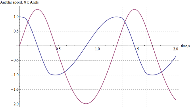
Figure 6.2. 8 times re-scaled solution (violet line) in radians and its derivative in rad/s (at $\theta=\theta_{0}=\pi/40$ rad we can see a corner point). Parameters used: $L_{1}=0.4\text{ m}$, $L_{2}=0.2\text{ m}$, $g=9.8\text{ m/$\text{s}^{2}$}$.

In Figure 6.3, we show the second derivative graph. Directly from (6.9) and (6.7) we can prove that when $\theta(t)=\theta_{0}$, $\ddot{\theta}(t)$ is an infinite number and hence $\dot{\theta}(t)$ has a corner point. Because of the classical Mathematica implementation of $H$ and $\delta$ we can say that these graphs represent the solution far from the singularities.

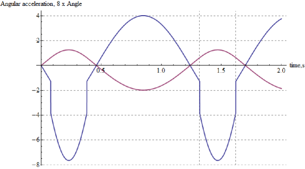
Figure 6.3. 8 times re-scaled solution in radians (violet line) and its second derivative in rad/$\text{s}^{2}$

6.2. Oscillations damped by two media

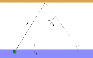
Figure 6.4. Simple pendulum moving in two media

The second example concerns oscillations of a pendulum in the interface of two media. Since we are not interested at the dynamics occurring at singular times (i.e. at the changing of the medium), this can be considered only a toy model approximating the case of a very small but sufficiently heavy moving particle.

We hence want to model the system employing a “jump” in the damping coefficient $\beta$, i.e. a finite change occurring in an infinitesimal interval of time, see Fig. 6.4. Since the frictional forces acting in this case are not conservative, it is well-known that the Euler-Lagrange equations cannot be assumed to describe the dynamics of the system and we have to use the D’Alembert principle, see [23] for details.

The kinetic energy is given by:

$$T(\dot{\theta})=\frac{1}{2}m\dot{\theta}^{2}\Lambda^{2},$$ (6.16)

and the potential energy (the zero level is the suspension point of the pendulum) is:

$$U(\theta)=-mg\Lambda\cos\theta.$$ (6.17)

In case of fluid resistance proportional to the velocity, we can introduce the generalized forces $Q$ as:

$$Q(\dot{\theta})=-r\Lambda^{2}\dot{\theta},$$ (6.18)

where $r$ is a proportional coefficient depending on the media. Let’s define the Lagrangian $L$ as

$$L(\theta,\dot{\theta}):=T(\dot{\theta})-U(\theta).$$ (6.19)

We hence assume that the equation of motion for this non-conservative system is given by the D’Alembert’s principle, i.e.

$$\frac{\mathchoice{\hbox{\rm d}}{\hbox{\rm d}}{\scalebox{0.75}{$\hbox{\rm d}$}}{\scalebox{0.35}{$\hbox{\rm d}$}}}{\mathchoice{\hbox{\rm d}t}{\hbox{\rm d}t}{\scalebox{0.75}{$\hbox{\rm d}t$}}{\scalebox{0.35}{$\hbox{\rm d}t$}}}\frac{\partial L}{\partial\dot{\theta}}-\frac{\partial L}{\partial\theta}=Q.$$ (6.20)

Inserting (6.16), (6.17) and (6.18) into (6.20) we obtain the following equation of motion:

$$m\Lambda^{2}\ddot{\theta}+mg\Lambda\sin\theta=-r\Lambda^{2}\dot{\theta}.$$ (6.21)

By introducing the damping coefficient $\beta(\theta):=r(\theta)/(2m)$ (we clearly assume that the mass $m\in\mathchoice{{\vphantom{\mathbb{R}}}^{\scalebox{0.6}{$\rho$}}}{{\vphantom{\mathbb{R}}}^{\scalebox{0.56}{$\rho$}}}{{\vphantom{\mathbb{R}}}^{\scalebox{0.47}{$\rho$}}}{{\vphantom{\mathbb{R}}}^{\scalebox{0.35}{$\rho$}}}\widetilde{\mathbb{R}}>0$ is invertible) we obtain the classical form of the equation of motion for damped oscillations:

$$\ddot{\theta}+2\beta(\theta)\dot{\theta}+\frac{g\sin\theta}{\Lambda}=0.$$ (6.22)

If the pendulum crosses the boundary between two media with damping coefficients $\beta_{1}$ and $\beta_{2}$, we can model the system using the Heaviside function $H$:

$$\beta(\theta)=\beta_{1}+\left(H(\theta+\theta_{0})-H(\theta-\theta_{0})\right)(\beta_{2}-\beta_{1}),$$ (6.23)

where $\theta=\pm\theta_{0}$ are the angles at which we have the changing of the medium (singularities).

The numerical solution of (6.22) with $\beta$ defined by (6.23) and initial conditions (6.15) is presented in Fig. 6.5. The numerical solution has been computed using Mathematica Solver NDSolve, but with an implementation of the Heaviside’s function $H$ corresponding to Thm. 18, i.e. as represented in Fig. 3.1.

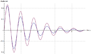
Figure 6.5. Solution $\theta$ of (6.22) (blue line). For comparison, the violet line is the case $\beta=\text{const}.=\beta_{1}$. Used parameters: $\beta_{1}=0.0064$ (air), $\beta_{2}=0.3859$ (water), $\theta_{0}=\pi/40\text{ rad}$, $\Lambda=0.6\text{ m}$, $g=9.8\text{ m/$\text{s}^{2}$}$.

We also include the graphs of the angular frequency $\dot{\theta}$ (which shows corner points) and of the angular acceleration $\ddot{\theta}$ (which shows “jumps”, i.e. infinite derivatives at singular times, as we can directly see from (6.22) and (6.23)).

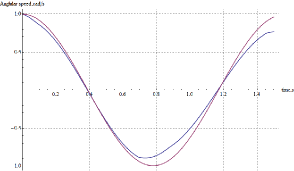
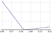
Figure 6.6. First derivative $\dot{\theta}$ of the solution of (6.22) (blue line). The case with $\beta=\text{const}=\beta_{1}$ is also shown for comparison (violet line). Note the corner points at the singular moments, for example at $t=0.083\text{ s}$ (scaled in the right figure).

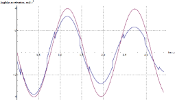
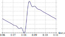
Figure 6.7. Second derivative $\ddot{\theta}$ of the solution of (6.22) (blue line). The case with $\beta=\text{const}=\beta_{1}$ is also shown for comparison (violet line). Note the “jumps” at the singular moments, for example at $t=0.083\text{ s}$ (scaled in the right figure). The infinitesimal oscillations are caused by the embedding as GSF of the Heaviside function.

6.3. Non linear strain-stress model

In this section, we want to show how to construct a mathematical model starting from an empirical function (the strain-stress relation for a steel sample) and representing it as a GSF. Starting from Newton’s second law, we hence arrive at a single nonlinear equation describing the behaviour of the steel sample. Since the empirical function is not differentiable at the end of the linear part, the use of GSF is therefore essential.

The strain-stress curve we consider is shown in Fig. 6.8.

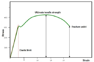
Figure 6.8. Strain-stress empirical model of the steel (see [61]).

We recall that stress can be defined as $\sigma=\frac{F}{S_{0}}$, where $F$ is the force applied to the sample, and $S_{0}$ is the initial cross-section of the cylindrical sample. The strain $\varepsilon$ is usually introduced as $\varepsilon=\frac{L-L_{0}}{L_{0}}$, where $L_{0}$ is the unstressed length and $L$ is the length after force application. In order to reproduce the experimental dependence of Fig. 6.8 we considered the parameters $d=0.37\,$mm for the diameter of the steel cilinder, and $L_{0}=2.2\,$m for the unstressed length of the sample. Thus, during the elastic behaviour (linear part) we have a Young’s modulus $E=\frac{\sigma}{\varepsilon}=2.13\cdot 10^{11}\,\text{Pa}$, a stiffness $k=\frac{ES_{0}}{L_{0}}=10423\,\frac{\text{N}}{\text{m}}$, and hence the magnitude of the linear part of the force is given by $F_{\text{l}}(x)=kx$. For the nonlinear part of the empirical law, we use the Mathematica built-in function NonlinearModelFit, see [80]. The result is shown in Fig. 6.9.

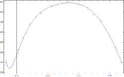
Figure 6.9. Non-linear part modelling of the strain-stress curve using the NonlinearModelFit. The dots are values extracted from the original data.

The resulting expression is

$$F_{\text{n}}(x)=a_{1}\exp(a_{2}x)+a_{3}\cos(a_{4}x)+a_{5}x+a_{6}x^{2}+a_{7}x^{3}+a_{8}x^{4}+a_{9}x^{5}+a_{10}x^{6}+a_{11}x^{7},$$ (6.24)

where the coefficients $a_{k}$ are given in Tab. 1.

$a_{1}=1.5\cdot 10^{3}$	$a_{5}=-9.9\cdot 10^{4}$	$a_{9}=-1.8\cdot 10^{9}$
$a_{2}=3.9$	$a_{6}=2.8\cdot 10^{6}$	$a_{10}=4.8\cdot 10^{9}$
$a_{3}=3.0$	$a_{7}=-4.4\cdot 10^{7}$	$a_{11}=-5.1\cdot 10^{9}$
$a_{4}=1.0\cdot 10^{2}$	$a_{8}=3.8\cdot 10^{8}$

Table 1. Coefficients used in non-linear part $F_{\text{n}}$ of the force.

Using the Heaviside function, we can hence write the force $F$ acting on the steel sample as

$$F(x)=-F_{\text{l}}(x)-(F_{\text{n}}(x)-F_{\text{l}}(x))H(x-x_{0}),$$ (6.25)

and it is represented in Fig. 6.10. Note that the negative sign is due to the fact that the force is directed opposite to the elongation of the sample; moreover, $x_{0}=0.033$ according to Fig. 6.10. Thus, the position $x$ of the steel sample satisfies the differential equation

$$\ddot{x}-\frac{F(x)}{m}=0.$$ (6.26)

Once again, note that the GSF $F$ is nonlinear and the term $F(x(t))$ is a composition of GSF.

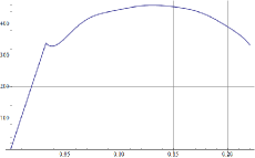
Figure 6.10. Recomputed strain-stress model.

Far from the singularity $x=x_{0}$, the validity of (6.26) can also be seen using the conservation of the mechanical energy. In fact, if $x$ is far from $x_{0}$, in the sense that $x\leq x_{1}$ for some $x_{1}\in\mathbb{R}_{<0}$, then $F(x)=-F_{\text{l}}(x)$ and we are in the zone of Hooke’s law; we thus have the potential energy: $U(x)=\frac{kx^{2}}{2}$. Similarly, if $x\geq x_{2}$ for some $x_{2}\in\mathbb{R}_{>0}$, then $F(x)=-F_{\text{n}}(x)$ and $U(x)=\frac{a_{1}}{a_{2}}\exp(a_{2}x)+\frac{a_{3}}{a_{4}}\sin(a_{4}x)+\frac{a_{5}}{2}x^{2}+\frac{a_{6}}{3}x^{3}+\frac{a_{7}}{4}x^{4}+\frac{a_{8}}{5}x^{5}+\frac{a_{9}}{6}x^{6}+\frac{a_{10}}{7}x^{7}+\frac{a_{11}}{8}x^{8}$. Therefore, far from the singularity, the conservation of the mechanical energy is equivalent to (6.26).

Clearly, the nonlinear behaviour depends on the initial conditions: if $x(0)=0.0\,\text{m}$ and $\dot{x}(0)=5\,\frac{\text{m}}{\text{s}}$, we remain in the linear setting, whereas for $x(0)=0.0\,\text{m}$, $\dot{x}(0)=15\,\frac{\text{m}}{\text{s}}$ we enter into the nonlinear one, see Fig. 6.11.

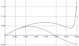
Figure 6.11. The solution $x(t)$ of equation 6.26 with initial conditions $x(0)=0.0\,\text{m},$$\dot{x}(0)=15\,\frac{\text{m}}{\text{s}}$ (blue line) in comparison with the solution in the linear setting for $x(0)=0.0\,\text{m}$, $\dot{x}(0)=5\,\frac{\text{m}}{\text{s}}$ (violet line).

See also [13, 63, 64, 65] for more complete models of this type in the setting of Colombeau theory.

6.4. Discontinuous Lagrangians in optics (Snell’s law derivation)

A typical example where one would like to use the usual results of calculus despite dealing with non differentiable functions, is geometrical optics at the interface of two media, where usually the Lagrangian function is not smooth. It is well-know, e.g., that the rigorous derivation of Snell’s law is a paradigmatic example, see e.g. [77]. The main aim of this section is to show the features of the nonlinear calculus of GSF by deriving Snell’s law for plane stratified media from the classical Fermat’s principle. For example, in the following deduction, the refraction index $n(x)$ can be any GSF, e.g. the embedding of a locally integrable function. For more general versions of Snell’s law in different media, see e.g. [12, 67]. For the classical deduction where the refraction index $n(x)$ and the light path $x=x(s)$ are $\mathcal{C}^{2}$ functions, see e.g. [46, 60].

We assume that we are considering a body $B:=\langle B_{\varepsilon}\rangle\subseteq\mathbb{R}^{3}$ represented by the strongly internal set generated by the net $B_{\varepsilon}\subseteq\mathbb{R}^{3}$, and that our light path satisfies the classical Fermat principle, i.e. the path of light between two given points $P$, $Q\in B$ is the one which minimizes the travel time. In order to mathematically state this principle for GSF, we introduce the space of paths (see [49, 23] for details):

$$\mathchoice{{\vphantom{\mathcal{G}}}^{\scalebox{0.6}{$\rho$}}}{{\vphantom{\mathcal{G}}}^{\scalebox{0.56}{$\rho$}}}{{\vphantom{\mathcal{G}}}^{\scalebox{0.47}{$\rho$}}}{{\vphantom{\mathcal{G}}}^{\scalebox{0.35}{$\rho$}}}\mathcal{GC}^{\infty}_{\text{bd}}(P,Q):=\left\{r\in\mathchoice{{\vphantom{\mathcal{G}}}^{\scalebox{0.6}{$\rho$}}}{{\vphantom{\mathcal{G}}}^{\scalebox{0.56}{$\rho$}}}{{\vphantom{\mathcal{G}}}^{\scalebox{0.47}{$\rho$}}}{{\vphantom{\mathcal{G}}}^{\scalebox{0.35}{$\rho$}}}\mathcal{GC}^{\infty}([0,1],B)\mid r(0)=P,\ r(1)=Q\right\},$$ (6.27)

and the travel time functional

$$T[r]:=\frac{1}{c}\int_{0}^{1}n(r)\,\mathchoice{\hbox{\rm d}r}{\hbox{\rm d}r}{\scalebox{0.75}{$\hbox{\rm d}r$}}{\scalebox{0.35}{$\hbox{\rm d}r$}}:=\frac{1}{c}\int_{0}^{1}n(r(s))\left|\dot{r}(s)\right|\,\mathchoice{\hbox{\rm d}s}{\hbox{\rm d}s}{\scalebox{0.75}{$\hbox{\rm d}s$}}{\scalebox{0.35}{$\hbox{\rm d}s$}}\quad\forall r\in\mathchoice{{\vphantom{\mathcal{G}}}^{\scalebox{0.6}{$\rho$}}}{{\vphantom{\mathcal{G}}}^{\scalebox{0.56}{$\rho$}}}{{\vphantom{\mathcal{G}}}^{\scalebox{0.47}{$\rho$}}}{{\vphantom{\mathcal{G}}}^{\scalebox{0.35}{$\rho$}}}\mathcal{GC}^{\infty}_{\text{bd}}(P,Q).$$ (6.28)

As usual, $c$ is the speed of light in vacuum, and $n\in\mathchoice{{\vphantom{\mathcal{G}}}^{\scalebox{0.6}{$\rho$}}}{{\vphantom{\mathcal{G}}}^{\scalebox{0.56}{$\rho$}}}{{\vphantom{\mathcal{G}}}^{\scalebox{0.47}{$\rho$}}}{{\vphantom{\mathcal{G}}}^{\scalebox{0.35}{$\rho$}}}\mathcal{GC}^{\infty}(B,\mathchoice{{\vphantom{\mathbb{R}}}^{\scalebox{0.6}{$\rho$}}}{{\vphantom{\mathbb{R}}}^{\scalebox{0.56}{$\rho$}}}{{\vphantom{\mathbb{R}}}^{\scalebox{0.47}{$\rho$}}}{{\vphantom{\mathbb{R}}}^{\scalebox{0.35}{$\rho$}}}\widetilde{\mathbb{R}}_{\geq 0})$ is the refraction index of the media $B$ we are considering. The Fermat principle hence implies that the light path $r\in\mathchoice{{\vphantom{\mathcal{G}}}^{\scalebox{0.6}{$\rho$}}}{{\vphantom{\mathcal{G}}}^{\scalebox{0.56}{$\rho$}}}{{\vphantom{\mathcal{G}}}^{\scalebox{0.47}{$\rho$}}}{{\vphantom{\mathcal{G}}}^{\scalebox{0.35}{$\rho$}}}\mathcal{GC}^{\infty}_{\text{bd}}(P,Q)$ is a weak extremal of the travel time functional $T[-]$, i.e. it satisfies

$$\delta T(r;h):=\left.\frac{\mathchoice{\hbox{\rm d}}{\hbox{\rm d}}{\scalebox{0.75}{$\hbox{\rm d}$}}{\scalebox{0.35}{$\hbox{\rm d}$}}}{\mathchoice{\hbox{\rm d}x}{\hbox{\rm d}x}{\scalebox{0.75}{$\hbox{\rm d}x$}}{\scalebox{0.35}{$\hbox{\rm d}x$}}}T[r+xh]\right|_{x=0}=0\quad\forall h\in\mathchoice{{\vphantom{\mathcal{G}}}^{\scalebox{0.6}{$\rho$}}}{{\vphantom{\mathcal{G}}}^{\scalebox{0.56}{$\rho$}}}{{\vphantom{\mathcal{G}}}^{\scalebox{0.47}{$\rho$}}}{{\vphantom{\mathcal{G}}}^{\scalebox{0.35}{$\rho$}}}\mathcal{GC}^{\infty}_{\text{bd}}(0,0).$$ (6.29)

Note that, since in (6.27) we consider only paths $r\in\mathchoice{{\vphantom{\mathcal{G}}}^{\scalebox{0.6}{$\rho$}}}{{\vphantom{\mathcal{G}}}^{\scalebox{0.56}{$\rho$}}}{{\vphantom{\mathcal{G}}}^{\scalebox{0.47}{$\rho$}}}{{\vphantom{\mathcal{G}}}^{\scalebox{0.35}{$\rho$}}}\mathcal{GC}^{\infty}([0,1],B)$ valued in the strongly internal set $B=\langle B_{\varepsilon}\rangle$, Thm. 11 implies

$$\forall h\in\mathchoice{{\vphantom{\mathcal{G}}}^{\scalebox{0.6}{$\rho$}}}{{\vphantom{\mathcal{G}}}^{\scalebox{0.56}{$\rho$}}}{{\vphantom{\mathcal{G}}}^{\scalebox{0.47}{$\rho$}}}{{\vphantom{\mathcal{G}}}^{\scalebox{0.35}{$\rho$}}}\mathcal{GC}^{\infty}_{\text{bd}}(0,0)\,\exists\delta\in\mathchoice{{\vphantom{\mathbb{R}}}^{\scalebox{0.6}{$\rho$}}}{{\vphantom{\mathbb{R}}}^{\scalebox{0.56}{$\rho$}}}{{\vphantom{\mathbb{R}}}^{\scalebox{0.47}{$\rho$}}}{{\vphantom{\mathbb{R}}}^{\scalebox{0.35}{$\rho$}}}\widetilde{\mathbb{R}}_{>0}\,\forall x\in(-\delta,\delta):\ r+xh\in\mathchoice{{\vphantom{\mathcal{G}}}^{\scalebox{0.6}{$\rho$}}}{{\vphantom{\mathcal{G}}}^{\scalebox{0.56}{$\rho$}}}{{\vphantom{\mathcal{G}}}^{\scalebox{0.47}{$\rho$}}}{{\vphantom{\mathcal{G}}}^{\scalebox{0.35}{$\rho$}}}\mathcal{GC}^{\infty}([0,1],B),$$

and therefore, it is correct to consider the derivative in (6.29). Physically this means that we are considering only paths which lay completely inside the body $B=\langle B_{\varepsilon}\rangle$. The weak extremal condition (6.29) is equivalent to the Euler-Lagrange equations (see [49]) for the Lagrangian $(r,v)\mapsto L(r,v):=n(r)\sqrt{v\cdot v}\in\mathchoice{{\vphantom{\mathcal{G}}}^{\scalebox{0.6}{$\rho$}}}{{\vphantom{\mathcal{G}}}^{\scalebox{0.56}{$\rho$}}}{{\vphantom{\mathcal{G}}}^{\scalebox{0.47}{$\rho$}}}{{\vphantom{\mathcal{G}}}^{\scalebox{0.35}{$\rho$}}}\mathcal{GC}^{\infty}(B\times\mathchoice{{\vphantom{\mathbb{R}}}^{\scalebox{0.6}{$\rho$}}}{{\vphantom{\mathbb{R}}}^{\scalebox{0.56}{$\rho$}}}{{\vphantom{\mathbb{R}}}^{\scalebox{0.47}{$\rho$}}}{{\vphantom{\mathbb{R}}}^{\scalebox{0.35}{$\rho$}}}\widetilde{\mathbb{R}}^{3},\mathchoice{{\vphantom{\mathbb{R}}}^{\scalebox{0.6}{$\rho$}}}{{\vphantom{\mathbb{R}}}^{\scalebox{0.56}{$\rho$}}}{{\vphantom{\mathbb{R}}}^{\scalebox{0.47}{$\rho$}}}{{\vphantom{\mathbb{R}}}^{\scalebox{0.35}{$\rho$}}}\widetilde{\mathbb{R}})$. We use the notation $L(r,v)=L(r_{1},r_{2},r_{3},v_{1},v_{2},v_{3})$ for the variables of $L$. We also explicitly note the nonlinear operations in this Lagrangian, and the composition $n(r(s))$ of GSF. We use the customary notations $\vec{v}(s):=\frac{\mathchoice{\hbox{\rm d}r}{\hbox{\rm d}r}{\scalebox{0.75}{$\hbox{\rm d}r$}}{\scalebox{0.35}{$\hbox{\rm d}r$}}}{\mathchoice{\hbox{\rm d}s}{\hbox{\rm d}s}{\scalebox{0.75}{$\hbox{\rm d}s$}}{\scalebox{0.35}{$\hbox{\rm d}s$}}}(s)\in\mathchoice{{\vphantom{\mathbb{R}}}^{\scalebox{0.6}{$\rho$}}}{{\vphantom{\mathbb{R}}}^{\scalebox{0.56}{$\rho$}}}{{\vphantom{\mathbb{R}}}^{\scalebox{0.47}{$\rho$}}}{{\vphantom{\mathbb{R}}}^{\scalebox{0.35}{$\rho$}}}\widetilde{\mathbb{R}}^{3}$, $v(s):=|\vec{v}(s)|\in\mathchoice{{\vphantom{\mathbb{R}}}^{\scalebox{0.6}{$\rho$}}}{{\vphantom{\mathbb{R}}}^{\scalebox{0.56}{$\rho$}}}{{\vphantom{\mathbb{R}}}^{\scalebox{0.47}{$\rho$}}}{{\vphantom{\mathbb{R}}}^{\scalebox{0.35}{$\rho$}}}\widetilde{\mathbb{R}}$, and $L[r](s):=L(r(s),\vec{v}(s))$. We hence get

$$\frac{\mathchoice{\hbox{\rm d}}{\hbox{\rm d}}{\scalebox{0.75}{$\hbox{\rm d}$}}{\scalebox{0.35}{$\hbox{\rm d}$}}}{\mathchoice{\hbox{\rm d}s}{\hbox{\rm d}s}{\scalebox{0.75}{$\hbox{\rm d}s$}}{\scalebox{0.35}{$\hbox{\rm d}s$}}}\left(\frac{\partial L}{\partial v_{j}}[r](s)\right)=\frac{\partial L}{\partial r_{j}}[r](s),\quad\forall j=1,2,3,\ \forall s\in[0,1].$$ (6.30)

We always assume that the frame of reference is chosen so that the light path satisfies $v(s)\in\mathchoice{{\vphantom{\mathbb{R}}}^{\scalebox{0.6}{$\rho$}}}{{\vphantom{\mathbb{R}}}^{\scalebox{0.56}{$\rho$}}}{{\vphantom{\mathbb{R}}}^{\scalebox{0.47}{$\rho$}}}{{\vphantom{\mathbb{R}}}^{\scalebox{0.35}{$\rho$}}}\widetilde{\mathbb{R}}_{>0}$. Calculating the derivatives $\partial L/\partial v_{j}$ and $\partial L/\partial r_{j}$ in Euler-Lagrange equations, we get

$$\frac{\partial L}{\partial v_{j}}(r,v) =n(r)\frac{v_{j}}{\sqrt{v\cdot v}}$$

$$\frac{\partial L}{\partial r_{j}}(r,v) =\frac{\partial n}{\partial r_{j}}(r)\sqrt{v\cdot v},$$

for all $(r,v)\in B\times\mathchoice{{\vphantom{\mathbb{R}}}^{\scalebox{0.6}{$\rho$}}}{{\vphantom{\mathbb{R}}}^{\scalebox{0.56}{$\rho$}}}{{\vphantom{\mathbb{R}}}^{\scalebox{0.47}{$\rho$}}}{{\vphantom{\mathbb{R}}}^{\scalebox{0.35}{$\rho$}}}\widetilde{\mathbb{R}}^{3}$ and all $j=1,2,3$. Substituting in (6.30), we obtain the eikonal equation

$$\frac{\mathchoice{\hbox{\rm d}}{\hbox{\rm d}}{\scalebox{0.75}{$\hbox{\rm d}$}}{\scalebox{0.35}{$\hbox{\rm d}$}}}{\mathchoice{\hbox{\rm d}s}{\hbox{\rm d}s}{\scalebox{0.75}{$\hbox{\rm d}s$}}{\scalebox{0.35}{$\hbox{\rm d}s$}}}\left(n(r(s))\frac{\vec{v}(s)}{v(s)}\right)=\nabla n(r(s))v(s),\quad\forall s\in[0,1].$$ (6.31)

We now consider the case of a plane stratified media, i.e. where $n$ changes only along one direction $\vec{k}\in\mathchoice{{\vphantom{\mathbb{R}}}^{\scalebox{0.6}{$\rho$}}}{{\vphantom{\mathbb{R}}}^{\scalebox{0.56}{$\rho$}}}{{\vphantom{\mathbb{R}}}^{\scalebox{0.47}{$\rho$}}}{{\vphantom{\mathbb{R}}}^{\scalebox{0.35}{$\rho$}}}\widetilde{\mathbb{R}}^{3}$, $|\vec{k}|=1$, so that

$$\nabla n(r(s))\parallel\vec{k}\quad\forall s\in[0,1].$$ (6.32)

For simplicity, where it is clear, we omit the evaluation at $s$. Thus, the cross product of the two vectors $\nabla n(r)$ and $\vec{k}$ is $\vec{k}\times\nabla n(r)=0=\vec{k}\times\nabla n(r)v$. Using (6.31) we get $\vec{k}\times\frac{\mathchoice{\hbox{\rm d}}{\hbox{\rm d}}{\scalebox{0.75}{$\hbox{\rm d}$}}{\scalebox{0.35}{$\hbox{\rm d}$}}}{\mathchoice{\hbox{\rm d}s}{\hbox{\rm d}s}{\scalebox{0.75}{$\hbox{\rm d}s$}}{\scalebox{0.35}{$\hbox{\rm d}s$}}}(n(r)\frac{\vec{v}}{v})=0$, and hence $\frac{\mathchoice{\hbox{\rm d}}{\hbox{\rm d}}{\scalebox{0.75}{$\hbox{\rm d}$}}{\scalebox{0.35}{$\hbox{\rm d}$}}}{\mathchoice{\hbox{\rm d}s}{\hbox{\rm d}s}{\scalebox{0.75}{$\hbox{\rm d}s$}}{\scalebox{0.35}{$\hbox{\rm d}s$}}}(\vec{k}\times n(r(s))\frac{\vec{v}(s)}{v(s)})=0$ for all $s\in[0,1]$, i.e. the function $s\in[0,1]\mapsto\vec{k}\times n(r(s))\frac{\vec{v}(s)}{v(s)}\in\mathchoice{{\vphantom{\mathbb{R}}}^{\scalebox{0.6}{$\rho$}}}{{\vphantom{\mathbb{R}}}^{\scalebox{0.56}{$\rho$}}}{{\vphantom{\mathbb{R}}}^{\scalebox{0.47}{$\rho$}}}{{\vphantom{\mathbb{R}}}^{\scalebox{0.35}{$\rho$}}}\widetilde{\mathbb{R}}^{3}$ is a constant $\vec{C}\in\mathchoice{{\vphantom{\mathbb{R}}}^{\scalebox{0.6}{$\rho$}}}{{\vphantom{\mathbb{R}}}^{\scalebox{0.56}{$\rho$}}}{{\vphantom{\mathbb{R}}}^{\scalebox{0.47}{$\rho$}}}{{\vphantom{\mathbb{R}}}^{\scalebox{0.35}{$\rho$}}}\widetilde{\mathbb{R}}^{3}$. Taking its magnitude $C=|\vec{C}|$

$$\forall s\in[0,1]:\ C=|\vec{k}|\left|n(r(s))\right|\left|\frac{\vec{v}(s)}{v(s)}\right|\sin\varphi(s),$$

where $\varphi(s)$ is the angle between $\vec{k}$ and $\vec{v}(s)=\frac{\mathchoice{\hbox{\rm d}r}{\hbox{\rm d}r}{\scalebox{0.75}{$\hbox{\rm d}r$}}{\scalebox{0.35}{$\hbox{\rm d}r$}}}{\mathchoice{\hbox{\rm d}s}{\hbox{\rm d}s}{\scalebox{0.75}{$\hbox{\rm d}s$}}{\scalebox{0.35}{$\hbox{\rm d}s$}}}(s)$. We proved Snell’s law for GSF:

Theorem 58.

Let $B_{\varepsilon}\subseteq\mathbb{R}^{3}$, $B:=\langle B_{\varepsilon}\rangle$, $P$, $Q\in\langle B_{\varepsilon}\rangle$, $n\in\mathchoice{{\vphantom{\mathcal{G}}}^{\scalebox{0.6}{$\rho$}}}{{\vphantom{\mathcal{G}}}^{\scalebox{0.56}{$\rho$}}}{{\vphantom{\mathcal{G}}}^{\scalebox{0.47}{$\rho$}}}{{\vphantom{\mathcal{G}}}^{\scalebox{0.35}{$\rho$}}}\mathcal{GC}^{\infty}(B,\mathchoice{{\vphantom{\mathbb{R}}}^{\scalebox{0.6}{$\rho$}}}{{\vphantom{\mathbb{R}}}^{\scalebox{0.56}{$\rho$}}}{{\vphantom{\mathbb{R}}}^{\scalebox{0.47}{$\rho$}}}{{\vphantom{\mathbb{R}}}^{\scalebox{0.35}{$\rho$}}}\widetilde{\mathbb{R}}_{\geq 0})$. Assume that $r\in\mathchoice{{\vphantom{\mathcal{G}}}^{\scalebox{0.6}{$\rho$}}}{{\vphantom{\mathcal{G}}}^{\scalebox{0.56}{$\rho$}}}{{\vphantom{\mathcal{G}}}^{\scalebox{0.47}{$\rho$}}}{{\vphantom{\mathcal{G}}}^{\scalebox{0.35}{$\rho$}}}\mathcal{GC}^{\infty}_{\text{\emph{bd}}}(P,Q)$ is a weak extremal of the travel time functional (6.28), i.e. it satisfies (6.29). Set $\vec{v}(s):=\frac{\mathchoice{\hbox{\rm d}r}{\hbox{\rm d}r}{\scalebox{0.75}{$\hbox{\rm d}r$}}{\scalebox{0.35}{$\hbox{\rm d}r$}}}{\mathchoice{\hbox{\rm d}s}{\hbox{\rm d}s}{\scalebox{0.75}{$\hbox{\rm d}s$}}{\scalebox{0.35}{$\hbox{\rm d}s$}}}(s)\in\mathchoice{{\vphantom{\mathbb{R}}}^{\scalebox{0.6}{$\rho$}}}{{\vphantom{\mathbb{R}}}^{\scalebox{0.56}{$\rho$}}}{{\vphantom{\mathbb{R}}}^{\scalebox{0.47}{$\rho$}}}{{\vphantom{\mathbb{R}}}^{\scalebox{0.35}{$\rho$}}}\widetilde{\mathbb{R}}^{3}$, $v(s):=|\vec{v}(s)|\in\mathchoice{{\vphantom{\mathbb{R}}}^{\scalebox{0.6}{$\rho$}}}{{\vphantom{\mathbb{R}}}^{\scalebox{0.56}{$\rho$}}}{{\vphantom{\mathbb{R}}}^{\scalebox{0.47}{$\rho$}}}{{\vphantom{\mathbb{R}}}^{\scalebox{0.35}{$\rho$}}}\widetilde{\mathbb{R}}$ and assume that $v(s)>0$ for all $s\in[0,1]$. Then the eikonal equation (6.31) holds. Moreover, if $\nabla n(r(s))\parallel\vec{k}$, where $\vec{k}\in\mathchoice{{\vphantom{\mathbb{R}}}^{\scalebox{0.6}{$\rho$}}}{{\vphantom{\mathbb{R}}}^{\scalebox{0.56}{$\rho$}}}{{\vphantom{\mathbb{R}}}^{\scalebox{0.47}{$\rho$}}}{{\vphantom{\mathbb{R}}}^{\scalebox{0.35}{$\rho$}}}\widetilde{\mathbb{R}}^{3}$, $|\vec{k}|=1$, and $\varphi(s)$ is the angle between $\vec{k}$ and $\vec{v}(s),$then the quantity $n(r(s))\cdot\sin\varphi(s)$ is constant for all $s\in[0,1]$.

6.5. Finite and infinite step potential

Models of quantum mechanics such as the potential well or the step potential with finite or infinite walls are clear and simple examples showing features of various quantum mechanical effects, see e.g. [11]. However, the mathematics of such models is not very clear sometimes, see again e.g. [11, pag. 34-40, pag. 68] and authors’ comments about mathematical rigour. Once again, in this section we see how the formalism of GSF theory allows one to completely recover a mathematically and physically clear proof by formalizing the intuitive steps of [11, pag. 68]. We consider the step-potential problem, where the high of the potential can be any finite or infinite generalized number; a similar approach can be used for the rectangular potential wells.

In the following, we write $x\ll 0$ if $\exists r\in\mathbb{R}_{<0}:\ x<r$, and similarly for $x\gg 0$, and we simply say that $x$ is far from $0$. The step function potential for the one-dimensional stationary Schrodinger equation is a GSF $U\in\mathchoice{{\vphantom{\mathcal{G}}}^{\scalebox{0.6}{$\rho$}}}{{\vphantom{\mathcal{G}}}^{\scalebox{0.56}{$\rho$}}}{{\vphantom{\mathcal{G}}}^{\scalebox{0.47}{$\rho$}}}{{\vphantom{\mathcal{G}}}^{\scalebox{0.35}{$\rho$}}}\mathcal{GC}^{\infty}(\mathchoice{{\vphantom{\mathbb{R}}}^{\scalebox{0.6}{$\rho$}}}{{\vphantom{\mathbb{R}}}^{\scalebox{0.56}{$\rho$}}}{{\vphantom{\mathbb{R}}}^{\scalebox{0.47}{$\rho$}}}{{\vphantom{\mathbb{R}}}^{\scalebox{0.35}{$\rho$}}}\widetilde{\mathbb{R}},\mathchoice{{\vphantom{\mathbb{R}}}^{\scalebox{0.6}{$\rho$}}}{{\vphantom{\mathbb{R}}}^{\scalebox{0.56}{$\rho$}}}{{\vphantom{\mathbb{R}}}^{\scalebox{0.47}{$\rho$}}}{{\vphantom{\mathbb{R}}}^{\scalebox{0.35}{$\rho$}}}\widetilde{\mathbb{R}})$ such that

$$U(x)=\begin{cases}0&x\ll 0,\\ U_{0}&x\gg 0,\end{cases}$$ (6.33)

where $U_{0}\in\mathchoice{{\vphantom{\mathbb{R}}}^{\scalebox{0.6}{$\rho$}}}{{\vphantom{\mathbb{R}}}^{\scalebox{0.56}{$\rho$}}}{{\vphantom{\mathbb{R}}}^{\scalebox{0.47}{$\rho$}}}{{\vphantom{\mathbb{R}}}^{\scalebox{0.35}{$\rho$}}}\widetilde{\mathbb{R}}_{>0}$ is an arbitrary generalized number (finite or infinite). For example, $U(x)=H(x)\cdot U_{0}$ satisfies these conditions. However, as stated in [11, pag. 34], this is actually an idealized model of the potential, and we cannot say it is a physically meaningful model for infinitesimal $x\approx 0$ (similarly to what we have already seen e.g. in Sec. 6.1 for the singular variable length pendulum).

The system satisfies the stationary Schrodinger’s equation

$$\left[-\frac{\hbar^{2}}{2m}\frac{\mathchoice{\hbox{\rm d}}{\hbox{\rm d}}{\scalebox{0.75}{$\hbox{\rm d}$}}{\scalebox{0.35}{$\hbox{\rm d}$}}^{2}}{\mathchoice{\hbox{\rm d}x}{\hbox{\rm d}x}{\scalebox{0.75}{$\hbox{\rm d}x$}}{\scalebox{0.35}{$\hbox{\rm d}x$}}^{2}}+U(x)\right]\psi(x)=E\psi(x),$$ (6.34)

where $\hbar$ is the Planck’s constant, $m\in\mathbb{R}_{>0}$ the mass of the particle, $E$ the energy, and $\psi(x)$ the wave function. Using Thm. 52, we can state that there exists a $\psi\in\mathchoice{{\vphantom{\mathcal{G}}}^{\scalebox{0.6}{$\rho$}}}{{\vphantom{\mathcal{G}}}^{\scalebox{0.56}{$\rho$}}}{{\vphantom{\mathcal{G}}}^{\scalebox{0.47}{$\rho$}}}{{\vphantom{\mathcal{G}}}^{\scalebox{0.35}{$\rho$}}}\mathcal{GC}^{\infty}(\mathchoice{{\vphantom{\mathbb{R}}}^{\scalebox{0.6}{$\rho$}}}{{\vphantom{\mathbb{R}}}^{\scalebox{0.56}{$\rho$}}}{{\vphantom{\mathbb{R}}}^{\scalebox{0.47}{$\rho$}}}{{\vphantom{\mathbb{R}}}^{\scalebox{0.35}{$\rho$}}}\widetilde{\mathbb{R}},\mathchoice{{\vphantom{\mathbb{R}}}^{\scalebox{0.6}{$\rho$}}}{{\vphantom{\mathbb{R}}}^{\scalebox{0.56}{$\rho$}}}{{\vphantom{\mathbb{R}}}^{\scalebox{0.47}{$\rho$}}}{{\vphantom{\mathbb{R}}}^{\scalebox{0.35}{$\rho$}}}\widetilde{\mathbb{R}})$ satisfying (6.34). Repeating exactly the usual calculations, for $x\ll 0$ we have:

$$\psi(x)=\frac{1}{\sqrt{k_{1}}}\left(A_{1}e^{ik_{1}x}+A_{2}e^{-ik_{1}x}\right),$$ (6.35)

where $k_{1}:=\sqrt{2mE/\hbar^{2}}$ and $A_{1}$, $A_{2}\in\mathchoice{{\vphantom{\mathbb{R}}}^{\scalebox{0.6}{$\rho$}}}{{\vphantom{\mathbb{R}}}^{\scalebox{0.56}{$\rho$}}}{{\vphantom{\mathbb{R}}}^{\scalebox{0.47}{$\rho$}}}{{\vphantom{\mathbb{R}}}^{\scalebox{0.35}{$\rho$}}}\widetilde{\mathbb{R}}$ are undefined constants. For $x\gg 0$, we have:

$$\psi(x)=\frac{1}{\sqrt{k_{2}}}\left(B_{1}e^{ik_{2}x}+B_{2}e^{-ik_{2}x}\right),$$ (6.36)

where $k_{2}=\sqrt{2m(E-V_{0})/\hbar^{2}},$ $B_{1}$, $B_{2}\in\mathchoice{{\vphantom{\mathbb{R}}}^{\scalebox{0.6}{$\rho$}}}{{\vphantom{\mathbb{R}}}^{\scalebox{0.56}{$\rho$}}}{{\vphantom{\mathbb{R}}}^{\scalebox{0.47}{$\rho$}}}{{\vphantom{\mathbb{R}}}^{\scalebox{0.35}{$\rho$}}}\widetilde{\mathbb{R}}$ are undefined constants. As stated in [11, pag. 68], in order to find these constants, we need some mathematically careful steps to justify the corresponding initial conditions. Take any standard real number $\eta\in\mathbb{R}_{>0}$ and integrate (6.34) on $[-\eta,\eta]\subseteq\mathchoice{{\vphantom{\mathbb{R}}}^{\scalebox{0.6}{$\rho$}}}{{\vphantom{\mathbb{R}}}^{\scalebox{0.56}{$\rho$}}}{{\vphantom{\mathbb{R}}}^{\scalebox{0.47}{$\rho$}}}{{\vphantom{\mathbb{R}}}^{\scalebox{0.35}{$\rho$}}}\widetilde{\mathbb{R}}$ to get

$$\frac{\mathchoice{\hbox{\rm d}\psi}{\hbox{\rm d}\psi}{\scalebox{0.75}{$\hbox{\rm d}\psi$}}{\scalebox{0.35}{$\hbox{\rm d}\psi$}}}{\mathchoice{\hbox{\rm d}x}{\hbox{\rm d}x}{\scalebox{0.75}{$\hbox{\rm d}x$}}{\scalebox{0.35}{$\hbox{\rm d}x$}}}(\eta)-\frac{\mathchoice{\hbox{\rm d}\psi}{\hbox{\rm d}\psi}{\scalebox{0.75}{$\hbox{\rm d}\psi$}}{\scalebox{0.35}{$\hbox{\rm d}\psi$}}}{\mathchoice{\hbox{\rm d}x}{\hbox{\rm d}x}{\scalebox{0.75}{$\hbox{\rm d}x$}}{\scalebox{0.35}{$\hbox{\rm d}x$}}}(-\eta)=\frac{2m}{\hbar^{2}}\int_{-\eta}^{\eta}\left[U(x)-E\right]\psi(x)\,\mathchoice{\hbox{\rm d}x}{\hbox{\rm d}x}{\scalebox{0.75}{$\hbox{\rm d}x$}}{\scalebox{0.35}{$\hbox{\rm d}x$}}.$$ (6.37)

As in [11, pag. 68], we assume that

$$U(x)-E\text{ is finite for all finite }x\in\mathchoice{{\vphantom{\mathbb{R}}}^{\scalebox{0.6}{$\rho$}}}{{\vphantom{\mathbb{R}}}^{\scalebox{0.56}{$\rho$}}}{{\vphantom{\mathbb{R}}}^{\scalebox{0.47}{$\rho$}}}{{\vphantom{\mathbb{R}}}^{\scalebox{0.35}{$\rho$}}}\widetilde{\mathbb{R}}$$ (6.38)

$$\frac{\mathchoice{\hbox{\rm d}\psi}{\hbox{\rm d}\psi}{\scalebox{0.75}{$\hbox{\rm d}\psi$}}{\scalebox{0.35}{$\hbox{\rm d}\psi$}}}{\mathchoice{\hbox{\rm d}x}{\hbox{\rm d}x}{\scalebox{0.75}{$\hbox{\rm d}x$}}{\scalebox{0.35}{$\hbox{\rm d}x$}}}(\eta)\text{ is finite for all }\eta\in\mathbb{R}_{>0}$$ . (6.39)

From (6.37) and the first of these assumptions, we obtain

$$\left|\frac{\mathchoice{\hbox{\rm d}\psi}{\hbox{\rm d}\psi}{\scalebox{0.75}{$\hbox{\rm d}\psi$}}{\scalebox{0.35}{$\hbox{\rm d}\psi$}}}{\mathchoice{\hbox{\rm d}x}{\hbox{\rm d}x}{\scalebox{0.75}{$\hbox{\rm d}x$}}{\scalebox{0.35}{$\hbox{\rm d}x$}}}(\eta)-\frac{\mathchoice{\hbox{\rm d}\psi}{\hbox{\rm d}\psi}{\scalebox{0.75}{$\hbox{\rm d}\psi$}}{\scalebox{0.35}{$\hbox{\rm d}\psi$}}}{\mathchoice{\hbox{\rm d}x}{\hbox{\rm d}x}{\scalebox{0.75}{$\hbox{\rm d}x$}}{\scalebox{0.35}{$\hbox{\rm d}x$}}}(-\eta)\right|\leq\frac{4m}{\hbar^{2}}\cdot C\cdot\eta$$

for some $C\in\mathbb{R}_{>0}$ (coming from (6.38)), i.e.

$$\lim_{\begin{subarray}{c}\eta\to 0^{+}\\ \eta\in\mathbb{R}_{>0}\end{subarray}}\left|\frac{\mathchoice{\hbox{\rm d}\psi}{\hbox{\rm d}\psi}{\scalebox{0.75}{$\hbox{\rm d}\psi$}}{\scalebox{0.35}{$\hbox{\rm d}\psi$}}}{\mathchoice{\hbox{\rm d}x}{\hbox{\rm d}x}{\scalebox{0.75}{$\hbox{\rm d}x$}}{\scalebox{0.35}{$\hbox{\rm d}x$}}}(\eta)-\frac{\mathchoice{\hbox{\rm d}\psi}{\hbox{\rm d}\psi}{\scalebox{0.75}{$\hbox{\rm d}\psi$}}{\scalebox{0.35}{$\hbox{\rm d}\psi$}}}{\mathchoice{\hbox{\rm d}x}{\hbox{\rm d}x}{\scalebox{0.75}{$\hbox{\rm d}x$}}{\scalebox{0.35}{$\hbox{\rm d}x$}}}(-\eta)\right|=0.$$ (6.40)

Similarly, from (6.39) and the fundamental theorem of calculus for GSF Thm. 32.(v), we have

$$\left|\psi(\eta)-\psi(0)\right|=\left|\int_{0}^{\eta}\frac{\mathchoice{\hbox{\rm d}\psi}{\hbox{\rm d}\psi}{\scalebox{0.75}{$\hbox{\rm d}\psi$}}{\scalebox{0.35}{$\hbox{\rm d}\psi$}}}{\mathchoice{\hbox{\rm d}x}{\hbox{\rm d}x}{\scalebox{0.75}{$\hbox{\rm d}x$}}{\scalebox{0.35}{$\hbox{\rm d}x$}}}(x)\,\mathchoice{\hbox{\rm d}x}{\hbox{\rm d}x}{\scalebox{0.75}{$\hbox{\rm d}x$}}{\scalebox{0.35}{$\hbox{\rm d}x$}}\right|\leq\bar{C}\cdot\eta,$$

for some $\bar{C}\in\mathbb{R}_{>0}$ (coming from (6.39)), and hence

$$\lim_{\begin{subarray}{c}\eta\to 0^{+}\\ \eta\in\mathbb{R}_{>0}\end{subarray}}\left|\psi(\eta)-\psi(0)\right|=0.$$ (6.41)

Recall that from Thm. 16.(ii) and Thm. 24 it directly follows that both $\psi(x)$ and its derivative $\frac{\mathchoice{\hbox{\rm d}\psi}{\hbox{\rm d}\psi}{\scalebox{0.75}{$\hbox{\rm d}\psi$}}{\scalebox{0.35}{$\hbox{\rm d}\psi$}}}{\mathchoice{\hbox{\rm d}x}{\hbox{\rm d}x}{\scalebox{0.75}{$\hbox{\rm d}x$}}{\scalebox{0.35}{$\hbox{\rm d}x$}}}(x)$ are GSF, and hence they are continuous in the sharp topology at each point $x\in\mathchoice{{\vphantom{\mathbb{R}}}^{\scalebox{0.6}{$\rho$}}}{{\vphantom{\mathbb{R}}}^{\scalebox{0.56}{$\rho$}}}{{\vphantom{\mathbb{R}}}^{\scalebox{0.47}{$\rho$}}}{{\vphantom{\mathbb{R}}}^{\scalebox{0.35}{$\rho$}}}\widetilde{\mathbb{R}}$. Stated explicitly at $x=0$, this means that

$$\exists\lim_{\begin{subarray}{c}x\to 0\\ x\in\,\mathchoice{{\vphantom{\mathbb{R}}}^{\scalebox{0.6}{$\rho$}}}{{\vphantom{\mathbb{R}}}^{\scalebox{0.56}{$\rho$}}}{{\vphantom{\mathbb{R}}}^{\scalebox{0.47}{$\rho$}}}{{\vphantom{\mathbb{R}}}^{\scalebox{0.35}{$\rho$}}}\widetilde{\mathbb{R}}\end{subarray}}\frac{\mathchoice{\hbox{\rm d}\psi}{\hbox{\rm d}\psi}{\scalebox{0.75}{$\hbox{\rm d}\psi$}}{\scalebox{0.35}{$\hbox{\rm d}\psi$}}}{\mathchoice{\hbox{\rm d}x}{\hbox{\rm d}x}{\scalebox{0.75}{$\hbox{\rm d}x$}}{\scalebox{0.35}{$\hbox{\rm d}x$}}}(x) =\frac{\mathchoice{\hbox{\rm d}\psi}{\hbox{\rm d}\psi}{\scalebox{0.75}{$\hbox{\rm d}\psi$}}{\scalebox{0.35}{$\hbox{\rm d}\psi$}}}{\mathchoice{\hbox{\rm d}x}{\hbox{\rm d}x}{\scalebox{0.75}{$\hbox{\rm d}x$}}{\scalebox{0.35}{$\hbox{\rm d}x$}}}(0),$$

$$\exists\lim_{\begin{subarray}{c}x\to 0\\ x\in\,\mathchoice{{\vphantom{\mathbb{R}}}^{\scalebox{0.6}{$\rho$}}}{{\vphantom{\mathbb{R}}}^{\scalebox{0.56}{$\rho$}}}{{\vphantom{\mathbb{R}}}^{\scalebox{0.47}{$\rho$}}}{{\vphantom{\mathbb{R}}}^{\scalebox{0.35}{$\rho$}}}\widetilde{\mathbb{R}}\end{subarray}}\psi(x) =\psi(0),$$

and these are different than (6.40) and (6.41), where $\eta\in\mathbb{R}_{>0}$. Indeed, balls $B_{\eta}(c)\subseteq\mathchoice{{\vphantom{\mathbb{R}}}^{\scalebox{0.6}{$\rho$}}}{{\vphantom{\mathbb{R}}}^{\scalebox{0.56}{$\rho$}}}{{\vphantom{\mathbb{R}}}^{\scalebox{0.47}{$\rho$}}}{{\vphantom{\mathbb{R}}}^{\scalebox{0.35}{$\rho$}}}\widetilde{\mathbb{R}}$, for radii $\eta\in\mathbb{R}_{>0}$, generate a different topology on $\mathchoice{{\vphantom{\mathbb{R}}}^{\scalebox{0.6}{$\rho$}}}{{\vphantom{\mathbb{R}}}^{\scalebox{0.56}{$\rho$}}}{{\vphantom{\mathbb{R}}}^{\scalebox{0.47}{$\rho$}}}{{\vphantom{\mathbb{R}}}^{\scalebox{0.35}{$\rho$}}}\widetilde{\mathbb{R}}$ (called Fermat topology, see e.g. [30, 31]). See Fig. 6.12 for an intuitive diagram of the solution $\psi$ in an infinitesimal neighborhood of $x=0$: whereas $\frac{\mathchoice{\hbox{\rm d}\psi}{\hbox{\rm d}\psi}{\scalebox{0.75}{$\hbox{\rm d}\psi$}}{\scalebox{0.35}{$\hbox{\rm d}\psi$}}}{\mathchoice{\hbox{\rm d}x}{\hbox{\rm d}x}{\scalebox{0.75}{$\hbox{\rm d}x$}}{\scalebox{0.35}{$\hbox{\rm d}x$}}}(\eta)$ is continuous for $\eta\to 0$, $\eta\in\mathbb{R}_{>0}$, it is well-known (see [11]) that the same property does not hold for the second derivative. In Fig. 6.12, the green lines represents the solution for $x\ll 0$ or $x\gg 0$, and the blue one the GSF function $\psi=[\psi_{\varepsilon}(-)]$ (we actually represented $\psi_{\varepsilon}$ for $\varepsilon$ sufficiently small); we therefore have to think as infinitesimal the differences between blue and green lines, and hence as infinite the second derivative at $x=0$.

From (6.35), (6.36) and (6.40), (6.41) we obtain that the constants are uniquely determined by the system

$$\begin{cases}\left(A_{1}+A_{2}\right)=\left(B_{1}+B_{2}\right)\\ k_{1}\left(A_{1}-A_{2}\right)=k_{2}\left(B_{1}-B_{2}\right)\end{cases}$$ (6.42)

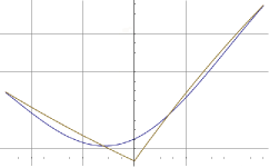
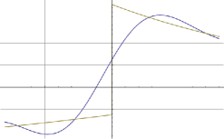
Figure 6.12. The fist derivative (left) and the second derivative (right) of the wave function $\psi$ in an infinitesimal neighborhood of $0$ (blue lines). Green lines are the same derivatives for $x\ll 0$ and $x\gg 0$.

6.6. Heisenberg uncertainty principle

We close this section of applications by mentioning how we can use infinitesimal and infinite numbers and GSF theory to fully justify the most frequent example of the Heisenberg uncertainty principle.

We do not have sufficient space here to present a complete list of result about the so called hyperfinite Fourier transform (see [59]), but we can surely present the main ideas:

1. Since in the ring $\mathchoice{{\vphantom{\mathbb{R}}}^{\scalebox{0.6}{$\rho$}}}{{\vphantom{\mathbb{R}}}^{\scalebox{0.56}{$\rho$}}}{{\vphantom{\mathbb{R}}}^{\scalebox{0.47}{$\rho$}}}{{\vphantom{\mathbb{R}}}^{\scalebox{0.35}{$\rho$}}}\widetilde{\mathbb{R}}$ we have infinite numbers $k\in\mathchoice{{\vphantom{\mathbb{R}}}^{\scalebox{0.6}{$\rho$}}}{{\vphantom{\mathbb{R}}}^{\scalebox{0.56}{$\rho$}}}{{\vphantom{\mathbb{R}}}^{\scalebox{0.47}{$\rho$}}}{{\vphantom{\mathbb{R}}}^{\scalebox{0.35}{$\rho$}}}\widetilde{\mathbb{R}}_{>0}$, e.g. $k=\mathchoice{\hbox{\rm d}\rho}{\hbox{\rm d}\rho}{\scalebox{0.75}{$\hbox{\rm d}\rho$}}{\scalebox{0.35}{$\hbox{\rm d}\rho$}}^{-1}$, and since every GSF is always integrable on a functionally compact set of the form $K:=[-k,k]^{n}\subseteq\mathchoice{{\vphantom{\mathbb{R}}}^{\scalebox{0.6}{$\rho$}}}{{\vphantom{\mathbb{R}}}^{\scalebox{0.56}{$\rho$}}}{{\vphantom{\mathbb{R}}}^{\scalebox{0.47}{$\rho$}}}{{\vphantom{\mathbb{R}}}^{\scalebox{0.35}{$\rho$}}}\widetilde{\mathbb{R}}^{n}$ (see Thm. 46), we can simply define the hyperfinite Fourier transform $\mathcal{F}_{k}\left(f\right)$ of any $f\in\mathchoice{{\vphantom{\mathcal{G}}}^{\scalebox{0.6}{$\rho$}}}{{\vphantom{\mathcal{G}}}^{\scalebox{0.56}{$\rho$}}}{{\vphantom{\mathcal{G}}}^{\scalebox{0.47}{$\rho$}}}{{\vphantom{\mathcal{G}}}^{\scalebox{0.35}{$\rho$}}}\mathcal{GC}^{\infty}(K,\mathchoice{{\vphantom{\mathbb{C}}}^{\scalebox{0.6}{$\rho$}}}{{\vphantom{\mathbb{C}}}^{\scalebox{0.56}{$\rho$}}}{{\vphantom{\mathbb{C}}}^{\scalebox{0.47}{$\rho$}}}{{\vphantom{\mathbb{C}}}^{\scalebox{0.35}{$\rho$}}}\widetilde{\mathbb{C}})$ as

   $$\mathcal{F}_{k}\left(f\right)\left(\omega\right):=\intop_{K}f\left(x\right)e^{-ix\cdotp\omega}\,\mathchoice{\hbox{\rm d}x}{\hbox{\rm d}x}{\scalebox{0.75}{$\hbox{\rm d}x$}}{\scalebox{0.35}{$\hbox{\rm d}x$}}=\intop_{-k}^{k}\,\mathchoice{\hbox{\rm d}x_{1}}{\hbox{\rm d}x_{1}}{\scalebox{0.75}{$\hbox{\rm d}x_{1}$}}{\scalebox{0.35}{$\hbox{\rm d}x_{1}$}}\ldots\intop_{-k}^{k}f\left(x_{1},\ldots,x_{n}\right)e^{-ix\cdotp\omega}\,\mathchoice{\hbox{\rm d}x_{n}}{\hbox{\rm d}x_{n}}{\scalebox{0.75}{$\hbox{\rm d}x_{n}$}}{\scalebox{0.35}{$\hbox{\rm d}x_{n}$}}.$$ (6.43)

2. The main feature of this transform is that, despite the fact that essentially all the usual classical properties of the Fourier transform can be proved for $\mathcal{F}_{k}\left(f\right)$, it is well-defined for all GSF $f\in\mathchoice{{\vphantom{\mathcal{G}}}^{\scalebox{0.6}{$\rho$}}}{{\vphantom{\mathcal{G}}}^{\scalebox{0.56}{$\rho$}}}{{\vphantom{\mathcal{G}}}^{\scalebox{0.47}{$\rho$}}}{{\vphantom{\mathcal{G}}}^{\scalebox{0.35}{$\rho$}}}\mathcal{GC}^{\infty}(K,\mathchoice{{\vphantom{\mathbb{C}}}^{\scalebox{0.6}{$\rho$}}}{{\vphantom{\mathbb{C}}}^{\scalebox{0.56}{$\rho$}}}{{\vphantom{\mathbb{C}}}^{\scalebox{0.47}{$\rho$}}}{{\vphantom{\mathbb{C}}}^{\scalebox{0.35}{$\rho$}}}\widetilde{\mathbb{C}})$, even if they are not of tempered type. Clearly, this allows one to use the Fourier method to find non-tempered solutions of differential equations. For example, let $f\left(x\right)=e^{x}$ for all $\left|x\right|\leq k$, where $k:=-\log\left(\mathchoice{\hbox{\rm d}\rho}{\hbox{\rm d}\rho}{\scalebox{0.75}{$\hbox{\rm d}\rho$}}{\scalebox{0.35}{$\hbox{\rm d}\rho$}}\right)$. The hyperfinite Fourier transform $\mathcal{F}_{k}$ of $f$ is

   $$\mathcal{F}_{k}\left(f\right)\left(\omega\right) =\frac{1}{1-i\omega}\left(\frac{\mathchoice{\hbox{\rm d}\rho}{\hbox{\rm d}\rho}{\scalebox{0.75}{$\hbox{\rm d}\rho$}}{\scalebox{0.35}{$\hbox{\rm d}\rho$}}^{i\omega}}{\mathchoice{\hbox{\rm d}\rho}{\hbox{\rm d}\rho}{\scalebox{0.75}{$\hbox{\rm d}\rho$}}{\scalebox{0.35}{$\hbox{\rm d}\rho$}}}-\frac{\mathchoice{\hbox{\rm d}\rho}{\hbox{\rm d}\rho}{\scalebox{0.75}{$\hbox{\rm d}\rho$}}{\scalebox{0.35}{$\hbox{\rm d}\rho$}}}{\mathchoice{\hbox{\rm d}\rho}{\hbox{\rm d}\rho}{\scalebox{0.75}{$\hbox{\rm d}\rho$}}{\scalebox{0.35}{$\hbox{\rm d}\rho$}}^{i\omega}}\right)\quad\forall\omega\in\mathchoice{{\vphantom{\mathbb{R}}}^{\scalebox{0.6}{$\rho$}}}{{\vphantom{\mathbb{R}}}^{\scalebox{0.56}{$\rho$}}}{{\vphantom{\mathbb{R}}}^{\scalebox{0.47}{$\rho$}}}{{\vphantom{\mathbb{R}}}^{\scalebox{0.35}{$\rho$}}}\widetilde{\mathbb{R}}.$$

   Therefore, $\mathcal{F}_{k}(f)(\omega)$ is always an infinite complex number for all finite numbers $\omega$ and hence the non-Archimedean language is essential here.

3. The set $\text{supp}\left(f\right):=\overline{\left\{x\in X\mid\left|f\left(x\right)\right|>0\right\}}$, where $\overline{\left(\cdot\right)}$ denotes the relative closure in $X$ with respect to the sharp topology, is called the support of $f$. Let $H\Subset_{\text{f}}\mathchoice{{\vphantom{\mathbb{R}}}^{\scalebox{0.6}{$\rho$}}}{{\vphantom{\mathbb{R}}}^{\scalebox{0.56}{$\rho$}}}{{\vphantom{\mathbb{R}}}^{\scalebox{0.47}{$\rho$}}}{{\vphantom{\mathbb{R}}}^{\scalebox{0.35}{$\rho$}}}\widetilde{\mathbb{R}}^{n}$ be a functionally compact set (see Def. 37), we say that $f\in\mathchoice{{\vphantom{\mathcal{D}}}^{\scalebox{0.6}{$\rho$}}}{{\vphantom{\mathcal{D}}}^{\scalebox{0.56}{$\rho$}}}{{\vphantom{\mathcal{D}}}^{\scalebox{0.47}{$\rho$}}}{{\vphantom{\mathcal{D}}}^{\scalebox{0.35}{$\rho$}}}\mathcal{GD}\left(H\right)$ if $f\in\mathchoice{{\vphantom{\mathcal{G}}}^{\scalebox{0.6}{$\rho$}}}{{\vphantom{\mathcal{G}}}^{\scalebox{0.56}{$\rho$}}}{{\vphantom{\mathcal{G}}}^{\scalebox{0.47}{$\rho$}}}{{\vphantom{\mathcal{G}}}^{\scalebox{0.35}{$\rho$}}}\mathcal{GC}^{\infty}(\mathchoice{{\vphantom{\mathbb{R}}}^{\scalebox{0.6}{$\rho$}}}{{\vphantom{\mathbb{R}}}^{\scalebox{0.56}{$\rho$}}}{{\vphantom{\mathbb{R}}}^{\scalebox{0.47}{$\rho$}}}{{\vphantom{\mathbb{R}}}^{\scalebox{0.35}{$\rho$}}}\widetilde{\mathbb{R}}^{n},\mathchoice{{\vphantom{\mathbb{C}}}^{\scalebox{0.6}{$\rho$}}}{{\vphantom{\mathbb{C}}}^{\scalebox{0.56}{$\rho$}}}{{\vphantom{\mathbb{C}}}^{\scalebox{0.47}{$\rho$}}}{{\vphantom{\mathbb{C}}}^{\scalebox{0.35}{$\rho$}}}\widetilde{\mathbb{C}})$ and $\text{supp}\left(f\right)\subseteq H$. Such an $f$ is called compactly supported.

We can now state the uncertainty principle (see [58] for the proof):

Theorem 59.

If $\psi\in\mathchoice{{\vphantom{\mathcal{D}}}^{\scalebox{0.6}{$\rho$}}}{{\vphantom{\mathcal{D}}}^{\scalebox{0.56}{$\rho$}}}{{\vphantom{\mathcal{D}}}^{\scalebox{0.47}{$\rho$}}}{{\vphantom{\mathcal{D}}}^{\scalebox{0.35}{$\rho$}}}\mathcal{GD}(\mathchoice{{\vphantom{\mathbb{R}}}^{\scalebox{0.6}{$\rho$}}}{{\vphantom{\mathbb{R}}}^{\scalebox{0.56}{$\rho$}}}{{\vphantom{\mathbb{R}}}^{\scalebox{0.47}{$\rho$}}}{{\vphantom{\mathbb{R}}}^{\scalebox{0.35}{$\rho$}}}\widetilde{\mathbb{R}})$, then $\left(\intop x^{2}\left|\psi\left(x\right)\right|^{2}\,\mathchoice{\hbox{\rm d}x}{\hbox{\rm d}x}{\scalebox{0.75}{$\hbox{\rm d}x$}}{\scalebox{0.35}{$\hbox{\rm d}x$}}\right)\left(\intop\omega^{2}\left|\mathcal{F}\left(\psi\right)\left(\omega\right)\right|^{2}\,\mathchoice{\hbox{\rm d}\omega}{\hbox{\rm d}\omega}{\scalebox{0.75}{$\hbox{\rm d}\omega$}}{\scalebox{0.35}{$\hbox{\rm d}\omega$}}\right)\geq\frac{1}{4}\|\psi\|_{2}\|\mathcal{F}(\psi)\|_{2}$.

On the contrary with respect the classical formulation in $L^{2}(\mathbb{R})$ of the uncertainty principle, in Thm. 59 we can e.g. consider $\psi=\delta\in\mathchoice{{\vphantom{\mathcal{D}}}^{\scalebox{0.6}{$\rho$}}}{{\vphantom{\mathcal{D}}}^{\scalebox{0.56}{$\rho$}}}{{\vphantom{\mathcal{D}}}^{\scalebox{0.47}{$\rho$}}}{{\vphantom{\mathcal{D}}}^{\scalebox{0.35}{$\rho$}}}\mathcal{GD}(\mathchoice{{\vphantom{\mathbb{R}}}^{\scalebox{0.6}{$\rho$}}}{{\vphantom{\mathbb{R}}}^{\scalebox{0.56}{$\rho$}}}{{\vphantom{\mathbb{R}}}^{\scalebox{0.47}{$\rho$}}}{{\vphantom{\mathbb{R}}}^{\scalebox{0.35}{$\rho$}}}\widetilde{\mathbb{R}})$, and we have

$$\int x^{2}\delta(x)^{2}\,\mathchoice{\hbox{\rm d}x}{\hbox{\rm d}x}{\scalebox{0.75}{$\hbox{\rm d}x$}}{\scalebox{0.35}{$\hbox{\rm d}x$}}=\left[\int_{-1}^{1}x^{2}b_{\varepsilon}^{2}\mu_{\varepsilon}(b_{\varepsilon}x)^{2}\,\mathchoice{\hbox{\rm d}x}{\hbox{\rm d}x}{\scalebox{0.75}{$\hbox{\rm d}x$}}{\scalebox{0.35}{$\hbox{\rm d}x$}}\right]$$

where $\mu(x)=[\mu_{\varepsilon}(x_{\varepsilon})]$ is a Colombeau mollifier and $b=[b_{\varepsilon}]\in\mathchoice{{\vphantom{\mathbb{R}}}^{\scalebox{0.6}{$\rho$}}}{{\vphantom{\mathbb{R}}}^{\scalebox{0.56}{$\rho$}}}{{\vphantom{\mathbb{R}}}^{\scalebox{0.47}{$\rho$}}}{{\vphantom{\mathbb{R}}}^{\scalebox{0.35}{$\rho$}}}\widetilde{\mathbb{R}}$ satisfies $b\geq\mathchoice{\hbox{\rm d}\rho}{\hbox{\rm d}\rho}{\scalebox{0.75}{$\hbox{\rm d}\rho$}}{\scalebox{0.35}{$\hbox{\rm d}\rho$}}^{-a}$ for some $a\in\mathbb{R}_{>0}$ (see embedding Thm. 18). Since normalizing the function $\varepsilon\mapsto b_{\varepsilon}^{2}\mu_{\varepsilon}(b_{\varepsilon}x)^{2}$ we get an approximate identity, we have $\lim_{\varepsilon\to 0^{+}}\int_{-1}^{1}x^{2}b_{\varepsilon}^{2}\mu_{\varepsilon}(b_{\varepsilon}x)^{2}\,\mathchoice{\hbox{\rm d}x}{\hbox{\rm d}x}{\scalebox{0.75}{$\hbox{\rm d}x$}}{\scalebox{0.35}{$\hbox{\rm d}x$}}=0$, and hence $\int x^{2}\delta(x)^{2}\,\mathchoice{\hbox{\rm d}x}{\hbox{\rm d}x}{\scalebox{0.75}{$\hbox{\rm d}x$}}{\scalebox{0.35}{$\hbox{\rm d}x$}}\approx 0$ is an infinitesimal. The uncertainty principle Thm. 59 implies that it is an invertible infinitesimal. Considering the HFT $\mathbb{1}:=\mathcal{F}(\delta)$, we have

$$\int\omega^{2}\mathbb{1}(\omega)^{2}\,\mathchoice{\hbox{\rm d}\omega}{\hbox{\rm d}\omega}{\scalebox{0.75}{$\hbox{\rm d}\omega$}}{\scalebox{0.35}{$\hbox{\rm d}\omega$}}\geq\int_{-r}^{r}\omega^{2}\,\mathchoice{\hbox{\rm d}\omega}{\hbox{\rm d}\omega}{\scalebox{0.75}{$\hbox{\rm d}\omega$}}{\scalebox{0.35}{$\hbox{\rm d}\omega$}}=2\frac{r^{3}}{3}\quad\forall r\in\mathbb{R}_{>0}.$$

Consequently, $\int\omega^{2}\mathbb{1}(\omega)^{2}\,\mathchoice{\hbox{\rm d}\omega}{\hbox{\rm d}\omega}{\scalebox{0.75}{$\hbox{\rm d}\omega$}}{\scalebox{0.35}{$\hbox{\rm d}\omega$}}$ is an infinite number.

7. Conclusions

In all the presented examples, the model describes some kind of singular dynamical system including abrupt changes, impulsive stimuli, nonlinear discontinuities, infinite barriers, etc. This kind of problems are ubiquitous in applied mathematics, essentially because the real world is made of different bodies, having boundaries and frequently interacting in a non-smooth way. In constructing a model for these systems is hence important to achieve mathematical simplicity but, at the same time, a physical reasonably high faithfulness of description.

On the one hand, the use of infinitesimal and infinite numbers has always been a method to simplify a given problem. Unfortunately, frequently this technique remains only informal, using “sufficiently small quantities” or “taking the limit for $\varepsilon\to 0$”, and then transforming approximated equalities into true ones. As motivational thoughts, these remain wonderful methods. In our examples, we tried to show that a corresponding simple and intuitively clear mathematical theory of these infinitesimal and infinite quantities is possible. Surprisingly, this theory allows one to arrive at very similar, but clear and rigorous, thoughts. Therefore, the risk of doing mistakes is quite lower, and its teaching is also way more clear.

On the other hand, physical systems with singularities are naturally represented by non-smooth functions. We presented a theory that allows one to deal with such functions in a way, as if they were smooth, with a lot of properties that GSF share with ordinary smooth functions. This is as generalized functions are still informally used in physics and engineering, despite the fact that Schwartz theory of distributions is quite old nowadays. Using GSF theory, we can therefore state that the searched mathematical simplicity in models of singular systems, possibly with a clear use of infinitesimal or infinite quantities, is really achievable.

Declarations

Author contributions

A. Bryzgalov developed Sec. 6.

K. Islami developed Sec. 5 and some examples in Sec. 6.

P. Giordano coordinated the development and formally checked and fixed all the results.

Conflict of interest

The authors declare that they have no relevant financial or non-financial interests to disclose.

Ethical approval

We certify that this manuscript is original and has not been published and will not be submitted elsewhere for publication while being considered by Nonlinear Dynamics. And the study is not split up into several parts to increase the quantity of submissions and submitted to various journals or to one journal over time. No data have been fabricated or manipulated (including images) to support our conclusions. No data, text, or theories by others are presented as if they were our own. And authors whose names appear on the submission have contributed sufficiently to the scientific work and therefore share collective responsibility and accountability for the results. Finally, this article does not contain any studies with human participants or animals performed by any of the authors.

References

- [1] Albeverio, S., Fenstad, J.E., Høegh-Krohn, R., Lindstrøm, T., Nonstandard Methods in Stochastic Analysis and Mathematical Physics (Pure and Applied Mathematics. Academic Press, 1988, 2nd ed., Dover, 2009).
- [2] Arnol´d, V.I., Huygens and Barrow, Newton and Hooke. Pioneers in mathematical analysis and catastrophe theory from evolvents to quasicrystals. Translated from the Russian by Eric J. F. Primrose. Birkhäuser Verlag, Basel, 1990.
- [3] Bell, J.L., A Primer of Infinitesimal Analysis, Cambridge University Press, 1998.
- [4] Benci, V., Di Nasso, M., A Ring Homomorphism is Enough to Get Nonstandard Analysis, Bull. Belg. Math. Soc. Simon Stevin 10, 481–490, 2003. 5.
- [5] Benci, V., Di Nasso, M., A Purely Algebraic Characterization of the Hyperreal Numbers, Proc. Amer. Math. Soc. 133 (9), 2501–05 (2005).
- [6] Brazda, K., V. de Hoop, M., Hoermann G., Variational formulation of the earth’s elastic-gravitational deformations under low regularity conditions, 2017. See https://arxiv.org/abs/1702.04741
- [7] Brogliato, B., Nonsmooth impacts mechanics. Models, dynamics and control. Springer-Verlag, 1996.
- [8] Brogliato, B., Impacts in mechanical systems. Analysis and modelling. Springer-Verlag, 2000.
- [9] Burridge, R., Keller, J.B., Peeling, Slipping and Cracking-Some One-Dimensional Free-Boundary Problems in Mechanics, SIAM Review, Vol. 20, No. 1, 31-61, 1978, DOI:10.1137/1020003.
- [10] Champion, R., Champion, W.L., Departure from linear mechanical behaviour of a helical spring, Mathematical and Computer Modelling 53, 915-926, 2011.
- [11] Cohen-Tannoudji, C., Diu, B., Laloe, F., Quantum Mechanics, Vol. 1, 1st Edition, Wiley, 1991.
- [12] Coleman, C.J., On the generalization of Snell’s law, Radio Science, VOL. 39, RS2005, doi:10.1029/2003RS003002, 2004.
- [13] Colombeau, J.F., New generalized functions and multiplication of distributions. North-Holland, Amsterdam, 1984.
- [14] Conway, J.H., On Numbers and Games, Number 6 in LMS Monographs (Academic Press, London & New York, 1976).
- [15] Crandall, M.G., Lions, P.L. Viscosity solutions of Hamilton-Jacobi equations. Trans. Am. Math. Soc., 277, 1-42, 1983.
- [16] da Silva, G.T., Martins, R.M., Dynamics and stability of non-smooth dynamical systems with two switches, Nonlinear Dyn (2022) 108:3157–3184, https://doi.org/10.1007/s11071-022-07384-9.
- [17] Deguchi, H., Oberguggenberger, M., Propagation of Singularities for Generalized Solutions to Wave Equations with Discontinuous Coefficients, SIAM Journal on Mathematical Analysis, Vol. 48, No. 1, 397-442, 2016, DOI:10.1137/15M1032661.
- [18] Dirac, P.A.M., General Theory of Relativity, John Wiley and Sons, 1975.
- [19] Dirac, P.A.M., The Principles of Quantum Mechanics, Clarendon Press, Oxford University Press, Oxford, 2010.
- [20] Ehrlich, P., Contemporary Infinitesimalist Theories of Continua and their late 19th- and early 20th-century forerunners, arXiv:1808.03345 [math.HO].
- [21] Einstein, A., Investigations on the Theory of the Brownian Movement, Dover, 1926.
- [22] Erlacher, E., Grosser, M., Ordinary Differential Equations in Algebras of Generalized Functions, in Pseudo-Differential Operators, Generalized Functions and Asymptotics, S. Molahajloo, S. Pilipović, J. Toft, M. W. Wong eds, Operator Theory: Advances and Applications Volume 231, 2013, 253–270.
- [23] Frederico, G.S.F., Giordano, P., Bryzgalov, A.A., Lazo, M.J., Calculus of variations and optimal control for generalized functions, Nonlinear Analysis, Volume 216, 2022. See also arxiv.org/abs/2011.09660
- [24] Galindo, A., Pascual, P., Quantum Mechanics I, Springer-Verlag Berlin Heidelberg, 1990.
- [25] Giordano, P., The ring of Fermat reals. Advances in Mathematics, 225 (4): 2050–2075, 2010.
- [26] Giordano, P., Infinitesimals without logic, Russian Journal of Mathematical Physics, 17(2), pp.159-191, 2010.
- [27] Giordano, P., Kunzinger, M., Inverse Function Theorems for Generalized Smooth Functions. Invited paper for the Special issue ISAAC - Dedicated to Prof. Stevan Pilipovic for his 65 birthday. Eds. M. Oberguggenberger, J. Toft, J. Vindas and P. Wahlberg, Springer series Operator Theory: Advances and Applications, Birkhaeuser Basel, 2016.
- [28] Giordano, P., Kunzinger, M., A convenient notion of compact sets for generalized functions. Proceedings of the Edinburgh Mathematical Society, Volume 61, Issue 1, February 2018, pp. 57-92.
- [29] Giordano, P., Kunzinger, M., New topologies on Colombeau generalized numbers and the Fermat-Reyes theorem, Journal of Mathematical Analysis and Applications 399 (2013) 229–238. http://dx.doi.org/10.1016/j.jmaa.2012.10.005
- [30] Giordano, P., Kunzinger, M., Vernaeve, H., Strongly internal sets and generalized smooth functions. Journal of Mathematical Analysis and Applications, volume 422, issue 1, 2015, pp. 56-71.
- [31] Giordano P., Kunzinger M., Vernaeve H., The Grothendieck topos of generalized smooth functions I: basic theory. See http://www.mat.univie.ac.at/~giordap7/ToposI.pdf.
- [32] Giordano, P., Luperi Baglini, L., The Grothendieck topos of generalized smooth functions III: normal PDE. Preprint, see http://www.mat.univie.ac.at/~giordap7/ToposIII.pdf
- [33] Giordano, P., Luperi Baglini, L., Beyond Cauchy-Kowalevski: A Picard-Lindelöf theorem for smooth PDE. Under referee evaluation for Acta Mathematica, 2023. See http://dx.doi.org/10.13140/RG.2.2.13861.99045
- [34] Grosser, M., Kunzinger, M., Oberguggenberger, M., Steinbauer, R., Geometric theory of generalized functions, Kluwer, Dordrecht, 2001.
- [35] Henson, C.W., Foundations of Nonstandard Analysis. A Gentle Introduction to Nonstandard Extension. In L.O. Arkeryd, N.J. Cutland, and C.W. Henson, editors, Nonstandard Analysis: Theory and Applications (Edinburgh, 1996), pp. 1–49, Dordrecht, 1997. NATO Adv. Sci. Inst. Ser. C: Math. Phys. Sci., Vol. 493, Kluwer Acad. Publ.
- [36] Hörmann, G., V. de Hoop, M., Geophysical modelling with Colombeau functions: Microlocal properties and Zygmund regularity, In Nonlinear Algebraic Analysis, eds. A. Delcroix, M. Hasler, J.-A. Marti, V. Valmorin, Cambridge Scientific Publishers, Cambridge, 2004. See also https://arxiv.org/abs/math/0104007
- [37] Hörmann, G., Kunzinger, M., Steinbauer, R., Wave equations on non-smooth space-times, Evolution Equations of Hyperbolic and Schrödinger Type, Progress in Mathematics, volume 301, Birkhaeuser 2012, pp. 163-186. See also https://arxiv.org/abs/1107.0014
- [38] Hoskins, R.F., Pinto, J.S., Theories of Generalised Functions. Distributions, Ultradistributions and Other Generalised Functions, Woodhead Pub. 2005.
- [39] Jin, S., Wu, H., Huang, Z., A Hybrid Phase-Flow Method for Hamiltonian Systems with Discontinuous Hamiltonians, SIAM J. Sci. Comput., 31(2), 1303-1321, 2008.
- [40] Kaplan, W., Introduction to the Theory of Infinitesimals (J. D. Stroyan and W. A. J. Luxemburg), SIAM Review, Vol. 20, No. 2, 403-403, 1978, DOI:10.1137/1020056.
- [41] Keisler, H.J., Elementary Calculus: An Infinitesimal Approach (2nd ed.), New York: Dover Publications, (2011).
- [42] Kock, A., Synthetic Differential Geometry, Vol 51 of LMS Lect. Note Series (Cambridge Univ. Press, 1981).
- [43] Kunzinger, M., Oberguggenberger, M., Steinbauer, R., Vickers, J.A., Generalized Flows and Singular ODEs on Dierentiable Manifolds, Acta Applicandae Mathematicae, 80(2), pp 221- 241, 2004.
- [44] Kunzle, A.F., Singular Hamiltonian systems and symplectic capacities, Singularities and Differential Equations Banach Center Publications, 33, pp.171-187, 1996.
- [45] Kriegl, A., Michor, P.W., Product Preserving Functors of Infinite Dimensional Manifolds, Arch. Math. (Brno) 32 (4), 289–306 (1996).
- [46] Lakshminarayanan, V., Ghatak, A.K., Thyagarajan, K., Lagrangian Optics, Springer Netherlands, 2011.
- [47] Laugwitz, D., Definite values of infinite sums: aspects of the foundations of infinitesimal analysis around 1820, Arch. Hist. Exact Sci. 39 (3): 195-245, 1989.
- [48] Lavendhomme, R., Basic Concepts of Synthetic Differential Geometry (Kluwer Academic Publishers, Dordrecht, 1996). 23.
- [49] Lecke, A., Luperi Baglini, L., Giordano, P., The classical theory of calculus of variations for generalized functions. Advances in Nonlinear Analysis, vol. 8, no. 1, 2019, pp. 779-808. https://doi.org/10.1515/anona-2017-0150.
- [50] Lerman, E., Montgomery, R., Sjamaar, R., Examples of singular reduction. Symplectic geometry, London Math. Soc. Lecture Note Ser., 192, Cambridge Univ. Press, Cambridge, 1993.
- [51] Li, F., Hua, Q., Zhang, S., New periodic solutions of singular Hamiltonian systems with xed energies, J Inequal Appl 2014: 400.
- [52] Lim, C.C., On singular Hamiltonians: the existence of quasi-periodic solutions and nonlinear stability, Bull. Amer. Math. Soc. (N.S.) 20(1) 35-40, 1989.
- [53] Luperi Baglini, L., Giordano, P., The Grothendieck topos of generalized smooth functions II: ODE, Preprint see http://www.mat.univie.ac.at/~giordap7/ToposII.pdf.
- [54] Marsden, J.E., Generalized Hamiltonian mechanics, Arch. Rat. Mech. Anal., 28(4), pp. 323- 361, 1968.
- [55] Marsden, J.E., Non-smooth geodesic ows and classical mechanics, Canad. Math. Bull., 12, pp. 209-212, 1969.
- [56] Mazaheri, H., Hosseinzadeh, A., Ahmadian, M.T. , Nonlinear oscillation analysis of a pendulum wrapping on a cylinder. Scientia Iranica Transactions B: Mechanical Engineering, 19 (2), pp. 335–340, 2012.
- [57] Moerdijk, I., Reyes, G.E., Models for Smooth Infinitesimal Analysis (Springer, Berlin, 1991).
- [58] Mukhammadiev, A., Tiwari, D., Apaaboah, G. et al. Supremum, infimum and hyperlimits in the non-Archimedean ring of Colombeau generalized numbers. Monatshefte für Mathematik, Vol. 196, pages 163-190, 2021.
- [59] Mukhammadiev, A., Tiwari, D., Giordano, P., A Fourier transform for all generalized functions. Accepted in Dissertationes Mathematicae, 2023. See https://arxiv.org/abs/2111.15408
- [60] Noorbala, M., Sepehrinia, R., Is conserved along the light path?, Eur. J. Phys. 37 (2016) 025301, doi:10.1088/0143-0807/37/2/025301
- [61] Otani, L.B., Pereira, A.H.A., Melo, J.D.D., Amico, S.C., Elastic Moduli characterization of composites using the Impulse Excitation, White paper: Technical‐scientific Informative ATCP Physical Engineering, ITC-06 / ATCP, 2014.
- [62] Murphy, B., Glendinning, P., Piecewise Smooth Models of Pumping a Child’s Swing, SIAM Review 2023 65:3, 887-902.
- [63] Průša, V., Rajagopal, K.R. Jump conditions in stress relaxation and creep experiments of Burgers type fluids: a study in the application of Colombeau algebra of generalized functions. Z. Angew. Math. Phys. 62, 707–740 (2011).
- [64] Průša V. and K. R. Rajagopal On the response of physical systems governed by nonlinear ordinary differential equations to step input. Int. J. nonlinearMech. 81 (2016), 207–221
- [65] V. Průša, M. Řehoř, K. Tůma, Colombeau algebra as a mathematical tool for investigating step load and step deformation of systems of nonlinear springs and dashpots, Zeitschrift für angewandte Mathematik und Physik, 2017.
- [66] Robinson, A., Function theory on some nonarchimedean fields, Amer. Math. Monthly 80 (6) (1973) 87–109; Part II: Papers in the Foundations of Mathematics.
- [67] Rousseau, E., Felbacq, D., Detailed derivation of the generalized Snell–Descartes laws from Fermat’s principle. Journal of the Optical Society of America. A Optics, Image Science, and Vision, 2023, 40 (4), pp.676. 10.1364/JOSAA.478123. hal-04073052
- [68] Saha, T., Pal, P.J., Malay Banerjee, M., Slow–fast analysis of a modified Leslie–Gower model with Holling type I functional response, Nonlinear Dyn (2022) 108:4531–4555, https://doi.org/10.1007/s11071-022-07370-1
- [69] Shamseddine, K., Berz, M., Analysis on the Levi-Civita Field: A Brief Overview", Contemporary Mathematics, 508 pp 215-237 (2010).
- [70] Sieniutycz, S., Jezowski, J., Energy Optimization in Process Systems and Fuel Cells. Elsevier, 2013.
- [71] Tanaka, K., A Prescribed Energy Problem for a Singular Hamiltonian System with a Weak Force, Journal of Functional Analysis 113(2), pp 351-390, 1993.
- [72] Tiwari, D., Mukhammadiev, A., Giordano, P., Hyper-power series and generalized real analytic functions. In revision for Monatshefte für Mathematik, 2023. See arXiv 2212.04757.
- [73] Teodorescu, P.P., Kecs, W.W., Toma, A., Distribution Theory. With Applications in Engineering and Physics. Wiley-VCH Verlag, 2013.
- [74] Ugural, A.C., Fenster, S.K., Advanced mechanics of materials and elasticity, Prentice Hall International Series in the Physical and Chemical Engineering Sciences, Prentice Hall; 5 edition, 2011.
- [75] Vladimirov, V.S., Equations of mathematical physics, Marcel Dekker Inc., New York, 1971.
- [76] von Neumann, J., Method in the Physical Sciences. Collected Works Vol. VI. Theory of Games, Astrophysics, Hydro-dynamics and Meteorology, A.H. Taub (ed.), Pergamon Press, Oxford, 1961.
- [77] Zatkis, H., Snell’s law and the calculus of variations. Journal of the optical socienty of America, Vol. 55, n. 1, 1965.
- [78] See https://reference.wolfram.com/language/ref/NDSolve.html, Wolfram Research, Inc., Mathematica, Champaign, IL.
- [79] See https://mathworld.wolfram.com/HeavisideStepFunction.html and https://mathworld.wolfram.com/DeltaFunction.html, Wolfram Research, Inc., Mathematica, Champaign, IL.
- [80] See https://reference.wolfram.com/language/ref/NonlinearModelFit.html, Wolfram Research, Inc., Mathematica, Champaign, IL.