Mapping low-resolution edges to high-resolution paths: the case of traffic measurements in cities

Abstract

We consider the following problem : we have a high-resolution street network of a given city, and low-resolution measurements of traffic within this city. We want to associate to each measurement the set of streets corresponding to the observed traffic. To do so, we take benefit of specific properties of these data to match measured links to links in the street network. We propose several success criteria for the obtained matching. They show that the matching algorithm generally performs very well, and they give complementary ways to detect data discrepancies that makes any matching highly dubious.

1 Introduction

Matching items based on their approximate coordinates in some space is a classical but challenging task. It plays a key role in geographical studies, where items often have similar but different coordinates in various databases. The task becomes even more challenging when the databases have different resolutions.

We consider here such a situation: a high-resolution map of a city is given, as well as low-resolution measurements performed on some of its main streets. Theses measurements are partial: only a minority of the city streets are included. More importantly, these measurements have a low resolution: each measured street corresponds to several edges within the map.

Then, the question we address is the following: how to map the low-resolution measurement data onto the high-resolution edges of the city map? This is a crucial preliminary step for any work dealing with real-world traffic measurements in cities. Because measured streets indeed correspond to higher-resolution edges within the city map, a natural approach consists in modeling the city map as a high-resolution urban network of streets and crossings; then matching the extremities of measured streets to nodes of the urban network; and matching each measured street to a shortest path between these two nodes. Indeed, considering the low-resolution measured streets and the urban network have strong topological similarities and the quite obvious fact that streets are mostly straights lines between crossings (or crossings linked to each others by straight lines depending on one’s point of view), we assess this method provides a useful and relevant tool for urban network analysis using real traffic data which will be used for future works on traffic measures network analysis.

2 Available data

OpenStreetMap [1] is a collaborative project that provides free and open map data at world scale. It relies on open databases provided by various institutions as well as data entered by its users/contributors. In France, most data come from land registry or from IGN, and they are regularly updated by OSM contributors. This ensures a high reliability for OSM data on France. The OSMnx Python library built on top of OSM allows to easily use those data and perform network analysis on them [2].

In an effort to develop open data and related applications, more and more administrations and cities in the world publicly provide their data on dedicated platforms. In particular, many cities provide traffic measurements composed of the coordinates of some sensors deployed in the city and the traffic they observe over time. For instance, Paris , Berlin , Lyon , Montreal or Geneva provide such data. In general, these measures are carefully scrutinized by city hall traffic control officials who provide the data.

We take the case of Paris as a paradigmatic example of a large western city for our work. In this case, OSM street network data are very complete and accurate, and the city publicly provides reliable traffic measurements.

We obtain the Paris street network using OSMnx as follows.We do not use the OSMnx simplification feature as it deeply modifies the graph. We do use the OSMnx consolidation feature with a tolerance distance of 4 meters - the average width of a road. It is needed to merge some similar OSM nodes which actually are duplicates, but it preserves specific structures such as roundabouts at Étoile in Paris. A more precise description both features can be found OSMnx documentation. We also had to buffer the map by 350 meters in order to include roads slightly outside the city where measurements are provided, typically the ring road entrances and exits. With these parameters, OSMnx provides a directed network of 40,198 nodes and 58,727 links although it is not connected.

For Paris traffic measurements, we use the data provided by the city of Paris open-data platform [10]. It relies on a set of more than 3000 sensors, each giving traffic measurements on a sequence of segments that represents a street. Here we consider each segment independently (by cutting sequences into simple segments when required) and associate each sensor to each segment representing its street. We obtain the measurement graph in which edges represent these segments and nodes represent segment extremities. This graph is undirected and not connected, and it has 5594 edges and 5271 nodes.

3 Problem and framework

We display in Figure 1 a drawing of the Paris street network obtained from OSM, together with the traffic measurement network. The two networks are defined over the same geographical area but the nodes representing a same entity (e.g., a street extremity) in both networks generally have different coordinates. The goal of this paper is to provide methods to match the links of the measurement network to links in the street network.

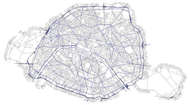
Figure 1: Overlayed drawings of OSM Paris street network (in black) and traffic sensor network (in blue).

We say that the measurement network is a low-resolution network because its links generally correspond to several links in the street network. Conversely, we say that the street network is a high-resolution network. Figure 2 shows that the measurement links are indeed longer than the links of the street network, in general.

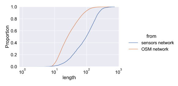
Figure 2: Cumulative distribution of link length (in meters) for both networks in Paris

This leads to the following problem statement.
Input. We consider a high-resolution directed street network $H=(V_{H},E_{H})$ and a low-resolution measurement network $L=(V_{L},E_{L})$ with $|V_{H}|>|V_{L}|$, $|E_{H}|>|E_{L}|$. In addition, each node $v$ in $V_{H}$ or $V_{L}$ has coordinates $p(v)$ in the Euclidean plane, and each link $e$ in $E_{H}$ or $E_{L}$ has a length $l(e)$ in meters.
Output. For each link $e$ in $E_{L}$ we give a subset $m(e)$ of $E_{H}$ of links that we consider to be the streets in $H$ that correspond to the measurement of $e$. We also provide a multi-criteria assessment of each proposed matching.

This problem is very general, and may be very challenging. We however observe in Figure 1 that the two networks are strongly related, and that for each measurement link there is a path in the street network that follows it closely. We therefore make the following assumptions, that we will use to propose a matching algorithm and assess its results.

Our first assumption is that the correct/best matching of a measurement link $(u,v)$ in $L$ is a path in $H$ from a node close to $u$ to a node close to $v$, or conversely. Indeed, each measurement link in $L$ a priori consists of a coarse-grain street that may be divided into a sequence of smaller streets in $H$. Therefore, for a given integer $k$, we will consider in $V_{H}$ the $k$ nearest nodes of each extremity of the measurement link, and match this link with paths in $H$ between these nodes.

Going further, the measurements links correspond to straight pieces of streets and the matching paths should therefore have a length (in meters) similar to the one of the measurement link. This is our second assumption, therefore we will only consider shortest paths, as their length is minimal, like the length of the straight line corresponding to the measurement link.

For the same reason, our third assumption states that the considered shortest paths should be close to straight lines. Therefore, we will avoid taking paths with edges that form important angles, either between them or with the measurement link.

To capture this, we introduce the following notations. Let us consider a candidate path made of nodes $(u_{0},u_{1},u_{2},...,u_{l})$ in $H$ for matching a measurement link $(x,y)$ in $L$. We denote by $\theta_{r}$ the angle between links $(u_{r-1},u_{r})$ and $(u_{r},u_{r+1})$ viewed as segments, and we call it the $r$-th running angle. We denote by $\sigma_{s}$ the angle between the segment corresponding to the measurement link and the one corresponding to the link $(u_{s},u_{s+1})$, and we call it the $s$-th straight-line angle. Notice that running angles and straight-line angles are related by: $\forall i=1..l-2$, $\sigma_{i+1}=\sigma_{i}+\theta_{i+1}$, which implies that $\forall i=1..l-1$, $\sum_{k=1}^{i}\theta_{k}=\sigma_{i}-\sigma_{0}$.

Last but not least, our forth assumption is that the matching path remains close to the considered measurement links all along/throughout the path, therefore we will try to minimize the area between the measurement link and the chosen path.

4 Matching algorithm

We consider two input networks $H=(V_{H},E_{H})$ and $L=(V_{L},E_{L})$, as well as an integer $k$. For any node $x$ in $V_{L}$, we denote by $N_{k}(x)$ the set of the $k$ nearest neighbors (with respect to node coordinates) of $x$ in $V_{H}$. Then, for each link $(u,v)$ in $E_{L}$ we compute the set $P(u,v)$ of all shortest paths in $H$ from any node in $N_{k}(u)$ to any node in $N_{k}(v)$. We also compute $P(v,u)$ the similar set of paths in the other direction. Finally, output the set $m(u,v)$ of links in $E_{H}$ that correspond to the path in $P(u,v)\cup P(v,u)$ that minimizes a given criterion, excluding path with length equal to 0 (ie we took the same node in $N_{k}(u)$ and $N_{k}(v)$).

We consider the following library of criteria, in which each link is viewed as a segment:

length criterion (LC):

the length difference between the considered measurement link and the considered path (where we added to the path length the distance between the path endpoints and the measurement link endpoints)

running angle criterion (RC):

the average running angle with the measurement link over the path;

straight-line criterion (SC):

the average straight-line angle between the links of the path and the measurement link;

area criterion (AC):

the area between the path and the measurement link.

We run the algorithm using one of these criteria but, for each obtained matching of a measurement link, we also output its relevance with respect to all other criteria. In this way, we give precious indications on the quality of proposed matchings, as we illustrate in next section.

5 Results and discussion

We present here the results obtained by running the algorithm above on the Paris street and measurement networks with $k=4$, which is representative of a wide variety of cases. As we compute for each measurement link $2\cdot k^{2}$ shortest paths, we obtain here $32$ candidate paths for matching each of them. Each criterion provides a score for any shortest path, enabling us to analyze and compare them.
We noticed 3 edges from the measurement networks were not successfully matched whichever criterion was used : two are on Rue de Rivoli, and the remaining one is located in Bagnolet interchange. Due to Rue de Rivoli now being unavailable for most vehicules but buses and bikes, it has recently been partly removed from the Paris street graph obtained through OSMnx. Hence, connectivity issues explain the matching failure here as some one-way streets remain around there. As for Bagnolet it clearly is a side effect : increasing the buffering even more would help here as it is in fact impossible to find a path from the points selected during the matching, but it might also possibly create similar issues elsewhere. Overall, it mostly reminds us we need to be aware of structural modifications of street networks over time. These unmatched edges thus explain why we will now consider 5591 (successfully) matched low-res measurement edges out of 5594.

5.1 Score evaluation

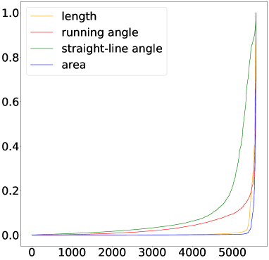
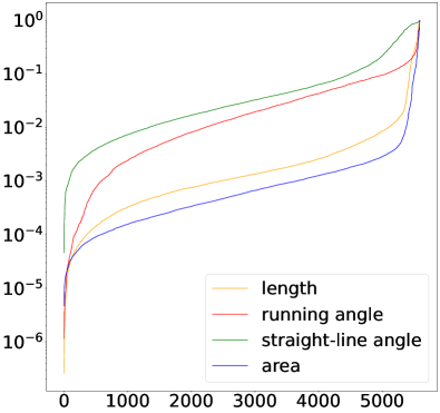
Figure 3: Normalized scores for each criterion with all 5591 matched edges ranked in ascending score order (logarithmic scale of the y-axis is used on the right)

For all cases, we observe in Figure 3 that scores are overall very low (that is logical as we wanted to minimize scores) for most of the paths before a salient increase at the very end. The meaning behind is that the matching algorithm is relevant in picking paths that are overall good candidates for our criteria, and only struggle for a small part of the edges.
It is remarkable that both angle criteria have seemingly quite similar behaviour, while the two others do even more : we might wonder if they provide complementary information, but also if LC and AC are just too strong at discriminating as about 99% of the edges have an almost null score while RC and SC work slightly better at ranking edges.
While no rank correlations were observed for any criterion, the scores are very low similar overall for most of the paths selected by the matching algorithm, making it difficult to unravel any real distinction between them but also to have one standing out. Nonetheless, we can still notice from Figure 3, especially on the right plot, that three different regimes can be observed : the lowest scores on the very left, the highest scores on the very right and then all the others inbetween which are in fact most of the paths.

5.2 Correlation between criteria scores

Figure 4: Correlation scores (normalized to [0,1] for both axis each time) of paths matched using a criterion (on the x-axis) with all other criteria one by one (on the y-axis) : first line is LC, then RC, SC, AC. Red dots correspond to correlation with RC, green with SC, blue with AC, orange with LC. Scores are normalized : both axis are [0,1]. Hence the first red plot on top left corner is the correlation between LC and RC scores for edges matched by minimizing LC. The green one just on its right is the correlation between LC and SC scores from matching minimizing LC, and so forth. To understand how to analyze this figure, from the correlation between LC and RC (top-left corner) we focus on the few reds dots around (1,0). These dots are edges with good RC score, but extremely bad LC score (though LC was the focus of the matching here) : this path has very little angular variation yet it is way too short or long.

On Figure 4, we provide the correlations obtained between the scores of the set of edges matched for a given criterion and the three other scores for that same set. We can notice that LC and AC appear to have a correlated behaviour whatever the criteria used for matching. Applying matching with SC as criterion also seem to efficiently choose edges with fairly good LC and AC scores while on the opposite using AC or LC as criterion for the algorithm picks a set of edges with a wide range of scores - and not necessarily good ones - for RC and SC. We also notice that minimizing RC provides similar yet better results than SC for most criteria, as SC is seemingly more difficult to minimize than others : this is the criterion with the most low-scored edges. On Figure 5, we see the output of the matching minimizing RC, where all the lowest-scoring edges are highlighted for each criteria. Unsurprisingly, lowest-scoring edges are the same for LC and AC. We remark here that all criteria but RC point ring-road edges as part of the worst scores, whereas RC mostly has its worst scores on various places inside the city. It might lead to consider applying AC inside the city and RC on the ring road could be an relevant strategy.

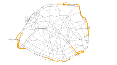
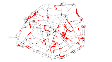
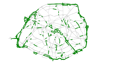
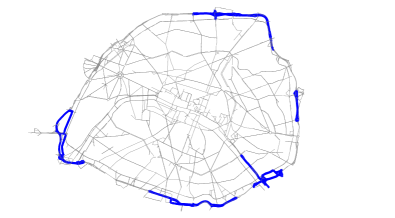
Figure 5: Output of the matching for RC, where the lowest-rated edges for each criteria are highlighted (50 for LC/AC, 300 for RC/SC due to scores on Figure 3).

We can also observe on Figure 6 the location of the lowest-scoring edges for RC but considering all four different matching outputs. First of all, we can simply note that no major mistakes seem to be observed if we compare them to Figure 1. On the one hand, we observe from Figure 6 that LC and AC matching outputs are quite similar yet they both have a tendency to include small links or dead-ends - especially compared to to the two others - as if it was buffered around major roads all around the network, even though AC does it less than LC. On the other hand, RC and SC outputs are also similar and pick more edges than required for the matching but on different places, for example on the outer edge of the ring road where some unrequired loop structures can be seen. Focusing now on the location of lowest-scoring edges for each output, there are a lot of similarities and more specifically we can find some of the largest road infrastructures such as Place de l’Etoile or Porte Maillot, meanwhile the Bercy interchange has an extremely complex topology yet it does not seem to be such an issue. We might need to check closer to understand what is really at stake here.

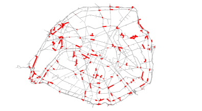
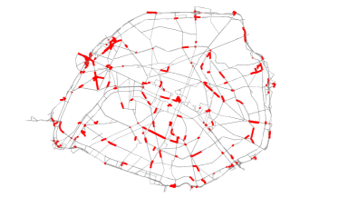
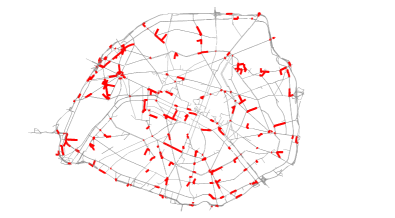
Figure 6: Output of the matching for all criteria, where the 300 lowest-scoring edges for RC are specifically highlighted in red. Top-left is for LC, top-right for RC, bottom-left for SC and bottom-right for AC.

5.3 Visual inspection of limit cases

To provide a deeper understanding of the matching on Figure 6 for each criteria, we study more precisely its behaviour on three cases on Figures 8 7 9 : a significant roundabout at Etoile and two massive interchanges at Bercy and Porte de Maillot. The best output for Etoile clearly is AC as we can observe small mistakes on all the others. This is way more confusing for the two other cases, although we might want to exclude LC as a relevant criterion for such areas considering missing yet expected edges for Bercy, or RC as relevant due to unexpected edges at Etoile and Maillot. However, it is not surprising that the criteria that mostly value straight-lines fail in complex structures such as interchanges. We could even say that the opposite would have been worrying : in fact we are able to detect areas where in any case here, human intervention would be mandatory to ensure no significant mistake is done. It also seem relevant to consider in such infrastructures, our main hypothesis about the difference in resolution between the two networks is no longer valid or at least weaker.

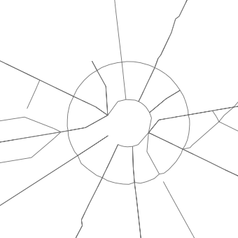
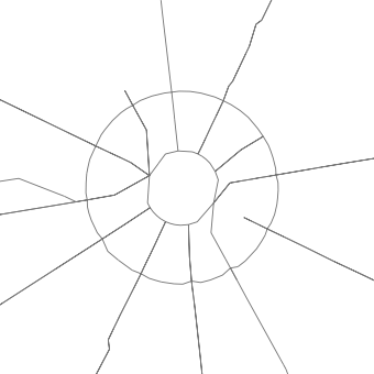
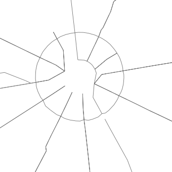
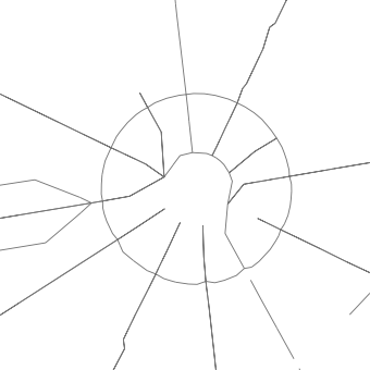
Figure 7: Etoile : OSM and measurements networks - Outputs for LC/RC/SC/AC

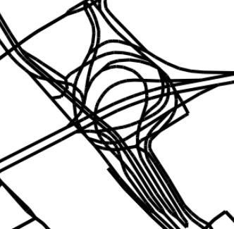
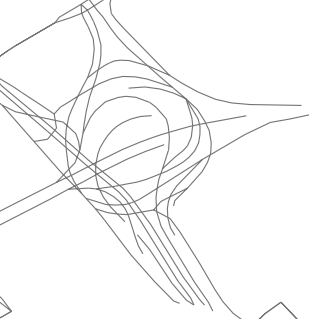
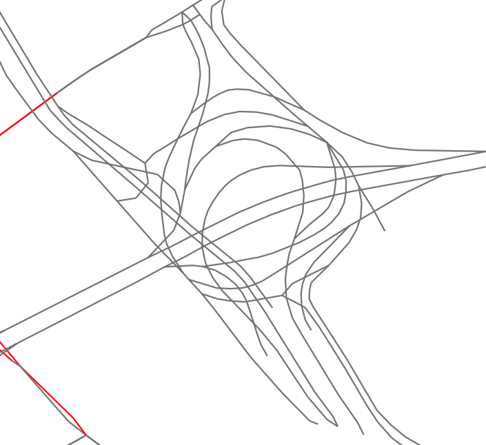
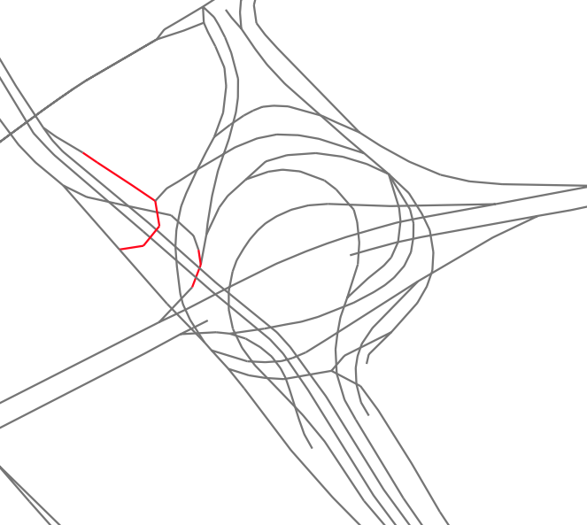
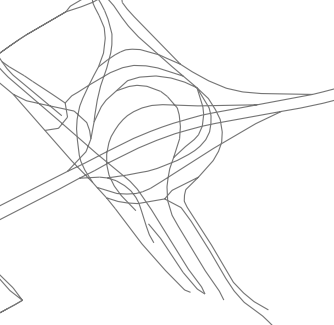
Figure 8: Bercy : OSM and measurements networks - Outputs for LC/RC/SC/AC

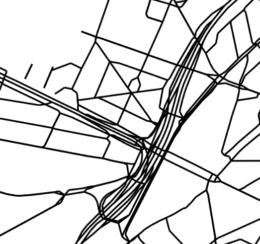
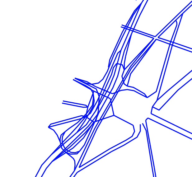
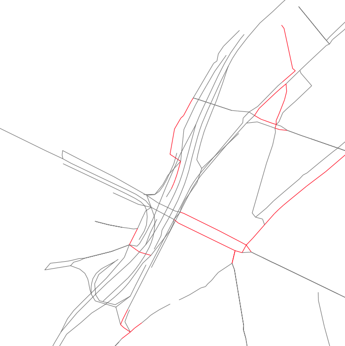
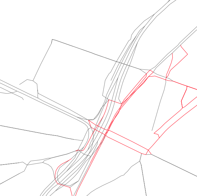
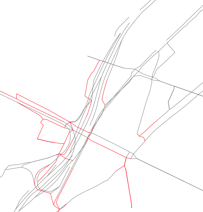
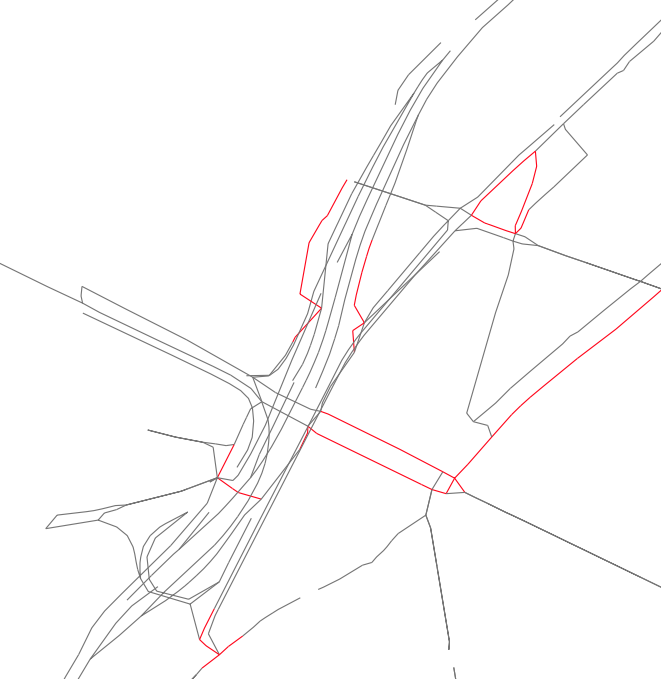
Figure 9: Maillot : OSM and measurements networks - Outputs for LC/RC/SC/AC

6 Related work

Several works explore the limits of OSM [3] [4], including ways to overcome missing data [5]. Based on OSM, OSMnx enables a wide range of studies on urban networks dynamics and properties [6] [7] [8]. Among those, Paris street network and congestions dynamics were previously studied by Taillanter [9] with a network analysis restricted to the measurement network of Paris [10]. Although these results are of interest, it may suffer from sensors geographical distribution heterogeneity and some major traffic road may have been cut, with unknown impact on obtained results. We also note that in spatial network theory and geomatics, Lagesse [11] defined the notion of ”way” to overcome edges in network theory as they induce side-effects due to the arbitrary selection of edges and nodes inside a specific area while ignoring everything around. Ways are designed in order to avoid significant angular variations along a path. The problem we consider in this paper is close to map matching: the problem of matching a curve in an embedded graph. Wenk et al.studied graph modeling of transport data and geometrical algorithms for road networks and it can be encapsulated as map-matching [12] [13], where their goal was to match traffic traces such as GPS trajectories to edges on a graph considering all types of errors that can be found in real datasets. This might include sampling errors, measurement errors, sensors malfunction or more simply lack of precision which all have a strong influence on map-matching [14]. This recent survey on map-matching methods [15] completes what had been done by Houssou in his thesis [16], especially the part about map matching under network topological constraints. What stands out overall is that map-matching is an easy but tedious task for a human operator that needs to be at least partially automated. This is also a classic task in geography and geomatics, where specialists often use GIS (Geographic Information System), such as QGIS , as they allow to tackle our problem by spatially joining two networks [17] although it works a little too much like a black box for beginners and experienced users alike. These methods were further adapted and improved for the specific case of Volunteered Geographic Information such as OSM but only using geometric features [18] or buffering around a link to find matching elements [19]. Nonetheless, we claim matching nodes to edges is not relevant here (although sensors location is provided) as it would necessarily lead to fallacious results, hence edges matching is by far the most appropriate technique for our problem. What makes our work different from classical map-matching, graph matching or GIS methods is that we intend to map low-resolution edges on high-resolution edges : whereas trajectories might be both long and serpentine, measurements are done on smaller - and necessarily way more straight - edges to provide accurate results, and we take advantage of this topological specificity linking both graphs by using shortest paths in our algorithm.

7 Conclusion

We designed a method taking advantage of the specific features of urban networks to accurately solve our problem. We observed in most cases and for most criteria, this task can be automated for a significant part of the graph even if the very end inevitably requires human verification. A significant asset of our method is that anyone can add its own criteria to be tested and compared to the previous ones in order to improve or adapt the algorithm to some specific situation. We also gained insight on all of our assumptions. Nonetheless, it seems quite obvious some external factors might have a strong influence on the results such as map data resolution and precision, the non-planarity of street networks (that may add some confusion to the matching when picking nearest nodes, especially for bridges, tunnels, or interchanges), and the fact that both datasets might differ over time. A major perspective would be to focus on the unambiguity of the matching as it would be valuable to avoid any high-resolution edge to be matched more than once. Otherwise, how can we find which measurement sensor was the most relevant one among several possibilities for any edge ? Indeed, network topology implies that human verification is utterly mandatory to check how the matching is done, making it sometimes difficult to simply design a relevant criteria working perfectly anywhere in the graph. However, most of these problems can be solved by hand and, on the whole, we are able to understand where and why the algorithm works correctly or not. We assume it might be improved either by a relevant combination of criteria with specifically required properties (if not all at the same time) or by hand to avoid significant mistakes. Further work could now explore similar cases in other cities to assess those criteria on various street network topologies and deepen our analysis.

Acknowledgements. This project has received financial support from the CNRS through the MITI interdisciplinary programs and from AID/DGA (Direction Générale de l’Armement). We thank Eric Colin de Verdière and Claire Lagesse for helpful discussions.

References

- [1] OpenStreetMap https://www.openstreetmap.org/
- [2] Boeing, G. (2017). OSMnx: New methods for acquiring, constructing, analyzing, and visualizing complex street networks. Computers, Environment and Urban Systems, 65, 126-139.
- [3] Mooney, P. & Minghini, M. (2017). A review of OpenStreetMap data. Mapping and the citizen sensor, 37-59.
- [4] Antoniou, V. & Skopeliti, A. (2017). The impact of the contribution microenvironment on data quality: the case of OSM. Mapping and the Citizen Sensor, 165-196.
- [5] Funke, S., Schirrmeister, R. & Storandt, S. (2015, July). Automatic extrapolation of missing road network data in OpenStreetMap. In Proceedings of the 2nd International Conference on Mining Urban Data-Volume 1392 (pp. 27-35).
- [6] Vivek, S. & Conner, H. (2022). Urban road network vulnerability and resilience to large-scale attacks. Safety science, 147, 105575
- [7] Alabbad, Y., Mount, J., Campbell, A. M. & Demir, I. (2021). Assessment of transportation system disruption and accessibility to critical amenities during flooding: Iowa case study. Science of the total environment, 793, 148476.
- [8] Neukart, F., Compostella, G., Seidel, C., Von Dollen, D., Yarkoni, S. & Parney, B. (2017). Traffic flow optimization using a quantum annealer. Frontiers in ICT, 4, 29.
- [9] Taillanter, E., & Barthelemy, M. (2021). Empirical evidence for a jamming transition in urban traffic. Journal of the Royal Society Interface, 18(182), 20210391.
- [10] Geographical reference frame for road traffic measurements in Paris : https://opendata.paris.fr/explore/dataset/referentiel-comptages-routiers/information/
- [11] Lagesse, C., Bordin, P. & Douady, S. (2015). A spatial multi-scale object to analyze road networks. Network Science, 3(1), 156-181.
- [12] Ahmed, M., Karagiorgou, S., Pfoser, D., Wenk, C., Ahmed, M., Karagiorgou, S. & Wenk, C. (2015). Map construction algorithms (pp. 1-14). Springer International Publishing.
- [13] Chambers, E., Fasy, B. T., Wang, Y. & Wenk, C. (2020). Map-matching using shortest paths. ACM Transactions on Spatial Algorithms and Systems (TSAS), 6(1), 1-17
- [14] Chen, W., Li, Z., Yu, M. & Chen, Y. (2005). Effects of sensor errors on the performance of map matching. The Journal of Navigation, 58(2), 273-282.
- [15] Chao, P., Xu, Y., Hua, W. & Zhou, X. (2020). A survey on map-matching algorithms. In Databases Theory and Applications: 31st Australasian Database Conference, ADC 2020, Melbourne, VIC, Australia, February 3–7, 2020, Proceedings 31 (pp. 121-133). Springer International Publishing.
- [16] Houssou, N. L. J. (2021). Analyse et modélisation de trajectoires d’utilisateurs dans des systèmes réels (Doctoral dissertation, Université de La Rochelle).
- [17] Jacox, E. H., & Samet, H. (2007). Spatial join techniques. ACM Transactions on Database Systems (TODS), 32(1), 7-es.
- [18] Koukoletsos, T., Haklay, M., & Ellul, C. (2012). Assessing data completeness of VGI through an automated matching procedure for linear data. Transactions in GIS, 16(4), 477-498.
- [19] Abdolmajidi, E., Mansourian, A., Will, J., & Harrie, L. (2015). Matching authority and VGI road networks using an extended node-based matching algorithm. Geo-Spatial Information Science, 18(2-3), 65-80