Well-posedness and stability of abstract thermoelastic delayed systems

Abstract.

In this paper, we consider a stabilization problem of a generalized thermoelastic system (the so called $\alpha$-$\beta$ system) with delay in a part of the coupled system. For each case, we prove the well-posedness of the corresponding system using semigroup approach, then under some sufficient conditions we establish some results of exponential and polynomial stability of the system through a frequency-domain approach. The results are applied to concrete examples in thermoelasticity.

1. Introduction

Let $H$ be a Hilbert space equipped with an inner product $(.,.)_{H}$ and a norm $\|\;\|_{H}$, $A:D(A)\subset H\rightarrow H$ a self-adjoint, strictly positive (unbounded) operator and $(\alpha,\beta)\in[0,1]\times[0,1]$. We consider the following two Cauchy problems modeled, respectively, by the abstract thermoelastic systems with delay given by

$$\left\{\begin{array}[]{ll}u^{\prime\prime}(t)+Au(t-\tau)+aAu^{\prime}(t)-A^{\beta}\theta(t)=0,&\quad t\in(0,+\infty),\\ \theta^{\prime}(t)+A^{\alpha}\theta(t)+A^{\beta}u^{\prime}(t)=0,&\quad t\in(0,+\infty),\\ u(0)=u_{0},u^{\prime}(0)=u_{1},\theta(0)=\theta_{0},&\\ \displaystyle A^{1/2}u(t-\tau)=\phi(t-\tau),&\quad t\in(0,\tau),\end{array}\right.$$ (1.1)

and

$$\left\{\begin{array}[]{ll}u^{\prime\prime}(t)+Au(t)-A^{\beta}\theta(t)=0,&\quad t\in(0,+\infty),\\ \theta^{\prime}(t)+\kappa A^{\alpha}\theta(t-\tau)+aA^{\alpha}\theta(t)+A^{\beta}u^{\prime}(t)=0,&\quad t\in(0,+\infty),\\ u(0)=u_{0},u^{\prime}(0)=u_{1},\theta(0)=\theta_{0},&\\ \displaystyle A^{\alpha/2}\theta(t-\tau)=\psi(t-\tau),&\quad t\in(0,\tau).\end{array}\right.$$ (1.2)

where $\tau>0$ is a constant time delay, $a>0$ and $\kappa>0$. We are interested in the well-posedness of systems (1.1) and (1.2) and the study of the asymptotic behavior of solutions $u,\theta:[0,\infty)\rightarrow H$ as $t\rightarrow\infty$, for $(\beta,\alpha)$ in the region $Q$ where $Q$ is given by

$$Q:=\{(\beta,\alpha)\in[0,1]\times[0,1]\mid 2\beta-\alpha\leq 1\}\quad\text{(Figure \ref{QQ})}.$$

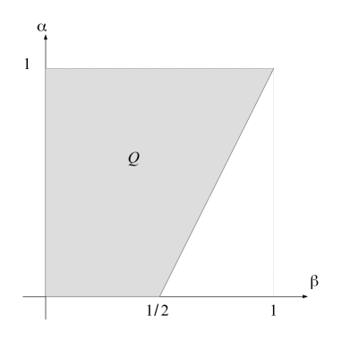
Figure 1. Region $Q$

Note that the regions of the couple $(\beta,\alpha)$ considered for the two delayed $\alpha,\beta$ systems (1.1) and (1.2) cover some concrete examples given in the literature (in the non-delayed form), such as, the thermoelastic plate equations (with $\alpha=\beta=1/2$ and $A=\Delta^{2}$), which is widely discussed since some decades (see e.g. [26, 29, 45, 30, 11, 31]). The choice $H=L^{2}(0,L)$, with $L>0$, $A=-\frac{\partial^{4}}{\partial x^{4}}$, $\alpha=\frac{1}{2}$ and $\beta=0$ corresponds to a one dimensional thermoelastic beam and it was proved that the corresponding system is polynomially stable of order $1$ for various boundary conditions ([23, 35, 34]).

In recent years, several research has been dealing with delayed equations. In fact, delay effects arise in so many applications and physical problems, see e.g. [47, 1] and [2, 8, 9, 10, 40, 18, 13], but may be source of some instabilities ([17, 15, 16, 19, 36, 41, 43]).

In order to ensure well-posedness or stability of a delayed system, many ideas were recently deployed: one can add a non-delay term (see [40] for example). A delayed system can also be stabilized using standard feedback compensating the destabilizing delay effect (see e.g. [9, 2, 36, 37, 38, 39, 32]). Furthermore, recent papers shoes that, under a particular choice of the time delay, we may restitute the exponential stability property (see e.g. [8], [10], [22]).

In [43], Racke considered the $\alpha$-$\beta$ systems with delay

$$\left\{\begin{array}[]{ll}u^{\prime\prime}(t)+Au(t-\tau)-A^{\beta}\theta(t)=0,&\quad t\in(0,+\infty),\\ \theta^{\prime}(t)+A^{\alpha}\theta(t)+A^{\beta}u^{\prime}(t)=0,&\quad t\in(0,+\infty),\end{array}\right.$$ (1.3)

and

$$\left\{\begin{array}[]{ll}u^{\prime\prime}(t)+Au(t)-A^{\beta}\theta(t)=0,&\quad t\in(0,+\infty),\\ \theta^{\prime}(t)+\kappa A^{\alpha}\theta(t-\tau)+A^{\beta}u^{\prime}(t)=0,&\quad t\in(0,+\infty),\end{array}\right.$$ (1.4)

with some initial and boundary conditions. He proved that under the hypothesis that the operator $A$ has a countable complete orthonormal system of eigenfunctions $(e_{j})$ with corresponding eigenvalues $0<\lambda_{j}\rightarrow\infty$ as $j\rightarrow\infty$, systems (1.3) and (1.4) are respectively unstable (not well-posed in the sense of Hadamard) at least in the regions

$$\mathcal{A}_{1}:=\{(\beta,\alpha)\mid 0\leq\beta\leq\alpha\leq 1,\;\alpha\geq\frac{1}{2},\;(\beta,\alpha)\neq(1,1)\}$$

and

$$\mathcal{A}_{2}:=\{(\beta,\alpha)\mid 0\leq\beta\leq\alpha\leq 1,\;(\beta,\alpha)\neq(1,1)\}.$$

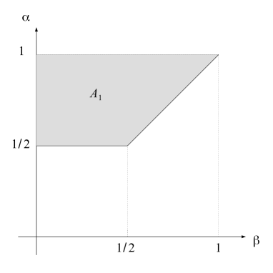
Figure 2. Area of instability $A_{1}$ (with delay and no damping)

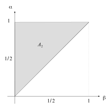
Figure 3. Area of instability $A_{2}$ (with delay and no damping)

However, it is well known that the $\alpha$-$\beta$ system without delay is well posed in the whole region $[0,1]\times[0,1]$. Moreover, in [3] F. A. Khodja et al. identified the region of exponential stability to be

$$S:=\{(\beta,\alpha)\in[0,1]\times[0,1]\mid\max\{1-2\beta,2\beta-1\}\leq\alpha\leq 2\beta\}.$$

Afterwards Hao and Liu [23] (see also [7, 6, 5]) give a classification of the regions of stability and instability (Figure 4). They shewed that the region of polynomial stability is given by

$$R=S_{1}\cup S_{2}:=\{(\beta,\alpha)\in[0,1]\times[0,1]\mid 2\beta<\alpha<1-2\beta\}$$

and the region of instability is given by

$$S_{3}:=\{(\beta,\alpha)\in[0,1]\times[0,1]\mid 0<\alpha<2\beta-1\}.$$

Note that, the region of stability is then, $\framebox{$S\cup S_{1}\cup S_{2}=Q$}.$

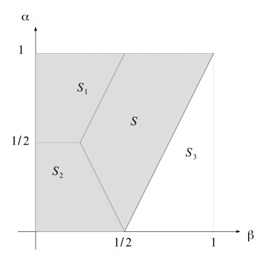
Figure 4. Region of stability and region of instability (no delay & no damping)

Recently K. Ammari et al. give more stability results taking into account the irregularity of the associated operator at the origin [7]. See also [24] for a complete study of the regularity of solutions of the $\alpha$-$\beta$ system, see [46, 35] and some references therein for recent works about stability of abstract thermoelastic systems.

Besides, Racke considered in the same work [43] the one dimensional delayed thermoelastic systems,

$$\left\{\begin{tabular}[]{l}$u_{tt}(x,t)-\alpha u_{xx}(x,t-\tau)+\gamma\theta_{x}(x,t)=0,\;\;\;\;\;\;\text{ in }(0,\ell)\times(0,\infty),$\\ $\theta_{t}(x,t)-\kappa\theta_{xx}(x,t)+\gamma u_{xt}(x,t)=0,\;\;\;\;\;\;\;\;\;\;\;\;\;\text{ in }(0,\ell)\times(0,\infty),$\end{tabular}\right.$$ (1.5)

and

$$\left\{\begin{tabular}[]{l}$u_{tt}(x,t)-\alpha u_{xx}(x,t)+\gamma\theta_{x}(x,t)=0,\;\;\;\;\;\;\text{ in }(0,\ell)\times(0,\infty),$\\ $\theta_{t}(x,t)-\kappa\theta_{xx}(x,t-\tau)+\gamma u_{xt}(x,t)=0,\;\;\;\;\;\;\;\;\;\;\;\;\;\text{ in }(0,\ell)\times(0,\infty).$\end{tabular}\right.$$ (1.6)

He proved also that theses systems are ill-posed (even if $\tau$ is small). However, we know that in the absence of delay, the classical thermoelastic system in one dimension corresponding to (1.5) or (1.6) with $\tau=0$, is well-posed and even exponentially stable (see e.g. [42, 31]).

In order to restitute the well-posedness character and the stability of the one dimensional thermoelastic system (1.5) Khatir and Shel [27] added a Kelvin-Voight damping $-au_{xxt}(x,t)$ to the instable system part and proved that it is not only well-posed (in an appropriate Hilbert space) but also exponentially stable for $a>a_{0}$ (for some positive number $a_{0}$. Rather, Mustapha and Kafini in[33] added to the delayed equation in (1.6) a non delayed term $-a\theta_{xx}(x,t)$ and proved a result of exponential stability under the condition $\kappa<a$.

Even if systems (1.5) and (1.6) are not direct examples of (1.3) and (1.4), we try in this work, to generalize such procedure to (1.3) and (1.4) by adding a Kelvin-Voigt damping term $a\,Au^{\prime}(t)$ to the delayed equation in (1.3) to obtain system (1.1), and a damping term $aA^{\alpha}\theta(t)$ in the second equation in (1.4) to obtain system (1.2). We will prove in particular that, not only the systems (1.1) is well-posed (in an appropriate Hilbert space), but also, the associated semigroup is exponentially stable for $(\beta,\alpha)$ in the region $Q$. In particular the presence of the damping terms $a\,Au^{\prime}(t)$ provides damped systems with better stability than that acquired for $\tau=0$ at least in the regions $S_{1}$ and $S_{2}$. For system (1.2), we will prove that the presence of the damping term $a\,A^{\alpha}\theta(t)$ preserves well-posedness in region $Q$, exponential stability in region $S$, and polynomial stability in region $S_{1}\cup S_{2}$, acquired for $\tau=0$.

Finally, to cover more classical thermoelastic systems, such as, the delayed systems of linear second order-thermoelasticity in one space dimension (1.5) and (1.6), we will consider in this work more general abstract thermoelastic systems with delay of the form

$$\left\{\begin{array}[]{ll}u^{\prime\prime}(t)+Au(t-\tau)+aAu^{\prime}(t)-C\theta(t)=0,&\quad t\in(0,+\infty),\\ \theta^{\prime}(t)+A^{\alpha}\theta(t)+C^{*}u^{\prime}(t)=0,&\quad t\in(0,+\infty),\\ u(0)=u_{0},u^{\prime}(0)=u_{1},\theta(0)=\theta_{0},&\\ \displaystyle B^{*}u(t-\tau)=\phi(t-\tau),&\quad t\in(0,\tau),\end{array}\right.$$ (1.7)

and

$$\left\{\begin{array}[]{ll}u^{\prime\prime}(t)+Au(t)-C\theta(t)=0,&\quad t\in(0,+\infty),\\ \theta^{\prime}(t)+\kappa A^{\alpha}\theta(t-\tau)+aA^{\alpha}\theta(t)+C^{*}u^{\prime}(t)=0,&\quad t\in(0,+\infty),\\ u(0)=u_{0},u^{\prime}(0)=u_{1},\theta(0)=\theta_{0},&\\ \displaystyle B^{*}\theta(t-\tau)=g_{0}(t-\tau),&\quad t\in(0,\tau),\end{array}\right.$$ (1.8)

where $B:D(B)\subset H\rightarrow H$, $C:D(C)\subset H\rightarrow H$ are closed densely defined operators on $H$ satisfying some properties for each system, $B^{*}$ is the adjoint of $B$, and with $A=BB^{*}$ in (1.7) and $A^{\alpha}=BB^{*}$ in (1.8). The corresponding non delayed system (where $\tau=0$) was studied before in a more general form (by taking an operator $A_{1}$ instead of $A^{\alpha}$), see e.g. [21, 44, 28]) and [4] and some references therein. We will give sufficient conditions on $A^{\alpha}$, $B$ and $C$ which ensure the exponential (or polynomial) stability of the associated semigroup, and which can be compared to those proposed in [4] for $\tau=0$.

The paper is organized as follows. The second and third sections deals with the well-posedness and stability of the problems (1.1) and (1.2) respectively. We end each section by a general abstract system and applications.

In the sequel, $\framebox{$(\beta,\alpha)\in Q:=\{(\beta,\alpha)\in[0,1]\times[0,1]\mid 2\beta-\alpha\leq 1\}$}$.

2. Well-posedness and stability of the problem (1.1)

2.1. Well-posedness of the coupled system (1.1)

We introduce, as in [8], the auxiliary variable

$$z(\rho,t)=A^{1/2}u(t-\tau\rho),\quad\rho\in(0,1),t>0.$$

Then, problem (1.2) is equivalent to

$$u^{\prime\prime}(t)+A^{1/2}z(1,t)+aAu^{\prime}(t)-A^{\beta}\theta(t)=0,\quad t>0,$$

$$\theta^{\prime}(t)+A^{\alpha}\theta(t)+A^{\beta}u^{\prime}(t)=0,\quad t>0,$$

$$\tau z_{t}(\rho,t)+z_{\rho}(\rho,t)=0,\quad(\rho,t)\in(0,1)\times(0,+\infty),$$

$$u(0)=u_{0},u^{\prime}(0)=u_{1},\theta(0)=\theta_{0},$$

$$z(\rho,0)=\phi(-\tau\rho),\quad\rho\in(0,1),$$

$$z(0,t)=A^{1/2}u(t),\quad t>0.$$

Define

$$U=(u,u^{\prime},\theta,z)^{\top},$$

Then, problem (1.1) can be formulated as a first order system of the form

$$\left\{\begin{array}[]{ll}U^{\prime}(t)=\mathcal{A}_{\alpha,\beta}U(t),\,t>0,&\\ \displaystyle U(0)=\big{(}u_{0},u_{1},\theta_{0},\phi(-\tau\cdot)\big{)}^{\top},\end{array}\right.$$ (2.1)

where the operator $\mathcal{A}_{\alpha,\beta}$ is defined by

$$\mathcal{A}_{\alpha,\beta}\left(\begin{array}[]{c}u\\ v\\ \theta\\ z\\ \end{array}\right)=\left(\begin{array}[]{c}v\\ \displaystyle-A^{1/2}\big{(}z(1)+aA^{1/2}v-A^{\beta-\frac{1}{2}}\theta\big{)}\\ -A^{\alpha/2}\left(A^{\alpha/2}\theta+A^{\beta-\frac{\alpha}{2}}v\right)\\ \displaystyle-\frac{1}{\tau}z_{\rho}\\ \end{array}\right),$$

with domain

$$D(\mathcal{A}_{\alpha,\beta})=\left\{\begin{array}[]{c}(u,v,\theta,z)^{\top}\in D(A^{1/2})\times D(A^{1/2})\times D(A^{\alpha/2})\times H^{1}\big{(}(0,1),H\big{)}:\quad z(0)=A^{1/2}u,\\ \displaystyle z(1)+aA^{1/2}v-A^{\beta-\frac{1}{2}}\theta\in D(A^{\frac{1}{2}}),\quad\textrm{ and }\quad A^{\alpha/2}\theta+A^{\beta-\frac{\alpha}{2}}v\in D(A^{\alpha/2})\end{array}\right\},$$

in the Hilbert space

$$\mathcal{H}=D(A^{1/2})\times H\times H\times L^{2}\big{(}(0,1),H\big{)},$$

equipped with the scalar product

$$\big{(}(u,v,\theta,z)^{\top},(u_{1},v_{1},\theta_{1},z_{1})^{\top}\big{)}_{\mathcal{H}}=\big{(}A^{1/2}u,A^{1/2}u_{1}\big{)}_{H}+(v,v_{1})_{H}+(\theta,\theta_{1})_{H}+\xi\int_{0}^{1}(z,z_{1})_{H}d\rho,$$

where $\xi>0$ is a parameter that will be fixed later on.

Remark 2.1.

If $(\beta,\alpha)\in[0,1/2]\times[0,1]$ and $\beta\leq\alpha$, then $A^{\beta-\frac{\alpha}{2}}v\in D(A^{\alpha/2})$, hence $\mathcal{A}_{\alpha,\beta}$ is reduced to

$$\mathcal{A}_{\alpha,\beta}\left(\begin{array}[]{c}u\\ v\\ \theta\\ z\\ \end{array}\right)=\left(\begin{array}[]{c}v\\ \displaystyle-A^{1/2}\big{(}z(1)+aA^{1/2}v\big{)}+A^{\beta}\theta\\ -A^{\alpha}\theta-A^{\beta}v\\ \displaystyle-\frac{1}{\tau}z_{\rho}\\ \end{array}\right),$$

with domain

$$D(\mathcal{A}_{\alpha,\beta})=\left\{\begin{array}[]{c}(u,v,\theta,z)^{\top}\in D(A^{1/2})\times D(A^{1/2})\times D(A^{\alpha})\times H^{1}\big{(}(0,1),H\big{)}:\\ \displaystyle z(0)=A^{1/2}u,\quad\textrm{ and }\quad z(1)+aA^{1/2}v\in D(A^{\frac{1}{2}})\end{array}\right\}.$$

Lemma 2.1.

If $\displaystyle\xi\geq\frac{2\tau}{a}$, then $\mathcal{A}_{\beta,\alpha}-mId$ is dissipative in $\mathcal{H}$, where $m=\frac{1}{a}+\frac{\xi}{2\tau}$.

Proof.

Take $U=(u,v,\theta,z)^{\top}\in D(\mathcal{A}_{\alpha,\beta})$. We have

$$\displaystyle\big{(}\mathcal{A}_{\alpha,\beta}U,U\big{)}_{\mathcal{H}} = \big{(}A^{1/2}v,A^{1/2}u\big{)}_{H}-\big{(}z(1)+aA^{1/2}v,A^{1/2}v\big{)}_{H}+(A^{\beta-\frac{1}{2}}\theta,A^{\frac{1}{2}}v)_{H}-(A^{\alpha/2}\theta,A^{\alpha/2}\theta)_{H}$$

$$- (A^{\frac{1}{2}}v,A^{\beta-\frac{1}{2}}\theta)_{H}-\frac{\xi}{\tau}\int_{0}^{1}(z_{\rho},z)_{H}d\rho.$$

Using the Young’s inequality and that $\displaystyle z(0)=A^{1/2}u$, we find that, for every $\varepsilon>0$,

$$\displaystyle Re\big{(}\mathcal{A}_{\alpha,\beta}U,U\big{)}_{\mathcal{H}} = \big{(}A^{1/2}v,A^{1/2}u\big{)}_{H}-\big{(}z(1),A^{1/2}v\big{)}_{H}-a\|A^{1/2}v\|^{2}_{H}-\|A^{\frac{\alpha}{2}}\theta\|^{2}_{H}$$

$$- \frac{\xi}{2\tau}\|z(1)\|^{2}_{H}+\frac{\xi}{2\tau}\|A^{1/2}u\|^{2}_{H}$$

$$\leq (\varepsilon-a)\|A^{1/2}v\|_{H}^{2}+\left(\frac{1}{2\varepsilon}+\frac{\xi}{2\tau}\right)\|A^{1/2}u\|_{H}^{2}-\|A^{\frac{\alpha}{2}}\theta\|_{H}^{2}+\left(\frac{1}{2\varepsilon}-\frac{\xi}{2\tau}\right)\|z(1)\|^{2}_{H}.$$

Choosing $\displaystyle\varepsilon=\frac{a}{2}$, we get

$$Re\big{(}\mathcal{A}_{\alpha,\beta}U,U\big{)}_{\mathcal{H}}\leq-\frac{a}{2}\|A^{1/2}v\|_{H}^{2}+\left(\frac{1}{a}+\frac{\xi}{2\tau}\right)\|A^{1/2}u\|_{H}^{2}-\|A^{\frac{\alpha}{2}}\theta\|_{H}^{2}+\left(\frac{1}{a}-\frac{\xi}{2\tau}\right)\|z(1)\|^{2}_{H}.$$

Then, we choose $\xi$ such that $\displaystyle\frac{1}{a}-\frac{\xi}{2\tau}\leq 0$, that is $\displaystyle\xi\geq\frac{2\tau}{a}$. Furthermore, we take $\displaystyle m=\frac{1}{a}+\frac{\xi}{2\tau}$ which leads to

$$Re\big{(}\mathcal{A}_{\alpha,\beta}U,U\big{)}_{\mathcal{H}}\leq-\frac{a}{2}\|A^{1/2}v\|_{H}^{2}+\left(\frac{1}{a}-\frac{\xi}{2\tau}\right)\|z(1)\|^{2}_{H}-\|A^{\frac{\alpha}{2}}\theta\|_{H}^{2}+m\|A^{1/2}u\|_{H}^{2}.$$ (2.2)

This readily shows the dissipativeness of the operator $\mathcal{A}_{\alpha,\beta}-mId$. ∎

Lemma 2.2.

Assume that $a\geq\tau$. Then

$$\mathbb{C}_{0}\subset\rho(\mathcal{A}_{\alpha,\beta})$$

Proof.

Since $\mathcal{A}_{\alpha,\beta}-mId$ is dissipative, it suffices to prove that $\lambda Id-\mathcal{A}_{\alpha,\beta}$ is bijective for every $\lambda\in\mathbb{C}_{0}$.

To this end, we fix $(f,g,p,h)^{\top}\in\mathcal{H}$ and we seek a unique solution $U=(u,v,\theta,z)^{\top}\in D(\mathcal{A}_{\alpha,\beta})$ of

$$\big{(}\lambda Id-\mathcal{A}_{\alpha,\beta}\big{)}\left(\begin{array}[]{c}u\\ v\\ \theta\\ z\\ \end{array}\right)=\left(\begin{array}[]{c}f\\ g\\ p\\ h\\ \end{array}\right),$$

that is verifying

$$\left\{\begin{array}[]{ll}\lambda u-v=f,&\\ \displaystyle\lambda v+A^{1/2}\big{(}z(1)+aA^{1/2}v-A^{\beta-\frac{1}{2}}\theta\big{)}=g,&\\ \lambda\theta+A^{\alpha/2}\left(A^{\alpha/2}\theta+A^{\beta-\frac{\alpha}{2}}v\right)=p,&\\ \displaystyle\lambda z+\frac{1}{\tau}z_{\rho}=h.&\end{array}\right.$$ (2.3)

Suppose that we have found $u$ with the appropriate regularity. Then,

$$v=\lambda u-f.$$ (2.4)

To determine $z$, we set $\displaystyle z(0)=A^{1/2}u$. Then, by $(\ref{s9})_{4}$, we obtain

$$z(\rho)=e^{-\lambda\tau\rho}A^{1/2}u+\tau e^{-\lambda\tau\rho}\int_{0}^{\rho}h(s)e^{\lambda\tau s}ds.$$ (2.5)

In particular, we have

$$z(1)=e^{-\lambda\tau}A^{1/2}u+z_{0}$$ (2.6)

with

$$z_{0}=\tau e^{-\lambda\tau}\int_{0}^{1}h(s)e^{\lambda\tau s}ds\in L^{2}\big{(}(0,1),H\big{)}.$$ (2.7)

Using (2.4) in (2.3)₂, we see that $u$ satisfies

$$\lambda^{2}(u,x)_{H}-\lambda(f,x)_{H}+(z(1)+\lambda aA^{1/2}u-A^{\beta-1/2}\theta,A^{1/2}x)_{H}-a(A^{1/2}f,A^{1/2}x)_{H}=(g,x)_{H},$$ (2.8)

for all $\displaystyle x\in D(A^{1/2})$.

Substituting (2.6) in (2.8), we get

$$\lambda^{2}(u,x)_{H}+(e^{-\lambda\tau}+\lambda a)(A^{1/2}u,A^{1/2}x)_{H}-(A^{\beta-1/2}\theta,A^{1/2}x)_{H}=(\lambda f+g,x)+(aA^{1/2}f-z_{0},A^{1/2}x)_{H}$$ (2.9)

for all $\displaystyle x\in D(A^{1/2})$.

Moreover, plugging (2.4) in (2.3)₃, we obtain

$$\lambda(\theta,y)_{H}+(A^{\alpha/2}\theta,A^{\alpha/2}y)_{H}+\lambda(A^{\beta-\frac{\alpha}{2}}u,A^{\alpha/2}y)_{H}=(p,y)_{H}+(A^{\beta-\frac{\alpha}{2}}f,A^{\alpha/2}y)_{H}$$ (2.10)

for all $\displaystyle y\in D(A^{\alpha/2})$.

Next, summing (2.10) and (2.9) multiplied by $\displaystyle\overline{\lambda}$, to get

$$b\big{(}(u,\theta),(x,y)\big{)}=F(x,y)$$ (2.11)

with

$$b\big{(}(u,\theta),(x,y)\big{)} = \lambda|\lambda|^{2}(u,x)_{H}+(\overline{\lambda}e^{-\lambda\tau}+|\lambda|^{2}a)(A^{1/2}u,A^{1/2}x)_{H}-\overline{\lambda}(A^{\beta-1/2}\theta,A^{1/2}x)_{H}$$

$$+ \lambda(\theta,y)_{H}+(A^{\frac{\alpha}{2}}\theta,A^{\frac{\alpha}{2}}y)_{H}+\lambda(A^{1/2}u,A^{\beta-1/2}y)_{H},$$

and

$$F(x,y)=\overline{\lambda}(\lambda f+g,x)_{H}+\overline{\lambda}(aA^{1/2}f-z_{0},A^{1/2}x)_{H}+(p,y)_{H}+(A^{\beta-\frac{\alpha}{2}}f,A^{\alpha/2}y)_{H}.$$

The space

$$\mathcal{F}=D(A^{1/2})\times D(A^{\frac{\alpha}{2}})$$

endowed with the inner product

$$\big{(}(x,y),(x_{1},y_{1})\big{)}_{\mathcal{F}}=(A^{1/2}x,A^{1/2}x_{1})_{H}+(x,x_{1})_{H}+(A^{\frac{\alpha}{2}}y,A^{\frac{\alpha}{2}}y_{1})_{H}+(y,y_{1})_{H}$$

is a Hilbert space.

Using that $2\beta\leq\alpha+1$, we claim that the sesquilinear form $b$ is continuous on $\mathcal{F}\times\mathcal{F}$. In fact, we have

$$\big{|}b\big{(}(u,\theta),(x,y)\big{)}\big{|}\leq M\|(u,\theta)\|_{\mathcal{F}}\|(x,y)\|_{\mathcal{F}},\quad\forall(u,\theta),(x,y)\in\mathcal{F}\times\mathcal{F},$$

for some positive constant $M$. The anti-linear form $F$ is also clearly continuous on the Hilbert space $\mathcal{F}$.

Now, it is clear that for all $(x,y)\in\mathcal{F}$, we have

$$Re\big{(}b\big{(}(x,y),(x,y)\big{)}\big{)}=\textrm{Re}(\lambda)|\lambda|^{2}\|x\|_{H}^{2}+\big{(}\textrm{Re}(\overline{\lambda}e^{-\lambda\tau})+|\lambda|^{2}a\big{)}\|A^{1/2}x\|_{H}^{2}+\textrm{Re}(\lambda)\|y\|_{H}^{2}+\|A^{\frac{\alpha}{2}}y\|_{H}^{2}.$$ (2.12)

To prove that $b$ is coercive, it suffices to prove that $\textrm{Re}(\overline{\lambda}e^{-\lambda\tau})+|\lambda|^{2}a>0$.

First, we have

$$\textrm{Re}(\overline{\lambda}e^{-\lambda\tau})+|\lambda|^{2}a\geq|\lambda|\left(|\lambda|a-1\right)>0$$

for $|\lambda|>\frac{1}{a}$.

Now, we suppose that $|\lambda|\leq\frac{1}{a}$ and putting $\lambda=r+is,\quad(r,s)\in\mathbb{R}_{+}^{\ast}\times\mathbb{R}$. Since we assume that $a\geq\tau$, we have $|s\tau|\leq 1$ and moreover

$$\textrm{Re}(\overline{\lambda}e^{-\lambda\tau})+|\lambda|^{2}a = (r^{2}+s^{2})a+\big{(}r\cos(s\tau)-s\sin(s\tau)\big{)}e^{-r\tau}$$

$$\geq e^{-r\tau}r\cos(s\tau)+\left(a-\tau\right)s^{2}+r^{2}a$$

$$> \left(a-\tau\right)s^{2}\geq 0.$$

We conclude that, for all $\lambda\in\mathbb{C}$ such that $\textrm{Re}(\lambda)>0$, we have

$$\textrm{Re}(\overline{\lambda}e^{-\lambda\tau})+|\lambda|^{2}a>0$$ (2.13)

for $a\geq\tau$.

By using (2.13) in (2.12), we deduce that $b$ is coercive on $\mathcal{F}\times\mathcal{F}$. By the Lax-Milgram lemma, equation (2.11) has a unique solution $(u,\theta)\in\mathcal{F}$.

We define $v$ by (2.4) that belongs to $D(A^{1/2})$ and $z$ by (2.5) that belongs to $H^{1}(0,1;H)$

Now, if we take $x=0$ in (2.11), we get

$$(A^{\frac{\alpha}{2}}\theta-A^{\beta-\frac{\alpha}{2}}v,A^{\frac{\alpha}{2}}y)_{H}=(p-\lambda\theta,y)_{H},\quad\forall y\in D(A^{\frac{\alpha}{2}}).$$

It follows that

$$A^{\frac{\alpha}{2}}\theta-A^{\beta-\frac{\alpha}{2}}v\in D(A^{\alpha/2})\quad\textrm{ and }\quad A^{\alpha/2}\left(A^{\frac{\alpha}{2}}\theta-A^{\beta-\frac{\alpha}{2}}v\right)+\lambda\theta=p.$$

Next, taking $y=0$ in (2.11) divided by $\overline{\lambda}$ leads to

$$(aA^{1/2}v+z(1)-A^{\beta-\frac{1}{2}}\theta,A^{1/2}x)_{H}=(g-\lambda v,x)_{H},\quad\forall x\in D(A^{1/2}).$$

Thus, we get

$$aA^{1/2}v+z(1)-A^{\beta-\frac{1}{2}}\theta\in D(A^{1/2})\quad\textrm{ and }\quad A^{1/2}\big{(}aA^{1/2}v+z(1)-A^{\beta-\frac{1}{2}}\theta\big{)}+\lambda v=g.$$

We conclude that $\lambda Id-\mathcal{A}_{\alpha,\beta}$ is bijective for all $\lambda\in\mathbb{C}$ such that $\textrm{Re}(\lambda)>0$ (in particular, $\mathcal{A}_{\alpha,\beta}-mI$ is m-dissipative).

∎

Since the operator $\mathcal{A}_{\alpha,\beta}-mI$ is m-dissipative, it generates a $\mathcal{C}_{0}$-semigroup of contractions on $\mathcal{H}$. Then we have the following result:

Proposition 2.1.

For $(\beta,\alpha)\in Q$, $a\geq\tau$ and $\displaystyle\xi\geq\frac{2\tau}{a}$, the system (1.1) is well-posed. More precisely, the operator $\mathcal{A}_{\alpha,\beta}$ generates a $\mathcal{C}_{0}$-semigroup on $\mathcal{H}$. Hence, for every $(u_{0},v_{0},\theta_{0},z_{0})\in\mathcal{H}$, there exists a unique solution $(u,v,\theta,z)\in\mathcal{C}\big{(}(0,+\infty),\mathcal{H}\big{)}$ of (2.1). Moreover, if $(u_{0},v_{0},\theta_{0},z_{0})\in D(\mathcal{A}_{\alpha,\beta})$, then we have $(u,v,\theta,z)\in\mathcal{C}\big{(}(0,+\infty),D(\mathcal{A}_{\alpha,\beta})\big{)}\cap\mathcal{C}^{1}\big{(}(0,+\infty),\mathcal{H}\big{)}$.

2.2. Exponential stability of the delayed coupled system (1.1)

First, we recall the following frequency domain result for uniform stability from [25], Theorem. 8.1.4, of a $\mathcal{C}_{0}$-semigroup $e^{t\mathcal{L}}$ on a Hilbert space:

Lemma 2.3.

A $\mathcal{C}_{0}$ semigroup $e^{t\mathcal{L}}$ on a Hilbert space $G$ satisfies

$$\|e^{t\mathcal{L}}\|_{\mathcal{L}(G)}\leq Ce^{-wt}$$

for some constants $C>0$ and $w>0$ if and only if

$$\mathbb{C}_{0}:=\big{\{}\lambda\in\mathbb{C}\mid\textrm{Re}(\lambda)>0\big{\}}\subset\rho(\mathcal{L})$$ (2.14)

and

$$\underset{\textrm{Re}(\lambda)>0}{\sup}\|(\lambda I-\mathcal{L})^{-1}\|_{\mathcal{L}(G)}<\infty,$$ (2.15)

where $\rho(\mathcal{L})$ denotes the resolvent set of the operator $\mathcal{L}$.

Now, we can state our main result.

Theorem 2.1.

For $(\beta,\alpha)\in Q$, $a\geq\tau$ and $\displaystyle\xi\geq\frac{2\tau}{a}$, the system (2.1) is exponentially stable.

Proof.

The condition (2.14) is satisfied (Lemma 2.2).

Now, we suppose that condition (2.15) is false. Then, there exists a sequence of complex numbers $\lambda_{n}$ such that $\textrm{Re}(\lambda_{n})\geq 0$, $|\lambda_{n}|\rightarrow+\infty$ and a sequence of vectors $U_{n}=(u_{n},v_{n},\theta_{n},z_{n})^{t}\in D(\mathcal{A}_{\alpha,\beta})$ with

$$\|A^{1/2}u_{n}\|^{2}_{H}+\|v_{n}\|^{2}_{H}+\|\theta_{n}\|_{H}^{2}+\xi\int_{0}^{1}\|z_{n}(\rho)\|_{H}^{2}=1,\quad\forall n\geq 1,$$ (2.16)

and such that

$$\underset{n\rightarrow+\infty}{\lim}\big{\|}(\lambda_{n}I-\mathcal{A}_{\alpha,\beta})U_{n}\big{\|}_{H}=0,$$ (2.17)

i.e.,

$$\lambda_{n}A^{1/2}u_{n}-A^{1/2}v_{n}\equiv f_{n}\rightarrow 0\textrm{ in }H,$$ (2.18)

$$\lambda_{n}v_{n}+A^{1/2}\big{(}z_{n}(1)+aA^{1/2}v_{n}-A^{\beta-\frac{1}{2}}\theta_{n}\big{)}\rightarrow 0\textrm{ in }H,$$ (2.19)

$$\lambda_{n}\theta_{n}+A^{\alpha/2}\big{(}A^{\alpha/2}\theta_{n}+A^{\beta-\frac{\alpha}{2}}v_{n}\big{)}\rightarrow 0\textrm{ in }H,$$ (2.20)

$$\lambda_{n}z_{n}+\frac{1}{\tau}\partial_{\rho}z_{n}\equiv h_{n}\rightarrow 0\textrm{ in }L^{2}\big{(}(0,1)H\big{)}.$$ (2.21)

Since $\bigg{|}\big{(}(\lambda_{n}I-\mathcal{A}_{\alpha,\beta})U_{n},U_{n}\big{)}_{\mathcal{H}}\bigg{|}\geq\textrm{Re}(\lambda_{n})-\textrm{Re}(\mathcal{A}_{\alpha,\beta}U_{n},U_{n})_{\mathcal{H}}$, then, using (2.2) and (2.18), we obtain that

$$\displaystyle\bigg{|}\big{(}(\lambda_{n}I-\mathcal{A}_{\alpha,\beta})U_{n},U_{n}\big{)}_{\mathcal{H}}\bigg{|} \geq \textrm{Re}(\lambda_{n})+\frac{a}{2}\|A^{1/2}v_{n}\|_{H}^{2}+\left(\frac{\xi}{2\tau}-\frac{1}{a}\right)\|z_{n}(1)\|_{H}^{2}+\|A^{\frac{\alpha}{2}}\theta_{n}\|_{H}^{2}-m\|A^{1/2}u_{n}\|_{H}^{2}$$

$$\geq \textrm{Re}(\lambda_{n})+\left(\frac{a}{2}-\frac{2m}{|\lambda_{n}|}\right)\|A^{1/2}v_{n}\|_{H}^{2}-\frac{2m}{|\lambda_{n}|}\|f_{n}\|_{H}^{2}+\left(\frac{\xi}{2\tau}-\frac{1}{a}\right)\|z_{n}(1)\|_{H}^{2}$$

$$+\|A^{\frac{\alpha}{2}}\theta_{n}\|_{H}^{2}.$$

Note that there exists $n_{0}\in\mathbb{N}$ such that $\displaystyle\frac{a}{2}-\frac{2m}{|\lambda_{n}|}\geq\frac{a}{4}$ for all $n\geq n_{0}$. Thus, for $n\geq n_{0}$, we get

$$\bigg{|}\big{(}(\lambda_{n}I-\mathcal{A}_{\alpha,\beta})U_{n},U_{n}\big{)}_{\mathcal{H}}\bigg{|} \geq \textrm{Re}(\lambda_{n})+\frac{a}{4}\|A^{1/2}v_{n}\|_{H}^{2}-\frac{2m}{|\lambda_{n}|}\|f_{n}\|_{H}^{2}$$ (2.22)

$$+ \left(\frac{\xi}{2\tau}-\frac{1}{a}\right)\|z_{n}(1)\|_{H}^{2}+\|A^{\frac{\alpha}{2}}\theta_{n}\|_{H}^{2},$$

which further leads to

$$A^{1/2}v_{n}\underset{n\rightarrow+\infty}{\rightarrow}0\;\;\quad\textrm{ and }\quad A^{\frac{\alpha}{2}}\theta_{n}\underset{n\rightarrow+\infty}{\rightarrow}0\textrm{ in }H,$$ (2.23)

(we have used the estimate (2.17) in (2.22)). Then, it follows

$$v_{n}\underset{n\rightarrow+\infty}{\rightarrow}0\quad\textrm{ and }\quad\theta_{n}\underset{n\rightarrow+\infty}{\rightarrow}0\textrm{ in }H.$$ (2.24)

Furthermore,

$$A^{1/2}u_{n}\underset{n\rightarrow+\infty}{\rightarrow}0\textrm{ in }H,$$ (2.25)

due to (2.18).

By integration of the identity (2.21), we obtain

$$z_{n}(\rho)=A^{1/2}u_{n}e^{-\lambda_{n}\rho}+\tau\int_{0}^{\rho}e^{-\tau\lambda_{n}(\rho-s)}h_{n}(s)ds.$$ (2.26)

Combining (2.25) and (2.26), we get

$$\|z_{n}\|_{L^{2}\big{(}(0,1),H\big{)}}^{2}\leq 2\|A^{1/2}u_{n}\|_{H}^{2}+2\tau^{2}\|h_{n}\|_{L^{2}\big{(}(0,1),H\big{)}}^{2}\displaystyle\underset{n\rightarrow+\infty}{\rightarrow}0.$$ (2.27)

Finally, we have shown that $\|U_{n}\|_{\mathcal{H}}\underset{n\rightarrow+\infty}{\rightarrow}0$ which clearly contradicts (2.16). Thus, (2.15) holds and the proof of Theorem 2.1 is then finished. ∎

Remark 2.2.

Adding the Kelvin-Voigt damping $aAu^{\prime}(t)$ to $Au(t-\tau)$ not only restores the exponential stability in the region $S$, but improves the stability in the $S_{1}\cup S_{2}$ which become exponential.

2.3. Some related systems

We consider the following system

$$\left\{\begin{array}[]{ll}u^{\prime\prime}(t)+Au(t-\tau)+aAu^{\prime}(t)-C\theta(t)=0,&\quad t\in(0,+\infty),\\ \theta^{\prime}(t)+A^{\alpha}\theta(t)+C^{*}u^{\prime}(t)=0,&\quad t\in(0,+\infty),\\ u(0)=u_{0},u^{\prime}(0)=u_{1},\theta(0)=\theta_{0},&\\ \displaystyle B^{*}u(t-\tau)=\phi(t-\tau),&\quad t\in(0,\tau),\end{array}\right.$$ (2.28)

where $\tau>0$ is a constant time delay and $a>0$, $B:D(B)\subset H\rightarrow H$ and $C:D(C)\subset H\rightarrow H$ are closed densely defined linear operators with $B^{*}$ and $C^{*}$ are the adjoints of $B$ and $C$. We suppose that $A=BB^{*}$. Formally, system (2.28) can be seen as a generalization of the delayed $\alpha$-$\beta$ system (1.1).

We suppose also that

$$\exists\,c_{1}>0\;\hbox{ s.t. }\;\|B^{*}v\|_{H}\geq c_{1}\|v\|_{H},\;\;\forall\ v\in D(B^{*}),$$ (2.29)

$$D(A^{\alpha})\subset D(C),\quad D(B^{*})\subset D(C^{*})$$

and

$$\exists\,c_{2}>0\;\hbox{ s.t. }\;\|C^{*}v\|_{H}\leq c_{2}\|B^{*}v\|_{H},\;\;\forall\ v\in D(B^{*}).$$ (2.30)

2.3.1. Well-posedness

Here we take

$$z(\rho,t):=B^{*}u(t-\tau\rho),\quad\rho\in(0,1),t>0.$$

Then, problem (2.28) is equivalent to

$$\left\{\begin{array}[]{ll}u^{\prime\prime}(t)+Bz(1,t)+aBB^{*}u^{\prime}(t)-C\theta(t)=0,&t>0,\\ \theta^{\prime}(t)+A^{\alpha}\theta(t)+C^{*}u^{\prime}(t)=0,&t>0,\\ \tau z_{t}(t,\rho)+z_{\rho}(\rho,t)=0,&(\rho,t)\in(0,1)\times(0,+\infty),\\ u(0)=u_{0},u^{\prime}(0)=u_{1},\theta(0)=\theta_{0},&\\ z(\rho,0)=\phi(-\tau\rho),&\rho\in(0,1),\\ z(0,t)=B^{*}u(t),&\quad t>0.\end{array}\right.$$ (2.31)

Define $U=(u,u^{\prime},\theta,z)^{\top}$, then problem (2.31) can be formulated as a first order system of the form

$$\left\{\begin{array}[]{ll}U^{\prime}=\mathcal{A}U,&\\ \displaystyle U(0)=\big{(}u_{0},u_{1},\theta_{0},\phi(-\tau.)\big{)}^{\top},\end{array}\right.$$ (2.32)

where the operator $\mathcal{A}$ is defined by

$$\mathcal{A}\left(\begin{array}[]{c}u\\ v\\ \theta\\ z\\ \end{array}\right)=\left(\begin{array}[]{c}v\\ \displaystyle-B\big{(}z(1)+aB^{*}v\big{)}+C\theta\\ -A^{\alpha}\theta-C^{*}v\\ \displaystyle-\frac{1}{\tau}z_{\rho}\\ \end{array}\right),$$

with domain

$$D(\mathcal{A})=\left\{\begin{array}[]{c}(u,v,\theta,z)^{\top}\in D(B^{*})\times D(B^{*})\times D(A^{\alpha})\times H^{1}\big{(}(0,1),H\big{)}:\\ \displaystyle z(0)=B^{*}u\quad\textrm{ and }\quad aB^{*}v+z(1)\in D(B)\end{array}\right\},$$

in the Hilbert space

$$\mathcal{H}=D(B^{*})\times H\times H\times L^{2}\big{(}(0,1),H\big{)},$$

equipped with the scalar product

$$\big{(}(u,v,\theta,z)^{\top},(u_{1},v_{1},\theta_{1},z_{1})^{\top}\big{)}_{\mathcal{H}}=\big{(}B^{*}u,B^{*}u_{1}\big{)}_{H}+(v,v_{1})_{H}+(\theta,\theta_{1})_{H}+\xi\int_{0}^{1}(z,z_{1})_{H}d\rho,$$

where $\xi>0$ is a positive constant.

As in the previous case, for $\displaystyle\xi\geq\frac{2\tau}{a}$, $\mathcal{A}-mId$ is dissipative in $\mathcal{H}$, where $m=\frac{1}{a}+\frac{\xi}{2\tau}$. Moreover, we have the following lemma:

Lemma 2.4.

Assume that $a\geq\tau$. Then

$$\mathbb{C}_{0}\subset\rho\big{(}\mathcal{A}\big{)}.$$ (2.33)

Proof.

Let $\lambda\in\mathbb{C}_{0}$. We will prove that $\lambda Id-\mathcal{A}$ is bijective. We fix $(f,g,p,h)\in\mathcal{H}$ and we solve the equation

$$\big{(}\lambda Id-\mathcal{A}\big{)}\left(\begin{array}[]{c}u\\ v\\ \theta\\ z\\ \end{array}\right)=\left(\begin{array}[]{c}f\\ g\\ p\\ h\\ \end{array}\right)$$ (2.34)

with $U=(u,v,\theta,z)^{\top}\in D(\mathcal{A})$.

Equation (2.34) is written explicitly as

$$\left\{\begin{array}[]{ll}\lambda u-v=f,&\\ \displaystyle\lambda v+B\big{(}z(1)+aB^{*}v\big{)}-C\theta=g,&\\ \lambda\theta+A^{\alpha}\theta+C^{*}v=p,&\\ \displaystyle\lambda z+\frac{1}{\tau}z_{\rho}=h.&\end{array}\right.$$ (2.35)

By taking in mind that $z(0)=B^{*}u$, equation (2.35)₄ can be solved as follows

$$z(\rho)=e^{-\lambda\tau\rho}B^{*}u+\tau e^{-\lambda\tau\rho}\int_{0}^{\rho}h(s)e^{\lambda\tau s}ds.$$ (2.36)

In particular, we have

$$z(1)=e^{-\lambda\tau}B^{*}u+z_{0}$$ (2.37)

with

$$z_{0}=\tau e^{-\lambda\tau}\int_{0}^{1}h(s)e^{\lambda\tau s}ds\in L^{2}\big{(}(0,1),H\big{)}.$$

Multiplying (2.35)₂ by $\lambda x$, $\displaystyle x\in D(B^{*})$, and (2.35)₃ by $y\in D(A^{\alpha})$ respectively, then summing the obtained results, we get, using (2.35)₁ and (2.37),

$$b\big{(}(u,\theta),(x,y)\big{)}=F(x,y)$$ (2.38)

with

$$b\big{(}(u,\theta),(x,y)\big{)} = \lambda|\lambda|^{2}(u,x)_{H}+\left(\overline{\lambda}e^{-\lambda\tau}+|\lambda|^{2}a\right)(B^{*}u,B^{*}x)_{H}-\overline{\lambda}(\theta,C^{*}x)_{H}$$

$$+ \lambda(\theta,y)_{H}+(A^{\frac{\alpha}{2}}\theta,A^{\frac{\alpha}{2}}y)_{H}+\lambda(C^{*}u,y)_{H},$$

and

$$F(x,y)=\overline{\lambda}(\lambda f+g,x)_{H}+\overline{\lambda}(aB^{*}f-z_{0},B^{*}x)_{H}+(p+C^{*}f,y)_{H}.$$

The space

$$\mathcal{F}=D(B^{*})\times D(A^{\frac{\alpha}{2}})$$

endowed with the inner product

$$\big{(}(x,y),(x_{1},y_{1})\big{)}_{\mathcal{F}}=(B^{*}x,B^{*}x_{1})_{H}+(x,x_{1})_{H}+(A^{\frac{\alpha}{2}}y,A^{\frac{\alpha}{2}}y_{1})_{H}+(y,y_{1})_{H}$$

is a Hilbert space.

Using (2.30), we have that the sesquilinear form $b$ is continuous on $\mathcal{F}\times\mathcal{F}$. Moreover, the anti-linear form $F$ is continuous on $\mathcal{F}$.

Now, for all $(x,y)\in\mathcal{F}$, we have

$$Re\bigg{(}b\big{(}(x,y),(x,y)\big{)}\bigg{)}=\textrm{Re}(\lambda)|\lambda|^{2}\|x\|_{H}^{2}+\big{(}\textrm{Re}(\overline{\lambda}e^{-\lambda\tau})+|\lambda|^{2}a\big{)}\|B^{*}x\|_{H}^{2}+\textrm{Re}(\lambda)\|y\|_{H}^{2}+\|A^{\frac{\alpha}{2}}y\|_{H}^{2}.$$ (2.39)

As in the proof of Lemma 2.1, we have $\textrm{Re}(\overline{\lambda}e^{-\lambda\tau})+|\lambda|^{2}a>0$ for $a\geq\tau$. Then $b$ is coercive on $\mathcal{F}\times\mathcal{F}$. By the Lax-Milgram lemma, equation (2.38) has a unique solution $(u,\theta)\in\mathcal{F}$.

We define $v$ by (2.35)₁ that belongs to $D(B^{*})$ and $z$ by (2.36) that belongs to $H^{1}(0,1;H).$

Now, if we consider $(0,y)\in\mathcal{F}$ in (2.38), we get

$$(A^{\frac{\alpha}{2}}\theta,A^{\frac{\alpha}{2}}y)_{H}=(p-\lambda\theta-C^{*}v,y)_{H},\quad\forall y\in D(A^{\frac{\alpha}{2}}).$$

It follows that

$$\theta\in D(A^{\alpha})\quad\textrm{ and }\quad A^{\alpha}\theta+\lambda\theta+C^{*}v=p.$$

Next, Taking $(x,0)\in\mathcal{F}$ in (2.38) leads to

$$(aB^{*}v+z(1),B^{*}x)_{H}=(g+C\theta-\lambda v,x)_{H},\quad\forall x\in D(B^{*}).$$

Thus, we get

$$aB^{*}v+z(1)\in D(B)\quad\textrm{ and }\quad B\big{(}aB^{*}v+z(1)\big{)}+\lambda v-C\theta=g.$$

We conclude that equation (2.34) has a unique solution $U\in D(\mathcal{A})$. hence $\lambda Id-\mathcal{A}$ is bijective for all $\lambda\in\mathbb{C}_{0}$. Further, by the dissipativeness of $\mathcal{A}-mId$, for $m=\frac{1}{a}+\frac{\xi}{2\tau}$, we deduce that $\lambda\in\rho(\mathcal{A})$ for every $\lambda\in\mathbb{C}_{0}$. ∎

In particular, we have the following result.

Proposition 2.2.

For $a\geq\tau$ and $\displaystyle\xi\geq\frac{2\tau}{a}$, the system (2.31) is well-posed. More precisely, the operator $\mathcal{A}$ generates a $\mathcal{C}_{0}$-semigroup on $\mathcal{H}$. Hence, for every $(u_{0},v_{0},\theta_{0},z_{0})\in\mathcal{H}$, there exists a unique solution $(u,v,\theta,z)\in\mathcal{C}\big{(}(0,+\infty),\mathcal{H}\big{)}$ of (2.32). Moreover, if $(u_{0},v_{0},\theta_{0},z_{0})\in D(\mathcal{A})$, then we have $(u,u^{\prime},\theta,z)\in\mathcal{C}\big{(}(0,+\infty),D(\mathcal{A})\big{)}\cap\mathcal{C}^{1}\big{(}(0,+\infty),\mathcal{H}\big{)}$.

2.3.2. Exponential stability of the delay coupled system (2.32)

Theorem 2.2.

For $a\geq\tau$ and $\displaystyle\xi\geq\frac{2\tau}{a}$, the system (2.32) is exponentially stable.

Proof.

Since $\mathbb{C}_{0}\subset\rho(\mathcal{L})$ it suffices to prove that

$$\underset{\textrm{Re}(\lambda)>0}{\sup}\|(\lambda I-\mathcal{L})^{-1}\|_{\mathcal{L}(\mathcal{H})}<\infty.$$

The rest of the proof is the same as in the proof of Theorem 2.1. ∎

2.4. Applications

2.4.1. Thermoelastic plate with delay

Taking $\alpha=\beta=\frac{1}{2}$, $H=L^{2}(\Omega)$ where $\Omega$ is a smooth open bounded domain in $\mathbb{R}^{n}$, and consider

$$\left\{\begin{array}[]{ll}u_{tt}(x,t)+\Delta^{2}u(x,t-\tau)+a\Delta^{2}u_{t}(x,t)+\Delta\theta(x,t)=0,&\quad(x,t)\in\Omega\times(0,+\infty),\\ \theta_{t}(x,t)-\Delta\theta(x,t)-\Delta u_{t}(x,t)=0,&\quad(x,t)\in\Omega\times(0,+\infty),\\ u(x,t)=\Delta u(x,t)=0,&\quad(x,t)\in\partial\Omega\times(0,+\infty),\\ u(x,0)=u^{0}(x),u_{t}(x,0)=u^{1}(x),&\quad t\in(0,\tau),\\ \theta(x,t)=0,&\quad(x,t)\in\partial\Omega\times(0,+\infty),\\ \theta(x,0)=\theta^{0}(x),&\\ -\Delta u(x,t)=f_{0}(x,t),&\quad-\tau\leq t<0,x\in\Omega,\end{array}\right.$$ (2.40)

where $\tau$ and $a$ are real positive constants.

Here, $A^{1/2}=-\Delta$, with domain $D(A^{1/2})=H^{1}_{0}(\Omega)\cap H^{2}(\Omega)$, and $A=-\Delta^{2}$, with domain $D(A)=\{u\in H^{1}_{0}(\Omega)\cap H^{2}(\Omega),\,\Delta u\in H^{1}_{0}(\Omega)\cap H^{2}(\Omega)\}.$

The operator $\mathcal{A}_{\frac{1}{2},\frac{1}{2}}$ is given by

$$\mathcal{A}_{\frac{1}{2},\frac{1}{2}}\left(\begin{array}[]{c}u\\ v\\ \theta\\ z\\ \end{array}\right)=\left(\begin{array}[]{c}v\\ \displaystyle-\Delta\big{(}-z(\cdot,1)+a\Delta v\big{)}-\Delta\theta\\ \Delta\theta+\Delta v\\ \displaystyle-\frac{1}{\tau}z_{\rho}\\ \end{array}\right),$$

with domain

$$D(\mathcal{A}_{\frac{1}{2},\frac{1}{2}})=\left\{\begin{array}[]{c}(u,v,\theta,z)^{\top}\in\left(H_{0}^{1}\big{(}\Omega\big{)}\cap H^{2}\big{(}\Omega\big{)}\right)^{3}\times H^{1}\big{(}(0,1),L^{2}(\Omega)\big{)}:\\ \displaystyle\quad z(\cdot,0)=-\Delta u\quad\textrm{ and }\quad z(\cdot,1)-a\Delta v\in H_{0}^{1}\big{(}\Omega\big{)}\cap H^{2}\big{(}\Omega\big{)}\end{array}\right\},$$

in the Hilbert space

$$\mathcal{H}=\left(H_{0}^{1}\big{(}\Omega\big{)}\cap H^{2}\big{(}\Omega\big{)}\right)\times L^{2}\big{(}\Omega\big{)}\times L^{2}\big{(}\Omega\big{)}\times L^{2}\big{(}\Omega\times(0,1)\big{)}.$$

Applying Theorem 2.1 with $\displaystyle(\beta,\alpha)=\left(\frac{1}{2},\frac{1}{2}\right)\in Q$, one has the following exponential stability result.

Theorem 2.3.

If $\tau\leq a$, the system (2.40) is exponentially stable, namely for $\displaystyle\xi\geq\frac{2\tau}{a}$, the energy

$$E(t)=\frac{1}{2}\left(\int_{\Omega}\big{(}|u_{t}(x,t)|^{2}+|\Delta u(x,t)|^{2}+|\theta(x,t)|^{2}\big{)}dx+\xi\int_{\Omega}\int_{0}^{1}|\Delta u(x,t-\tau\rho)|^{2}d\rho dx\right),$$

satisfies

$$E(t)\leq Ce^{-wt}E(0),\quad\forall t\geq 0,\,(u^{0},u^{1},\theta^{0},f_{0})\in D(\mathcal{A}_{\frac{1}{2},\frac{1}{2}})$$

for some positive constants $C$ and $w$.

2.4.2. Thermoelastic string system with delay

Consider the system (2.28) with $H=L^{2}(0,L)$, $A=-\frac{\partial^{2}}{\partial x^{2}}:D(A)=H_{0}^{1}(0,L)\cap H^{2}(0,L)\rightarrow L^{2}(0,L)$, $\alpha=1$, $B=C^{*}=-\frac{\partial}{\partial x}:D(B)=H^{1}(0,L)\rightarrow L^{2}(0,L)$, $B^{*}=C=\frac{\partial}{\partial x}:D(B^{*})=H_{0}^{1}(0,L)\rightarrow L^{2}(0,L)$. We have that $A=BB^{*}$, $B^{*}$ satisfies (2.29), $D(A)\subset D(C)$, $D(B^{*})\subset D(C^{*})$ and $\|C^{*}v\|\leq\|B^{*}v\|,\quad\forall\,v\in D(B^{*})$. We thus find the system considered in [27] with a small difference at the boundary conditions of $\theta$ (by considering here Dirichlet conditions instead of Neumann conditions):

$$\left\{\begin{array}[]{ll}u_{tt}(t,x)-u_{xx}(x,t)-au_{xxt}(x,t-\tau)+\theta_{x}(x,t)=0,&\quad(x,t)\in(0,L)\times(0,+\infty),\\ \theta_{t}(x,t)-\theta_{xx}(x,t)+u_{xt}(x,t)=0,&\quad(x,t)\in(0,L)\times(0,+\infty),\\ u(0,t)=u(L,t)=0,&\quad t\in(0,+\infty),\\ u(x,0)=u^{0}(x),u_{t}(x,0)=u^{1}(x),&\quad t\in(0,\tau),\\ \theta(0,t)=\theta(L,t)=0,&\quad t\in(0,+\infty),\\ \theta(x,0)=\theta^{0}(x),&\\ u_{x}(x,t)=f_{0}(x,t),&\quad-\tau\leq t<0,x\in(0,L).\end{array}\right.$$ (2.41)

Then, the operator $\mathcal{A}$ is simply written as follows

$$\mathcal{A}\left(\begin{array}[]{c}u\\ v\\ \theta\\ z\\ \end{array}\right)=\left(\begin{array}[]{c}v\\ \displaystyle\left(z_{x}(\cdot,1)+av_{x}\right)_{x}-\theta_{x}\\ \theta_{xx}-v_{x}\\ \displaystyle-\frac{1}{\tau}z_{\rho}\\ \end{array}\right),$$

with domain

$$D(\mathcal{A})=\left\{\begin{array}[]{c}(u,v,\theta,z)^{\top}\in H_{0}^{1}\big{(}0,L\big{)}\times H_{0}^{1}\big{(}0,L\big{)}\times\left(H_{0}^{1}\big{(}0,L\big{)}\cap H^{2}\big{(}0,L\big{)}\right)\times H^{1}\big{(}(0,1),L^{2}(0,L)\big{)}:\\ \displaystyle\quad z(\cdot,0)=u_{x}\quad\textrm{ and }\quad z(\cdot,1)+av_{x}\in H^{1}\big{(}0,L\big{)}\end{array}\right\},$$

in the Hilbert space

$$\mathcal{H}=H_{0}^{1}\big{(}0,L\big{)}\times L^{2}\big{(}0,L\big{)}\times L^{2}\big{(}0,L\big{)}\times L^{2}\big{(}(0,1),L^{2}(0,L)\big{)}.$$

Applying Theorem 2.2 one has the following exponential stability result.

Theorem 2.4.

If $\tau\leq a$, the system (2.41) is exponentially stable.

3. Well-posedness and stability of the problem (1.2)

3.1. Well-posedness of the delayed coupled system (1.2)

In this subsection, we suppose that $(\beta,\alpha)\in Q$.

We introduce, as in section 2.1 or in [8], the auxiliary variable

$$z(\rho,t)=A^{\frac{\alpha}{2}}\theta(t-\tau\rho),\quad\rho\in(0,1),t>0.$$

Then, problem (1.2) is equivalent to

$$u^{\prime\prime}(t)+Au(t)+aAu^{\prime}(t)-A^{\beta}\theta(t)=0,\quad t>0,$$

$$\theta^{\prime}(t)+\kappa A^{\frac{\alpha}{2}}\big{(}z(1)+\frac{a}{\kappa}A^{\frac{\alpha}{2}}\theta(t)\big{)}+A^{\beta}u^{\prime}(t)=0,\quad t>0,$$

$$\tau z_{t}(\rho,t)+z_{\rho}(\rho,t)=0,\quad(\rho,t)\in(0,1)\times(0,+\infty),$$

$$u(0)=u_{0},u^{\prime}(0)=u_{1},\theta(0)=\theta_{0},$$

$$z(\rho,0)=\psi(-\tau\rho),\quad\rho\in(0,1),$$

$$z(0,t)=A^{\frac{\alpha}{2}}\theta(t),\quad t>0.$$

Define

$$U=(u,u^{\prime},\theta,z)^{\top},$$

then, problem (1.2) can be formulated as a first order system of the form

$$\left\{\begin{array}[]{ll}U^{\prime}=\mathcal{A}_{\alpha,\beta}U,&\\ \displaystyle U(0)=\big{(}x_{0},x_{1},\theta_{0},\psi(-\tau\cdot)\big{)}^{\top},\end{array}\right.$$ (3.1)

where the operator $\mathcal{A}_{\alpha,\beta}$ is defined by

$$\mathcal{A}_{\alpha,\beta}\left(\begin{array}[]{c}u\\ v\\ \theta\\ z\\ \end{array}\right)=\left(\begin{array}[]{c}v\\ -A^{1/2}\left(A^{1/2}u-A^{\beta-\frac{1}{2}}\theta\right)\\ \displaystyle-\kappa A^{\frac{\alpha}{2}}\big{(}z(1)+\frac{a}{\kappa}A^{\frac{\alpha}{2}}\theta+\frac{1}{\kappa}A^{\beta-\frac{\alpha}{2}}v\big{)}\\ \displaystyle-\frac{1}{\tau}z_{\rho}\\ \end{array}\right),$$

with domain

$$D(\mathcal{A}_{\alpha,\beta})=\left\{\begin{array}[]{c}(u,v,\theta,z)^{\top}\in D(A^{\frac{1}{2}})\times D(A^{\frac{1}{2}})\times D(A^{\frac{\alpha}{2}})\times H^{1}\big{(}(0,1),H\big{)}:\quad z(0)=A^{\frac{\alpha}{2}}\theta,\\ \displaystyle A^{1/2}u-A^{\beta-\frac{1}{2}}\theta\in D(A^{1/2}),\quad\textrm{ and }\quad z(1)+\frac{a}{\kappa}A^{\frac{\alpha}{2}}\theta+\frac{1}{\kappa}A^{\beta-\frac{\alpha}{2}}v\in D(A^{\frac{\alpha}{2}})\end{array}\right\},$$

in the Hilbert space

$$\mathcal{H}=D(A^{\frac{1}{2}})\times H\times H\times L^{2}\big{(}(0,1),H\big{)},$$

equipped with the scalar product

$$\big{(}(u,v,\theta,z)^{\top},(u_{1},v_{1},\theta_{1},z_{1})^{\top}\big{)}_{\mathcal{H}}=\big{(}A^{\frac{1}{2}}u,A^{\frac{1}{2}}u_{1}\big{)}_{H}+(v,v_{1})_{H}+(\theta,\theta_{1})_{H}+\xi\int_{0}^{1}(z,z_{1})_{H}d\rho,$$

where $\xi$ is a parameter that will be fixed later on.

Lemma 3.1.

Suppose that $(\beta,\alpha)\in Q$ and assume that $a\geq\kappa$. Let

$$\mathcal{J}_{a,\kappa,\tau}=\big{[}\tau\big{(}a-\sqrt{a^{2}-\kappa^{2}}\big{)},\tau\big{(}a+\sqrt{a^{2}-\kappa^{2}}\big{)}\big{]}.$$

Then, for $\displaystyle\xi\in\mathcal{J}_{a,\kappa,\tau}$, the operator $\mathcal{A}_{\alpha,\beta}$ is dissipative in $\mathcal{H}$.

Proof.

Take $U=(u,v,\theta,z)^{\top}\in D(\mathcal{A}_{\alpha,\beta})$. Then, we have

$$\displaystyle\big{(}\mathcal{A}_{\alpha,\beta}U,U\big{)}_{\mathcal{H}} = \big{(}A^{\frac{1}{2}}v,A^{\frac{1}{2}}u\big{)}_{H}-\big{(}A^{\frac{1}{2}}u,A^{\frac{1}{2}}v\big{)}_{H}+(A^{\beta-\frac{1}{2}}\theta,A^{\frac{1}{2}}v)_{H}-(A^{\beta-\frac{\alpha}{2}}v+\kappa z(1),A^{\frac{\alpha}{2}}\theta)_{H}$$

$$- a\|A^{\frac{\alpha}{2}}\theta\|_{H}^{2}-\frac{\xi}{\tau}\int_{0}^{1}(z_{\rho},z)_{H}d\rho.$$

Using the Young’s inequality and that $\displaystyle z(0)=A^{\frac{\alpha}{2}}\theta$, we find that, for every $\varepsilon>0$,

$$Re\big{(}\mathcal{A}_{\alpha,\beta}U,U\big{)}_{\mathcal{H}} \leq \bigg{(}\frac{\kappa}{2\varepsilon}-\frac{\xi}{2\tau}\bigg{)}\|z(1)\|_{H}^{2}+\bigg{(}\frac{\varepsilon\kappa}{2}-a+\frac{\xi}{2\tau}\bigg{)}\|A^{\frac{\alpha}{2}}\theta\|_{H}^{2}.$$

An easy computation shows that

$$\frac{\kappa\tau}{\xi}\leq\frac{2}{\kappa}\left(a-\frac{\xi}{2\tau}\right)\Longleftrightarrow\xi\in\mathcal{J}_{a,\kappa,\tau}.$$

Hence, once we have $\xi\in\mathcal{J}_{a,\kappa,\tau}$, one can choose $\displaystyle\varepsilon=:\varepsilon_{0}\in\left[\frac{\kappa\tau}{\xi},\frac{2}{\kappa}\big{(}a-\frac{\xi}{2\tau}\big{)}\right]$. Thus,

$$Re\big{(}\mathcal{A}_{\alpha,\beta}U,U\big{)}_{\mathcal{H}}\leq 0,\quad\forall\,U\in D(\mathcal{A}_{\alpha,\beta}),$$ (3.2)

that is, $\mathcal{A}_{\alpha,\beta}$ is dissipative ∎

In fact, we will prove that $\mathcal{A}_{\alpha,\beta}$ generates a $\mathcal{C}_{0}$-semigroup of contractions. For this we use the following result together with Lemma 3.1,

Lemma 3.2.

For $(\beta,\alpha)\in Q$ and $\displaystyle\xi>0$ we have

$$0\in\rho\big{(}\mathcal{A}_{\alpha,\beta}\big{)}.$$ (3.3)

Proof.

Fix $F=(f,g,p,h)^{\top}\in\mathcal{H}$. We seek a unique solution $U=(u,v,\theta,z)^{\top}\in D(\mathcal{A}_{\alpha,\beta})$ of

$$\mathcal{A}_{\alpha,\beta}U=F,$$

that is, verifying

$$\left\{\begin{array}[]{ll}v=f,&\\ \displaystyle-A^{1/2}\big{(}A^{1/2}u-A^{\beta-\frac{1}{2}}\theta\big{)}=g,&\\ -\kappa A^{\frac{\alpha}{2}}\big{(}z(1)+\frac{a}{\kappa}A^{\frac{\alpha}{2}}\theta+\frac{1}{\kappa}A^{\beta-\frac{\alpha}{2}}v\big{)}=p,&\\ \displaystyle-\frac{1}{\tau}z_{\rho}=h.&\end{array}\right.$$ (3.4)

First, to determine z, we set $\displaystyle z(0)=A^{\frac{\alpha}{2}}\theta$. Then, by $(\ref{s50"})_{4}$, we get

$$z(\rho)=A^{\frac{\alpha}{2}}\theta-\tau\int_{0}^{\rho}h(s)ds.$$

and

$$z(1)=A^{\frac{\alpha}{2}}\theta-z_{0}$$

with

$$z_{0}=\tau\int_{0}^{1}h(s)ds\in L^{2}\big{(}(0,1),H\big{)}.$$

Second, define

$$v:=f,\;\;\theta:=-\frac{1}{\kappa+a}A^{-\alpha/2}\left(A^{-\alpha/2}p+A^{\beta-\alpha/2}f-\kappa z_{0}\right),$$

$$u:=-A^{-1/2}\left(A^{-1/2}g+\frac{1}{\kappa+a}A^{\beta-1/2-\alpha/2}\Big{(}A^{-\alpha/2}p+A^{\beta-\alpha/2}f-\kappa z_{0}\Big{)}\right).$$

We have $U=(u,v,\theta,z)^{\top}\in D(\mathcal{A}_{\alpha,\beta})$, $\mathcal{A}_{\alpha,\beta}U=F$ and there exists a constant $c>0$ such that $\|U\|_{\mathcal{H}}\leq c\|F\|_{\mathcal{H}}$ , where we have used that $2\beta\leq 1+\alpha$. ∎

Now, combining the results in Lemma 3.1 and Lemma 3.2, to derive the following result:

Proposition 3.1.

Suppose that $(\beta,\alpha)\in Q$, assume that $a\geq\kappa$ and let $\displaystyle\xi\in\mathcal{J}_{a,\kappa,\tau}$. Then, the system (1.2) is well posed. More precisely, the operator $\mathcal{A}_{\alpha,\beta}$ generates a $\mathcal{C}_{0}$-semigroup of contractions on $\mathcal{H}$. Thus, for every $(u_{0},v_{0},\theta_{0},z_{0})\in\mathcal{H}$, there exists a unique solution $(u,v,\theta,z)\in\mathcal{C}\big{(}(0,+\infty),\mathcal{H}\big{)}$ of (3.1). In addition, if the initial datum $(u_{0},v_{0},\theta_{0},z_{0})\in D(\mathcal{A}_{\alpha,\beta})$, then the solution satisfies $(u,u^{\prime},\theta,z)\in\mathcal{C}\big{(}(0,+\infty),D(\mathcal{A}_{\alpha,\beta})\big{)}\cap\mathcal{C}^{1}\big{(}(0,+\infty),\mathcal{H}\big{)}$.

3.2. Stability of the delayed coupled system (1.2)

In this section we will prove that the semigroup $e^{t\mathcal{A}_{\alpha,\beta}}$ is exponentially stable in region $S$ and polynomially stable in region $S_{1}\cup S_{2}$. The proofs are based on the frequency domain results for uniform and polynomial stability of a semigroup of contractions.

The first characterizes a $\mathcal{C}_{0}$-semigroup of contractions to be exponentially stable, it is an invariant of that proposed in Lemma 2.3, and due to [20].

Lemma 3.3.

A $\mathcal{C}_{0}$-semigroup of contractions $e^{t\mathcal{L}}$ on a Hilbert space $G$ satisfies

$$\|e^{t\mathcal{L}}\|_{\mathcal{L}(G)}\leq Ce^{-wt}$$

for some constants $C>0$ and $w>0$ if and only if

$$i\mathbb{R}\subseteq\rho(\mathcal{L})$$ (3.5)

and

$$\underset{\lambda\in\mathbb{R},\,\left|\lambda\right|\rightarrow\infty}{\limsup}\left\|(i\lambda-\mathcal{L})^{-1}\right\|<\infty.$$ (3.6)

The second, due to Borichev and Tomilov [14] (see also [12]), concerns the polynomial stability of a $\mathcal{C}_{0}$ semigroup of contractions.

Lemma 3.4.

A $\mathcal{C}_{0}$ semigroup of contractions $e^{t\mathcal{L}}$ on a Hilbert space $G$ satisfies

$$\left\|e^{\mathcal{L}t}\right\|_{\mathcal{L}(\mathcal{D}(\mathcal{L}),\mathcal{H})}\leq\frac{C}{t^{\frac{1}{\alpha}}},\;\;\;t>0$$

for some constant $C>0$ and for $\alpha>0$ if, and only if, (3.5) holds and

$$\underset{\lambda\in\mathbb{R},\,\left|\lambda\right|\rightarrow\infty}{\limsup}\frac{1}{\left|\lambda\right|^{\alpha}}\left\|(\mathbf{i}\lambda-\mathcal{L})^{-1}\right\|<\infty.$$ (3.7)

In this case, we say that the semigroup is of order $1/\alpha$.

3.2.1. Exponential stability

Theorem 3.1.

Assume that $a>\kappa$. Then for $\xi\in\mathring{\mathcal{J}}_{a,\kappa,\tau}$, the semigroup $e^{t\mathcal{A}_{\alpha,\beta}}$ is exponentially stable in region $S$.

Proof.

By Lemma 3.3 we need to check conditions (3.5) and (3.6).

Suppose that (3.6) is not true, then there exists a sequence $(\lambda_{n})$ of real numbers, with $\lambda_{n}\rightarrow\infty$ (without loss of generality, we suppose that $\lambda_{n}>0$) and a sequence of unit vectors $U_{n}=(u_{n},v_{n},\theta_{n},z_{n})^{\top}\in D(\mathcal{A}_{\alpha,\beta})$ with

$$\underset{n\rightarrow+\infty}{\lim}\|\big{(}\mathbf{i}\lambda_{n}I-\mathcal{A}_{\beta,\alpha}\big{)}U_{n}\|_{\mathcal{H}}=0,$$ (3.8)

that is

$$\|A^{\frac{1}{2}}u_{n}\|_{H}^{2}+\|v_{n}\|_{H}^{2}+\|\theta_{n}\|_{H}^{2}+\xi\int_{0}^{1}\|z_{n}(\rho)\|_{H}d\rho=1,\quad\forall n\in\mathbb{N}$$ (3.9)

and

$$\mathbf{i}\lambda_{n}A^{\frac{1}{2}}u_{n}-A^{\frac{1}{2}}v_{n}\rightarrow 0\textrm{ in }H,$$ (3.10)

$$\mathbf{i}\lambda_{n}v_{n}+A^{1/2}\big{(}A^{1/2}u_{n}-A^{\beta-\frac{1}{2}}\theta_{n}\big{)}\rightarrow 0\textrm{ in }H,$$ (3.11)

$$\mathbf{i}\lambda_{n}\theta_{n}+\kappa A^{\frac{\alpha}{2}}\big{(}z_{n}(1)+\frac{a}{\kappa}A^{\frac{\alpha}{2}}\theta_{n}+\frac{1}{\kappa}A^{\beta-\frac{\alpha}{2}}v_{n}\big{)}\rightarrow 0\textrm{ in }H,$$ (3.12)

$$\mathbf{i}\lambda_{n}z_{n}+\frac{1}{\tau}\partial_{\rho}z_{n}\equiv h_{n}\rightarrow 0\textrm{ in }L^{2}\big{(}(0,1)H\big{)}.$$ (3.13)

Since $\xi\in\mathring{\mathcal{J}}_{a,\kappa,\tau}$, one can choose, as in the proof of Lemma 3.1, $\displaystyle\varepsilon=:\varepsilon_{0}\in\left]\frac{\kappa\tau}{\xi},\frac{2}{\kappa}\left(a-\frac{\xi}{2\tau}\right)\right[$.

Therefore, we get

$$\textrm{Re}\bigg{(}(\mathbf{i}\lambda_{n}I-\mathcal{A}_{\alpha,\beta})U_{n},U_{n}\bigg{)}_{\mathcal{H}} = -\textrm{Re}(\mathcal{A}_{\alpha,\beta}U_{n},U_{n})_{\mathcal{H}}$$ (3.14)

$$\geq \left(\frac{\xi}{2\tau}-\frac{\kappa}{2\varepsilon_{0}}\right)\|z_{n}(1)\|_{H}^{2}+\left(a-\frac{\xi}{2\tau}-\frac{\varepsilon_{0}\kappa}{2}\right)\|A^{\frac{\alpha}{2}}\theta_{n}\|_{H}^{2}\geq 0.$$

It follows (taking in mind (3.8)) that

$$z_{n}(1)\underset{n\rightarrow+\infty}{\rightarrow}0\quad\text{ and }\quad A^{\frac{\alpha}{2}}\theta_{n}\underset{n\rightarrow+\infty}{\rightarrow}0\textrm{ in }H.$$ (3.15)

Hence,

$$\theta_{n}\underset{n\rightarrow+\infty}{\rightarrow}0\textrm{ in }H.$$ (3.16)

Now, taking the inner product of (3.10) with $\displaystyle\frac{1}{\lambda_{n}}A^{\frac{1}{2}}u_{n}$ and (3.11) with $\displaystyle\frac{1}{\lambda_{n}}v_{n}$ in $H$, respectively, in $H$ to get

$$\mathbf{i}\|A^{\frac{1}{2}}u_{n}\|_{H}^{2}-\frac{1}{\lambda_{n}}(A^{\frac{1}{2}}v_{n},A^{\frac{1}{2}}u_{n})_{H}\underset{n\rightarrow+\infty}{\rightarrow}0.$$ (3.17)

and

$$-\mathbf{i}\|v_{n}\|_{H}^{2}+\frac{1}{\lambda_{n}}(A^{\frac{1}{2}}v_{n},A^{\frac{1}{2}}u_{n})_{H}-\frac{1}{\lambda_{n}}(A^{\frac{1}{2}}v_{n},A^{\beta-\frac{1}{2}}\theta_{n})_{H}\underset{n\rightarrow+\infty}{\rightarrow}0\textrm{ in }H.$$ (3.18)

Note that $\frac{1}{\lambda_{n}}A^{1/2}v_{n}$ is bounded (by (3.10) and the boundedness of $A^{1/2}u_{n}$) and $A^{\frac{\alpha}{2}}\theta_{n}\underset{n\rightarrow+\infty}{\rightarrow}0$ (by (3.15) and the fact that $\beta-\frac{1}{2}\leq\frac{\alpha}{2}$). Thus

$$\frac{1}{\lambda_{n}}(A^{\frac{1}{2}}v_{n},A^{\beta-\frac{1}{2}}\theta_{n})_{H}\underset{n\rightarrow+\infty}{\rightarrow}0.$$ (3.19)

Summing up (3.17), (3.18) taking in mind (3.19), we get,

$$\|A^{\frac{1}{2}}u_{n}\|_{H}^{2}-\|v_{n}\|_{H}^{2}\underset{n\rightarrow+\infty}{\rightarrow}0.$$ (3.20)

Lemma 3.5.

$$\|v_{n}\|_{H}^{2}\underset{n\rightarrow+\infty}{\rightarrow}0\textrm{ in }H,$$ (3.21)

Proof.

Recall here that $(\beta,\alpha)\in S$.

Taking the inner product of (3.11) with $A^{-\beta}\theta_{n}$ to get

$$\mathbf{i}\lambda_{n}(v_{n},A^{-\beta}\theta_{n})_{H}+(A^{1/2}u_{n},A^{-\beta+\frac{1}{2}}\theta_{n})_{H}-(A^{\beta-\frac{1}{2}}\theta_{n},A^{-\beta+\frac{1}{2}}\theta_{n})_{H}\underset{n\rightarrow+\infty}{\rightarrow}0\textrm{ in }H.$$ (3.22)

Using that $A^{\frac{\alpha}{2}}\theta_{n}=o(1)$, $\beta-\frac{1}{2}\leq\frac{\alpha}{2}$ and $A^{\frac{1}{2}}u_{n}$ is bounded, we deduce that the second and the third terms in (3.22) converge to zero, then

$$\mathbf{i}\lambda_{n}(v_{n},A^{-\beta}\theta_{n})_{H}\underset{n\rightarrow+\infty}{\rightarrow}0\textrm{ in }H.$$ (3.23)

Taking the inner product of (3.12) with $A^{-\beta}v_{n}$ to get

$$\mathbf{i}\lambda_{n}(\theta_{n},A^{-\beta}v_{n})_{H}+\kappa(z_{n}(1),A^{-\beta+\frac{\alpha}{2}}v_{n})_{H}+a(A^{\frac{\alpha}{2}}\theta_{n},A^{-\beta+\frac{\alpha}{2}}v_{n})_{H}+\|v_{n}\|_{H}^{2}\underset{n\rightarrow+\infty}{\rightarrow}0\textrm{ in }H.$$ (3.24)

Since $A^{\frac{\alpha}{2}}\theta_{n}=o(1)$, $z_{n}(1)=o(1)$, $A^{-\beta+\frac{\alpha}{2}}v_{n}=O(1)$ (because $-\beta+\frac{\alpha}{2}\leq 0$ and $v_{n}$ is bounded), then taking into account (3.23), we deduce that

$$\|v_{n}\|_{H}^{2}\underset{n\rightarrow+\infty}{\rightarrow}0\textrm{ in }H.$$ (3.25)

∎

By (3.20) we have also

$$\|A^{1/2}u_{n}\|_{H}^{2}\underset{n\rightarrow+\infty}{\rightarrow}0\textrm{ in }H,$$

By integration of the identity (3.13) and using (3.15), we get

$$\|z_{n}\|_{L^{2}\big{(}(0,1),H\big{)}}^{2}\rightarrow 0.$$

All together, we have shown that $\{U_{n}\}$ converges to $0$ in $\mathcal{H}$. This clearly contradicts (3.9). Thus, condition (3.6) holds.

Now, to show (3.5), we again use a contradiction argument. Suppose that (3.5) is not true. Since $0\in\rho(\mathcal{A}_{\alpha,\beta})$, it can be proved that, there exists $\lambda\in\mathbb{R}$ with $\lambda\neq 0$, a sequence $(\lambda_{n})$ of real numbers, with $\lambda_{n}\rightarrow\lambda$ and a sequence of unit vectors $U_{n}=(u_{n},v_{n},\theta_{n},z_{n})^{\top}\in D(\mathcal{A}_{\alpha,\beta})$ such that

$$\underset{n\rightarrow+\infty}{\lim}\|\big{(}\mathbf{i}\lambda_{n}I-\mathcal{A}_{\alpha,\beta}\big{)}U_{n}\|_{H}=0.$$ (3.26)

A repetition of the above argument leads to the same contradiction since above we did not use the condition $\lambda_{n}\rightarrow\infty$. So the proof of Theorem 3.1 is completed. ∎

By specifying the regions $S_{1}$ and $S_{2}$ as follow,

$$S_{1}:=\{(\beta,\alpha)\in[0,1]\times[\frac{1}{2},1]\mid 0<\alpha-2\beta\}$$

and

$$S_{2}:=\{(\beta,\alpha)\in[0,1]\times[0,\frac{1}{2}]\mid\alpha+2\beta<1\},$$

we have the following result.

Theorem 3.2.

Assume that $a>\kappa$. Then for $\xi\in\mathring{\mathcal{J}}_{a,\kappa,\tau}$, the semigroup $e^{t\mathcal{A}_{\alpha,\beta}}$ has the following stability properties:

(i) In $S_{1}$, it is polynomially stable of order $\frac{1}{2(\alpha-2\beta)}$;

(ii) In $S_{2}$, it is polynomially stable of order $\frac{1}{2-2(\alpha+2\beta)}$.

Proof.

We prove the two cases (i) and (ii) simultaneously. So in the sequel, $\gamma=2(\alpha-2\beta)$ in the case (i) and $\gamma=2-(\beta+2\alpha)$ in the case (ii). By Lemma 3.4 we need to check conditions (3.5) and (3.7).

Suppose that (3.7) is not true, then there exists a sequence $(\lambda_{n})$ of real numbers, with $|\lambda_{n}|\rightarrow\infty$ and a sequence of unit vectors $U_{n}=(u_{n},v_{n},\theta_{n},z_{n})^{\top}\in D(\mathcal{A}_{\alpha,\beta})$ with

$$\underset{n\rightarrow+\infty}{\lim}|\lambda_{n}|^{\gamma}\|\big{(}\mathbf{i}\lambda_{n}I-\mathcal{A}_{\beta,\alpha}\big{)}U_{n}\|_{H}=0,$$ (3.27)

that is

$$\|A^{\frac{1}{2}}u_{n}\|_{H}^{2}+\|v_{n}\|_{H}^{2}+\|\theta_{n}\|_{H}^{2}+\xi\int_{0}^{1}\|z_{n}(\rho)\|_{H}d\rho=1,\quad\forall n\in\mathbb{N}$$ (3.28)

and

$$|\lambda_{n}|^{\gamma}\left(\mathbf{i}\lambda_{n}A^{\frac{1}{2}}u_{n}-A^{\frac{1}{2}}v_{n}\right)\rightarrow 0\textrm{ in }H,$$ (3.29)

$$|\lambda_{n}|^{\gamma}\left(\mathbf{i}\lambda_{n}v_{n}+A^{1/2}\big{(}A^{1/2}u_{n}-A^{\beta-\frac{1}{2}}\theta_{n}\big{)}\right)\rightarrow 0\textrm{ in }H,$$ (3.30)

$$|\lambda_{n}|^{\gamma}\left(\mathbf{i}\lambda_{n}\theta_{n}+\kappa A^{\frac{\alpha}{2}}\big{(}z_{n}(1)+\frac{a}{\kappa}A^{\frac{\alpha}{2}}\theta_{n}+\frac{1}{\kappa}A^{\beta-\frac{\alpha}{2}}v_{n}\big{)}\right)\rightarrow 0\textrm{ in }H,$$ (3.31)

$$|\lambda_{n}|^{\gamma}\left(\mathbf{i}\lambda_{n}z_{n}+\frac{1}{\tau}\partial_{\rho}z_{n}\right)\equiv h_{n}\rightarrow 0\textrm{ in }L^{2}\big{(}(0,1)H\big{)}.$$ (3.32)

Since $\xi\in\mathring{\mathcal{J}}_{a,\kappa,\tau}$, one can choose, as in the proof of Lemma 3.1, $\displaystyle\varepsilon=:\varepsilon_{0}\in\left]\frac{\kappa\tau}{\xi},\frac{2}{\kappa}\left(a-\frac{\xi}{2\tau}\right)\right[$.

Therefore, we get

$\textrm{Re}\bigg{(}|\lambda_{n}|^{\gamma}(\mathbf{i}\lambda_{n}I-\mathcal{A}_{\alpha,\beta})U_{n},U_{n}\bigg{)}_{\mathcal{H}}=-\textrm{Re}|\lambda_{n}|^{\gamma}(\mathcal{A}_{\alpha,\beta}U_{n},U_{n})_{\mathcal{H}}$

$$\geq\big{(}\frac{\xi}{2\tau}-\frac{\kappa}{2\varepsilon_{0}}\big{)}|\lambda_{n}|^{\gamma}\|z_{n}(1)\|_{H}^{2}+\left(a-\frac{\xi}{2\tau}-\frac{\varepsilon_{0}\kappa}{2}\right)|\lambda_{n}|^{\gamma}\|A^{\frac{\alpha}{2}}\theta_{n}\|_{H}^{2}\geq 0.$$ (3.33)

It follows (by (3.27)) that

$$|\lambda_{n}|^{\frac{\gamma}{2}}\|z_{n}(1)\|\underset{n\rightarrow+\infty}{\rightarrow}0\quad\text{ and }\quad|\lambda_{n}|^{\frac{\gamma}{2}}\|A^{\frac{\alpha}{2}}\theta_{n}\|\underset{n\rightarrow+\infty}{\rightarrow}0\textrm{ in }H$$ (3.34)

and in particular,

$$|\lambda_{n}|^{\frac{\gamma}{2}}\|\theta_{n}\|\underset{n\rightarrow+\infty}{\rightarrow}0\textrm{ in }H.$$ (3.35)

First, we show that $\|v_{n}\|\underset{n\rightarrow+\infty}{\rightarrow}0$. As in [23], acting the bounded operator $|\lambda_{n}|^{-\frac{\gamma}{2}}A^{-\frac{\alpha}{2}}$ on (3.31) and applying (3.34), to obtain

$$\mathbf{i}\lambda_{n}|\lambda_{n}|^{\frac{\gamma}{2}}A^{-\frac{\alpha}{2}}\theta_{n}+|\lambda_{n}|^{\frac{\gamma}{2}}A^{\beta-\frac{\alpha}{2}}v_{n}\rightarrow 0\textrm{ in }H,$$ (3.36)

which is exactly equation (2.7) and equation (2.30) in [23]. Thus, the rest of the estimate of $\|v_{n}\|$ will be the same as in [23]. So we omit the details.

Second, we estimate $\|A^{\frac{1}{2}}u_{n}\|_{H}$. As in the proof of Theorem 3.1, we take the inner product of (3.29) with $\frac{1}{\lambda_{n}|\lambda_{n}|^{\gamma}}A^{1/2}u_{n}$ in $H$ and take the inner product of $\frac{1}{\lambda_{n}|\lambda_{n}|^{\gamma}}v_{n}$ with (3.30) in $H$, respectively, then summing yields

$$\mathbf{i}\|A^{\frac{1}{2}}u_{n}\|_{H}^{2}-\mathbf{i}\|v_{n}\|_{H}^{2}-\frac{1}{\lambda_{n}}(A^{\frac{1}{2}}v_{n},A^{\beta-\frac{1}{2}}\theta_{n})_{H}\underset{n\rightarrow+\infty}{\rightarrow}0.$$ (3.37)

Using the boundedness of $\frac{1}{\lambda_{n}}A^{1/2}v_{n}$ (given by (3.28) and (3.29)) together with (3.34) and that $\beta-\frac{1}{2}\leq\frac{\alpha}{2}$, we deduce that the last term in the left hand side of (3.37) goes to zero as $n$ goes to infinity. Hence (3.37) is reduced to

$$\|A^{\frac{1}{2}}u_{n}\|_{H}^{2}\underset{n\rightarrow+\infty}{\rightarrow}0$$ (3.38)

where we have used the above estimate of $\|v_{n}\|_{H}$.

By integration of the identity (3.32) and using (3.34), we get

$$\|z_{n}\|_{L^{2}\big{(}(0,1),H\big{)}}^{2}\rightarrow 0.$$

All together, we have shown that $\{U_{n}\}$ converges to $0$ in $\mathcal{H}$. This clearly contradicts (3.28). Thus, condition (3.7) holds.

To show (3.5), we again use a contradiction argument. Suppose that (3.5) is not true. Since $0\in\rho(\mathcal{A}_{\alpha,\beta})$, it can be proved that, there exists $\lambda\in\mathbb{R}$ with $\lambda\neq 0$, a sequence $(\lambda_{n})$ of real numbers, with $\lambda_{n}\rightarrow\lambda$ and a sequence of unit vectors $U_{n}=(u_{n},v_{n},\theta_{n},z_{n})^{\top}\in D(\mathcal{A}_{\alpha,\beta})$ such that $\underset{n\rightarrow+\infty}{\lim}\|\big{(}\mathbf{i}\lambda_{n}I-\mathcal{A}_{\alpha,\beta}\big{)}U_{n}\|_{H}=0$, which implies in particular,

$$\underset{n\rightarrow+\infty}{\lim}|\lambda_{n}|^{\gamma}\|\big{(}\mathbf{i}\lambda_{n}I-\mathcal{A}_{\alpha,\beta}\big{)}U_{n}\|_{H}=0.$$ (3.39)

A repetition of the above argument leads to the same contradiction since above we did not use the condition $|\lambda_{n}|\rightarrow\infty$. So the proof of Theorem 3.2 is completed. ∎

Remark 3.1.

The damping term $aA^{\alpha}\theta(t)$ added to the heat equation has the same order of $\kappa A^{\alpha}\theta(t-\tau)$. So we think that we cannot expect to have better stability results of system (1.2) than those obtained in the case $\tau=0$. In particular we conjecture that system (1.2) is only polynomially stable in the region $S_{1}\cup S_{2}$.

3.3. Some related systems

Suppose that $A^{\alpha}=BB^{*}$ where $B:D(B):H\rightarrow H$ is a closed densely defined linear unbounded operator.The assumption

$$B^{*}\theta(t-\tau)=g_{0}(t),\quad t\in(0,\tau)$$

is given instead of the assumption

$$A^{\alpha/2}\theta(t-\tau)=g_{0}(t),\quad t\in(0,\tau).$$

Precisely, we consider the following system

$$\left\{\begin{array}[]{ll}u^{\prime\prime}(t)+Au(t)-C\theta(t)=0,&\quad t\in(0,+\infty),\\ \theta^{\prime}(t)+\kappa A^{\alpha}\theta(t-\tau)+aA^{\alpha}\theta(t)+C^{*}u^{\prime}(t)=0,&\quad t\in(0,+\infty),\\ u(0)=u_{0},u^{\prime}(0)=u_{1},\theta(0)=\theta_{0},&\\ \displaystyle B^{*}\theta(t-\tau)=\psi(t-\tau),&\quad t\in(0,\tau).\end{array}\right.$$ (3.40)

where $C:D(C)\subset H\rightarrow H$ is a closed densely defined linear operator such that $CC^{*}=A^{2\beta}$.

We suppose that (3.40) satisfies property $(\mathcal{H}_{1})$ where

$(\mathcal{H}_{1})$:  (i)  There exists $c_{1}>0$ such that

$$\|B^{*}v\|_{H}\geq c_{1}\|v\|_{H},\;\;\forall\ v\in D(B^{*}).$$ (3.41)

(ii)   $D(A^{1/2})\subset D(C^{*})$ and $D(B^{*})\subset D(A^{-1/2}C)$ and there exists $c_{2}>0$ such that

$$\|A^{-1/2}Cv\|_{H}\leq c_{2}\|B^{*}v\|_{H},\;\;\forall\ v\in D(B^{*}).$$

3.3.1. Well-posedness

Here we take

$$z(\rho,t):=B^{*}\theta(t-\tau\rho),\quad\rho\in(0,1),t>0.$$

Then, problem (3.40) is rewritten as

$$\left\{\begin{array}[]{ll}u^{\prime\prime}(t)+Au(t)-C\theta(t)=0,&t>0,\\ \theta^{\prime}(t)+\kappa Bz(1,t)+aBB^{*}\theta(t)+C^{*}u^{\prime}(t)=0,&t>0,\\ \tau z_{t}(t,\rho)+z_{\rho}(\rho,t)=0,&(\rho,t)\in(0,1)\times(0,+\infty),\\ u(0)=u_{0},u^{\prime}(0)=u_{1},\theta(0)=\theta_{0},&\\ z(\rho,0)=\psi(-\tau\rho),&\rho\in(0,1),\\ z(0,t)=B^{*}\theta(t),&\quad t>0.\end{array}\right.$$ (3.42)

Define $U=(u,u^{\prime},\theta,z)^{\top}$, then problem (3.42) can be formulated as a first order system of the form

$$\left\{\begin{array}[]{ll}U^{\prime}=\mathcal{A}_{\alpha,\beta}U,&\\ \displaystyle U(0)=\big{(}u_{0},u_{1},\theta_{0},\psi(-\tau\cdot)\big{)}^{\top},\end{array}\right.$$ (3.43)

where the operator $\mathcal{A}_{\alpha,\beta}$ is defined by

$$\mathcal{A}_{\alpha,\beta}\left(\begin{array}[]{c}u\\ v\\ \theta\\ z\\ \end{array}\right)=\left(\begin{array}[]{c}v\\ \displaystyle-A^{1/2}\big{(}A^{1/2}u-A^{-1/2}C\theta\big{)}\\ -B\big{(}\kappa z(1)+aB^{*}\theta\big{)}-C^{*}v\\ \displaystyle-\frac{1}{\tau}z_{\rho}\\ \end{array}\right),$$

with domain

$$D(\mathcal{A}_{\alpha,\beta})=\left\{\begin{array}[]{c}(u,v,\theta,z)^{\top}\in D(A^{1/2})\times D(A^{1/2})\times D(B^{*})\times H^{1}\big{(}(0,1),H\big{)}:\\ \displaystyle z(0)=B^{*}\theta,\quad A^{1/2}u-A^{-1/2}C\theta\in D(A^{1/2}),\quad\textrm{ and }\quad aB^{*}\theta+\kappa z(1)\in D(B)\end{array}\right\},$$

in the Hilbert space

$$\mathcal{H}=D(A^{1/2})\times H\times H\times L^{2}\big{(}(0,1),H\big{)},$$

equipped with the scalar product

$$\big{(}(u,v,\theta,z)^{\top},(u_{1},v_{1},\theta_{1},z_{1})^{\top}\big{)}_{\mathcal{H}}=\big{(}A^{1/2}u,A^{1/2}u_{1}\big{)}_{H}+(v,v_{1})_{H}+(\theta,\theta_{1})_{H}+\xi\int_{0}^{1}(z,z_{1})_{H}d\rho,$$

where $\xi>0$ is a positive constant.

Lemma 3.6.

Assume that $a\geq\kappa$. Then, for $\displaystyle\xi\in\mathcal{J}_{a,\kappa,\tau}$, the operator $\mathcal{A}_{\alpha,\beta}$ is dissipative in $\mathcal{H}$.

Proof.

Take $U=(u,v,\theta,z)^{\top}\in D(\mathcal{A}_{\alpha,\beta})$. Then, we have

$$\displaystyle\big{(}\mathcal{A}_{\alpha,\beta}U,U\big{)}_{\mathcal{H}} = \big{(}A^{\frac{1}{2}}v,A^{\frac{1}{2}}u\big{)}_{H}-\big{(}A^{\frac{1}{2}}u,A^{\frac{1}{2}}v\big{)}_{H}+(A^{-1/2}C\theta,A^{1/2}v)_{H}-(\kappa z(1),B^{*}\theta)_{H}-(C^{*}v,\theta)_{H}$$

$$- a\|B^{*}\theta\|_{H}^{2}-\frac{\xi}{\tau}\int_{0}^{1}(z_{\rho},z)_{H}d\rho.$$

Since $C$ is densely defined, we have $\big{(}A^{-1/2}C\big{)}^{*}=C^{*}A^{-1/2}$, then $(A^{-1/2}C\theta,A^{1/2}v)_{H}=(\theta,C^{*}v)_{H}$.

Then, with using the Young’s inequality and that $\displaystyle z(0)=A^{\frac{\alpha}{2}}\theta$, we find that, for every $\varepsilon>0$,

$$Re\big{(}\mathcal{A}_{\alpha,\beta}U,U\big{)}_{\mathcal{H}} \leq \bigg{(}\frac{\kappa}{2\varepsilon}-\frac{\xi}{2\tau}\bigg{)}\|z(1)\|_{H}^{2}+\bigg{(}\frac{\varepsilon\kappa}{2}-a+\frac{\xi}{2\tau}\bigg{)}\|B^{*}\theta\|_{H}^{2}.$$

As in the previous case, one has for $\xi\in\mathcal{J}_{a,\kappa,\tau}$ and $\varepsilon=:\varepsilon_{0}\varepsilon\in\left[\frac{\kappa\tau}{\xi},\frac{2}{\kappa}\big{(}a-\frac{\xi}{2\tau}\big{)}\right]$

$$Re\big{(}\mathcal{A}_{\alpha,\beta}U,U\big{)}_{\mathcal{H}}\leq 0,\quad\forall\,U\in D(\mathcal{A}_{\alpha,\beta}).$$ (3.44)

∎

We need the following result.

Lemma 3.7.

Assume that $a\geq\kappa$. Let $\displaystyle\xi\in\mathcal{J}_{a,\kappa,\tau}$. We have

$$\mathbb{C}_{0}\subset\rho\big{(}\mathcal{A}_{\alpha,\beta}\big{)}.$$ (3.45)

Proof.

Let $\lambda\in\mathbb{C}_{0}$ and fix $(f,g,p,h)^{\top}\in\mathcal{H}$. Wee seek a unique solution $U=(u,v,\theta,z)^{\top}\in D(\mathcal{A}_{\alpha,\beta})$ of

$$\big{(}\lambda Id-\mathcal{A}_{\alpha,\beta}\big{)}\left(\begin{array}[]{c}u\\ v\\ \theta\\ z\\ \end{array}\right)=\left(\begin{array}[]{c}f\\ g\\ p\\ h\\ \end{array}\right),$$

that is verifying

$$\left\{\begin{array}[]{ll}\lambda u-v=f,&\\ \displaystyle\lambda v+A^{1/2}\big{(}A^{1/2}u-A^{-1/2}C\theta\big{)}=g,&\\ \lambda\theta+\kappa B\big{(}z(1)+\frac{a}{\kappa}B^{*}\theta\big{)}+C^{*}v=p,&\\ \displaystyle\lambda z+\frac{1}{\tau}z_{\rho}=h.&\end{array}\right.$$ (3.46)

If we have found $u$ with the appropriate regularity, then,

$$v=\lambda u-f.$$ (3.47)

To determine z, we set $\displaystyle z(0)=B^{*}u$. Then, by $(\ref{s50})_{4}$, we get

$$z(\rho)=e^{-\lambda\tau\rho}B^{*}\theta+\tau e^{-\lambda\tau\rho}\int_{0}^{\rho}h(s)e^{\lambda\tau s}ds.$$ (3.48)

In particular, we have

$$z(1)=e^{-\lambda\tau}B^{*}\theta+z_{0}$$

with

$$z_{0}=\tau e^{-\lambda\tau}\int_{0}^{1}h(s,.)e^{\lambda\tau s}ds\in L^{2}\big{(}(0,1),H\big{)}.$$

Taking the inner product of $(\ref{s50})_{2}$ with $\displaystyle x\in D(A^{\frac{1}{2}})$ in $H$ yields

$$\lambda^{2}(u,x)_{H}+(A^{\frac{1}{2}}u,A^{\frac{1}{2}}x)_{H}-(\theta,C^{*}x)_{H}=(g+\lambda f,x)_{H},$$ (3.49)

for all $\displaystyle x\in D(A^{\frac{1}{2}})$.

Keeping in mind (3.47), the inner product of $(\ref{s50})_{3}$ with $\displaystyle y\in D(B^{*})$ in $H$ yields

$$\lambda(\theta,y)_{H}+(\kappa e^{-\lambda\tau}+a)(B^{*}\theta,B^{*}y)_{H}+\lambda(C^{*}u,y)_{H}=(p,y)_{H}+(C^{*}f,y)_{H}-\kappa(z_{0},B^{*}y)_{H}.$$ (3.50)

Next, summing (3.50) and (3.49) multiplied by $\displaystyle\overline{\lambda}$, we see that problems (3.49) and (3.50) can be formulated as

$$\Phi\big{(}(u,\theta),(x,y)\big{)}=G(x,y)$$ (3.51)

with

$$\Phi\big{(}(u,\theta),(x,y)\big{)} = \lambda|\lambda|^{2}(u,x)_{H}+\overline{\lambda}(A^{\frac{1}{2}}u,A^{\frac{1}{2}}x)_{H}-\overline{\lambda}(\theta,C^{*}x)_{H}$$

$$+ \lambda(\theta,y)_{H}+(\kappa e^{-\lambda\tau}+a)(B^{*}\theta,B^{*}y)_{H}+\lambda(C^{*}u,y)_{H},$$

and

$$G(x,y)=\overline{\lambda}(\lambda f+g,x)_{H}+(p,y)_{H}+(C^{*}f,y)_{H}-\kappa(z_{0},B^{*}y)_{H}.$$

It is obvious that the sesquilinear form $\Phi$ and the anti-linear form $G$ are continuous on $\mathcal{F}\times\mathcal{F}$ and $\mathcal{F}$ respectively, where $\mathcal{F}$ is the Hilbert space defined by $\mathcal{F}:=D(A^{\frac{1}{2}})\times D(B^{*})$.

On the other hand, we have, for all $(x,y)\in\mathcal{F}$,

$$\displaystyle\textrm{Re}\big{(}\Phi\big{(}(x,y),(u,\theta)\big{)}\big{)} = \textrm{Re}(\lambda)|\lambda|^{2}\|x\|_{H}^{2}+\textrm{Re}(\lambda)\|A^{\frac{1}{2}}x\|_{H}^{2}+\textrm{Re}(\lambda)\|y\|_{H}^{2}$$ (3.52)

$$+ \big{(}\kappa e^{-\tau\textrm{Re}(\lambda)}\cos(\textrm{Im}\lambda\tau)+a\big{)}\|B^{*}y\|_{H}^{2}.$$

Since $a\geq\kappa$, it follows from (3.52) that $\Phi$ is coercive on $\mathcal{F}\times\mathcal{F}$. By the Lax-Milgram lemma, equation (3.52) has a unique solution $\displaystyle(u,\theta)\in D(A^{\frac{1}{2}})\times D(B^{*})$.

Now, we define $v$ by $v=\lambda u-f$, that belongs to $D(A^{1/2})$ and $z$ by (3.48), that belongs to $H^{1}((0,1),H)$. Next, by taking respectively $x=0$ and $y=0$ in (3.51), we deduce that that,

$$\kappa z(1)+aB^{*}\theta\in D(B)\quad\textrm{ and }\quad\lambda\theta+\kappa B\big{(}z(1)+\frac{a}{\kappa}B^{*}\theta\big{)}+C^{*}v=p,$$

and

$$A^{1/2}u-A^{-1/2}C\theta\in D(A^{1/2})\quad\textrm{ and }\quad\lambda v+A^{1/2}\big{(}A^{1/2}u-A^{-1/2}C\theta\big{)}=g.$$

We conclude that $\lambda Id-\mathcal{A}_{\alpha,\beta}$ is bijective for all $\lambda\in\mathbb{C}_{0}$ (in particular, $\mathcal{A}_{\alpha,\beta}$ is m-dissipative)

Furthermore $\lambda\in\rho(\mathcal{A}_{\alpha,\beta})$, for every $\lambda\in\mathbb{C}_{0}$. ∎

As a consequence of the m-dissipativness of $\mathcal{A}_{\alpha,\beta}$ , we have the following result:

Proposition 3.2.

Assume that $a\geq\kappa$ and let $\displaystyle\xi\in\mathcal{J}_{a,\kappa,\tau}$. Then, the system (1.2) is well-posed. More precisely, the operator $\mathcal{A}_{\alpha,\beta}$ generates a $\mathcal{C}_{0}$-semigroup of contractions on $\mathcal{H}$. Thus, for every $(u_{0},v_{0},\theta_{0},z_{0})\in\mathcal{H}$, there exists a unique solution $(u,v,\theta,z)\in\mathcal{C}\big{(}(0,+\infty),\mathcal{H}\big{)}$ of (3.43). In addition, if the initial datum $(u_{0},v_{0},\theta_{0},z_{0})\in D(\mathcal{A}_{\alpha,\beta})$, then the solution satisfies $(u,u^{\prime},\theta,z)\in\mathcal{C}\big{(}(0,+\infty),D(\mathcal{A}_{\alpha,\beta})\big{)}\cap\mathcal{C}^{1}\big{(}(0,+\infty),\mathcal{H}\big{)}$.

3.3.2. Exponential stability of the delayed coupled system (3.40)

Theorem 3.3.

Suppose that system (3.40) satisfies $(\mathcal{H}_{1})$ and $(\mathcal{H}_{2})$, where

$(\mathcal{H}_{2})$:   (i)   $D(B^{*})\subset D(A^{\frac{1}{2}-2\beta}C)$   and there exists $c>0$ such that

$$\|A^{\frac{1}{2}-2\beta}Cv\|_{H}\leq c\|B^{*}v\|_{H},\;\;\forall\ v\in D(B^{*}).$$

(ii)   $A^{-2\beta}C$ is bounded and $B^{*}(A^{-2\beta}C)^{*}$ is (or can be extend to a) bounded operator.

Assume that $a>\kappa$ and let $\displaystyle\xi\in\mathring{\mathcal{J}}_{a,\kappa,\tau}$. Then, the semigroup $e^{t\mathcal{A}_{\alpha,\beta}}$ is exponentially stable.

Remark 3.2.

1. For $\beta\geq\frac{1}{4}$, a sufficient condition for (i) (of $(\mathcal{H}_{2})$) to hold is: $D(B^{*})\subset D(C)$   and there exists $c>0$ such that

   $$\|Cv\|_{H}\leq c\|B^{*}v\|_{H},\;\;\forall\ v\in D(B^{*}).$$

2. Note that $A^{-2\beta}C=(C^{*}A^{-2\beta})^{*}$ (because $C$ is densely defined), then to prove that $A^{-2\beta}C$ is bounded, it suffices to prove that $C^{*}A^{-2\beta}$ is bounded (or equivalently, $D(A^{2\beta})\subset D(C^{*}))$.

Proof of Theorem 3.3.

According to Lemma 3.7 the condition (2.14) is satisfied.

Now, we prove that condition (2.15) in Lemma 2.3 is satisfied. Suppose that (2.15) is not satisfied, then there exists a sequence of complex numbers $\lambda_{n}$ such that $\textrm{Re}(\lambda_{n})\geq 0$, $|\lambda_{n}|\rightarrow+\infty$ and a sequence of unit vectors $U_{n}=(u_{n},v_{n},\theta_{n},z_{n})^{\top}\in D(\mathcal{A}_{\alpha,\beta})$ with

$$\underset{n\rightarrow+\infty}{\lim}\|\big{(}\lambda_{n}I-\mathcal{A}_{\beta,\alpha}\big{)}U_{n}\|_{H}=0,$$ (3.53)

that is

$$\|A^{\frac{1}{2}}u_{n}\|_{H}^{2}+\|v_{n}\|_{H}^{2}+\|\theta_{n}\|_{H}^{2}+\xi\int_{0}^{1}\|z_{n}(\rho)\|_{H}d\rho=1,\quad\forall n\in\mathbb{N}$$ (3.54)

and

$$\lambda_{n}A^{\frac{1}{2}}u_{n}-A^{\frac{1}{2}}v_{n}\rightarrow 0\textrm{ in }H,$$ (3.55)

$$\lambda_{n}v_{n}+A^{1/2}\big{(}A^{1/2}u_{n}-A^{-1/2}C\theta_{n}\big{)}\rightarrow 0\textrm{ in }H,$$ (3.56)

$$\lambda_{n}\theta_{n}+B\big{(}\kappa z_{n}(1)+aB^{*}\theta_{n}\big{)}+C^{*}v_{n}\rightarrow 0\textrm{ in }H,$$ (3.57)

$$\lambda_{n}z_{n}+\frac{1}{\tau}\partial_{\rho}z_{n}\equiv h_{n}\rightarrow 0\textrm{ in }L^{2}\big{(}(0,1)H\big{)}.$$ (3.58)

As in the proof of Theorem 3.1, we find that

$$z_{n}(1)\underset{n\rightarrow+\infty}{\rightarrow}0\quad\text{ and }\quad B^{*}\theta_{n}\underset{n\rightarrow+\infty}{\rightarrow}0\textrm{ in }H,$$ (3.59)

$$\theta_{n}\underset{n\rightarrow+\infty}{\rightarrow}0\textrm{ in }H.$$ (3.60)

$$Re(\lambda_{n})\underset{n\rightarrow+\infty}{\rightarrow}0,$$ (3.61)

and Moreover

$$\|A^{\frac{1}{2}}u_{n}\|_{H}^{2}-\|v_{n}\|_{H}^{2}\underset{n\rightarrow+\infty}{\rightarrow}0.$$ (3.62)

(Since $Re(\lambda_{n})\rightarrow 0$ and $|\lambda_{n}|\rightarrow\infty$, then without loss of generality we have supposed that that $\textrm{Im}(\lambda_{n})\rightarrow\infty$.)

Lemma 3.8.

$$\|v_{n}\|_{H}^{2}\underset{n\rightarrow+\infty}{\rightarrow}0\textrm{ in }H,$$ (3.63)

Proof.

Using $(\mathcal{H}_{2})$ we have that $\|A^{\frac{1}{2}-2\beta}Cv\|\leq\|B^{*}v\|$

Taking the inner product of (3.56) with $A^{-2\beta}C\theta_{n}$, then using that $A^{\frac{1}{2}}u_{n}$ is bounded, we get

$$\lambda_{n}(v_{n},A^{-2\beta}C\theta_{n})_{H}\underset{n\rightarrow+\infty}{\rightarrow}0\textrm{ in }H.$$ (3.64)

Taking the inner product of (3.57) with $(A^{-2\beta}C)^{*}v_{n}$, then using that $B^{*}\theta_{n}=o(1)$, $z_{n}(1)=o(1)$, $B^{*}(A^{-2\beta}C)^{*}$ is bounded, $v_{n}$ is bounded, and taking into account (3.64), we deduce

$$\|v_{n}\|_{H}^{2}\underset{n\rightarrow+\infty}{\rightarrow}0\textrm{ in }H.$$

∎

By (3.62) we have also

$$\|A^{1/2}u_{n}\|_{H}^{2}\underset{n\rightarrow+\infty}{\rightarrow}0\textrm{ in }H,$$

By integration of the identity (3.58) and using (3.59), we get

$$\|z_{n}\|_{L^{2}\big{(}(0,1),H\big{)}}^{2}\rightarrow 0.$$

All together, we have shown that $\{U_{n}\}$ converges to $0$ in $\mathcal{H}$. This clearly contradicts (3.54). Thus, condition (2.15) holds and Theorem 3.3 is then proved. ∎

3.3.3. A particular case

We focus on the second formulation (3.40) by taking $C=C^{*}=A^{\beta}$ with $\beta\leq\frac{1}{2}$. then instead of $A^{-1/2}C$ we take $A^{\beta-\frac{1}{2}}$ which is bounded.

Then,

$$\mathcal{A}_{\alpha,\beta}\left(\begin{array}[]{c}u\\ v\\ \theta\\ z\\ \end{array}\right)=\left(\begin{array}[]{c}v\\ -A^{1/2}\big{(}A^{1/2}u-A^{\beta-\frac{1}{2}}\theta\big{)}\\ \displaystyle-\kappa B\big{(}z(1)+\frac{a}{\kappa}B^{*}\theta\big{)}-A^{\beta}v\\ \displaystyle-\frac{1}{\tau}z_{\rho}\\ \end{array}\right),$$

and

$$D(\mathcal{A}_{\alpha,\beta})=\left\{\begin{array}[]{c}(u,v,\theta,z)^{\top}\in D(A^{\frac{1}{2}})\times D(A^{\frac{1}{2}})\times D(B^{*})\times H^{1}\big{(}(0,1),H\big{)}:\quad z(0)=B^{*}\theta,\\ \displaystyle A^{1/2}u-A^{\beta-\frac{1}{2}}\theta\in D(A^{1/2})\quad\textrm{ and }\quad z(1)+\frac{a}{\kappa}B^{*}\theta\in D(B)\end{array}\right\}.$$

The result in Proposition 3.2 is preserved under the condition $(\mathcal{H}_{1}^{\prime})$:    There exists $c_{1}>0$ such that

$$\|B^{*}v\|_{H}\geq c_{1}\|v\|_{H},\;\;\forall\ v\in D(B^{*}).$$

Moreover, under the condition

$(\mathcal{H}_{2}^{\prime}):$   (i)   $D(B^{*})\subset D(A^{\frac{1}{2}-\beta})$   and there exists $c>0$ such that

$$\|(A^{\frac{1}{2}-\beta})v\|_{H}\leq c\|B^{*}v\|_{H},\;\;\forall\ v\in D(B^{*}),$$

(ii)   $B^{*}A^{-\beta}$ bounded, equivalently, $D(A^{\beta})\subset D(B^{*})$,

the result in Theorem 3.3 is preserved.

Note here that property $(\mathcal{H}_{1}^{\prime})$ is a consequence of property (i) in $(\mathcal{H}_{2}^{\prime})$. Moreover, we have the following result

Theorem 3.4.

Taking $C=C^{*}=A^{\beta}$ with $\beta\leq\frac{1}{2}$ and so $\mathcal{A}_{\alpha,\beta}$ is defined as above. Suppose that $D(B^{*})=D(A^{\alpha/2})$   and $\|(A^{\alpha/2})v\|_{H}\leq c\|B^{*}v\|_{H},\;\;\forall\ v\in D(B^{*})=D(A^{\alpha/2}).$ Then the semigroup $e^{t\mathcal{A}_{\alpha,\beta}}$ has the following stability properties:

(i) In $S$, it is exponentially stable.

(ii) In $S_{1}$, it is polynomially stable of order $\frac{1}{2(\alpha-2\beta)}$.

(iii) In $S_{2}$, it is polynomially stable of order $\frac{1}{2-2(\alpha+2\beta)}$.

Proof.

The justification for (i) is explained above. For (ii) and (iii), it suffices to repeat the proof of Theorem 3.2 with a slight modification. ∎

3.4. Applications

3.4.1. A thermoelastic beam 1

We consider the one dimensional delayed thermoelastic beam model in $(0,L)$, $L>0$:

$$\left\{\begin{array}[]{ll}u_{tt}(t,x)+u_{xxxx}(x,t)-\theta_{xx}(x,t)=0,&\quad(x,t)\in(0,L)\times(0,+\infty),\\ \theta_{t}(x,t)-\kappa\theta_{xx}(x,t-\tau)-a\theta_{xx}(x,t)+u_{txx}(x,t)=0,&\quad(x,t)\in(0,L)\times(0,+\infty),\\ u(0,t)=u(L,t)=u_{xx}(0,t)=u_{xx}(L,t)=0,&\quad t\in(0,+\infty),\\ u(x,0)=u^{0}(x),u_{t}(x,0)=u^{1}(x),&\quad t\in(0,\tau),\\ \theta(0,t)=\theta(L,t)=0,&\quad t\in(0,+\infty),\\ \theta(x,0)=\theta^{0}(x),&\\ \theta_{x}(x,t)=g_{0}(x,t),&\quad-\tau\leq t<0,x\in(0,L),\end{array}\right.$$ (3.65)

where $L$ and $a$ are real positive constants.

It is a concrete example of the last related system, with $H=L^{2}(0,L)$, $A=\frac{\partial^{4}}{\partial x^{4}}:D(A)=H_{0}^{2}(0,L)\cap H^{4}(0,L)\rightarrow L^{2}(0,L)$, $\alpha=\beta=\frac{1}{2}$, $A^{\alpha}=A^{\beta}=A^{1/2}=-\frac{\partial^{2}}{\partial x^{2}}:D(A^{1/2})=H_{0}^{1}(0,L)\cap H^{2}(0,L)\rightarrow L^{2}(0,L)$, $B=-\frac{\partial}{\partial x}:D(B)=H^{1}(0,L)\rightarrow L^{2}(0,L)$, $B^{*}=\frac{\partial}{\partial x}:D(B^{*})=H_{0}^{1}(0,L)\rightarrow L^{2}(0,L)$. We have that $A^{\alpha}=A^{1/2}=BB^{*}$, $D(A^{1/4})=D(B^{*})=H_{0}^{1}(0,L)$ and $\|(A^{1/4})v\|_{H}=\|B^{*}v\|_{H},\;\;\forall\ v\in D(B^{*})=H_{0}^{1}(0,L)$.

The operator $\mathcal{A}_{\frac{1}{2},\frac{1}{2}}$ is given by

$$\mathcal{A}_{\frac{1}{2},\frac{1}{2}}\left(\begin{array}[]{c}u\\ v\\ \theta\\ z\\ \end{array}\right)=\left(\begin{array}[]{c}v\\ \displaystyle\left(-u_{xx}+\theta\right)_{xx}\\ \kappa\big{(}z(\cdot,1)+\frac{a}{\kappa}\theta_{x}\big{)}_{x}-v_{xx}\\ \displaystyle-\frac{1}{\tau}z_{\rho}\\ \end{array}\right),$$

with domain

$$D(\mathcal{A}_{\frac{1}{2},\frac{1}{2}})=\left\{\begin{array}[]{c}(u,v,\theta,z)^{\top}\in\left(H_{0}^{1}\big{(}0,L\big{)}\cap H^{2}\big{(}0,L\big{)}\right)\times\left(H_{0}^{1}\big{(}0,L\big{)}\cap H^{2}\big{(}0,L\big{)}\right)\times H_{0}^{1}\big{(}0,L\big{)}\times H^{1}\big{(}(0,1),L^{2}(0,L)\big{)}:\\ \displaystyle\quad z(\cdot,0)=\theta_{x},\quad-u_{xx}+\theta\in H_{0}^{1}\big{(}0,L\big{)}\cap H^{2}\big{(}0,L\big{)}\quad\textrm{ and }\quad z(\cdot,1)+\frac{a}{\kappa}\theta_{x}\in H^{1}\big{(}0,L\big{)}\end{array}\right\},$$

in the Hilbert space

$$\mathcal{H}=\left(H_{0}^{1}\big{(}0,L\big{)}\cap H^{2}\big{(}0,L\big{)}\right)\times L^{2}\big{(}0,L\big{)}\times L^{2}\big{(}0,L\big{)}\times L^{2}\big{(}(0,L)\times(0,1)\big{)},$$

Then, the Cauchy problem

$$\left\{\begin{array}[]{ll}U^{\prime}(t)=\mathcal{A}_{\frac{1}{2},\frac{1}{2}}U(t),\,t>0,&\\ \displaystyle U(0)=\big{(}u_{0},u_{1},\theta_{0},g_{0}(\cdot,-\tau\cdot)\big{)}^{\top},\end{array}\right.$$

is well-posed in the Hilbert space $\mathcal{H}$.

Theorem 3.5.

If $a>\kappa$ and $\xi\in\mathring{\mathcal{J}}_{a,\kappa,\tau}$, the system (3.65) is exponentially stable.

3.4.2. A thermoelastic beam 2

We consider the one dimentional delayed thermoelastic beam model in $(0,L)$, $L>0$:

$$\left\{\begin{array}[]{ll}u_{tt}(t,x)+u_{xxxx}(x,t)-\theta(x,t)=0,&\quad(x,t)\in(0,L)\times(0,+\infty),\\ \theta_{t}(x,t)-\kappa\theta_{xx}(x,t-\tau)-a\theta_{xx}(x,t)+u_{t}(x,t)=0,&\quad(x,t)\in(0,L)\times(0,+\infty),\\ u(0,t)=u(L,t)=u_{xx}(0,t)=u_{xx}(L,t)=0,&\quad t\in(0,+\infty),\\ u(x,0)=u^{0}(x),u_{t}(x,0)=u^{1}(x),&\quad t\in(0,\tau),\\ \theta(0,t)=\theta(L,t)=0,&\quad t\in(0,+\infty),\\ \theta(x,0)=\theta^{0}(x),&\\ \theta_{x}(x,t)=g_{0}(x,t),&\quad-\tau\leq t<0,x\in(0,L),\end{array}\right.$$ (3.66)

where $L$ and $a$ are real positive constants.

It is a second concrete example of the last related system, with $\alpha=\frac{1}{2}$, $\beta=0$, $H=L^{2}(0,L)$, $A=\frac{\partial^{4}}{\partial x^{4}}:D(A)=H_{0}^{2}(0,L)\cap H^{4}(0,L)\rightarrow L^{2}(0,L)$, then $A^{\alpha}=A^{1/2}=-\frac{\partial^{2}}{\partial x^{2}}:D(A^{1/2})=H_{0}^{1}(0,L)\cap H^{2}(0,L)\rightarrow L^{2}(0,L)$, $B=-\frac{\partial}{\partial x}:D(B)=H^{1}(0,L)\rightarrow L^{2}(0,L)$, $B^{*}=\frac{\partial}{\partial x}:D(B^{*})=H_{0}^{1}(0,L)\rightarrow L^{2}(0,L)$. We have that $A^{1/2}=BB^{*}$, $D(A^{1/4})=D(B^{*})=H_{0}^{1}(0,L)$ and $\|(A^{1/4})v\|_{H}=\|B^{*}v\|_{H},\;\;\forall\ v\in D(B^{*})=H_{0}^{1}(0,L)$.

The operator $\mathcal{A}_{\frac{1}{2},0}$ is given by

$$\mathcal{A}_{\frac{1}{2},0}\left(\begin{array}[]{c}u\\ v\\ \theta\\ z\\ \end{array}\right)=\left(\begin{array}[]{c}v\\ \displaystyle-u_{xxxx}+\theta\\ \kappa\big{(}z(\cdot,1)+\frac{a}{\kappa}\theta_{x}\big{)}_{x}-v\\ \displaystyle-\frac{1}{\tau}z_{\rho}\\ \end{array}\right),$$

with domain

$$D(\mathcal{A}_{0,\frac{1}{2}})=\left\{\begin{array}[]{c}(u,v,\theta,z)^{\top}\in\left(H_{0}^{1}\big{(}0,L\big{)}\cap H^{2}\big{(}0,L\big{)}\right)\times\left(H_{0}^{1}\big{(}0,L\big{)}\cap H^{2}\big{(}0,L\big{)}\right)\times H_{0}^{1}\big{(}0,L\big{)}\times L^{2}\big{(}(0,L),H^{1}(0,1)\big{)}:\\ \displaystyle u_{xx}\in H_{0}^{1}\big{(}0,L\big{)}\cap H^{2}\big{(}0,L\big{)},\quad z(\cdot,0)=\theta_{x}\quad\textrm{ and }\quad z(\cdot,1)+\frac{a}{\kappa}\theta_{x}\in H^{1}\big{(}0,L\big{)}\end{array}\right\},$$

in the Hilbert space

$$\mathcal{H}=\left(H_{0}^{1}\big{(}0,L\big{)}\cap H^{2}\big{(}0,L\big{)}\right)\times L^{2}\big{(}0,L\big{)}\times L^{2}\big{(}0,L\big{)}\times L^{2}\big{(}(0,L)\times(0,1)\big{)},$$

One has the following polynomial stability result.

Theorem 3.6.

If $a>\kappa$ and $\xi\in\mathring{\mathcal{J}}_{a,\kappa,\tau}$, the system (3.66) is polynomially stable of order $1$.

3.4.3. A thermoelastic string

We consider the following system with delay

$$\left\{\begin{array}[]{ll}u_{tt}(t,x)-u_{xx}(x,t)+\theta_{x}(x,t)=0,&\quad(x,t)\in(0,L)\times(0,+\infty),\\ \theta_{t}(x,t)-\kappa\theta_{xx}(x,t-\tau)-a\theta_{xx}(x,t)+u_{xt}(x,t)=0,&\quad(x,t)\in(0,L)\times(0,+\infty),\\ u(0,t)=u(L,t)=0,&\\ u(x,0)=u^{0}(x),u_{t}(x,0)=u^{1}(x),&\quad t\in(0,\tau),\\ \theta(0,t)=\theta(L,t)=0,&\quad t\in(0,+\infty),\\ \theta(x,0)=\theta^{0}(x),&\\ \theta_{x}(x,t)=g_{0}(x,t),&\quad-\tau\leq t<0,x\in(0,L),\end{array}\right.$$ (3.67)

where $L$ and $a$ are real positive constants.

We thus find a system considered in [33], by considering here Dirichlet conditions instead of Neumann conditions for $\theta$. It is a direct application of the initial related system: $H=L^{2}\big{(}0,L\big{)}$, $A=-\frac{d^{2}}{dx^{2}}:D(A)=H_{0}^{1}(0,L)\cap H^{2}(0,L)\rightarrow L^{2}(0,L)$, $\alpha=1$, $\beta=\frac{1}{2}$, $B=C=\frac{\partial}{\partial x}:D(B)=H^{1}(0,L)\rightarrow L^{2}(0,L)$, $B^{*}=C^{*}=-\frac{\partial}{\partial x}:D(B^{*})=H_{0}^{1}(0,L)\rightarrow L^{2}(0,L)$ and $A=BB^{*}$.

Now, $D(A^{1/2})=H^{1}_{0}(0,L)=D(C^{*})$, $D(B^{*})=H^{1}_{0}(0,L)\subset D(C)=H^{1}(0,L)$ and $\|Cv\|_{H}=\|B^{*}v\|_{H},\;\;\forall v\in D(B^{*})$. The condition $(\mathcal{H}_{1})$ is then satisfied, so system (3.67) is well-posed.

On the other hand, in view of Remark 3.2, assumption (i) and the first part of assumption (ii) in $\mathcal{H}_{2}$ are satisfied.

The second part of assumption (ii) in $\mathcal{H}_{2}$ is satisfied too, because for every $v\in\mathcal{C}_{0}^{\infty}$, we have $\|A^{-1}CBv\|_{H}=\|v\|_{H}$. Hence,

Theorem 3.7.

If $a>\kappa$ and $\xi\in\mathring{\mathcal{J}}_{a,\kappa,\tau}$, then the system (3.67) is exponentially stable.

Conflict of interest

The authors declare that they have no conflict of interest.

Availability of data

The authors declare that all data in this paper is available.

References

- [1] C. Abdallah, P. Dorato, J. Benitez-Read and R. Byrne, Delayed positive feedback can stabilize oscillatory system, ACC San Fransisco (1993), 3016–3107.
- [2] E. M. Ait Benhassi, K. Ammari, S. Boulite and L. Maniar, Feedback stabilization of a class of evolution equation with delay, J. Evol. Equations, 9 (2009), 103–121.
- [3] F. Ammar-Khodja, A. Bader and A. Benabdallah, Dynamic stabilization of systems via decoupling techniques, ESAIM Control Optim. Calc. Var., 4 (1999), 577–593.
- [4] F. Ammar-Khodja and A. Benabdallah, Sufficient conditions for uniform stabilization of second order equations by dynamical controllers, Dynamics of Continuous Discrete and Impulsive systems, 7 (2000), 207–222.
- [5] K. Ammari and F. Hassine, Stabilization of Kelvin-Voigt damped systems, Adv. Mech. Math., 47 Birkhäuser/Springer, Cham, 2022.
- [6] K. Ammari and F. Shel, Stability of elastic multi-link structures, SpringerBriefs Math. Springer, Cham, 2022.
- [7] K. Ammari, Z. Liu, and F. Shel, Note on stability of an abstract coupled hyperbolic-parabolic systel; singular case, Appl. Math. Lett., 141 (2023), Paper No. 108599, 7 pp.
- [8] K. Ammari, S. Nicaise, and C. Pignotti, Stability of abstract-wave equation with delay and a Kelvin-Voigt damping, Asymptot. Anal., 95 (2015), 21–38.
- [9] K. Ammari and S. Nicaise, Stabilization of elastic systems by collocated feedback, Lecture notes in Mathematics, vol. 2124, Springer, Cham, 2015.
- [10] K. Ammari, S. Nicaise and C. Pignotti, Stabilization by switching time-delay, Asymptotic Analysis, 83 (2013), 263–283.
- [11] G. Avalos and I. Lasiecka, Exponential stability of a thermoelastic system without mechanical dissipation. Rend. Instit. Mat. Univ. Trieste Suppl., 28 (1997), 1–28.
- [12] C. J. K. Batty and T. Duyckaerts, Non-uniform stability for bounded semi-groups on Banach spaces, J. Evol. Equ., 8 (2008), 765–780.
- [13] A. Bátkai and S. Piazzera, Semigroups for Delay Equations, Research Notes in Mathematics, 10, A.K. Peters, Wellesley MA, 2005.
- [14] A. Borichev and Y. Tomilov, Optimal polynomial decay of functions and operator semigroups, Math. Ann., 347 (2010), 455–478.
- [15] R. Datko, Not all feedback stabilized hyperbolic systems are robust with respect to small time delays in their feedbacks, SIAM J. Control Optim., 26 (1988), 697–713.
- [16] R. Datko, Two examples of ill-posedness with respect to time delays revisited, IEEE Trans. Automatic Control., 42 (1997), 511–515.
- [17] R. Datko, J. Lagnese and M. P. Polis, An example of the effect of time delays in boundary feedback stabilization of wave equations, SIAM J. Control Optim., 24 (1986), 152–156.
- [18] D. S. Chandrasekharaiah, Hyperbolic thermoelasticity: A review of recent literature, Appl. Mech. Rev., 51 (1998), 705–729.
- [19] M. Dreher, R. Quintanilla and R. Racke, Ill-posed problems in thermomechanics, Appl. Math. Letters., 22 (2009), 1374–1379.
- [20] L. M. Gearhart, Spectral theory for contraction semigroups on Hilbert space, Trans. Amer. Math. Soc., 236 (1978), 385–394.
- [21] J.S. Gibson, I.G. Rosen and G. Tao, Approximation in control thermùoelastic systems, SIAM J. Control Optim., 30 (1992), 1163–1189.
- [22] M. Gugat, Boundary feedback stabilization by time delay for one-dimensional wave equations, IMA J. Math. Control Inform., 27 (2010), 189–203.
- [23] J. Hao and Z. Liu, Stability of an abstract system of coupled hyperbolic and parabolic equations, Z. Angew. Math. Phys., 64 (2013), 1145–1159.
- [24] J. Hao, Z. Liu and J. Yong, Regularity analysis for an abstract system of coupled hyperbolic and parabolic equations, Journal of Differential Equations, 259 (2015), 4763–4798.
- [25] B. Jacob and H. Zwart, Linear Port-Hamiltonian Systems on Infinite-dimensional Spaces, Operator Theory: Advances and Applications, 223, Birkhäuser, 2012.
- [26] J. U. Kim, On the energy decay of a linear thermoelastic bar and plate. SIAM J. Math. Anal., 23 (1992), 889–899.
- [27] S. M. Khatir and F. Shel, Well-posedness and exponential stability of a thermoelastic system with internal delay, Applicable Analysis, 101 (2022), 4851–4865.
- [28] K. Liu and Z. Liu, Exponential stability and analyticity of abstract linear thermoelastic systems, Z. angew. Math. Phys., 48 (1997), 885–904.
- [29] Z. Liu and S. Zheng, Exponential stability of semigroup associated with thermoelastic system, Quart. Appl. Math., 51 (1993), 535–545.
- [30] Z. Liu and S. Zheng, Exponential stability of the Kirchhoff plate with thermal or viscoelastic damping, Q. Appl. Math., 53 (1997), 551-564
- [31] Z. Liu and S. Zheng, Semigroups associated with dissipative systems, Chapman Hall/CRC, 1999.
- [32] S. A. Messaoudi, A. Fareh and N. Doudi, Well posedness and exponential stability in a wave equation with a strong damping and a strong delay, J. Math. Phys., 57 (2016), 111501, 13 pp.
- [33] M. I. Mustapha and M. Kafini, Exponential decay in thermoelastic systems with internal distributed delay, Palest. J. Math., 2 (2013), 287–299.
- [34] S. Nafiri, On the impact of boundary conditions on weakly coupled thermoelastic wave model, submitted, arXiv: 2010.03612.
- [35] S. Nafiri, Uniform polynomial decay and approximation in control of a family of abstract thermoelastic models, J. Dyn. Control. Syst., 29 (2023), 209–227.
- [36] S. Nicaise and C. Pignotti, Stability and instability results of the wave equation with a delay term in the boundary or internal feedbacks, SIAM J. Control Optim., 45 (2006), 1561–1585.
- [37] S. Nicaise and C. Pignotti, Stabilization of the wave equation with boundary or internal delay, Int. Differ. Equations., 21 (2008), 935–958.
- [38] S. Nicaise, C. Pignotti, and J. Valein, Exponential instability results of the wave equation with boundary time-varying delay, Discrete Contin. Dyn. Syst. Ser. S., 4 (2011), 693–722.
- [39] S. Nicaise and C. Pignotti, Well-posedness and stability results for nonlinear abstract evolution equations with time delays, J. Evol. Equ., 18 (2018), 947–971.
- [40] J. Prüss, Evolutionary Integral Equations and Applications, Monographs Math., 87, Birkhäuser, Basel, 1993.
- [41] P. M. Jordan, W. Dai and R. E. Mickens, A note on the delayed heat equation: Instability with respect to initial data, Mech. Res. Comm., 35 (2008), 414–420.
- [42] R. Racke, Thermoelasticity with second sound: exponential stability in linear and nonlinear 1-d, Math. Meth. App. Sci., 25 (2002), 409–441.
- [43] R. Racke, Instability of coupled systems with delay, Commun. Pure Appl. Anal., 11 (2012), 1753–1773.
- [44] J. E. M. Rivera and R. Racke, Smoothing properties, decay and global existence of solutions to nonlinear coupled systems of thermoelastic type, SIAM J. Math. Anal., 26 (1995), 1547-1563.
- [45] J. E. M. Rivera and R. Racke, Large solutions and smoothing properties for nonlinear thermoelastic systems, J. Differ. Equ., 127 (1996), 454–483.
- [46] H. D. F. Sare, Z. Liu and R. Racke, Stability of abstract thermoelastic systems with internal terms, J. Differ. Equ., 267 (2019), 7085–7134.
- [47] I. H. Suh and Z. Bien, Use of time delay action in the controller design, IEEE Trans. Autom. Control., 25 (1980), 600–603.
- [48] M. Tucsnak and G. Weiss, Observation and Control for Operator Semigroups, Birkhäuser, Basel, Boston, Berlin, 2009.