Information and majorization theory for fermionic phase-space distributions

Abstract

We put forward several information-theoretic measures for analyzing the uncertainty of fermionic phase-space distributions using the theory of supernumbers. In contrast to the bosonic case, the anti-commuting nature of Grassmann variables allows us to provide simple expressions for the Wigner $W$- and Husimi $Q$-distributions of the arbitrary state of a single fermionic mode. It appears that all physical states are Gaussian and thus can be described by positive or negative thermal distributions (over Grassmann variables). We are then able to prove several fermionic uncertainty relations, including notably the fermionic analogs of the (yet unproven) phase-space majorization and Wigner entropy conjectures for a bosonic mode, as well as the Lieb-Solovej theorem and the Wehrl-Lieb inequality. The central point is that, although fermionic phase-space distributions are Grassmann-valued and do not have a straightforward interpretation, the corresponding uncertainty measures are expressed as Berezin integrals which take on real values, hence are physically relevant.

Introduction — Pioneered by Heisenberg almost a century ago [1], the uncertainty principle for incompatible measurements in quantum theories has been stated and refined in various ways. Since the well-known second-moment uncertainty relations [2, 3, 4, 5] do not fully capture the uncertainty encoded in a distribution, the uncertainty principle is nowadays often expressed in terms of entropies instead of variances, see [6, 7, 8, 9, 10, 11, 12, 13] for discrete and [14, 15, 16, 17] for continuous-variable systems (see also [18, 19] for quantum fields). Entropic uncertainty relations are often stronger than their variance-based counterparts and hence are of great importance for various applications, for instance, to construct strong entanglement witnesses [20, 21, 22, 23, 24] and to test the security of quantum cryptography protocols [25, 26, 11, 27, 28, 29].

Recently, even more general formulations of uncertainty relations in the framework of majorization theory have been put forward, see [30, Puchala2013, 31] for discrete and [32, 33, 34, 35] for continuous-variable systems (see e.g. [36, 37, 38] for applications in entanglement theory). Intuitively speaking, the theory of majorization imposes a preorder on the set of probability distributions and the uncertainty relations pinpoint the distributions with least disorder. In such formulations, entropic as well as second-moment relations are implied by a majorization relation, highlighting the generality of this approach.

As phase-space representations hold the full information about a given quantum state, it has been of particular interest to formulate such ordering relations for quasi-probability distributions covering phase space. So far, this has only been achieved for the Husimi $Q$-distribution – which is the measurement distribution obtained when projecting onto coherent states – for several degrees of freedom, including, e.g., a single bosonic mode and a single spin [32]. In contrast, majorization and entropic uncertainty relations for the Wigner $W$-distribution of a bosonic mode remain open conjectures [17, 35].

While much effort has been devoted to constructing and analyzing information-theoretic measures in phase space for bosonic modes [39, 40] and finite-dimensional systems [41, 42], an information-theoretic description of fermionic modes, which are heavily constrained by Pauli’s principle [43], is substantially less developed. Although fermionic phase-space representations have been analyzed in depth already two decades ago [44], the recently rising interest in fermionic systems has focused on Gaussian states [45] and their entanglement properties [46, 47, 48, 49] (also in field theories, see e.g. [50, 51, 52, 19]).

In this Letter, we explore various notions of uncertainty measures of uncertainty for a single fermionic mode. After constructing the sets of physical and coherent states, we show that all physical phase-space distributions are Gaussian (i.e., thermal states of positive or negative temperature). This radical simplification brought by Pauli’s principle allows us to prove several uncertainty relations for the Wigner $W$- and Husimi $Q$-distributions, as well as a complete set of majorization relations in fermionic phase space. Although the $W$- and $Q$-distributions are Grassmann-valued, the associated fermionic uncertainty relations involve real-valued entropies, hence are meaningful (they actually happen to be all equivalent).

Notation — We use natural units $\hbar=k_{\text{B}}=1$ and write quantum operators (classical variables) with bold (normal) letters, e.g., $\bm{O}\,(O)$, respectively.

Single fermionic mode — We consider a single fermionic mode described by Grassmann-valued mode operators $\bm{a},\bm{a}^{\dagger}$ fulfilling the anti-commutation relations

$$\left\{\bm{a},\bm{a}^{\dagger}\right\}=\mathds{1}.$$ (1)

By Pauli’s principle, the only two Fock states are the vacuum $\ket{0}$ and excited state $\ket{1}$. They form an orthonormal basis of the two-dimensional Hilbert space $\mathcal{H}_{2}$ since $\braket{n}{n^{\prime}}=\delta_{nn^{\prime}}$. The mode operators act as ladder operators

$$\bm{a}^{\dagger}\ket{n}=\sqrt{n+1}\ket{n+1},\quad\bm{a}\ket{n}=\sqrt{n}\ket{n-1},$$ (2)

for $n\in\{0,1\}$. Denoting by

$$\braket{n}=\textbf{Tr}\left\{\bm{\rho}\,\bm{a}^{\dagger}\bm{a}\right\}\in[0,1]$$ (3)

the total particle number allows us to write the most general fermionic density operator as

$$\bm{\rho}=(1-\braket{n})\,\bm{a}\bm{a}^{\dagger}+\lambda\,\bm{a}+\lambda^{*}\,\bm{a}^{\dagger}+\braket{n}\bm{a}^{\dagger}\bm{a}.$$ (4)

with $\lambda\in\mathbb{C}$ being constrained by $\lvert\lambda\rvert\leq\sqrt{\braket{n}(1-\braket{n})}$ in order to ensure $\bm{\rho}\geq 0$.

Physical states and Gaussianity — It has been argued that any physical fermionic density operator is constrained by an additional superselection rule, which can be motivated by the spin-statistics theorem in relativistic quantum field theories [53, 48, 49]: in Lorentz-invariant theories, fermions carry half-integer spin, and hence spatial rotations by $2\pi$ change a state with an odd (even) number of fermions by a factor of $-1$ ($+1$). Since the state needs to be invariant (up to a global phase) under such a rotation, physical states cannot contain superpositions of odd and even particle numbers, which results in the requirement $\lambda=0$. Interestingly, this immediately implies that all physical states are thermal. Indeed, using the identity $y^{\bm{a}^{\dagger}\bm{a}}=\mathds{1}+(y-1)\,\bm{a}^{\dagger}\bm{a}$ for $y\geq 0$, any physical state ($\lambda=0$) can be written as

$$\begin{split}\bm{\rho}&=(1-\braket{n})\,\bm{a}\bm{a}^{\dagger}+\braket{n}\bm{a}^{\dagger}\bm{a}\\ &=\frac{1}{1+e^{\nu}}\,e^{\nu\bm{a}^{\dagger}\bm{a}},\end{split}$$ (5)

with $e^{\nu}=\braket{n}/(1-\braket{n})$. Thus, physical states are nothing but (Gaussian) thermal states with $\nu=-\epsilon/T$, where $T$ denotes the temperature and $\epsilon$ is the excitation energy.

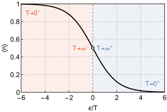
Figure 1: All physical single-mode fermionic states are thermal Gaussian states characterized by the Fermi-Dirac distribution $\braket{n}=1/(1+e^{\epsilon/T})$. The positive and negative temperatures are associated with the blue- and red-shaded regions, respectively. The vacuum $\ket{0}$ and excited state $\ket{1}$ are reached in the limit $T\to 0^{+}$ and $T\to 0^{-}$, respectively.

It is instructive to describe physical states in terms of the occupation number $\braket{n}=e^{\nu}/(e^{\nu}+1)=1/(1+e^{\epsilon/T})$, which corresponds to the Fermi-Dirac distribution (see Figure 1). Note first that the purity of (5) yields

$$\textbf{Tr}\{\bm{\rho}^{2}\}=1-2\braket{n}\left(1-\braket{n}\right),$$ (6)

implying that the only two pure states are the vacuum ($\braket{n}=0$) and excited state $(\braket{n}=1)$. The family of physical states can be divided into positive- and negative-temperature thermal states . The two branches are connected by the maximally-mixed state with $\braket{n}=1/2$, which requires an infinite temperature of arbitrary sign $T\to\infty^{\pm}$. The vacuum and excited states correspond to the zero-temperature limits $T\to 0^{+}$ and $T\to 0^{-}$, respectively. In this sense, they correspond to the extremal points of the set of physical states and we may expect their uncertainty in phase space to play a special role too.

Fermionic coherent states — Following [44], we introduce the fermionic displacement operator

$$\begin{split}\bm{D}(\alpha)&=e^{\bm{a}^{\dagger}\alpha-\alpha^{*}\bm{a}}\\ &=\mathds{1}+\bm{a}^{\dagger}\alpha-\alpha^{*}\bm{a}+\left({\scriptstyle\frac{1}{2}}\,\mathds{1}-\bm{a}^{\dagger}\bm{a}\right)\alpha\alpha^{*},\end{split}$$ (7)

with $\alpha,\alpha^{*}$ being Grassmann-valued variables such that

$$\begin{split}&\left\{\alpha,\alpha^{*}\right\}=\left\{\alpha,\alpha\right\}=\left\{\alpha^{*},\alpha^{*}\right\}=0,\end{split}$$ (8)

which also anticommute with the Grassmann-valued mode operators $\bm{a},\bm{a}^{\dagger}$, namely

$$\begin{split}&\left\{\alpha,\bm{a}\right\}=\left\{\alpha,\bm{a}^{\dagger}\right\}=\left\{\alpha^{*},\bm{a}\right\}=\left\{\alpha^{*},\bm{a}^{\dagger}\right\}=0.\end{split}$$ (9)

From Eq. (7), it is easy to check that $\bm{D}(\alpha)$ is a unitary operator and $\bm{D}^{\dagger}(\alpha)=\bm{D}(-\alpha)$. Then, fermionic coherent states are defined as displaced vacuum states

$$\ket{\alpha}=\bm{D}(\alpha)\ket{0},$$ (10)

with Grassmann-valued displacements $\alpha$. Although they are unphysical , the fermionic coherent states provide the right tool to express quasi-probability distributions in phase space. As in the bosonic case, the coherent state basis is overcomplete with the identity being represented as a Berezin integral , $\mathds{1}=\int\mathcal{D}\alpha\bm{\ket{\alpha}\bra{\alpha}}$ , where we have chosen the standard sign convention that the innermost integral is being performed first, i.e., $\int\mathcal{D}\alpha\,\alpha\alpha^{*}\equiv\int\mathrm{d}\alpha^{*}\mathrm{d}\alpha\,\alpha\alpha^{*}\equiv+1$. This also leads us to express the trace of an operator $\bm{O}$ in the coherent-state basis as

$$\textbf{Tr}\{\bm{O}\}=\int\mathcal{D}\alpha\braket{\alpha}{\bm{O}}{-\alpha}.$$ (11)

Note the discrepancy (minus sign) with the analog formula for bosonic coherent states .

Phase-space distributions and supernumbers — We are now ready to express the fermionic Wigner $W$- and Husimi $Q$-distributions. Just as their bosonic counterparts, the former is defined as the Fourier transform of the characteristic function $\chi(\alpha)=\textbf{Tr}\{\bm{\rho}\,\bm{D}(\alpha)\}$, namely

$$W(\alpha)=\int\mathcal{D}\beta\,e^{\alpha\beta^{*}-\beta\alpha^{*}}\,\chi(\beta),$$ (12)

while the latter is the outcome distribution obtained when measuring $\bm{\rho}$ in the coherent-state basis, namely

$$Q(\alpha)=\textbf{Tr}\{\bm{\rho}\bm{\ket{\alpha}\bra{\alpha}}\}=\braket{\alpha}{\bm{\rho}}{-\alpha}.$$ (13)

Both are Grassmann-even for physical states and can be computed analytically in full generality, which leads to the simple Gaussian expressions

$$\begin{split}W(\alpha)&=\left(1/2-\braket{n}\right)e^{\frac{\alpha\alpha^{*}}{1/2-\braket{n}}}=1/2-\braket{n}+\alpha\alpha^{*},\\ Q(\alpha)&=\left(1-\braket{n}\right)e^{\frac{\alpha\alpha^{*}}{1-\braket{n}}}=1-\braket{n}+\alpha\alpha^{*}.\end{split}$$ (14)

Since the prefactor of the term $\alpha\alpha^{*}$ is one in both cases, the phase-space distributions are normalized to unity with respect to the Berezin integral measure $\int\mathcal{D}\alpha\,W(\alpha)=\int\mathcal{D}\alpha\,Q(\alpha)=\textbf{Tr}\{\bm{\rho}\}=1$. Except for normalization, neither $W(\alpha)$ nor $Q(\alpha)$ has a straightforward physical interpretation (unlike their bosonic counterparts) since these are distributions over Grassmann variables.

To provide a deeper understanding of expressions (14), we make an excursion into the theory of supernumbers (see [64]). Every Grassmann number $z$, i.e., every element of the Grassmann algebra defined via (8), is a supernumber and can be decomposed linearly as $z=z_{\text{B}}+z_{\text{S}}$. Therein, the so-called body $z_{\text{B}}\in\mathbb{C}$ is the ordinary scalar part, while the so-called soul $z_{\text{S}}=c_{1}\alpha+c_{2}\alpha^{*}+c_{3}\alpha\alpha^{*}$ contains all Grassmann-valued contributions with complex-valued coefficients $c_{i}\in\mathbb{C}$. A supernumber $z$ is real if and only if $z^{*}=z$ and positive (negative) if and only if its body $z_{\text{B}}$ is positive (negative). The latter implies a partial order for supernumbers, namely that $z_{1}\leq z_{2}$ if and only if $z_{1,\text{B}}\leq z_{2,\text{B}}$ and vice versa.

Thus, the two phase-space distributions in (14) are real and have equal (Grassmann-even) souls $W_{\text{S}}=Q_{\text{S}}=\alpha\alpha^{*}$, but different bodies $W_{\text{B}}=1/2-\braket{n}$, $Q_{\text{B}}=1-\braket{n}$. Hence, the Husimi $Q$-distribution is always larger than the Wigner $W$-distribution, i.e., $Q(\alpha)>W(\alpha)$ for all $\alpha$ and $\braket{n}$, a relation which does not exist in the bosonic case. Further, the Husimi $Q$-distribution is always positive since $Q_{\text{B}}\geq 0$ for all $\braket{n}$, while the Wigner $W$-distribution is entirely positive (or entirely negative) for $0\leq\braket{n}<1/2$ (or for $1/2<\braket{n}\leq 1$), for which we write $W^{+}$ and $W^{-}$, respectively .

Majorization relations — We generalize the definition of a majorization relation for a bosonic mode (see [66, 35]) in a straightforward way: A phase-space distribution $z_{1}(\alpha)$ is said to be majorized by another distribution $z_{2}(\alpha)$, written as $z_{1}\prec z_{2}$, if and only if

$$\int\mathcal{D}\alpha\,f(z_{1})\geq\int\mathcal{D}\alpha\,f(z_{2}),$$ (15)

for all concave functions $f:\mathcal{I}(z_{\text{B}})\to\mathbb{R}$ with $f(0)=0$, where $\mathcal{I}(z_{\text{B}})\subset\mathbb{R}$ denotes the image of $z_{\text{B}}=z_{\text{B}}(\braket{n})$ . For the two phase-space distributions of interest, we shall prove the two fundamental majorization relations (here the index of $W$ or $Q$ refers to the value of $\braket{n}$):

1. Any Wigner $W$-distribution is majorized by (majorizes) the vacuum (excited) state, with the maximally-mixed state being majorized by (being majorizing) all Wigner-positive (-negative) distributions:

   $$W_{1}\prec W^{-}\prec W_{1/2}\prec W^{+}\prec W_{0}.$$ (16)

2. Any Husimi $Q$-distribution is majorized by (majorizes) the vacuum (excited) state:

   $$Q_{1}\prec Q\prec Q_{0}.$$ (17)

We stress that the right-hand sides of Eqs. (16) and (17) resemble the bosonic phase-space majorization conjecture [35] and the Lieb-Solovej theorem [32, 33, 34], respectively.

Their proofs rely on the central observation that concave averages in the fermionic phase space are real numbers, which can be computed explicitly for all phase-space distributions $z=W^{+},W^{-},Q$ of interest. To show this, we use the notion of an analytic functional over a supernumber $z=z_{\text{B}}+z_{\text{S}}$ via its Taylor expansion [64]

$$f(z)=\sum_{j=0}^{\infty}\frac{1}{j!}\,f^{(j)}(z_{\text{B}})\,z_{\text{S}}^{j},$$ (18)

where $f^{(j)}(z_{\text{B}})$ denotes the $j$th derivative of $f$ evaluated at the body $z_{\text{B}}$. Using that the soul of all physical phase-space distributions (14) is nilpotent, i.e., $z_{\text{S}}^{j}=(\alpha\alpha^{*})^{j}=0$ for all $j>1$, immediately implies

$$\int\mathcal{D}\alpha\,f(z)=\int\mathcal{D}\alpha\,\left[f(z_{\text{B}})+f^{\prime}(z_{\text{B}})\alpha\alpha^{*}\right]=f^{\prime}(z_{\text{B}}).$$ (19)

Since $f$ is concave, its first derivative is a monotonically decreasing function, i.e.,

$$t_{1}\leq t_{2}\Rightarrow f^{\prime}(t_{1})\geq f^{\prime}(t_{2}),$$ (20)

for all $t_{1},t_{2}\in\mathcal{I}$. Hence, if two phase-space distributions $z_{1}(\alpha)$ and $z_{2}(\alpha)$ satisfy $z_{1,\text{B}}\leq z_{2,\text{B}}$, then, using (15) and (19), the fermionic phase-space majorization relation $z_{1}\prec z_{2}$ must hold. Thus, these majorization relations are ultimately a consequence of the image of $z_{\text{B}}$ being bounded. More precisely, $-1/2\leq\mathcal{I}(W^{-}_{\text{B}})\leq 0\leq\mathcal{I}(W^{+}_{\text{B}})\leq 1/2$ implies $f^{\prime}(-1/2)\geq f^{\prime}(W^{-}_{\text{B}})\geq f^{\prime}(0)\geq f^{\prime}(W^{+}_{\text{B}})\geq f^{\prime}(1/2)$, which in turn implies (16). Analogously, $0\leq\mathcal{I}(Q_{\text{B}})\leq 1$ implies $f^{\prime}(0)\geq f^{\prime}(Q_{\text{B}})\geq f^{\prime}(1)$, from which (17) follows.

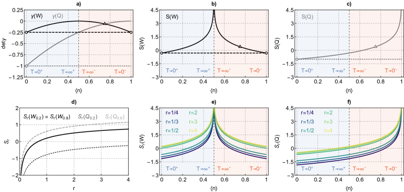
Figure 2: Measures of disorder in fermionic phase-space and their lower bounds expressing the uncertainty principle as functions of the particle number $\braket{n}$. a) shows the two second-moment measures $\det\gamma(W)$ (black) and $\det\gamma(Q)$ (gray), while b) and c) contain their entropic analogs, respectively. The curves for the $W$- and $Q$-distributions intersect at $\braket{n}=3/4$ (triangle). The extension to Rényi entropies for various entropic orders is presented in e) and f). From d) we observe $S_{r}(W_{\braket{n}})=S_{r}(W_{1-\braket{n}})$, $S_{r}(W_{\braket{n}})>(<)S_{r}(Q_{\braket{n}})$ for $\braket{n}<(>)\,3/4$ and that $S_{r}(z)$ is monotonically increasing in $r$.

Second-moment uncertainty relations — We consider now the fermionic covariance matrix associated with the phase-space distribution $z(\alpha)$, which we define as

$$\gamma_{jj^{\prime}}(z)\equiv\frac{1}{2i}\int\mathcal{D}\alpha\,z(\alpha)\,[\alpha_{j},\alpha_{j^{\prime}}]=z_{\text{B}}\,(\sigma_{y})_{jj^{\prime}},$$ (21)

with $j,j^{\prime}=1,2$ (we set $\alpha_{1}\equiv\alpha$ and $\alpha_{2}\equiv\alpha^{*}$) and $\sigma_{y}$ being the second Pauli matrix . Its determinant

$$\det\gamma(z)=-z_{\text{B}}^{2}$$ (22)

is non-trivially bounded from below by the uncertainty principle (just as for a bosonic mode). Indeed, the determinants of the covariance matrix of the Wigner $W$- and Husimi $Q$-distributions read

$$\begin{split}\det\gamma(W)&=-(1/2-\braket{n})^{2},\\ \det\gamma(Q)&=-(1-\braket{n})^{2},\end{split}$$ (23)

so we have the second-moment uncertainty relations

$$\begin{split}\det\gamma(W_{1/2})&\geq\det\gamma(W)\geq\det\gamma(W_{\{0,1\}})=-1/4,\\ \det\gamma(Q_{1})&\geq\det\gamma(Q)\geq\det\gamma(Q_{0})=-1,\end{split}$$ (24)

respectively. The two determinants and their bounds are shown in Figure 2 a). Interestingly, $\det\gamma(W)\geq-1/4$ and $\det\gamma(Q)\geq-1$ resemble the Robertson-Schrödinger uncertainty relation and the uncertainty relation presented in [23], respectively, up to an overall minus sign. Note also that $\det\gamma(W)\geq-1/4$ is a simple consequence of Pauli’s principle, implying that $\braket{n}$ must belong to $[0,1]$

Entropic uncertainty relations — We define the Rényi entropy of a fermionic phase-space distribution $z(\alpha)$ with possibly negative body $z_{\text{B}}$ as

$$\begin{split}S_{r}(z)&\equiv\frac{1}{1-r}\ln\int\mathcal{D}\alpha\,\lvert z(\alpha)\rvert^{r},\end{split}$$ (25)

where $r\in(0,1)\cup(1,\infty)$ denotes the entropic order. The Shannon entropy $S(z)\equiv-\int\mathcal{D}\alpha\,z(\alpha)\ln z(\alpha)$ is recovered in the limit $r\to 1$. For $z_{\text{B}}\geq 0$, (25) reduces to the standard definition, while for $z_{\text{B}}<0$, $h_{r}(z)$ is basically defined as the standard Rényi entropy of $-z>0$. Further, (25) is concave in $z$ over the whole set of states when $r>1$ and for $0<r<1$ when considering only Wigner-positive or Wigner-negative states .

Following (19) (or by using the nilpotency of $z_{\text{S}}$), we have that $\int\mathcal{D}\alpha\,\lvert z(\alpha)\rvert^{r}=r\lvert z_{\text{B}}\rvert^{r-1}$, which allows to evaluate the Rényi entropy of the Wigner $W$- and Husimi $Q$-distributions explicitly as

$$\begin{split}S_{r}(W)&=\frac{\ln r}{1-r}-\ln\big{|}1/2-\braket{n}\big{|},\\ S_{r}(Q)&=\frac{\ln r}{1-r}-\ln\left(1-\braket{n}\right).\end{split}$$ (26)

Therefore, the entropic uncertainty relations in fermionic phase space are written as

$$\begin{split}S_{r}(W)&\geq S_{r}(W_{\{0,1\}})=\frac{\ln r}{1-r}+\ln 2,\\ S_{r}(Q)&\geq S_{r}(Q_{0})=\frac{\ln r}{1-r}.\end{split}$$ (27)

We analyze these entropies and their bounds in Figure 2 b) - f). When taking the limit $r\to 1$, the two uncertainty relations $S(W)\geq-1+\ln 2$ and $S(Q)\geq-1$ resemble the bosonic Wigner entropy conjecture for Wigner-positive states [17] and the Wehrl-Lieb inequality [72, 73, 74], respectively, except for a minus sign . However, we also observe two significant differences to the bosonic case: First, the family of fermionic Rényi entropies is monotonically increasing (instead of decreasing) in the entropic order $r$, see the lower row in Figure 2. Second, the uncertainty encoded in the Wigner $W$-distribution is larger (or smaller) than the one encoded in the Husimi $Q$-distribution for $\braket{n}<(\mathrm{or}>)\,3/4$ for all measures (see white triangles at $\braket{n}=3/4$ in the upper row of Figure 2).

Discussion — We have derived fermionic uncertainty relations, Eqs. (24) and (27), as well as fermionic majorization relations, Eqs. (16) and (17). These relations are fundamentally implied by Pauli’s principle, which states that the vacuum (excited) state has the lowest (highest) occupation. Since all physical states of a single fermionic mode are Gaussian, the moment-based, entropy-based, and majorization-based uncertainty relations are all equivalent (for a given phase-space distribution $z$). First, it is simple to see that $S_{r}(z)=\ln r/(1-r)-(1/2)\ln[-\det\gamma(z)]$ for all Gaussian $z$, hence (24) and (27) are equivalent. Second, the equivalence between (24) and (16), (17) is a consequence of the behavior of the majorization relation (15) under a change of Grassmann-valued variable . The Gaussian nature of $z$ is the key feature enabling our exact derivation here, in sharp contrast with bosonic uncertainty relations and majorization relations, which remain hard problems.

With our analysis we have paved the ground for applying the uncertainty principle to quantum information problems for fermionic systems, e.g., in the context of entanglement theory or quantum cryptography. Although the fermionic phase-space distributions are themselves Grassmann-valued, all measures of disorder such as the entropy are real-valued and, even more importantly, measurable as they can be computed from the occupation numbers of the system. On the theoretical side, it is of particular interest to extend our fermionic uncertainty relations to arbitrary many modes [19], where the set of physical states also contains non-Gaussian states, presumably leading to a hierarchy of uncertainty relations more comparable to the bosonic case.

Acknowledgements — We thank Zacharie Van Herstraeten for useful discussions on the subject. We acknowledge support from the European Union under project ShoQC within ERA-NET Cofund in Quantum Technologies (QuantERA) program, as well as from the F.R.S.-FNRS under project CHEQS under the Excellence of Science (EOS) program.

References

- Heisenberg [1927] W. Heisenberg, Über den anschaulichen Inhalt der quantentheoretischen Kinematik und Mechanik, Z. Phys. 43, 172 (1927).
- Kennard [1927] E. H. Kennard, Zur Quantenmechanik einfacher Bewegungs-typen, Z. Phys. 44, 326 (1927).
- Robertson [1929] H. P. Robertson, The Uncertainty Principle, Phys. Rev. 34, 163 (1929).
- Robertson [1930] H. P. Robertson, A general formulation of the uncertainty principle and its classical interpretation, Phys. Rev. 35, 667 (1930).
- Schrödinger [1930] E. Schrödinger, Zum Heisenbergschen Unschärfeprinzip, Sitzungsberichte der Preußischen Akademie der Wissenschaften. Physikalisch-mathematische Klasse 14, 296 (1930).
- Everett [1957] H. Everett, ’Relative State’ Formulation of Quantum Mechanics, Rev. Mod. Phys. 29, 454 (1957).
- Beckner [1975] W. Beckner, Inequalities in Fourier Analysis, Ann. Math. 102, 159 (1975).
- Deutsch [1983] D. Deutsch, Uncertainty in Quantum Measurements, Phys. Rev. Lett. 50, 631 (1983).
- Kraus [1987] K. Kraus, Complementary observables and uncertainty relations, Phys. Rev. D 35, 3070 (1987).
- Maassen and Uffink [1988] H. Maassen and J. B. M. Uffink, Generalized entropic uncertainty relations, Phys. Rev. Lett. 60, 1103 (1988).
- Berta et al. [2010] M. Berta, M. Christandl, R. Colbeck, J. M. Renes, and R. Renner, The uncertainty principle in the presence of quantum memory, Nat. Phys. 6, 659 (2010).
- Wehner and Winter [2010] S. Wehner and A. Winter, Entropic uncertainty relations—a survey, New J. Phys. 12, 025009 (2010).
- Coles et al. [2012] P. J. Coles, R. Colbeck, L. Yu, and M. Zwolak, Uncertainty Relations from Simple Entropic Properties, Phys. Rev. Lett. 108, 210405 (2012).
- Białynicki-Birula and Mycielski [1975] I. Białynicki-Birula and J. Mycielski, Uncertainty relations for information entropy in wave mechanics, Commun. Math. Phys. 44, 129 (1975).
- Frank and Lieb [2012] R. L. Frank and E. H. Lieb, Entropy and the Uncertainty Principle, Ann. Henri Poincaré 13, 1711 (2012).
- Hertz and Cerf [2019] A. Hertz and N. J. Cerf, Continuous-variable entropic uncertainty relations, J. Phys. A Math. Theor. 52, 173001 (2019).
- Van Herstraeten and Cerf [2021] Z. Van Herstraeten and N. J. Cerf, Quantum Wigner entropy, Phys. Rev. A 104, 042211 (2021).
- Floerchinger et al. [2022a] S. Floerchinger, T. Haas, and M. Schröfl, Relative entropic uncertainty relation for scalar quantum fields, SciPost Phys. 12, 089 (2022a).
- Ditsch and Haas [2023] S. Ditsch and T. Haas, Entropic distinguishability of quantum fields in phase space, arXiv:2307.06128 (2023).
- Walborn et al. [2009] S. P. Walborn, B. G. Taketani, A. Salles, F. Toscano, and R. L. de Matos Filho, Entropic Entanglement Criteria for Continuous Variables, Phys. Rev. Lett. 103, 160505 (2009).
- Saboia et al. [2011] A. Saboia, F. Toscano, and S. P. Walborn, Family of continuous-variable entanglement criteria using general entropy functions, Phys. Rev. A 83, 032307 (2011).
- Schneeloch et al. [2019] J. Schneeloch, C. C. Tison, M. L. Fanto, P. M. Alsing, and G. A. Howland, Quantifying entanglement in a 68-billion-dimensional quantum state space, Nat. Commun. 10, 1 (2019).
- Floerchinger et al. [2021] S. Floerchinger, T. Haas, and H. Müller-Groeling, Wehrl entropy, entropic uncertainty relations, and entanglement, Phys. Rev. A 103, 062222 (2021).
- Floerchinger et al. [2022b] S. Floerchinger, M. Gärttner, T. Haas, and O. R. Stockdale, Entropic entanglement criteria in phase space, Phys. Rev. A 105, 012409 (2022b).
- Grosshans and Cerf [2004] F. Grosshans and N. J. Cerf, Continuous-Variable Quantum Cryptography is Secure against Non-Gaussian Attacks, Phys. Rev. Lett. 92, 047905 (2004).
- Renes and Boileau [2009] J. M. Renes and J.-C. Boileau, Conjectured Strong Complementary Information Tradeoff, Phys. Rev. Lett. 103, 020402 (2009).
- Tomamichel and Renner [2011] M. Tomamichel and R. Renner, Uncertainty Relation for Smooth Entropies, Phys. Rev. Lett. 106, 110506 (2011).
- Furrer et al. [2012] F. Furrer, T. Franz, M. Berta, A. Leverrier, V. B. Scholz, M. Tomamichel, and R. F. Werner, Continuous Variable Quantum Key Distribution: Finite-Key Analysis of Composable Security against Coherent Attacks, Phys. Rev. Lett. 109, 100502 (2012).
- Tomamichel et al. [2012] M. Tomamichel, C. C. W. Lim, N. Gisin, and R. Renner, Tight finite-key analysis for quantum cryptography, Nat. Comm. 3, 634 (2012).
- Partovi [2011] M. H. Partovi, Majorization formulation of uncertainty in quantum mechanics, Phys. Rev. A 84, 052117 (2011).
- Narasimhachar et al. [2016] V. Narasimhachar, A. Poostindouz, and G. Gour, Uncertainty, joint uncertainty, and the quantum uncertainty principle, New J. Phys. 18, 033019 (2016).
- Lieb and Solovej [2014] E. H. Lieb and J. P. Solovej, Proof of an entropy conjecture for Bloch coherent spin states and its generalizations, Acta Math. 212, 379 (2014).
- Lieb and Solovej [2016] E. H. Lieb and J. P. Solovej, Proof of the Wehrl-type Entropy Conjecture for Symmetric Coherent States, Commun. Math. Phys. 348, 567 (2016).
- Lieb and Solovej [2021] E. H. Lieb and J. P. Solovej, Wehrl-type coherent state entropy inequalities for SU(1,1) and its AX+B subgroup, in Partial Differential Equations, Spectral Theory, and Mathematical Physics (2021) p. 301–314.
- Van Herstraeten et al. [2023] Z. Van Herstraeten, M. G. Jabbour, and N. J. Cerf, Continuous majorization in quantum phase space, Quantum 7, 1021 (2023).
- Nielsen [1999] M. A. Nielsen, Conditions for a Class of Entanglement Transformations, Phys. Rev. Lett. 83, 436 (1999).
- Gärttner et al. [2023a] M. Gärttner, T. Haas, and J. Noll, General Class of Continuous Variable Entanglement Criteria, Phys. Rev. Lett. 131, 150201 (2023a).
- Gärttner et al. [2023b] M. Gärttner, T. Haas, and J. Noll, Detecting continuous-variable entanglement in phase space with the distribution, Phys. Rev. A 108, 042410 (2023b).
- Weedbrook et al. [2012] C. Weedbrook, S. Pirandola, R. García-Patrón, N. J. Cerf, T. C. Ralph, J. H. Shapiro, and S. Lloyd, Gaussian quantum information, Rev. Mod. Phys. 84, 621 (2012).
- Serafini [2017] A. Serafini, Quantum Continuous Variables (CRC Press, 2017).
- Nielsen and Chuang [2010] M. A. Nielsen and I. L. Chuang, Quantum Computation and Quantum Information: 10th Anniversary Edition (Cambridge University Press, 2010).
- Wilde [2013] M. M. Wilde, Quantum Information Theory (Cambridge University Press, 2013).
- Pauli [1925] W. Pauli, Über den Zusammenhang des Abschlusses der Elektronengruppen im Atom mit der Komplexstruktur der Spektren, Z. Physik 31, 765 (1925).
- Cahill and Glauber [1999] K. E. Cahill and R. J. Glauber, Density operators for fermions, Phys. Rev. A 59, 1538 (1999).
- Hackl and Bianchi [2021] L. Hackl and E. Bianchi, Bosonic and fermionic Gaussian states from Kähler structures, SciPost Phys. Core 4, 025 (2021).
- Bañuls et al. [2007] M.-C. Bañuls, J. I. Cirac, and M. M. Wolf, Entanglement in fermionic systems, Phys. Rev. A 76, 022311 (2007).
- Zander and Plastino [2010] C. Zander and A. R. Plastino, Uncertainty relations and entanglement in fermion systems, Phys. Rev. A 81, 062128 (2010).
- Friis et al. [2013] N. Friis, A. R. Lee, and D. E. Bruschi, Fermionic-mode entanglement in quantum information, Phys. Rev. A 87, 022338 (2013).
- Friis [2016] N. Friis, Reasonable fermionic quantum information theories require relativity, New J. Phys. 18, 033014 (2016).
- Casini and Huerta [2009] H. Casini and M. Huerta, Entanglement entropy in free quantum field theory, J. Phys. A Math. Theo. 42, 504007 (2009).
- Calabrese and Cardy [2004] P. Calabrese and J. Cardy, Entanglement entropy and quantum field theory, J. Stat. Mech. Theo. Exp. 2004, P06002 (2004).
- Calabrese and Cardy [2009] P. Calabrese and J. Cardy, Entanglement entropy and conformal field theory, J. Phys. A Math. Theo. 42, 504005 (2009).
- Hegerfeldt et al. [1968] G. C. Hegerfeldt, K. Kraus, and E. P. Wigner, Proof of the Fermion Superselection Rule without the Assumption of Time-Reversal Invariance, J. Math. Phys. 9, 2029 (1968).
- Note [1] For , the state (4\@@italiccorr) is still Gaussian, i.e. can can be written .
- Note [2] Negative temperatures can occur for a Hamiltonian bounded from above when the occupation of the excited states is more likely. In our case, this amounts to .
- Note [3] We note that fermionic coherent states are unphysical unless , see also [45]. Indeed, from Eq. (7\@@italiccorr), we see that they are superpositions . In analogy to the bosonic case, fermionic coherent states are eigenstates of the annihilation operator .
- Note [4] Berezin integrals are integrals over Grassmann-valued variables, which are such that and , showing that integration is equivalent to differentiation for Grassmann variables. The Berezin integral of any other function is immediate since higher-order powers with vanish for a Grassmann variable .
- Note [5] This decomposition of the identity in terms of fermionic coherent states can be checked by using and , with , together with the fact that as well as given is Grassmann-valued.
- Note [6] This expression for the trace in the fermionic coherent basis can be checked by using and , with , together with the fact that as well as given is Grassmann-valued.
- Note [7] We may easily verify that the minus sign in is needed by applying Eq. (11\@@italiccorr) to the density operator . Indeed, we get whereas we would get by (wrongly) replacing with , so that the excited state would be (wrongly) normalized to . This issue is intrinsically linked to the fact that and anticommute for (whereas they commute for ), so we have to insert this minus sign when exchanging the two matrix elements (this works both for and ).
- Note [8] Note again the minus sign in Eq. (13\@@italiccorr), which strikingly contrasts with the analog formula for a bosonic mode and is directly connected to the negative sign in Eq. (11\@@italiccorr).
- Note [9] We argue that any physical quantity has to be of definite Grassmann-parity, that is, either fully commute or anti-commute with any Grassmann variable, which we refer to as Grassmann-even or Grassmann-odd, respectively (see also [44]).
- Note [10] Using as well as , the characteristic function of can be expressed as . To obtain , we perform the Fourier transform of by exploiting the identity and remembering that and are Grassmann variables. The expression of is also straightforward to derive by using the expansion of and in the Fock basis.
- DeWitt [1992] B. DeWitt, Supermanifolds, 2nd ed., Cambridge Monographs on Mathematical Physics (Cambridge University Press, 1992).
- Note [11] We note that in contrast to the bosonic case, where a complete characterization of the set of Wigner-positive states is an outstanding problem, the sign of the single-mode fermionic Wigner -distribution is fully determined by the particle number .
- Marshall et al. [2011] A. W. Marshall, I. Olkin, and B. C. Arnold, Inequalities: Theory of Majorization and Its Applications (Springer New York, 2011).
- Note [12] Without the condition both sides of the majorization relation would diverge.
- Note [13] Since all higher derivatives of are multiplied by zero, we do not even have to assume that is analytic. Further, the existence of its first derivative is guaranteed almost everywhere following Rademacher’s theorem for Lipschitz-continuous functions with the only exceptions occurring at the boundary points.
- Note [14] Note that physical states are Gaussian states that are centered at the origin, i.e., , hence the second-order moments are centered moments.
- Note [15] Continuous-variable entropies of classical probability distributions are commonly denoted by , but we choose the convention that is preferred in the mathematical literature, see e.g., [72, 73, 74, 32, 77].
- Note [16] For the latter two arguments note again that any Wigner -distribution is either entirely positive or negative.
- Wehrl [1978] A. Wehrl, General properties of entropy, Rev. Mod. Phys. 50, 221 (1978).
- Wehrl [1979] A. Wehrl, On the relation between classical and quantum-mechanical entropy, Rep. Math. Phys. 16, 353 (1979).
- Lieb [1978] E. H. Lieb, Proof of an entropy conjecture of Wehrl, Commun. Math. Phys. 62, 35 (1978).
- Note [17] For comparison, the corresponding inequalities for a bosonic mode read and . Note that the fermionic Wigner -distribution comes without the normalization factor of that prevails in the bosonic case, see Eq. (12\@@italiccorr). Hence, mimicking the fermionic normalization would decrease the bosonic Wigner entropy by , so the corrected bosonic lower bound would read , which is exactly the fermionic lower bound with a minus sign. For the Husimi -distribution, the bosonic and fermionic lower bounds are also the same, up to a minus sign.
- Note [18] We note that any physical distributions is related to another distribution by such that , where is a real number. Then, the majorization relation (15\@@italiccorr) can be rewritten as . (Note here that a change of coordinates for Grassmann variables is accompanied by the inverse Jacobian.) Since is concave and fulfills , it is subadditive, and thus the latter relation is fulfilled if which implies when . The converse statement follows from transforming the left-hand side of (15\@@italiccorr) instead.
- Schupp [2022] P. Schupp, Wehrl entropy, coherent states and quantum channels, in The Physics and Mathematics of Elliott Lieb (EMS Press, 2022) pp. 329–344.