Quantum information scrambling in two-dimensional Bose-Hubbard lattices

Abstract

It is a well-understood fact that the transport of excitations throughout a lattice is intimately governed by the underlying structures. Hence, it is only natural to recognize that also the dispersion of information has to depend on the lattice geometry. In the present work, we demonstrate that two-dimensional lattices described by the Bose-Hubbard model exhibit information scrambling for systems as little as two hexagons. However, we also find that the OTOC shows the exponential decay characteristic for quantum chaos only for a judicious choice of local observables. More generally, the OTOC is better described by Gaussian-exponential convolutions, which alludes to the close similarity of information scrambling and decoherence theory.

I Introduction

In India they call it Akuri or Bhurji, and in the Spanish speaking world it is Revuelto – yet all of these terms refer rather literally to one of the most common breakfast items, namely scrambled eggs [1]. Nowadays it has become a typical marketing strategy to embellish pretty much any product name with the attribute ”quantum”, and even “quantum eggs” have become a phenomenon of popular culture [2, 3].

Yet, quantum information scrambling [4] is an actual scientific term that refers to the spread of initially localized quantum information throughout non-local degrees of freedom in complex many body systems [5, 6, 7, 8, 9, 10]. Arguably, the most commonly used quantifier for the rate with which information becomes non-local is the Out-of-Time-Ordered Correlator (OTOC) [11, 12, 13, 14, 15, 16, 17, 18]. In particular, an exponential scaling of the OTOC as a function of time signifies quantumly chaotic dynamics [19, 20, 14], with corresponding quantum Lyapunov exponents [21, 22, 23].

In recent years, quantum information scrambling has attracted significant interest, see for instance a recent perspective [4] and references therein. However, a comprehensive analysis of the dynamics of complex many body systems typically requires sophisticated numerical tools. Hence, a large fraction of the literature has focused on systems with effectively one-dimensional geometry, such as the disordered XXX chain [24] or the mixed-field Ising model [25, 26]. Note that paradigmatic examples of fast scramblers are built from Sachdev-Ye-Kitaev (SYK) models [27, 28, 29, 30], which, however, do not have a clear notion of dimensionality due to their full connectivity.

In the present work, we study the dynamics of information scrambling in lattices with two-dimensional geometry. As a Hamiltonian, we choose the Bose-Hubbard model, for which chaotic behavior has been reported [31, 32]. Note that the Bose-Hubbard Model undergoes a second order quantum phase transition from the superfluid phase to the Mott insulator phase [33, 34, 35, 36, 18]. The quantum critical region is strongly interacting, and the energy conserving interactions between the quasi particles in this regime are responsible for the thermalization of the system at strong couplings [37, 18]. Interestingly, it was found in Ref. [32] that the dynamics is quantum chaotic at strong couplings and that the Lyapunov exponent displays a maximum around the quantum critical region. Moreover, the eigenvalue statistics, excessive kurtosis of eigenstates, and the eigenstate thermalisation hypothesis have been analyzed [38].

What makes the Bose-Hubbard model particularly interesting is the fact that in hexagonal lattices the two-dimensional system exhibits Dirac points in the energy bands, which describes the motion of effectively relativistic dynamics [39]. It appears plausible that the dispersion relation governs the rate with which information can be scrambled, and hence it is only natural to study the effect of the lattice geometry on the dynamics of the OTOC in scrambling systems. Indeed, we find that in two-dimensional lattices, the OTOC is sensitive to the neighborhood of support of initial local operators, and that it displays a transition from Gaussian to near exponential decay as we change the configuration of the lattices and/or increase their sizes. Interestingly, when using the OTOC as a scrambling quantifier, it has been argued that decoherence and scrambling dynamics are hardly distinguishable in open systems [5, 40]. This is further supported by our current findings, as the OTOC is, indeed, best described by a convolution of Gaussian and exponential function, which is in full analogy to the decoherence factor [41].

II Preliminaries

We start by establishing notions and notations, and specifying the model.

II.1 The Bose-Hubbard model

The Hubbard model was originally developed to describe strongly-correlated electrons in solids [42]. As such, creation and annihilation operators were equipped with the fermionic commutation relation. Yet, also the corresponding bosonic version has found widespread applications, in for instance describing optical lattices [43].

The Hamiltonian is usually written as

$$H=-J\sum_{\langle i,j\rangle}\left(a_{i}^{\dagger}a_{j}+a_{j}^{\dagger}a_{i}\right)+\frac{U}{2}\sum_{i}n_{i}\left(n_{i}-1\right)$$ (1)

where $J$ is the hopping coefficient, $U$ is the on-site potential and $n_{i}=a_{i}^{\dagger}a_{i}$ describes the number of bosons at site $i$. Note that the lattice geometry is entirely encoded in the first sum.

The Bose-Hubbard model exhibits a quantum phase transition. When the first term in Eq. (1) is dominant, then the bosons can freely hop from one site to another and thus condense into a superfluid phase. On the other hand, when the second term is dominant, then the bosons have to pay a high potential cost to condense into a single site, and thus they prefer to stay at their respective sites resulting in a Mott insulator state. This transition was observed in ultracold atoms in optical lattices [44], and it has been demonstrated that the behavior around the critical point is well-described by the Kibble-Zurek mechanism [45, 35, 46, 47].

In the following analysis, we will study the dynamics of spreading information through different lattice geometries. As a main diagnostics tool, we will be using the OTOC. For a brief discussion of other quantifiers of scrambling, we refer to Appendix A.

II.2 Quantifying scrambling – the OTOC

In classical Hamiltonian dynamics, chaos can be identified from the exponential growth of the Poisson bracket [48]. Hence, arguably the most prominent tool to diagnose scrambling of quantum information is a closely related quantity – the OTOC [13].

The OTOC is a four-point correlation function that measures the growth of operators in the Heisenberg picture, and it can be written as

$$\text{OTOC}(t)=\left\langle\psi\right|A^{\dagger}(t)B^{\dagger}A(t)B\left|\psi\right\rangle$$ (2)

where $A,B$ are two local operators, $A(t)=\exp{(iHt)}A\exp{(-iHt)}$ is the time evolved operator in the Heisenberg picture and $H$ is the Hamiltonian describing the system of interest. Moreover, $\left|\psi\right\rangle$ is an initial state of the system. Since $A$ and $B$ are initially local operators, usually defined at two different sites on a lattice, they commute with each other. However, with time, $A(t)$ develops support on other sites in the lattice and as a result $[A(t),B]\neq 0$.

It is easy to see that at $t=0$ we simply have $\text{OTOC}(0)=1$, and that for $t>0$ we observe $\text{OTOC}(t)<1$. For spatial systems, we can associate a velocity with the OTOC, called the butterfly velocity [20, 49]. This velocity characterises local operators’ growth in time. For non-relativistic lattices, the Lieb-Robinson velocity places an upper bound on the size of time-evolved operators and is state independent [50, 51, 52]. It has been shown that the butterfly velocity is an effective state-dependent Lieb-Robinson velocity [53].

III Scrambling in 2D

To analyze the scrambling properties of the Bose-Hubbard model, we solved the ensuing dynamics numerically. To this end, we used Krylov subspace methods [54] to compute the time evolution operator. For the present purposes, we chose the following OTOC

$$\text{OTOC}(t)=\langle a_{j}^{\dagger}(t)a_{i}^{\dagger}a_{j}(t)a_{i}\rangle_{\psi}$$ (3)

where $i$ and $j$ are a pair of specific sites in the lattice, and the initial state is chosen to be all-up, $\psi=\left|1,1,1,\dots\right\rangle$. In Appendix A we briefly present results for one-dimensional lattices with periodic boundary conditions. For a lattice with 6 sites and 6 bosons, we observe convincing evidence of scrambling in the superfluid phase.

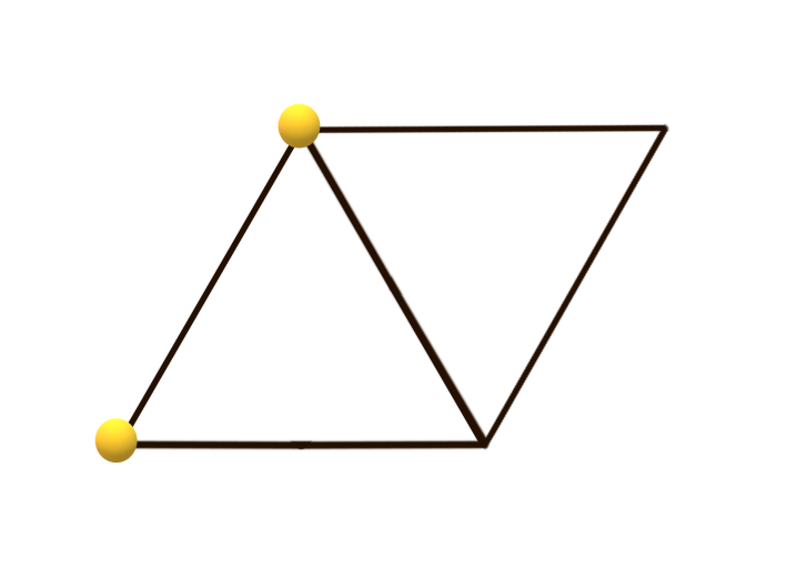
(a) Configuration 1

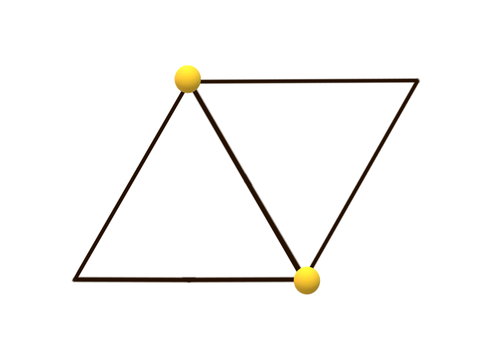
(b) Configuration 2

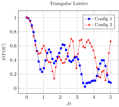
Figure 1: OTOC (3) as function of $Jt$, for two configurations of the triangular lattice for $U/J=4$ and $J=4$.

III.1 Triangular and square geometries

We start with the simplest two-dimensional geometries, before systematically building up to hexagonal geometries.

Triangular unit cell

In Fig. 1 we plot the OTOC (3) for a small lattice comprising two triangles. We observe a rapid decay of the OTOC, followed by sizable fluctuations. This evidences the small system size, which makes an analysis of universal properties of the dynamics inconclusive.

Square unit cell

We continue with the next simplest geometry, namely a finite lattice comprised of two squares. The corresponding results are depicted in Fig. 2. We observe qualitatively the same behavior as for the triangular cases. Note, however, that the fluctuations from the finite-size effects are significantly less pronounced.

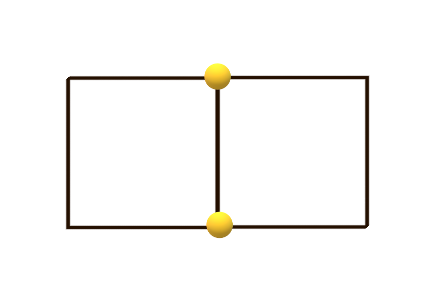
(a) Configuration 1

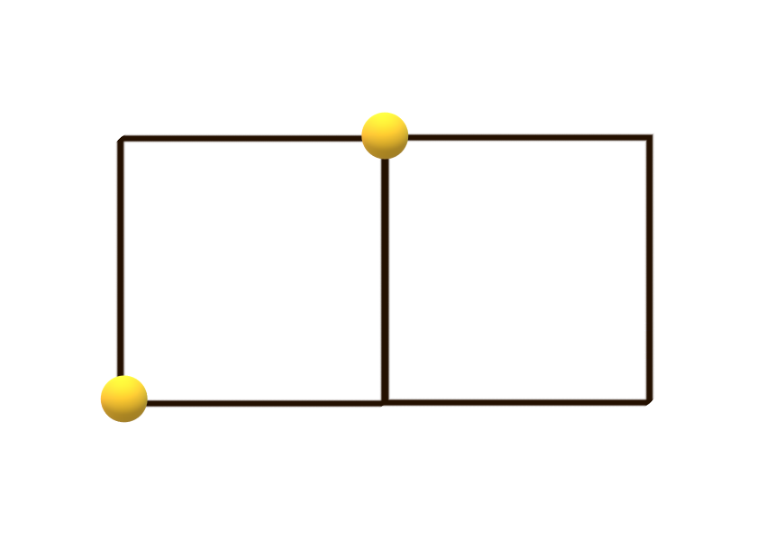
(b) Configuration 2

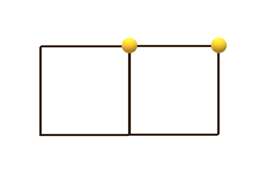
(c) Configuration 3

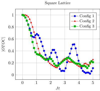
Figure 2: OTOC (3) as function of $Jt$, for three configurations of the square lattice for $U/J=4$ and $J=4$..

Triangular-square unit cell

As a final example, before moving on to hexagonal geometries, we consider a mixed case. In Fig. 3 we summarize findings for lattice configurations that are comprised of a triangle and a square. We find that the increased complexity of the geometry does not lead to qualitatively different behavior, but rather that the dynamics is still governed by finite size effects. In fact, the irregular fluctuations of the OTOC are more pronounced than for the regular square configurations in Fig. 2.

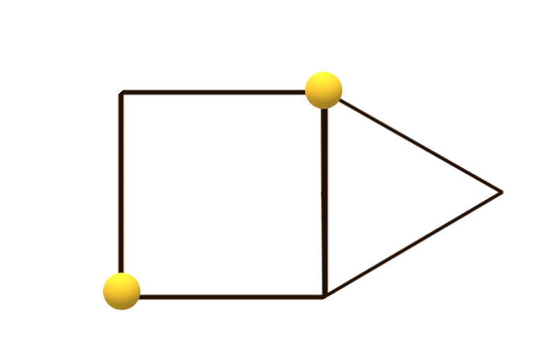
(a) Configuration 1

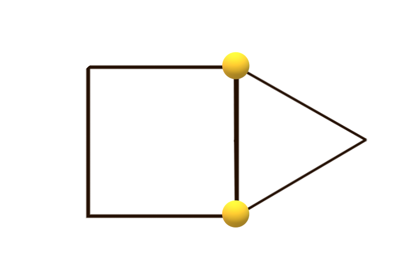
(b) Configuration 2

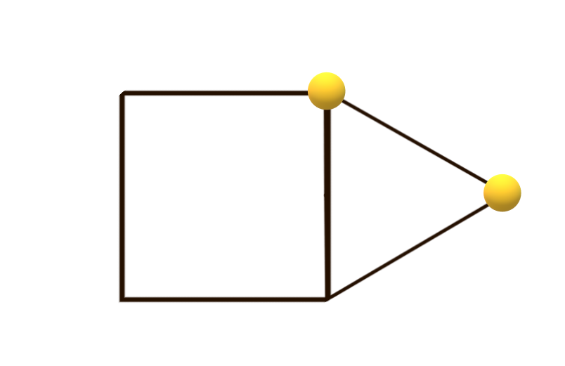
(c) Configuration 3

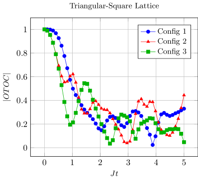
Figure 3: OTOC (3) as function of $Jt$, for three configurations of the triangular-square lattice for $U/J=4$ and $J=4$..

III.2 Hexagonal geometries

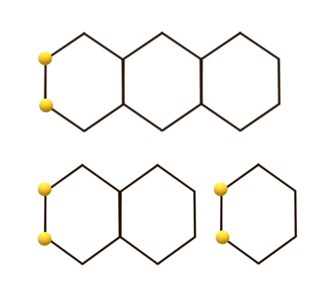
Figure 4: Three sizes of the finite hexagonal lattice with neighboring local operators.

From the simplest geometries discussed so far, we have found that while the OTOC does exhibit the decay characteristic for scrambling, finite size effects govern the dynamics. The situation becomes more interesting for hexagonal geometries.

Strip with neighboring local operators

We start with choosing the local operators to be on neighboring sites, and consider “strip” configurations with one, two, and three hexagons. For the ease of notation, we refer to lattices comprised of $n$ hexagons simply as “$n$ hex”. See Fig. 4 for an illustration. The yellow circles in each lattice indicate the support of the initially local operators in the OTOC (3).

Our results are summarized in Fig. 5. Observe that at early times, the decay of the OTOC (3) is independent of the size of the systems. Early in the evolution quantum information remains localized in the first hexagon, and only as time progresses excitations travel father into the lattice. This observation is further supported by the fact that the OTOC for 2 hex departs from the behavior of 3 hex later than the OTOC for 1 hex.

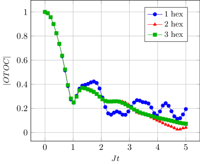
Figure 5: OTOC (3) as function of $Jt$ for a strip with neighboring local operators as illustrated in Fig. 4 for $U/J=4$ and $J=4$.

Strip with distant local operators

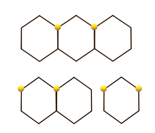
Figure 6: Three sizes of the finite hexagonal lattice with distant local operators.

The observed behavior for a second configuration is similar, while also markedly different. If the initial operators are chosen on “distant” lattice sites, as illustrated in Fig. 6, we again find the early time dynamics to be independent of the size of the system. This is depicted in Fig. 7. However, we also notice an earlier departure of the three curves, as well as a much weaker decay of the OTOC at very early times.

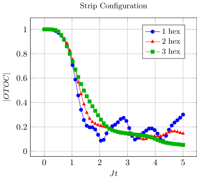
Figure 7: OTOC (3) as function of $Jt$ for a strip with distant local operators as illustrated in Fig. 6 for $U/J=4$ and $J=4$.

Bose-Hubbard flakes

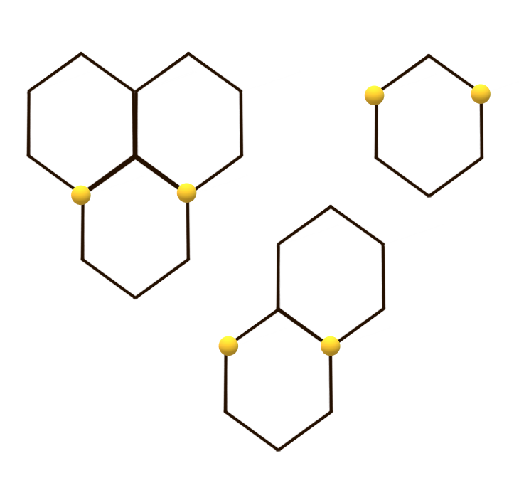
Figure 8: Three sizes of the finite hexagonal lattice, including the Bose-Hubbard flake.

As a third and final example, we solved the dynamics of a “flake” configuration with distant local operators, cf. Fig. 8. The resulting OTOC is depicted in Fig. 9. We observe qualitatively similar behavior to the strip configuration with distant local operators, cf. Fig. 7.

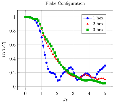
Figure 9: OTOC (3) as function of $Jt$ for the Bose-Hubbard flake for distant local operators as illustrated in Fig. 6 for $U/J=4$ and $J=4$.

III.3 Quantum chaos in the Bose-Hubbard model

As mentioned above, quantum chaotic dynamics are indicated by an exponential decay of the OTOC (3), whereas non-chaotic scrambling leads to a slower decay at early times. Thus, we fitted the initial behavior of the OTOC to a simple exponential,

$$\text{OTOC}(t)\sim\exp{\left(\lambda\,\left(t-|x|/v\right)\right)}$$ (4)

as well as to a Gaussian function,

$$\text{OTOC}(t)\sim\exp{\left(\lambda\,\left(t-|x|/v\right)^{2}\right)}\,.$$ (5)

The rationale for this particular choice will become apparent shortly. Note that $v$ is the butterfly velocity, i.e., the rate with which quasiparticle excitations travel through the lattice.

In Tab. 1 we summarize our findings for the strip with distant local operators, cf. Fig. 6. Interestingly, we find that for $1$ hex and $2$ hex, the Gaussian fit (5) describes the behavior to much higher accuracy than the exponential fit (4). However, for 3 hex the Gaussian fit predicts negative butterfly velocities, which is unphysical. Rather, the exponential fit is a much better approximation.

lattice	fit type	$\lambda$	$v$
1 hex	Gaussian	-26.310	14.754
	Exponential	-5.619	13.299
2 hex	Gaussian	-16.352	16.389
	Exponential	-16.351	8.194
3 hex	Gaussian	-3.072	-9.591
	Exponential	-3.734	12.551

Table 1: Fitting parameters for the OTOC (3) resulting from the strip with distant local operators in Fig. 7

Similar results are found for the flake configuration in Fig. 8. The fitting parameters for the OTOC depicted in Fig. 9 are summarized in Tab. 2. We find that 2 hex and 3 hex are best described with an exponential fit (4).

lattice	fit type	$\lambda$	$v$
1 hex	Gaussian	-26.310	14.754
	Exponential	-5.619	13.299
2 hex	Gaussian	-2.536	-9.848
	Exponential	-3.024	12.218
3 hex	Gaussian	-2.330	-9.481
	Exponential	-3.003	11.205

Table 2: Fitting parameters for the OTOC (3) resulting from the flake with distant local operators in Fig. 9

Our findings indicate that the dynamics in Bose-Hubbard lattices with hexagonal unit cells becomes chaotic for as little as 2 to 3 hexagons. Moreover, we observe a Gaussian to exponential transition, which strongly reminds of similar observations in decoherence theory [55].

IV Decoherence vs. Scrambling

Interestingly, such a Gaussian to exponential transition has been discussed in the literature on the decoherence factor in open quantum systems [41]. To this end, consider a composite system $\mathcal{SE}$ described by the Hamiltonian

$$H_{\mathcal{SE}}=\lambda\sigma_{z}\otimes H_{\mathcal{I}}+H_{\mathcal{E}}\,,$$ (6)

where $H_{\mathcal{I,E}}$ acts on the environment and $\sigma_{z}$ is the Pauli Z operator acting on the qubit system $\mathcal{S}$. Initializing $\mathcal{SE}$ in a product state, $\rho_{\mathcal{SE}}(0)=\rho_{\mathcal{S}}(0)\otimes\rho_{\mathcal{E}}(0)$, the decoherence function $r(t)$ can be written as

$$r(t)=\left\langle n\right|\exp{\left(iH_{\mathcal{E}}t\right)}\,\exp{\left(-i(H_{\mathcal{E}}+\lambda H_{\mathcal{P}})t\right)}\left|n\right\rangle$$ (7)

where $\left|n\right\rangle$ are the eigenstates of $H_{\mathcal{E}}$ and $H_{P}\propto H_{I}$. Note that Eq. (7) is a Loschmidt echo [56, 57, 58].

Yan and Zurek [41] then showed that Eq. (7) can be expressed as a convolution of Gaussian and exponential functions,

$$\begin{split}r(t)&\propto\exp{\left(-\tau t/2\right)}*\exp{\left(-\sigma^{2}t^{2}/2\right)}\\ &\propto\sum_{\pm}\exp{\left(\frac{\pm\tau t}{2}\right)}\,\text{Erfc}\left(\frac{\tau/2\pm\sigma^{2}t}{\sqrt{2}\sigma}\right)\end{split}$$ (8)

where $*$ denotes convolution and Erfc refers to the error function. In Ref. [41], it is shown explicitly that under rather general assumptions the overlap between the eigenstates of $H_{\mathcal{E}}$ and eigenstates of $H_{\mathcal{E}}+\lambda H_{\mathcal{P}}$ gives rise to a Lorentzian of width $\tau$, whose Fourier transform is the exponential in Eq. (8). The Gaussian contribution comes from the spectral density of the Hamiltonian containing local terms, which is assumed to be a Gaussian with standard deviation $\sigma$.

Remarkably, the same authors also showed in Ref. [55] that the Haar averaged OTOC (2) can also be written as a Loschmidt Echo. Hence, it is not far-fetched to realize that also in our present case the behavior of the OTOC (3) should be well-described by the Gausian-exponential convolution (8).

To this end, consider that a small local subsystem, i.e., a small subset of the lattices sites, is designated as system, and the remaining lattices sites as environment. Then, the local operator $A$ is chosen to live on the support of the system, and $B$ has support initially only in the environment. In this picture, it becomes immediately obvious that the OTOC (3) is identical to the decoherence function describing the loss of coherence from the “system” into the larger lattice.

Accounting for reflected quasi-particle exciations due to the finite size of the lattice, we write

$$\begin{split}\text{OTOC}(t)&=P\exp{\left(\frac{-\tau t}{2}\right)}\text{Erfc}\left(\frac{\tau/2-\sigma^{2}t}{\sqrt{2}\sigma}\right)\\ &+Q\exp{\left(\frac{\tau t}{2}\right)}\text{Erfc}\left(\frac{\tau/2+\sigma^{2}t}{\sqrt{2}\sigma}\right)\end{split}$$ (9)

where $P$ and $Q$ are free parameters. Using Eq. (9) we fitted our earlier results again, and the results are summarized in Tabs. 3 and 4.

lattice	$\tau$	$\sigma$	$\tau/\sigma$
1 hex	1.822	0.122	14.934
2 hex	1.707	0.163	10.472
3 hex	0.751	1.138	0.660

Table 3: Fitting parameters for the OTOC (3) as convolution function (9) resulting from the strip with distant local operators in Fig. 7.

lattice	$\tau$	$\sigma$	$\tau/\sigma$
1 hex	1.822	0.122	14.934
2 hex	0.495	0.875	0.566
3 hex	0.667	0.954	0.699

Table 4: Fitting parameters for the OTOC (3) as convolution function (9) resulting from the flake with distant local operators in Fig. 9

Note that when $\tau\gg\sigma$, the convolution function Eq. (8) reduces to a Gaussian whereas when $\tau\ll\sigma$, it reduces to an exponential. We immediately observe that (i) the convolution is a much better description of the OTOC, and (ii) that the more sophisticated fit is consistent with our above results.

More importantly, we conclude that for two-dimensional Bose-Hubbard lattices, the behavior of the OTOC is remarkably well-described by a decoherence model. This is consistent with earlier findings that highlight the close relationship of information scrambling and decoherence [5].

V Concluding remarks

In this paper, we have studied the notion of information scrambling in two-dimensional lattices described by the Bose-Hubbard model. We have found that for as little as 2 hexagons the OTOC shows the characteristic exponential decay indicating quantum chaotic behavior. However, we have also found that the scrambling dynamics is highly sensitive to the choice of local operators and lattice configuration. In particular, for “flake” configurations the OTOC decays more akin to a decoherence functions as described by a Gaussian-exponential convolution, rather than exhibiting a chaotic, exponential decay.

Appendix A Scrambling in 1D

For completeness and to verify our numerical approach, we also solved for the dynamics of the one-dimensional Bose-Hubbard model. As for the two-dimensional case, we computed the OTOC (3) and also other quantifiers of scrambling.

Mutual Information

In Ref. [59] it was shown that the mutual information is a thermodynamically well-motivated quantifier of scrambling. For two subsystems $A$ and, $B$ the bipartite mutual information between $A$ and $B$ is given by

$$I(A:B)=S_{A}+S_{B}-S_{AB}$$ (10)

where $S_{X}=-\mathrm{tr}\left\{\rho_{X}\ln{\rho_{X}}\right\}$ is the Von-Neumann entropy of the corresponding subsystem $X$.

In Ref. [59], it was shown that the change in Haar-averaged OTOC is upper bounded by the change in bipartite mutual information:

$$\Delta\langle\text{OTOC}(t)\rangle_{Haar}\leq\Delta I(A:B)(t)$$ (11)

where $\Delta\langle\text{OTOC}(t)\rangle_{Haar}=1-\langle\text{OTOC}(t)\rangle_{Haar}$ is a monotonically growing function. This means that $\Delta I(A:B)$ also has to be growing in time.

Tripartite Mutual Information

Another such information-theoretic quantity that does not depend on the choice of operators is Tripartite Mutual Information (TMI). The Tripartite Mutual Information(TMI) between the three subsystems $A$ and $B$ and $C$ reads

$$I_{3}(A:B:C)=I(A:B)+I(A:C)-I(A:BC)$$ (12)

Information is said to be scrambled for systems comprised of $B\otimes C$ if TMI becomes negative [24, 60, 61, 62]. This means that the information about $A$ in $BC$ combined has to be greater than the total information about $A$ that $B$ and $C$ have separately.

Numerical results

Various measures of scrambling for one hexagonal lattice with 6 sites, 6 bosons and local operators defined over any two nearest neighbor sites on the lattice are shown in Fig. 10. We find that the Bose Hubbard model shows information scrambling only when $U\gg J$.

The OTOC shows a rapid decay followed by small oscillations. Mutual Information, over equal bi-partitions of the system, rises rapidly and oscillates about a steady value thereafter. We find that the OTOC for a specific choice of operators (not averaged over) also obeys (11). The initial state for TMI is $\left|\psi\right\rangle=(\left|0\right\rangle_{A}\left|1\right\rangle_{B}+\left|1\right\rangle_{A}\left|0\right\rangle_{B})\left|1,1\right\rangle_{C}\left|1,1,1\right\rangle_{D}$ where $BCD$ evolves via the Bose-Hubbard Hamiltonian and $A$ remains stationary. The TMI becomes negative and fluctuates about a steady negative value afterward. Therefore, we find that all three quantities indicate the scrambling of quantum information in the Bose Hubbard Model, which confirms the validity of our approach.

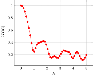
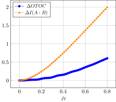
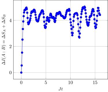
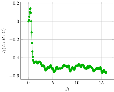
Figure 10: Information Scrambling in the one-dimensional Bose Hubbard model. The scrambling of this model is consistently captured by the bipartite, tripartite mutual information, and the OTOC for $U/J=4$ and $J=4$

References

- scr [2022] The history of scrambled eggs (2022).
- qua [2019] Happy easter: looking for quantum eggs (2019).
- qua [2021] Quantum egg (2021).
- Touil and Deffner [2024] A. Touil and S. Deffner, Information scrambling – a quantum thermodynamic perspective, arXiv preprint arXiv:2401.05305 (2024).
- Touil and Deffner [2021] A. Touil and S. Deffner, Information scrambling versus decoherence—two competing sinks for entropy, PRX Quantum 2, 010306 (2021).
- Roberts and Swingle [2016a] D. A. Roberts and B. Swingle, Lieb-robinson bound and the butterfly effect in quantum field theories, Phys. Rev. Lett. 117, 091602 (2016a).
- Anand and Zanardi [2022] N. Anand and P. Zanardi, BROTOCs and Quantum Information Scrambling at Finite Temperature, Quantum 6, 746 (2022).
- Yuan et al. [2022] D. Yuan, S.-Y. Zhang, Y. Wang, L.-M. Duan, and D.-L. Deng, Quantum information scrambling in quantum many-body scarred systems, Phys. Rev. Res. 4, 023095 (2022).
- Hayden and Preskill [2007] P. Hayden and J. Preskill, Black holes as mirrors: quantum information in random subsystems, JHEP 2007 (09), 120.
- Blok et al. [2021] M. S. Blok, V. V. Ramasesh, T. Schuster, K. O’Brien, J. M. Kreikebaum, D. Dahlen, A. Morvan, B. Yoshida, N. Y. Yao, and I. Siddiqi, Quantum information scrambling on a superconducting qutrit processor, Phys. Rev. X 11, 021010 (2021).
- Huang et al. [2017] Y. Huang, Y.-L. Zhang, and X. Chen, Out-of-time-ordered correlators in many-body localized systems, Ann. Phys. 529, 1600318 (2017).
- Yunger Halpern [2017] N. Yunger Halpern, Jarzynski-like equality for the out-of-time-ordered correlator, Phys. Rev. A 95, 012120 (2017).
- Swingle [2018] B. Swingle, Unscrambling the physics of out-of-time-order correlators, Nat. Phys. 14, 988 (2018).
- Hashimoto et al. [2017] K. Hashimoto, K. Murata, and R. Yoshii, Out-of-time-order correlators in quantum mechanics, JHEP 2017 (10), 138.
- Li et al. [2023] H. Li, E. Halperin, R. R. W. Wang, and J. L. Bohn, Out-of-time-order correlator for the van der waals potential, Phys. Rev. A 107, 032818 (2023).
- Roberts et al. [2015] D. A. Roberts, D. Stanford, and L. Susskind, Localized shocks, JHEP 2015 (3), 51.
- Roberts and Stanford [2015] D. A. Roberts and D. Stanford, Diagnosing chaos using four-point functions in two-dimensional conformal field theory, Phys. Rev. Lett. 115, 131603 (2015).
- Fan et al. [2017] R. Fan, P. Zhang, H. Shen, and H. Zhai, Out-of-time-order correlation for many-body localization, Science Bulletin 62, 707 (2017).
- Swingle et al. [2016] B. Swingle, G. Bentsen, M. Schleier-Smith, and P. Hayden, Measuring the scrambling of quantum information, Phys. Rev. A 94, 040302 (2016).
- Cotler et al. [2018] J. S. Cotler, D. Ding, and G. R. Penington, Out-of-time-order operators and the butterfly effect, Ann. Phys. 396, 318 (2018).
- Maldacena et al. [2016] J. Maldacena, S. H. Shenker, and D. Stanford, A bound on chaos, JHEP 2016 (8), 106.
- Xu et al. [2020] T. Xu, T. Scaffidi, and X. Cao, Does scrambling equal chaos?, Phys. Rev. Lett. 124, 140602 (2020).
- Maldacena and Stanford [2016a] J. Maldacena and D. Stanford, Remarks on the sachdev-ye-kitaev model, Phys. Rev. D 94, 106002 (2016a).
- Iyoda and Sagawa [2018] E. Iyoda and T. Sagawa, Scrambling of quantum information in quantum many-body systems, Phys. Rev. A 97, 042330 (2018).
- Sahu et al. [2019] S. Sahu, S. Xu, and B. Swingle, Scrambling dynamics across a thermalization-localization quantum phase transition, Phys. Rev. Lett. 123, 165902 (2019).
- Sahu and Swingle [2020] S. Sahu and B. Swingle, Information scrambling at finite temperature in local quantum systems, Phys. Rev. B 102, 184303 (2020).
- Sachdev and Ye [1993] S. Sachdev and J. Ye, Gapless spin-fluid ground state in a random quantum heisenberg magnet, Phys. Rev. Lett. 70, 3339 (1993).
- Maldacena and Stanford [2016b] J. Maldacena and D. Stanford, Remarks on the sachdev-ye-kitaev model, Phys. Rev. D 94, 106002 (2016b).
- Rosenhaus [2019] V. Rosenhaus, An introduction to the syk model, J. Phys. A: Math. Theoret. 52, 323001 (2019).
- Plugge et al. [2020] S. Plugge, E. Lantagne-Hurtubise, and M. Franz, Revival dynamics in a traversable wormhole, Phys. Rev. Lett. 124, 221601 (2020).
- Kolovsky [2016] A. R. Kolovsky, Bose–hubbard hamiltonian: Quantum chaos approach, Int. J. Mod. Phys. B 30, 1630009 (2016).
- Shen et al. [2017] H. Shen, P. Zhang, R. Fan, and H. Zhai, Out-of-time-order correlation at a quantum phase transition, Phys. Rev. B 96, 054503 (2017).
- Freericks and Monien [1994] J. K. Freericks and H. Monien, Phase diagram of the bose-hubbard model, EPL (Europhysics Letters) 26, 545 (1994).
- Gardas et al. [2017] B. Gardas, J. Dziarmaga, and W. H. Zurek, Dynamics of the quantum phase transition in the one-dimensional bose-hubbard model: Excitations and correlations induced by a quench, Phys. Rev. B 95, 104306 (2017).
- Dziarmaga and Mazur [2023] J. Dziarmaga and J. M. Mazur, Tensor network simulation of the quantum kibble-zurek quench from the mott to the superfluid phase in the two-dimensional bose-hubbard model, Phys. Rev. B 107, 144510 (2023).
- Wang and Jiang [2016] B. Wang and Y. Jiang, Bogoliubov approach to superfluid-bose glass phase transition of a disordered bose-hubbard model in weakly interacting regime, The European Physical Journal D 70, 10.1140/epjd/e2016-70459-y (2016).
- Kollath et al. [2007] C. Kollath, A. M. Läuchli, and E. Altman, Quench dynamics and nonequilibrium phase diagram of the bose-hubbard model, Phys. Rev. Lett. 98, 180601 (2007).
- Nakerst and Haque [2023] G. Nakerst and M. Haque, Chaos in the three-site bose-hubbard model: Classical versus quantum, Phys. Rev. E 107, 024210 (2023).
- T.O. Wehling and Balatsky [2014] A. B.-S. T.O. Wehling and A. Balatsky, Dirac materials, Ad. Phys. 63, 1 (2014).
- González Alonso et al. [2019] J. R. González Alonso, N. Yunger Halpern, and J. Dressel, Out-of-time-ordered-correlator quasiprobabilities robustly witness scrambling, Phys. Rev. Lett. 122, 040404 (2019).
- Yan and Zurek [2022] B. Yan and W. H. Zurek, Decoherence factor as a convolution: an interplay between a gaussian and an exponential coherence loss, New J. Phys. 24, 113029 (2022).
- Arovas et al. [2022] D. P. Arovas, E. Berg, S. A. Kivelson, and S. Raghu, The hubbard model, Ann. Rev. Cond. Matt. Phys. 13, 239 (2022).
- Dutta et al. [2015] O. Dutta, M. Gajda, P. Hauke, M. Lewenstein, D.-S. Lühmann, B. A. Malomed, T. Sowiński, and J. Zakrzewski, Non-standard hubbard models in optical lattices: a review, Rep. Prog. Phys. 78, 066001 (2015).
- Greiner et al. [2002] M. Greiner, O. Mandel, T. Esslinger, T. W. Hänsch, and I. Bloch, Quantum phase transition from a superfluid to a mott insulator in a gas of ultracold atoms, Nature 415, 39 (2002).
- Dziarmaga and Zurek [2014] J. Dziarmaga and W. H. Zurek, Quench in the 1d bose-hubbard model: Topological defects and excitations from the kosterlitz-thouless phase transition dynamics, Scientific Reports 4, 5950 (2014).
- Shimizu et al. [2018] K. Shimizu, Y. Kuno, T. Hirano, and I. Ichinose, Dynamics of a quantum phase transition in the bose-hubbard model: Kibble-zurek mechanism and beyond, Phys. Rev. A 97, 033626 (2018).
- Weiss et al. [2018] W. Weiss, M. Gerster, D. Jaschke, P. Silvi, and S. Montangero, Kibble-zurek scaling of the one-dimensional bose-hubbard model at finite temperatures, Phys. Rev. A 98, 063601 (2018).
- Goldstein et al. [2002] H. Goldstein, C. Poole, and J. Safko, Classical mechanics (American Association of Physics Teachers, 2002).
- Shenker and Stanford [2014] S. H. Shenker and D. Stanford, Black holes and the butterfly effect, JHEP 2014 (3), 1.
- Gong et al. [2023] Z. Gong, T. Guaita, and J. I. Cirac, Long-range free fermions: Lieb-robinson bound, clustering properties, and topological phases, Phys. Rev. Lett. 130, 070401 (2023).
- Nachtergaele et al. [2009] B. Nachtergaele, H. Raz, B. Schlein, and R. Sims, Lieb-robinson bounds for harmonic and anharmonic lattice systems, Comm. Math. Phys. 286, 1073 (2009).
- Hastings [2010] M. B. Hastings, Locality in quantum systems (2010), arXiv:1008.5137 [math-ph] .
- Roberts and Swingle [2016b] D. A. Roberts and B. Swingle, Lieb-robinson bound and the butterfly effect in quantum field theories, Physical review letters 117, 091602 (2016b).
- Ford [2015] W. Ford, Chapter 21 - krylov subspace methods, in Numerical Linear Algebra with Applications, edited by W. Ford (Academic Press, Boston, 2015) pp. 491–532.
- Yan et al. [2020] B. Yan, L. Cincio, and W. H. Zurek, Information scrambling and loschmidt echo, Phys. Rev. Lett. 124, 160603 (2020).
- Cucchietti [2004] F. M. Cucchietti, The loschmidt echo in classically chaotic systems: Quantum chaos, irreversibility and decoherence (2004), arXiv:quant-ph/0410121 [quant-ph] .
- Gorin et al. [2006] T. Gorin, T. Prosen, T. H. Seligman, and M. Žnidarič, Dynamics of loschmidt echoes and fidelity decay, Phys. Rep. 435, 33 (2006).
- Ares and Wisniacki [2009] N. Ares and D. A. Wisniacki, Loschmidt echo and the local density of states, Phys. Rev. E 80, 046216 (2009).
- Touil and Deffner [2020] A. Touil and S. Deffner, Quantum scrambling and the growth of mutual information, Quantum Science and Technology 5, 035005 (2020).
- Seshadri et al. [2018] A. Seshadri, V. Madhok, and A. Lakshminarayan, Tripartite mutual information, entanglement, and scrambling in permutation symmetric systems with an application to quantum chaos, Phys. Rev. E 98, 052205 (2018).
- Hosur et al. [2016] P. Hosur, X.-L. Qi, D. A. Roberts, and B. Yoshida, Chaos in quantum channels, JHEP 2016 (2), 4.
- Han et al. [2022] L.-P. Han, J. Zou, H. Li, and B. Shao, Quantum information scrambling in non-markovian open quantum system, Entropy 24, 10.3390/e24111532 (2022).